Abstract
(1) Background: Diabetes is a common chronic disease and a leading cause of death. Early diagnosis gives patients with diabetes the opportunity to improve their dietary habits and lifestyle and manage the disease successfully. Several studies have explored the use of machine learning (ML) techniques to predict and diagnose this disease. In this study, we conducted experiments to predict diabetes in Pima Indian females with particular ML classifiers. (2) Method: A Pima Indian diabetes dataset (PIDD) with 768 female patients was considered for this study. Different data mining operations were performed to a conduct comparative analysis of four different ML classifiers: Naïve Bayes (NB), J48, Logistic Regression (LR), and Random Forest (RF). These models were analyzed by different cross-validation (K = 5, 10, 15, and 20) values, and the performance measurements of accuracy, precision, F-score, recall, and AUC were calculated for each model. (3) Results: LR was found to have the highest accuracy (0.77) for all ‘k’ values. When k = 5, the accuracy of J48, NB, and RF was found to be 0.71, 0.76, and 0.75. For k = 10, the accuracy of J48, NB, and RF was found to be 0.73, 0.76, 0.74, while for k = 15, 20, the accuracy of NB was found to be 0.76. The accuracy of J48 and RF was found to be 0.76 when k = 15, and 0.75 when k = 20. Other parameters, such as precision, f-score, recall, and AUC, were also considered in evaluations to rank the algorithms. (4) Conclusion: The present study on PIDD sought to identify an optimized ML model, using with cross-validation methods. The AUC of LR was 0.83, RF 0.82, and NB 0.81). These three were ranked as the best models for predicting whether a patient is diabetic or not.
1. Introduction
Diabetes is a common chronic disease occurring when the pancreas does not produce enough insulin (Type 1 diabetes) or when the patient’s body does not effectively utilize the insulin (Type 2 diabetes). Hyperglycemia or raised blood sugar is the common consequence of uncontrolled diabetes. Over time, diabetes can cause severe damage to nerves and blood vessels [1]. Advanced diabetes is complicated by coronary illness, visual impairment, and kidney failure [1,2]. Early detection of the disease can give patients the opportunity to make the necessary lifestyle changes and therefore can improve their life expectancy [3].
Machine learning (ML), is an application of artificial intelligence (AI) that enables computers to self-learn and perform statistical analysis without human interaction [4]. ML algorithms and models are extensively used and have been found reliable for a variety of applications. Researchers have been adopting ML in medicine, especially for diagnosis, disease prediction [5], drug discovery, and clinical trials [6].
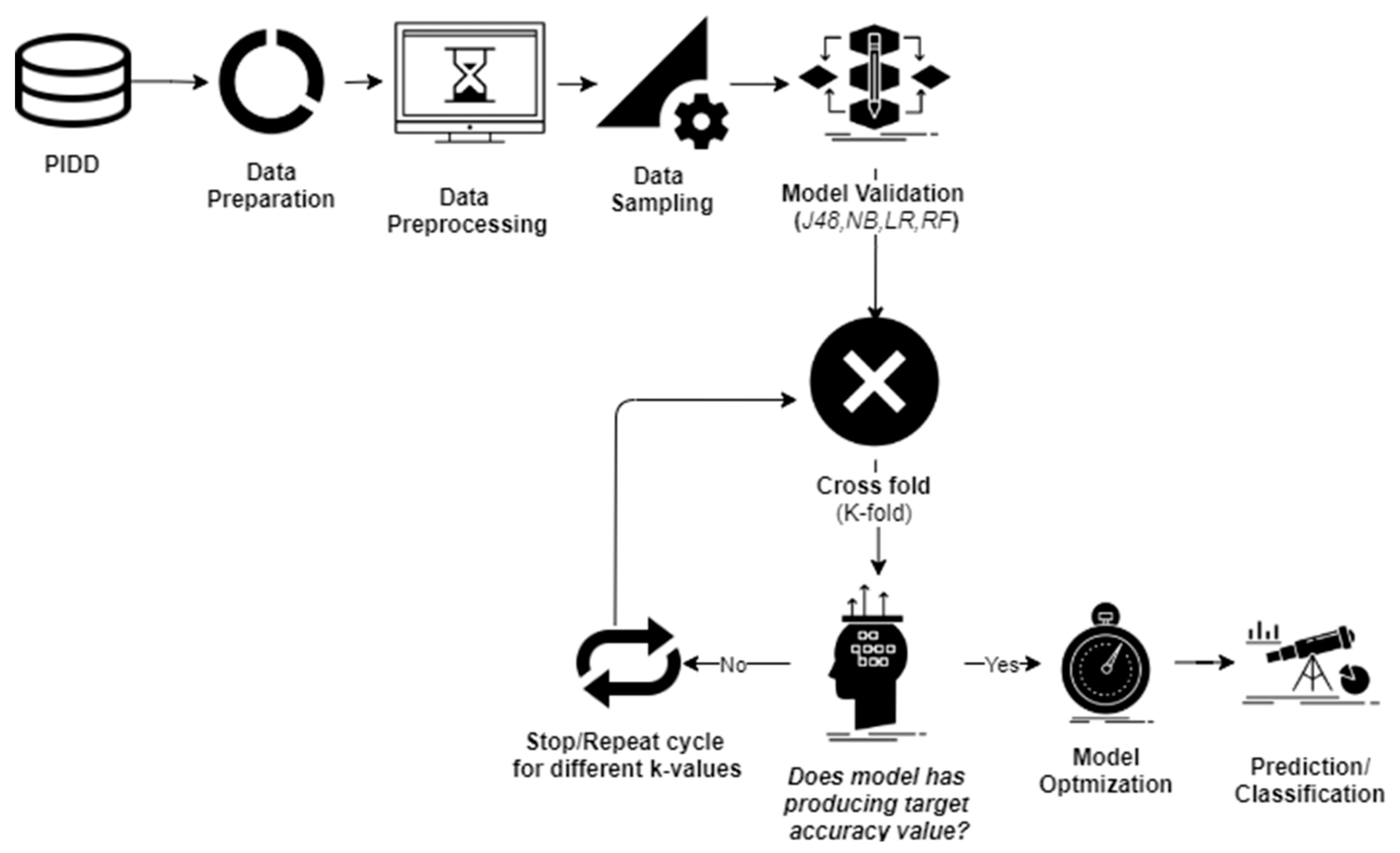
The machine learning process starts with structured or unstructured data from different sources. The next step is data preparation or data preprocessing, which involves data selection through a data mining method in which original or raw data is converted into an understandable format [7]. Once the data is ready, the model tests different trained data-sets to calculate accuracy or perform statistical algorithms; this is known as model validation [8]. Model optimization or model improvement is done by hyperparameter tuning for final validation to perform prediction, and classification (Figure 1).

Figure 1.
The primary mechanisms of machine learning.
In healthcare systems, large amounts of patient data and medical knowledge are stored in databases, and new tools and technologies for data analysis and classification are needed to exploit this information. Currently, ML algorithms are used for the automatic analysis of high dimensional medical data. Dementia forecasting [9], cancer tumor identification [10], diabetes predictions [11], and radiotherapy [12] are some examples of ML in medicine.
According to World Health Organization (WHO) reports, there are 425 million people in the world with diabetes [13]. Extensive studies on the diagnosis and early prediction of diabetes have shown that the risk factors associated with Type 2 diabetes include family history, hypertension, unhealthy diet, lack of physical activities, and being overweight. Females have a higher tendency to become diabetic (especially during pregnancy), due to low insulin absorption, high cholesterol levels, or a rise in blood pressure [13,14]. Studies have shown that cost-effective and efficient techniques for diagnosing diabetes could be developed by employing computer skills and data mining algorithms.
Several studies conduct prediction analysis using data-mining algorithms to diagnose diabetes. For example, in [15], researchers utilized support vector machines (SVM) for the diagnosis of diabetes mellitus and achieved a prediction accuracy of about 94%. Another work has used J48 decision trees, RF, and neural networks, and has found that RF provides the highest accuracy (80.4%) in diabetic patient classification [16]. Another paper proposed a model to forecast the likelihood of diabetes. This study concluded that Naïve Bayes (NB) had 76.3% accuracy, higher than J48 and SVM [17]. An accuracy analysis conducted on different ways of data preprocessing, and parameter modification was done to improve model precision [18]. The above results revealed that deep neural networks (DNN) with cross-validation (K = 10) generated 77.86% accuracy in diabetes identification.
In this study, we developed a classification model for Type 2 diabetes in Pima Indian females. Four classification ML algorithms to detect diabetes in female patients were used: J48 decision trees, NB, RF, and Logistic Regression (LR). Cross-validation (CV) techniques were employed to train the different ML models for varying test data-sets. The ranking of each algorithm was decided based on the performance parameters of accuracy, precision, recall, and F-scores.
2. Methods and Materials
A Pima Indian diabetes dataset (PIDD) with 768 female patients was considered. This dataset, owned by the National Institute of Diabetes and Digestive and Kidney Diseases (NIDDK), contained a tested positive (class variable: 1) and a tested negative (class variable: 0) with eight various risk factors (Table 1).

Table 1.
Statistical report of the Pima Indian diabetes dataset (PIDD).
Data investigation was undertaken using WEKA 3.8 [19], which is an open-source tool that can help to perform various data-mining operations. At first, PIDD was exposed to data preprocessing steps to control the unbalanced data-sets (Figure 2).

Figure 2.
Applied methodology.
2.1. Data Sampling
Two data sampling techniques were used to convert imbalanced datasets into balanced datasets: oversampling (on the minority class instances), and under-sampling (on the majority class instances). Different forms of the PIDD dataset with statistical values of each attribute are presented in Table 2.

Table 2.
Statistics of original and different trained sets (where SD: standard deviation, BMI: Body Mass Index).
2.2. Cross-Validation
Cross-validation (CV) is a model training method that can assess prediction accuracy [20]. The biggest challenge in ML is validating the model with trained data. To ensure the adopted model is producing the noise-free model patterns [21], data scientists use CV techniques. Compared with other methods, the CV technique offers the most ease in estimating low bias models, and therefore is one of the most popular techniques in ML algorithms.
In this study, four ML classifiers were employed to conduct different cross-validations. The k-fold CV technique was used to perform model validation. The PIDD was split into ‘k’ folds to conduct training with test data, and the remaining ‘k-1’ folds were combined to form trained data. Original data were randomly separated into ‘k’ folds (k1,k2…,ki), and the model testing was performed by ‘k’ times. For example, in the first iteration, if subset (k1) served as test data, then the remaining subsets (k2,……,ki) were combined to conduct model training, and this process was repeated for the rest of the ‘k’ values. Many studies reported that in order to avoid issues associated with imbalanced data-sets, the optimal value for ‘k’ should be 5 or 10. With the highest (k) values, the difference in trained and sampled data-sets tended to acquire low values. In the present study, model validation was conducted with k = 5, 10, 15, and 20.
2.3. Naïve Bayes (NB)
Naïve Bayes (NB) is a probability-based ML method that can be used as a classification technique. Based on feature extraction, NB produces the probability for target groups in classification [22]. This algorithm quickly and easily predicts the test data and produces better performance values in multi-class predictions. Compared with numerical inputs, NB predicts correctly categorical input values. The Bayes theorem is represented in Equation (1) below
The probability of ‘c’ is happening, given that ‘X’ occurrence.
Here, P (c/X) = target class’s posterior probability,
P (X/c) = predictor class’s probability,
P(c) = class ‘c’s probability is true,
P(X) = predictor’s prior probability.
2.4. Logistic Regression (LR)
LR is a classification algorithm used to allocate observations into discrete set of classes. It is classified into the binary, multi, and normal level types. LR does not indicate a relationship between non-continuous attributes, but allows the prediction of the discrete variables [23]. It is very easy to implement and quite efficient for training the model.
Logistic regression is mathematically written as a multiple linear regression function Equation (2) by
The following example represents a simple logistic binary function. As discussed, two target diabetic groups (tested positive-‘1’ or tested negative-‘0’) were tested
Hypothesis W = AX + B
H (x) = sig (W)
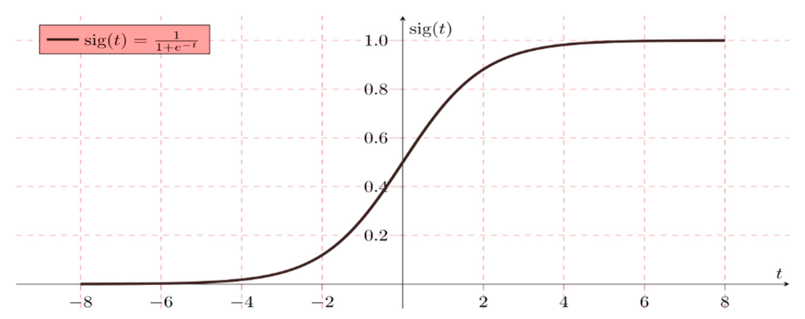
If ‘W’ reaches positive infinity, then the prediction is positive, and if ‘W’ reaches to negative infinity, then the prediction is negative (Figure 3).
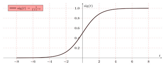
Figure 3.
Simple binary logistic regression representation (where sig (t) sigmoid activation function).
2.5. Random Forest (RF)
When feature selection methods are used, the RF algorithm is quick to learn to produce the highest classification accuracy on large databases, because of the tree-based systems used. Generally, these trees are nicely positioned for improving the virtue of the tree node known as the Gini impurity [24]. In RF, feature extraction is conducted from the test data. Thereafter, test features are validated by the randomly generated decision trees (Figure 4). In the example of PIDD, if the model was generated 50 random trees, every tree could predict two different outcomes for the same test group. If 30 trees were predicted (tested positive) and 20 trees were predicted (tested negative), then the RF algorithm returns ‘tested positive’ as the predicted target.

Figure 4.
Random forest (RF) procedure flow chart representation.
2.6. J48 (Decision Tree Algorithm)
J48 or decision tree algorithm allows to calculate the feature behavior of different test groups. With J48, it is easy to understand the explanatory distribution of instances. This can help in identifying missing attributes and therefore works as a precision tool in case of over fitting was occurred [25]. The major challenge associated with the decision trees is the identification of the root node attribute. This attribute selection can be done in two methods: information gain Equation (5) and Gini Index Equation (6).
Here, X: Set of instances, A: attribute, XX: a subset of X with A = X, and value (A): set of total possible values of A.
Gini index (GI) is a parameter that helps to calculate how often randomly selected instances could be incorrectly classified.
2.7. Performance Measures
Model performance was decided on the basis of accuracy, precision, recall, and F-scores. The performance measures with formulation and definitions are provided in Table 3.

Table 3.
Definition and formulation of accuracy measures (where TP: true positive; TN: true negative; FP: false positive; FN: false negative).
3. Results
Due to the issues raised with the model over fitting, exclusion of over-sampling and under-sampling PIDD data-sets were done during experiments.
3.1. Pruned Decision Tree
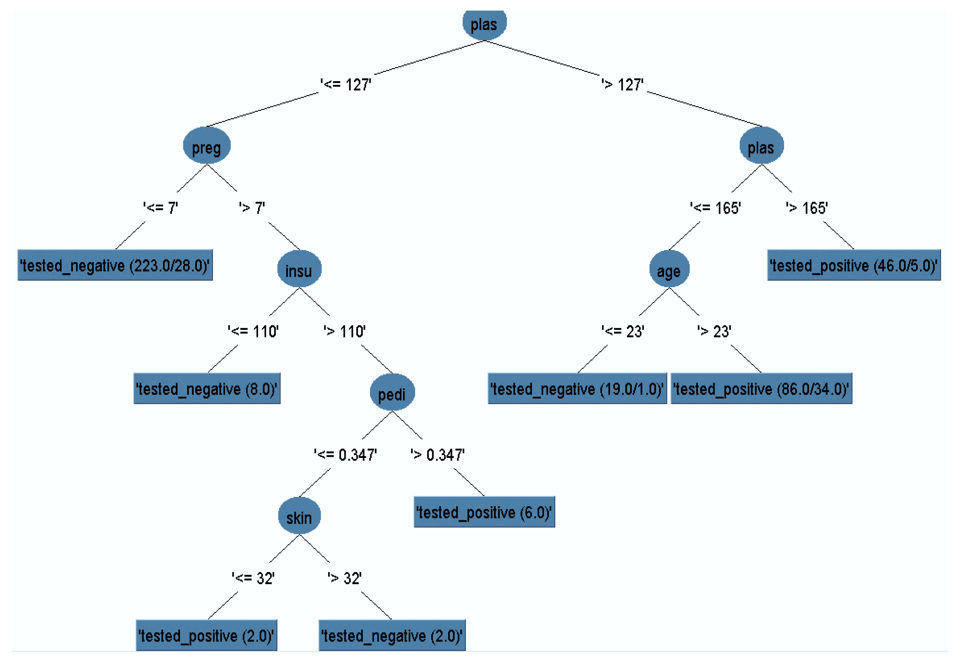
The J48 model classifier was exposed with the remained dataset (after removal of missing instances) to generate a pruned decision tree. The output pruned decision tree with plasma value as a central node is represented in Figure 5. It is obvious that plasma glucose concentration has the highest information gain, which could be considered as the highest risk factor for diabetes. Other risk factors such as multiple pregnancies, release of high levels of insulin, and lineage function also increased the chances of having diabetes. Generally, pregnant women who do not take much physical exercise have higher chances of gaining weight, which in turn increases the likelihood of having Type 2 diabetes.

Figure 5.
Pruned decision tree.
3.2. Confusion Matrix
The confusion matrix was used to describe the performance of various model classifiers [26]. The simulation was conducted with the four ML classifiers to analyze the accuracy of the prediction of the test class (Table 4).

Table 4.
Confusion matrix of different classifier models.
3.3. Model Classification
We conducted the experiments with four ML classifiers to diagnose whether the patient was diabetic or non-diabetic. Table 5 shows the hyper parameters of four classifiers trained to classify diabetes of female patients. Performance measures validated all the models, exposed to different cross-validations to conduct model optimization techniques. The performance of four models chosen was depending on accuracy, recall, precision, AUC (area under the curve), and F-scores as shown in Table 6.

Table 5.
Hyperparameters of different classifiers (here C: pruning confidence and ‘R’–R squared value).

Table 6.
Performance measures of different model classifiers (where k = 5, 10, 15&20).
4. Discussion
Diabetes diagnosis at an early stage will give patients the opportunity to treat the disease and change their lifestyle in time to achieve positive results. In the present study, we propose an optimized machine learning algorithm for classifying and diagnosing Pima diabetic patients.
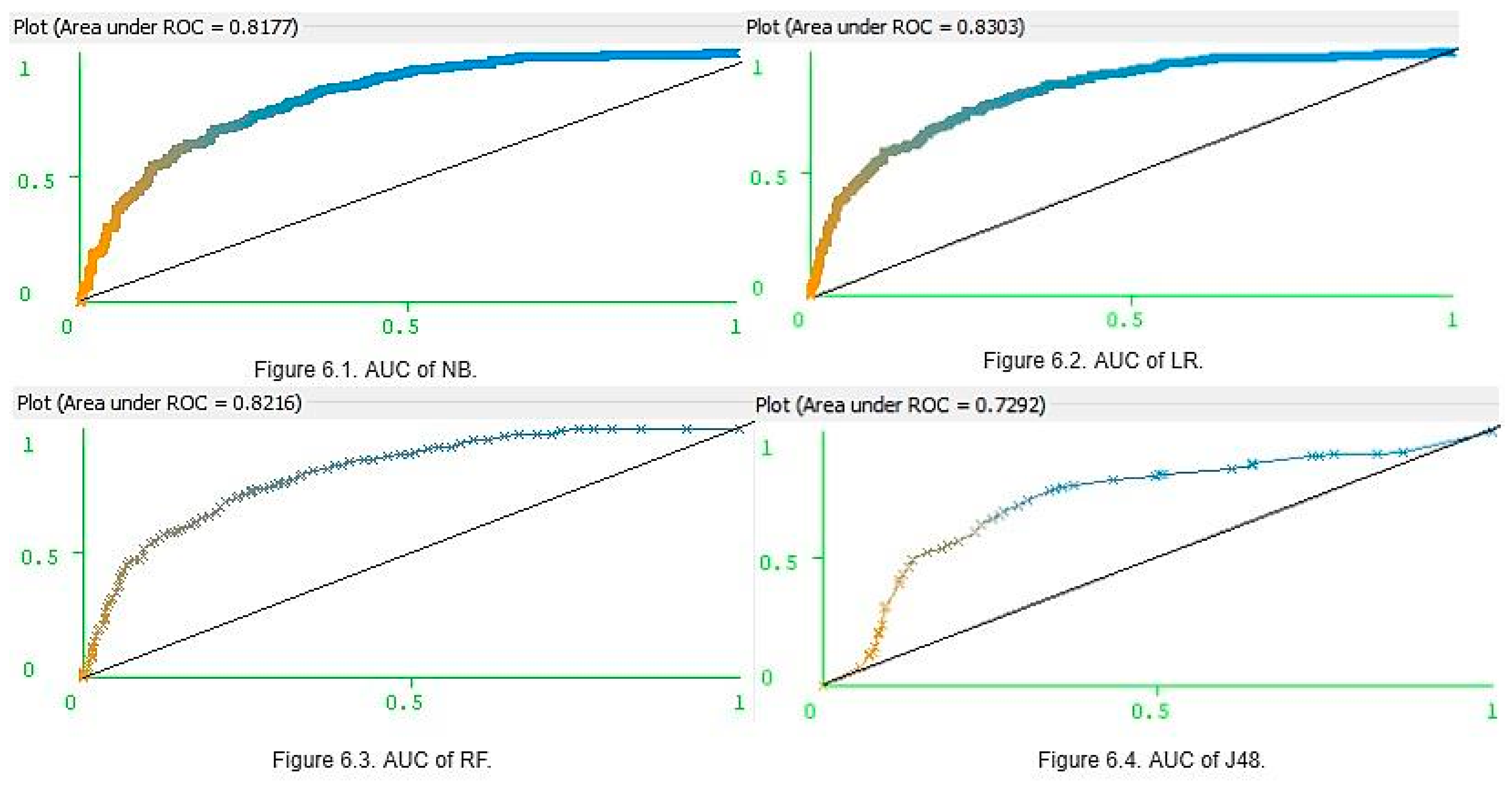
The majority of the results produced almost identical accuracy values. Hence, for assigning rankings for each model, Receiver Optimistic Curve (ROC) rates were used. ROC is a visualizing tool of the performance of the binary classifier. It is generated by plotting a false positive rate on the X-axis against the true positive rate on the Y-axis in order to decide the correct threshold value [27]. The AUC is the rate of accurate model classification and typically ranges between 0.5 and 1.0. If AUC is near to 1, the model performs correct classification of instances, and results in good optimization [28]. Four different machine learning algorithms were employed for various k values to predict whether a patient was diabetic or non-diabetic. Dataset was split into ‘k’ subsets to perform training and testing (in ‘k’ times). All preliminary analysis was carried out with the help of WEKA studio.
To avoid over fitting and under fitting issues, tenfold cross-validation was considered. The highest accuracy was achieved when the trained data had been exposed to k = 10. From Table 6, it was found that the LR model with the highest accuracy of 0.77, and NB, J48, and RF had an accuracy of 0.76, 0.73, and 0.74 respectively. In addition, recall (sensitivity) defines the rate of correctly predicted diabetic patients. For LR, it was found to be 0.77, and for RF, J48, and NB, it was recorded as 0.74, 0.73, and 0.76. The precision of NB was 0.75 that of J48 was 0.73, RF was 0.74, and LR was 0.76. F scores of J48, NB, RF, and LR were 0.73, 0.76, 0.74, and 0.76 respectively. In addition, we calculated the AUC to measure the performance of the four models. The AUC of J48, NB, RF, and LR was generated as 0.75, 0.81, 0.81, and 0.83.
These results clearly show that the four classifiers had similar prediction accuracy with small differences and margins of error. However, LR was the most accurate and J48 was the least accurate. Ultimately, LR, NB, and RF were deemed to be the three best models for predicting whether a patient is diabetic or not. Furthermore, for K = (5, 10, and 20), the NB parameters for accuracy, precision, recall, and f-scores were higher than those of RF. However, for K = 15, the RF precision and F-scores were higher than those of NB. Accuracy was not only the parameter, which can be used in assessing model optimization. The main limitation in using accuracy as the key performance metric is that it does not work well in datasets. This can generate class imbalances. The PIDD (Table 1) contains 500 women who tested negative for diabetes, and 268 women who tested positive for diabetes, and thus the imbalance ratio is 1.87. Hence, along with accuracy, it is also important to consider the AUC values (Figure 6). The AUC values of NB (Figure 6.1) and LR (Figure 6.2) were 0.81 and 0.83, respectively, and for RF (Figure 6.3), it was 0.82 and 0.81. However, J48 produced a lower AUC value (0.72) than others (Figure 6.4). When each classifier is ranked according to performance values, once seems that an optimized model is LR > RF > NB > J48.
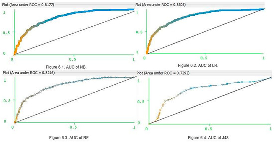
Figure 6.
Area under the curve (AUC) of four different classifiers.
5. Conclusions
Diabetes is one of the most critical chronic diseases today, and early diagnosis can help greatly in improving a patient’s chances of managing it well. The latest developments in machine intelligence can be exploited to improve our understanding of the factors causing the onset of this disease. We developed four binary classifier models: NB, J48, LR, and RF, and each model was analyzed using different CV methods (subject to different ‘k’ values). Performance assessment was conducted with the parameters of accuracy, precision, recall, F-scores, and AUC. Preliminary outcomes suggested that all models investigated achieved good results, with the LR model showing the greatest accuracy (0.77), and the J48 the relatively low accuracy compared to the others. Ranking conducted by considering not only accuracy but also other parameters, and indicated that LR, NB, RF are the three best models for predicting whether a patient is diabetic or not.
The main limitation of this stdy is that only the conventional ML classifiers were considered. Since the results provide an improvement on existing methods for predicting diabetes, it would be worthwhile in future studies to explore these models in unsupervised machine learning and deep learning techniques as well.
Author Contributions
We certify that the manuscript is not under review by any other journal. All authors have read and validated the final copy of this manuscript. G.B.: Design and perform the experiments. Analyze the methods, results, and wrote the manuscript. C.N. & G.G.S.: Contribute to the literature review, S.K.T. & F.A.: Conclusion and final manuscript revision.
Funding
This research received no external funding.
Acknowledgments
This study was supported by an institutional grant of Camerino University. Gopi B, Getugamo S, Nalini Ch Ph.D. bursaries were supported by the University of Camerino. The English language editing by Sheilla Beatty is gratefully acknowledged.
Conflicts of Interest
The authors declare no conflict of interest.
References
- Seshasai, S.R.K.; Kaptoge, S.; Thompson, A.; Di Angelantonio, E.; Gao, P.; Sarwar, N.; Whincup, P.H.; Mukamal, K.J.; Gillum, R.F.; Holme, I.; et al. Diabetes mellitus, fasting glucose, and risk of cause-specific death. N. Engl. J. Med. 2011, 364, 829–841. [Google Scholar]
- Chatterjee, S.; Khunti, K.; Davies, M.J. Type 2 diabetes. Lancet 2017, 389, 2239–2251. [Google Scholar] [CrossRef]
- Kaur, H.; Kumari, V. Predictive modelling and analytics for diabetes using a machine learning approach. Appl. Comput. Inform. 2018, in press. [Google Scholar] [CrossRef]
- Baştanlar, Y.; Özuysal, M. Introduction to Machine Learning. In miRNomics: MicroRNA Biology and Computational Analysis; Humana Press: Totowa, NJ, USA, 2014. [Google Scholar]
- Battineni, G.; Chintalapudi, N.; Amenta, F. Machine learning in medicine: Performance calculation of dementia prediction by support vector machines (SVM). Inform. Med. Unlocked 2019, 16, 100200. [Google Scholar] [CrossRef]
- Rajkomar, A.; Dean, J.; Kohane, I. Machine learning in medicine. N. Engl. J. Med. 2019, 380, 1347–1358. [Google Scholar] [CrossRef]
- Methods, D.P. Data Preprocessing Techniques for Data Mining. Science 2011, 80, 80–120. [Google Scholar]
- Cawley, G.C.; Talbot, N.L.C. On over-fitting in model selection and subsequent selection bias in performance evaluation. J. Mach. Learn. Res. 2010, 11, 2079–2107. [Google Scholar]
- Mathotaarachchi, S.; Pascoal, T.A.; Shin, M.; Benedet, A.L.; Kang, M.S.; Beaudry, T.; Fonov, V.S.; Gauthier, S.; Rosa-Neto, P. Identifying incipient dementia individuals using machine learning and amyloid imaging. Neurobiol. Aging 2017, 59, 80–90. [Google Scholar] [CrossRef]
- Parmar, C.; Grossmann, P.; Rietveld, D.; Rietbergen, M.M.; Lambin, P.; Aerts, H.J.W.L. Radiomic machine-learning classifiers for prognostic biomarkers of head and neck cancer. Front. Oncol. 2015, 5, 272. [Google Scholar] [CrossRef]
- Nirala, N.; Periyasamy, R.; Singh, B.K.; Kumar, A. Detection of type-2 diabetes using characteristics of toe photoplethysmogram by applying support vector machine. Biocybern. Biomed. Eng. 2019, 39, 38–51. [Google Scholar] [CrossRef]
- Giger, M.L. Machine Learning in Medical Imaging. J. Am. Coll. Radiol. 2018, 15, 512–520. [Google Scholar] [CrossRef] [PubMed]
- Forouhi, N.G.; Wareham, N.J. Epidemiology of diabetes. Medicine 2010, 38, 602–606. [Google Scholar] [CrossRef]
- Forouhi, N.G.; Misra, A.; Mohan, V.; Taylor, R.; Yancy, W. Dietary and nutritional approaches for prevention and management of type 2 diabetes. BMJ 2018, 361, k2234. [Google Scholar] [CrossRef] [PubMed]
- Barakat, N.; Bradley, A.P.; Barakat, M.N.H. Intelligible support vector machines for diagnosis of diabetes mellitus. IEEE Trans. Inf. Technol. Biomed. 2010, 14, 1114–1120. [Google Scholar] [CrossRef]
- Zou, Q.; Qu, K.; Luo, Y.; Yin, D.; Ju, Y.; Tang, H. Predicting Diabetes Mellitus With Machine Learning Techniques. Front. Genet. 2018, 9, 1–10. [Google Scholar] [CrossRef]
- Sisodia, D.; Sisodia, D.S. Prediction of Diabetes using Classification Algorithms. Procedia Comput. Sci. 2018, 132, 1578–1585. [Google Scholar] [CrossRef]
- Wei, S.; Zhao, X.; Miao, C. A comprehensive exploration to the machine learning techniques for diabetes identification. In Proceedings of the 2018 IEEE 4th World Forum on Internet of Things (WF-IoT), Singapore, 5–8 February 2018. [Google Scholar]
- Frank, E.; Hall, M.; Holmes, G.; Pfahringer, B.; Reutemann, P.; Witten, I.H. The WEKA Workbench Data Mining: Practical Machine Learning Tools and Techniques; Morgan Kaufmann: New York, NY, USA, 2016. [Google Scholar]
- Watanabe, S. Asymptotic equivalence of Bayes cross validation and widely applicable information criterion in singular learning theory. J. Mach. Learn. Res. 2010, 11, 3571–3594. [Google Scholar]
- Bergmeir, C.; Benítez, J.M. On the use of cross-validation for time series predictor evaluation. Inf. Sci. 2012, 191, 192–213. [Google Scholar] [CrossRef]
- Patil, T.R.; Sherekar, S.S. Performance Analysis of Naive Bayes and J48 Classification Algorithm for Data Classification. Int. J. Comput. Sci. Appl. 2013, 6, 256–261. [Google Scholar]
- Schein, A.I.; Ungar, L.H. Active learning for logistic regression: An evaluation. Mach. Learn. 2007, 68, 235–265. [Google Scholar] [CrossRef]
- Menze, B.H.; Kelm, B.M.; Masuch, R.; Himmelreich, U.; Bachert, P.; Petrich, W.; Hamprecht, F.A. A comparison of random forest and its Gini importance with standard chemometric methods for the feature selection and classification of spectral data. BMC Bioinform. 2009, 10, 213. [Google Scholar] [CrossRef] [PubMed]
- Tsang, S.; Kao, B.; Yip, K.Y.; Ho, W.S.; Lee, S.D. Decision trees for uncertain data. IEEE Trans. Knowl. Data Eng. 2011, 23, 64–78. [Google Scholar] [CrossRef]
- Sokolova, M.; Lapalme, G. A systematic analysis of performance measures for classification tasks. Inf. Process. Manag. 2009, 45, 427–437. [Google Scholar] [CrossRef]
- Lingenfelter, D.J.; Fessler, J.A.; Scott, C.D.; He, Z. Predicting ROC curves for source detection under model mismatch. In Proceedings of the IEEE Nuclear Science Symposium Conference Record, Knoxville, TN, USA, 30 October–6 November 2010. [Google Scholar]
- Huang, J.; Ling, C.X. Using AUC and accuracy in evaluating learning algorithms. IEEE Trans. Knowl. Data Eng. 2005, 17, 299–310. [Google Scholar] [CrossRef]
© 2019 by the authors. Licensee MDPI, Basel, Switzerland. This article is an open access article distributed under the terms and conditions of the Creative Commons Attribution (CC BY) license (http://creativecommons.org/licenses/by/4.0/).


