A Soft Sensor for Estimation of In-Flow Rate in a Flow Process Using Pole Placement and Kalman Filter Methods

Abstract

This article reports the design of a soft sensor for estimation of in-flow to the control valve in a flow process. The objective of the proposed work is to design and compare the performance of pole placement and Kalman filter-based observers. The observer is designed to estimate the in-flow from the measured out-flow. A mathematical model is derived for the considered physical plant using the system identification technique. An observer is designed using Pole Placement and Kalman Filter methods from the derived plant model. The obtained observer is implemented on a real-life setup for estimation of the in-flow rate. Results obtained from the designed observers are then analyzed to select the better observer. Comparison of performance based on results from Kalman Filter and Pole Placement method of observers shows that the former is more accurate, whereas the computation time is smaller in the latter. Results achieved from the designed soft sensor are verified using an electromagnetic flowmeter, and the results have a root-mean-square percentage error of 0.79%.

1. Introduction

In the present day scenario, people are more dependent on industrial products for fulfilling day-to-day requirements of life. As a result, industries are working more to cater to the needs of a human being along with the betterment of the quality of goods. In most of these industries, a common control loop used is a flow control loop that includes sensors, actuators, and controllers. Monitoring of these processes is essential as the quality of the end product depends on the functioning of process blocks. Even a minor change in these parameters may affect the quality of the end product. Maintaining the influence of other parameters on the process parameter is also imperative. In many industries, a fluid flow loop is used to control the process parameter. A pneumatic actuator is used as a final control element in most flow control loops because of its high gain and simplicity. Monitoring of the process is done through the measurement of various parameters of the whole process. For measuring parameters at different locations, a greater number of sensors are required to be placed, which increases the cost of the monitoring system. In most industries, flow rate of the control-parameter is measured using an orifice meter because of its sensitivity, simplicity of construction and ruggedness and economy [1]. Orifice plates create a differential pressure, which is the main source for the calculation of flow rate [2]. They are, however, sensitive to variation in the upstream flow, leading to errors in the reading [3].

There are many areas where flow process is used as a vital element; some areas are reported here. Artificial neural network technique was used in reference [4] to model and predict water flow rate on an hourly basis in a photovoltaic pump. A laser diode is used for measurement of flow rate in reference [5] based on Doppler shift due to scattered particles in the fluid. A photoelectric sensor with multiple channels was used in reference [6] for measuring the seed flow rate using particle counting and mass estimation methods. Fluid flow rate measurement in asymmetric flow profiles using thermal anemometry is reported in reference [7]. A particle tracking algorithm based on positron emission was highlighted in reference [8] for measuring the fluid flow rate. The algorithm was trained for around 15 particle movements under varying flow rates. Likewise, flow measurement for varying liquid temperature and liquid type using venturi flow meter is achieved with the help of neural network-based calibration technique for adaptive control applications [9]. Prediction of mass flow rate was reported in reference [10] using an orifice flow meter for various geometrical effects. A brief comparison of different methods used for the measurement of flow rate is tabulated in

Table 1. Comparison of techniques used for flow measurement.

References	Technique/Method	Findings
[4]	Artificial neural network	It is reported that the models developed using artificial neural networks are for forecasting of flow rate. Lesser computational effort
[5]	Doppler shift	Accuracy of 0.1 L/min for a 0–6 L/min range. Limited to laminar flow measurement.
[6]	Particle Counting method Mass estimation method	Suitable for measurement in common and large seed flow rate with accuracy greater than 95%.
[7]	Thermal anemometry grid sensor	Flow rate deviation of less than 2% for 83% of tested data.
[8]	Positron emission particle tracking algorithm	Majorly used for turbulent flow rates.
[11]	Integrated piezoelectric sensor	Integrated piezoelectric sensor placed in straight and bent pipes, with high sensitivity towards 900 bends.
[12]	Image flow measurement	The flow rate was measured through real-time video acquisition. This is a non-contact technique.
[13]	Hall probe sensor	The flow rate was measured through a hall probe sensor connected to the rotameter with a magnetic float. Limited range due to magnetic float size.

.

Some researchers have used orifice for flow measurement and some have reported on the sensitivity and workings of an orifice, which are listed here. Use of an orifice flow meter for the measurement of flow rate is discussed in reference [3]. Here, the sensitivity of the orifice for change in upstream flow is elaborated and how to overcome the effect is discussed. Measurement of the flow rate when submerged and during free flow is reported in reference [14]. Application of orifice meter for measurement of bidirectional airflow is reported in reference [15]. In reference [16], the use of an orifice flowmeter for measuring the flow rate of reciprocating gas is reported. The effect of the ratio between the orifice and pipe, which is called a beta ratio, on different orifice regions is reported in reference [17]. A water flow measurement technique using the weighing technique is reported in reference [18]. Here, two tanks have been used for the collection of water and based on the time required for collecting and draining the water in the tank, the flow rate is calculated. Use of one tank is common, whereas in this paper, for the purpose of redundancy and reduction of diverter error, two tanks were used. Flow profiles in different surfaces like channels, circular pipes, and noncircular ducts are reported in reference [19]. Here, flow regimes like laminar, transitional, and turbulent flow profiles occurring because of variation in the circular pipes were discussed. In reference [20], a model for ultrasonic gas flowmeter for analyzing the working of an ultrasonic meter for gas and liquid flow regimes was formulated. Modeling of gas-liquid two-phase flow regimes is reported in reference [21]. Flow regimes of gas and fluid were analyzed and based on their behavior, dynamic modeling of flow was proposed. In reference [22], measurement of water flow rate through observation of fluid vibration is reported. A piezoelectric accelerometer is used for collecting the data related to vibration, and from the collected data, fluid flow was estimated. In reference [23], a detailed survey of different estimation techniques for multiphase flow measurement using a soft computing technique is reported. Measurement of variation of steam velocity using an ultrasonic sensor is reported in reference [24]. Here, the sensor gives the profile of velocity, which was further used for the measurement of flow. Measurement of low flow rate as small as 1pl/min using electrochemical flow meter is reported in reference [25]. In reference [26], measurement of volumetric velocity i.e., 3D velocity for the characterization of turbulent swirling flow is reported. In reference [27], a method for measurement of flow velocity using a polyvinylidene fluoride as a piezoelectric film is stated. Estimation of fluid flow through pump was discussed in reference [28] through modeling of pump. Fluid-structure interaction method was used for modeling of the pump. Measurement of flow rate using a pump comprising piezoelectric vibrator with an inbuilt sensor based on driving voltage is addressed in reference [29]. Measurement of flow rate through analysis of the fluid temperature profile is highlighted in reference [30]. Reported works have emphasized different techniques for the measurement of flow rates, and how the physical parameters affect the flow rate of the sensors.

Some research work on the pneumatic actuator is listed here. Nonlinearity, as a characteristic of a pneumatic actuator with respect to mass flow rate is reported in reference [31]. Here, modeling of the pneumatic actuator system through individual system parts modeling is illustrated. A mathematical model for pneumatic actuator used for controlling the feeding of paper in offset printing machines is reported in reference [32]. The nonlinear relationship between the input pressure and the fluid flow rate is reported in reference [33]. In reference [34], the dynamic characteristic of a pneumatic solenoid valve is described and nonlinearity between the flow and input pressure is reported. Characteristics of the pneumatic actuator under different input pressure and the direction of valve motion are reported in reference [35]. Here, pressure signal required for changing the position in a pneumatic valve depending on the direction of valve movement leading to a dead band is described. In reference [36], the relation between flow and the square root of pressure in the pneumatic actuator is reported which shows linearity because of square root action. In reference [37], a method for testing the relation between flow rate through the valve and the input signal is reported. Flow rate characteristics of pneumatic component using integral algorithm is reported [38]. Here, a pressure response is obtained by an isothermal tank and then the flow rate is found by differentiating the obtained pressure.

From the above survey, it is clear that the flow process is used in different applications in which the fluid flow process is the major area. An orifice is the most commonly used flow meter due to its advantages like cost-effectiveness, ruggedness, etc. A pneumatic control valve is commonly used as a final control element for controlling fluid flow. The control valve output flow rate is not only a function of the position of the valve, but also a function of inflow to the valve. This dependence on inflow rate is considered as a key input for measurement of inflow rate. To know the inflow, there is a requirement for an additional sensor at the input of the control valve, thus demanding an increase in complexity and cost. Hence, there is a requirement for inflow rate measurement with lower cost and difficulty levels. In the literature, research regarding inflow estimation was not reported. This is the key motivation for the proposed method for the development of a soft sensor for the estimation of inflow. The soft sensor is a sensor working based on the software, thus the name ‘soft sensor’, and will therefore not have any physical connection with the process. A soft sensor is mainly based on some mathematical relations or models obtained based on system behavior. A hard sensor is a physical sensor mounted on any system for a physical quantity measurement. When a hard sensor is used for measurement, there are many restrictions such as cost, sensor placement, maintenance and repeatability, etc. Thus, use of a soft sensor overcomes the above mentioned limitations. Hence, in this article, an observer for the estimation of inflow is designed using pole placement and Kalman filter techniques.

The rest of the paper is organized as follows. Flow process experimental setup and identification of control valve model is briefed under problem description in Section 2, design of observers is detailed in Section 3, results obtained are discussed in Section 4, followed by the conclusion in Section 5.

2. Problem Description

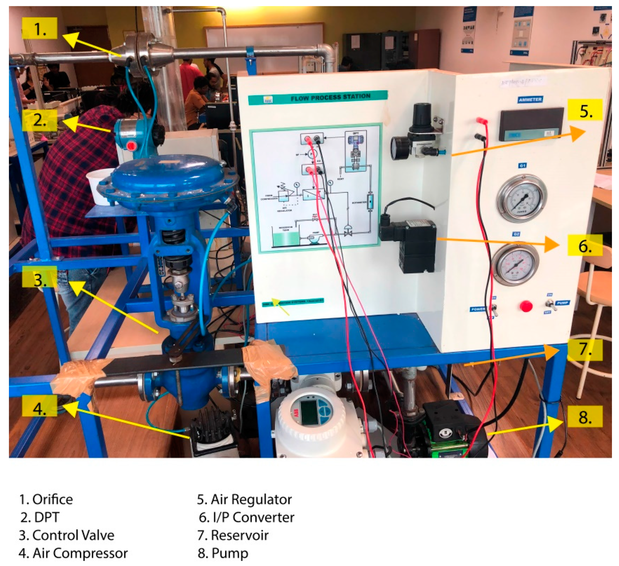
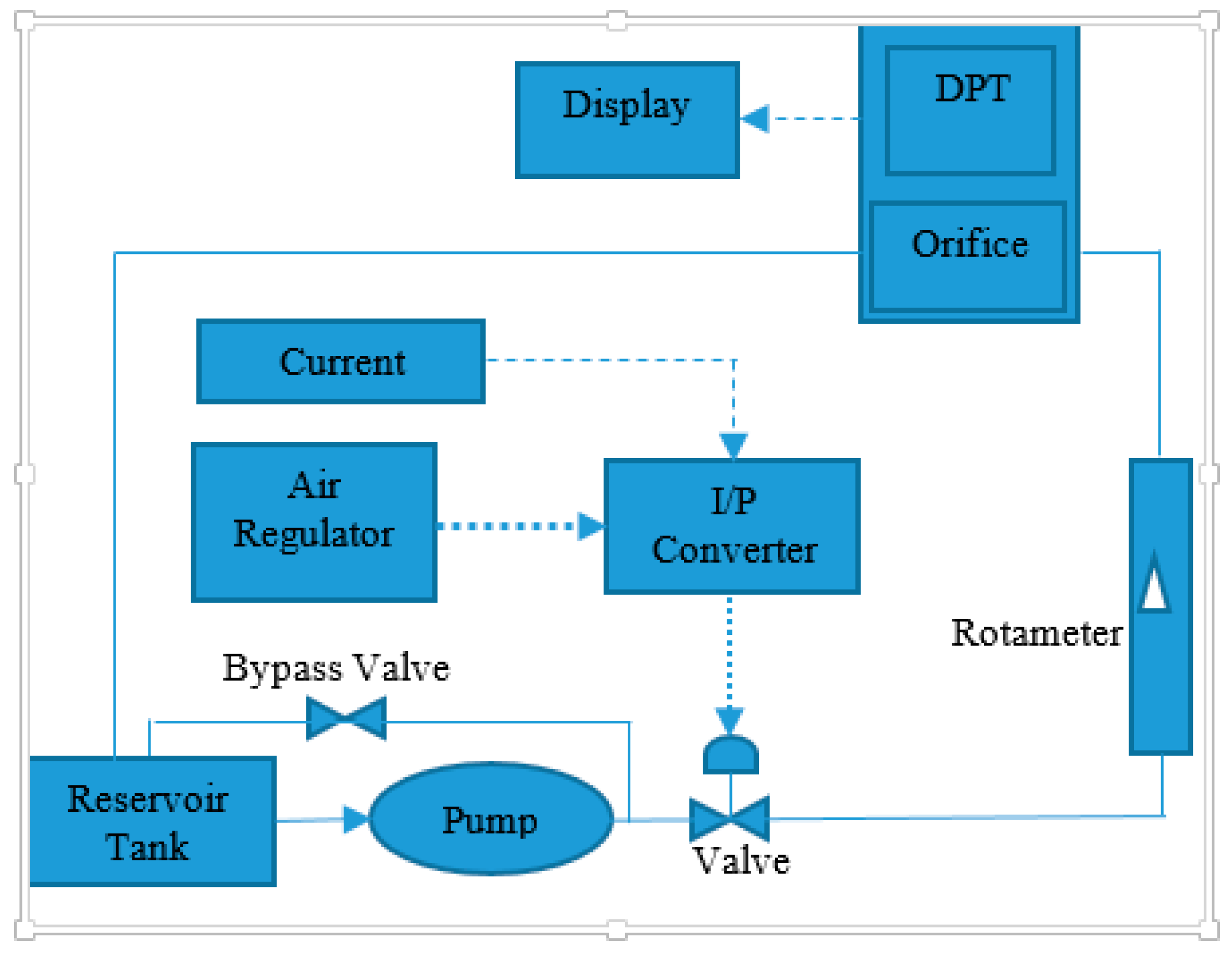
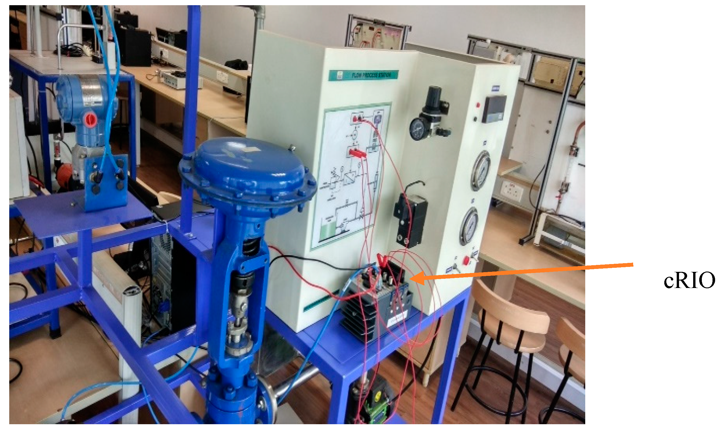
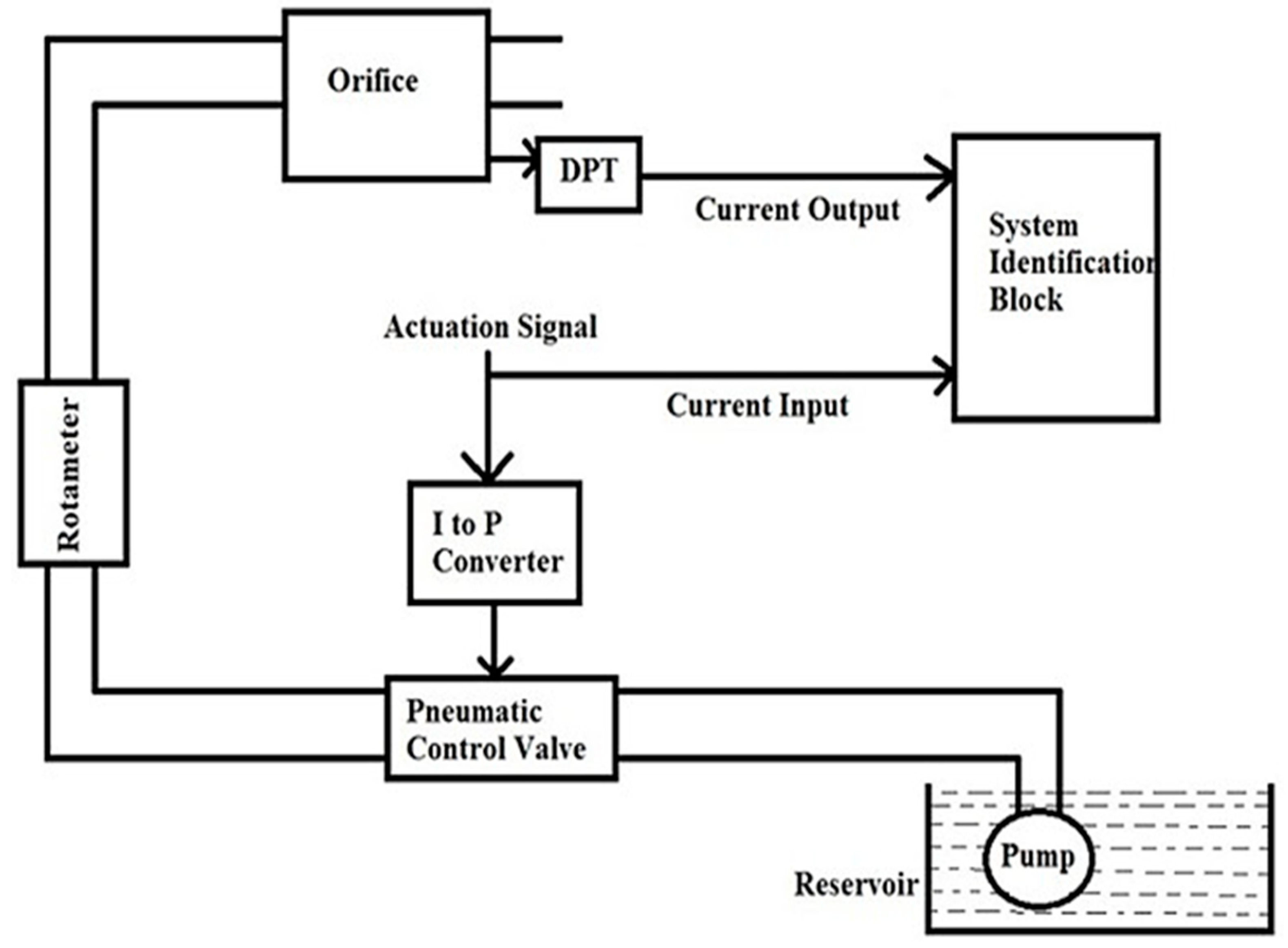
2.1. Flow Process Experimental Setup

Experimental setup for the proposed work is shown in Figure 1. It comprises a motor pump, pneumatic actuator, rotameter, and an orifice flow meter. Water is pumped through a motor pump and is sent through the control valve to the rotameter. Water through the rotameter is directed to the orifice plates and then back to the reservoir. A bypass valve is also provided to create a path for pumped water to flow in case the valve is closed. The pneumatic actuator here used air to open it, and its type and valve position are decided by the pressure applied onto the diaphragm. A piping and instrumentation diagram (P&ID) of the flow process is shown in Figure 2. Dashed lines in the figure indicate the current signal, dotted lines show the air pressure, and solid lines show the fluid flow. Users can give current input of between 4–20 mA to control the valve position, this current is converted into pressure using current to pressure (I/P) converter which gives an output of 3–15 psi. The output from the I/P converter is applied on to the diaphragm, causing a change in the valve position. The orifice creates a change in fluid pressure before and after the plate, and this pressure difference is measured using a differential pressure transmitter which gives an output current of 4–20 mA. This output can be used for further processing or controlling purposes. There is a provision for applying the controller output as an input to the I/P converter to control the valve position. In this work, the aim is to estimate the in-flow rate using a soft sensor in an open loop. A change in the process variable is achieved through manual variation of current input provided to the I/P converter.

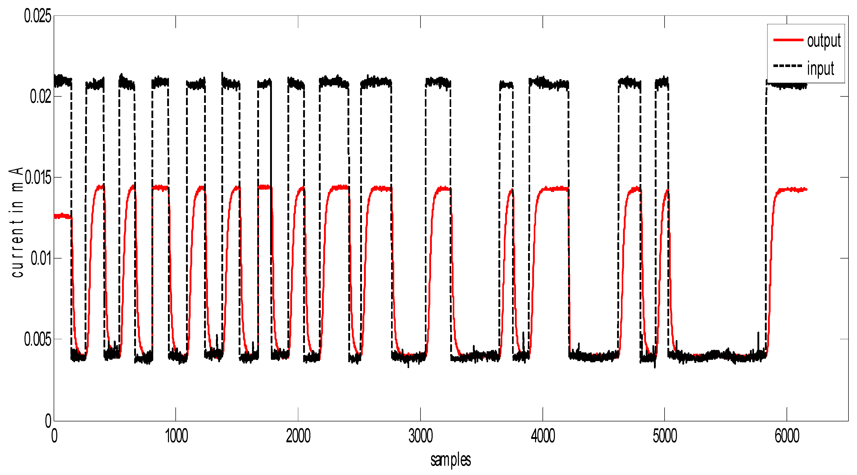
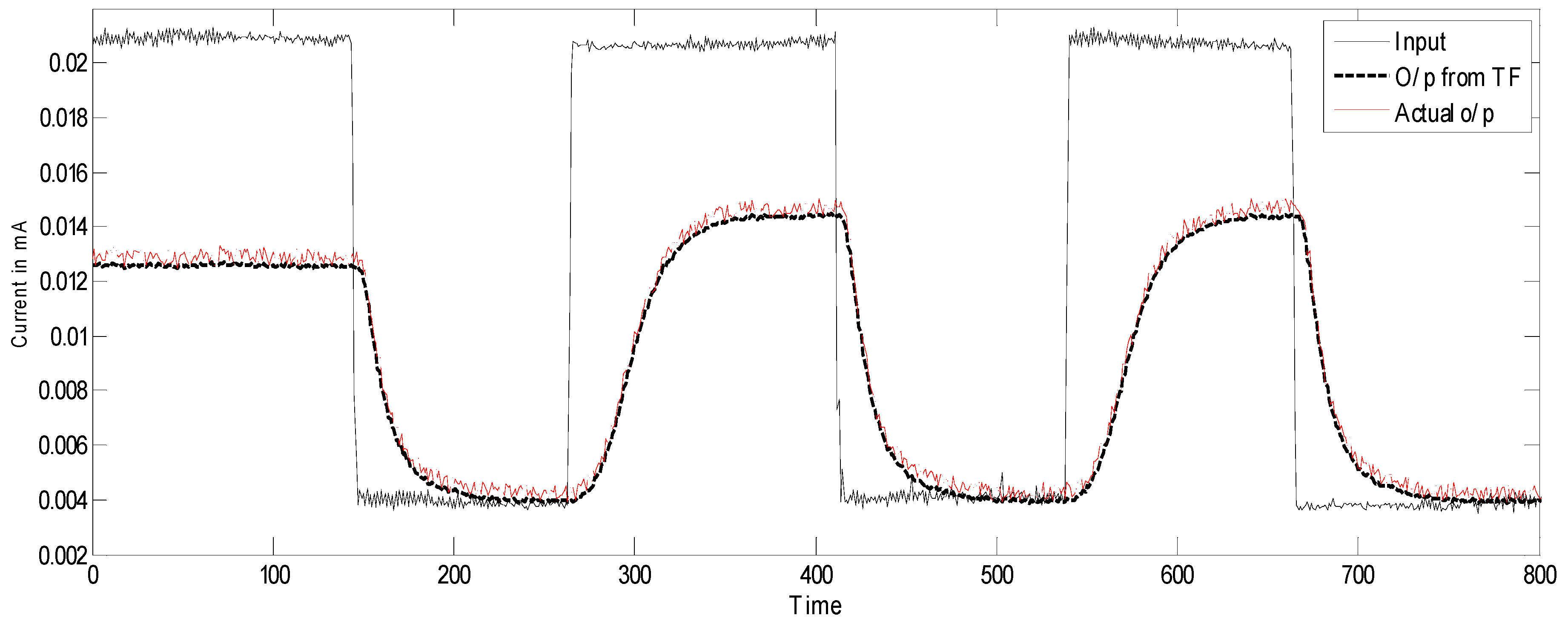
2.2. Identification of the Control Valve Model

In the proposed work, a grey box model identification technique is considered for finding the model of the flow process. A current input signal is used to drive the actuator to vary the flow rate at the outlet of the actuator. The first stage of the model derivation is to get input and output. The data is acquired on a real-time target board (cRIO 9012) through the current input module NI 9203, as shown in Figure 3. NI c-RIO 9012 has chassis consisting of 4 slots for connecting up to 4 input-output modules. NI 9203 is mounted onto the chassis of the c-RIO as shown in Figure 4. This current input module can be interfaced for up to 8 different channels simultaneously. Once the c-RIO is powered, it is interfaced to the PC via an Ethernet cable, while network settings are configured through NI MAX software. Connections are made into the current input module’s channels such that current from the input source to control valve I/P converter and output current from the DPT connected at the orifice are acquired simultaneously.

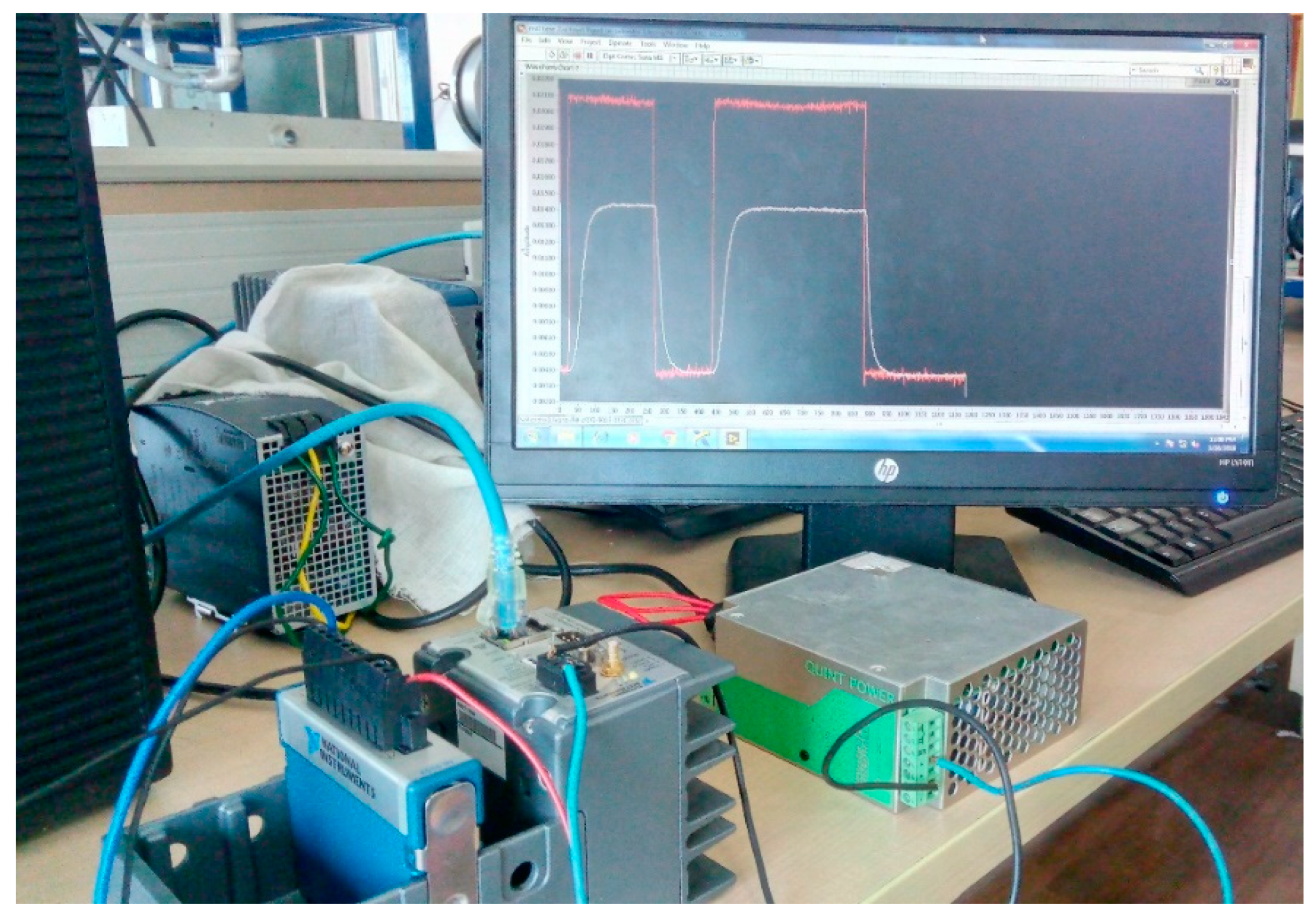
Pseudo Random Signal Response

For analysis, the flow process is assumed to be a first-order system, and the next step is to compute the coefficients of the transfer function. For this computation, the response of the system for a sequence of a step input is considered and the on and off time of the step signal is varied randomly, in order to identify the system to match transit and steady-state behavior. The block diagram in Figure 5 shows the connectivity for the computation of transfer function. The response obtained for the pseudo-random signal is shown in Figure 6.

The first step towards the identification of the transfer function is to examine the trends and select the model structure. From the trends, it can be assumed that the given model replicates the behavior of a first-order system. An adaptive Gauss-Newton search algorithm is used for system identification. The system response can be given by Equation (1)

$$C_f\left(s\right)=G\left(s\right)C_a\left(s\right)+b\left(s\right)$$

(1)

where,

$C_f\left(s\right)$—is the Laplacian of the current signal derived from the DPT

$C_a\left(s\right)$—is the Laplacian of the actuation current signal to the actuator.

$G\left(s\right)$—is the identified transfer function

$b\left(s\right)$—is the Laplacian of the disturbance, which is treated to be almost null in the proposed work.

G(s) is assumed to be of the form K/1+τs. The next step is to identify the values of the coefficients K and τ. A structured parameterization technique is incorporated to compute the coefficients. In this technique, an initial value is assumed and the iterative search algorithm is used to compute the local minima value. The derived transfer function model, keeping the matching index at around 95%, is given in Equation (2):

$$G\left(s\right)= \frac{0.396}{\left(1+0.656s\right)}{e}^{-0.12s}$$

(2)

On the application of Pade’s approximation, the transfer function obtained is

$$G\left(s\right)= \frac{6.6-0.396s}{\left(16.67+11.93s+0.656S^2\right)}$$

(3)

Converting the transfer function to the state-space model we get

$$\begin{gathered} A=\left[\begin{array}{cc}-18.186& -25.4116\\ 1& 0\end{array}\right] \\ B=\left[\begin{array}{c}1\\ 0\end{array}\right] \\ C=\left[\begin{array}{cc}-0.6037& 10.061\end{array}\right] \\ D=\left[0\right] \end{gathered}$$

From the above response in Figure 7, it can be seen that the designed model is able to track the behavior of the physical system. This is followed by designing an observer to estimate the inflow from the derived model.

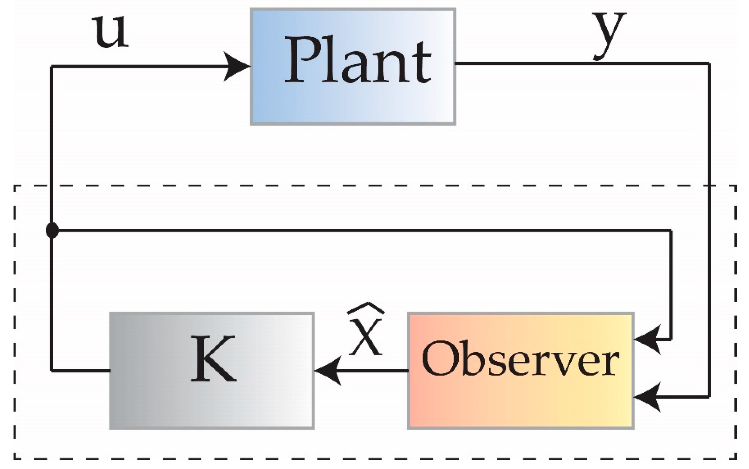
3. Design of Observers

An observer is a model that is used in place of a physical sensor when a physical sensor cannot be placed due to several reasons like non-availability of a sensor, economic constraints, placement constraints, etc. Therefore, observers are also termed soft sensors. In other words, the observer estimates the unknown state variable from the measurement of outputs for a given period [39,40].

For the computation of observers, the first step is to convert the plant model to state-space form. As the derived transfer function has a delay element, Pade approximation is used to convert it into a normal transfer function model. A first-order Pade approximation is used, thus making the plant model a second-order model. Several, observer design methods are reported in the literature, of which the Pole placement technique, Luenberger, Kalman filter, and neural network-based observers are the most common methods [39]. In the proposed work, pole placement and Kalman filter techniques are used for estimation of inflow to the control valve. Pole placement technique is used due to its simplicity and support in achieving the desired system response. Kalman filter is used due to its capacity to provide a fine estimate.

3.1. Pole Placement Technique

Block diagram of the pole placement method of observer design is given in Figure 8 [41]. Pole placement observer is designed based on the principle of feedback estimation, i.e., error, e (t) → 0, as time ‘t’ → ∞; for state $x\left(t\right)-x^{\prime }\left(t\right)=e\left(t\right)$ where $x^{\prime }\left(t\right)$ is the estimate.

Accordingly, the feedback correction is $L\left(y-y^{\prime }\right)$, the objective of the design would be to compute ‘$L$’ such that estimator poles are placed in the proper position.

The equation considering the plant is:

$${\sigma }_x=Ax+Bu,y=Cx+Du$$

(4)

The equivalent considering the observer is:

$${\sigma }_x^{\prime }=A{x}^{\prime }+Bu-L\left(y-C{x}^{\prime }-Du\right)$$

(5)

The equivalent considering the state feedback controller is:

$$u=kx\prime$$

(6)

Using Equations (5) and (6), the observer matric ‘L’ is computed. In the proposed system:

$$L=\left[\begin{array}{cc}0.1& -0.283\\ -0.34& 0\end{array}\right]$$

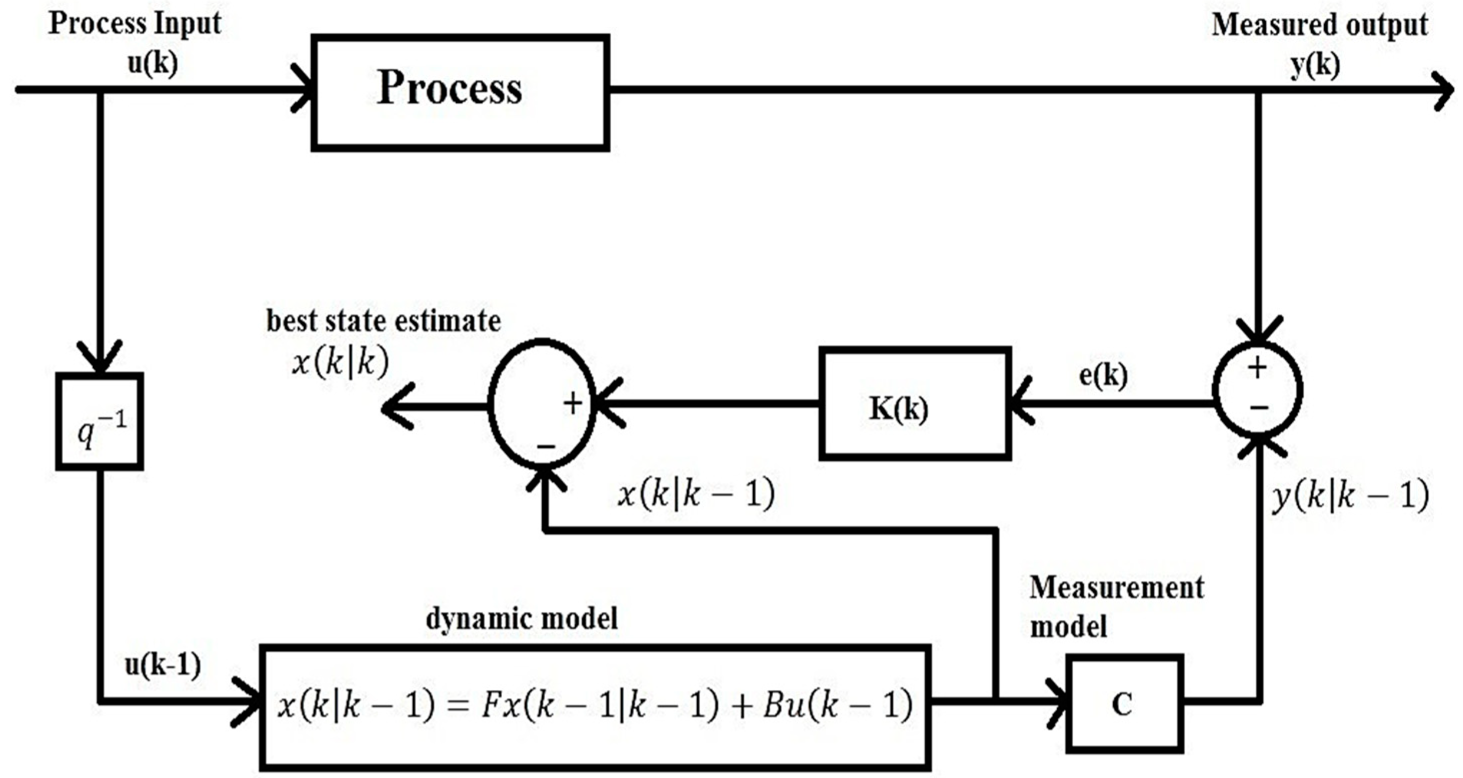
3.2. Kalman Filter Technique

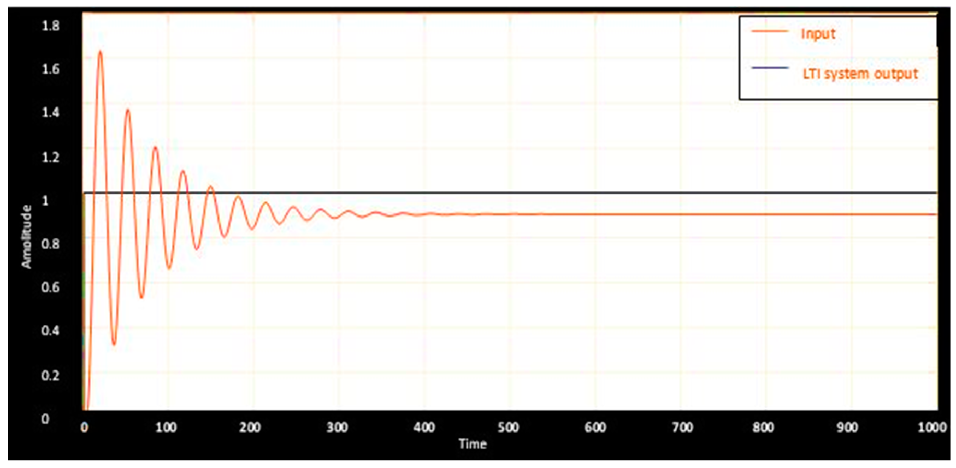
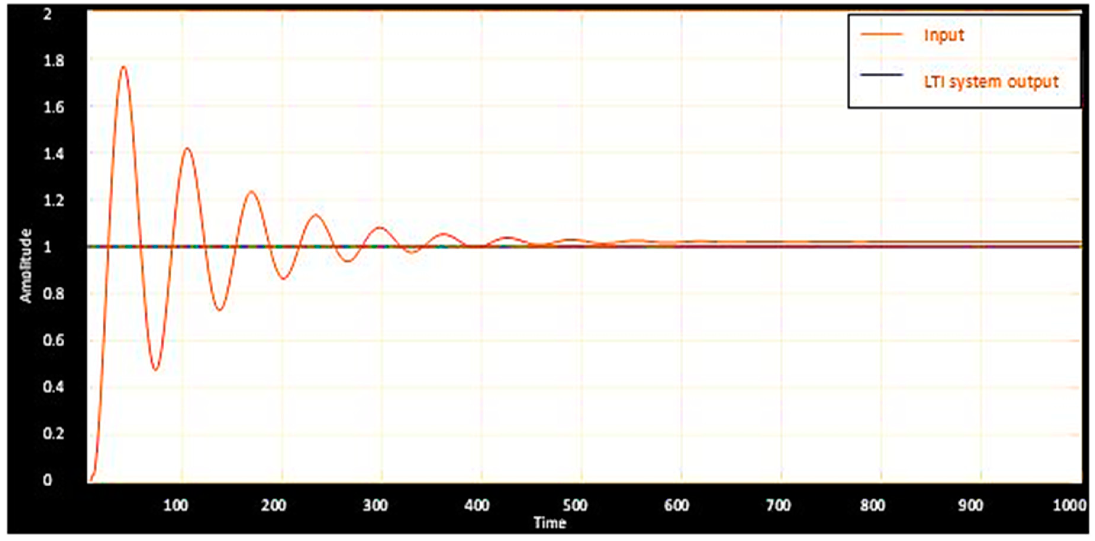
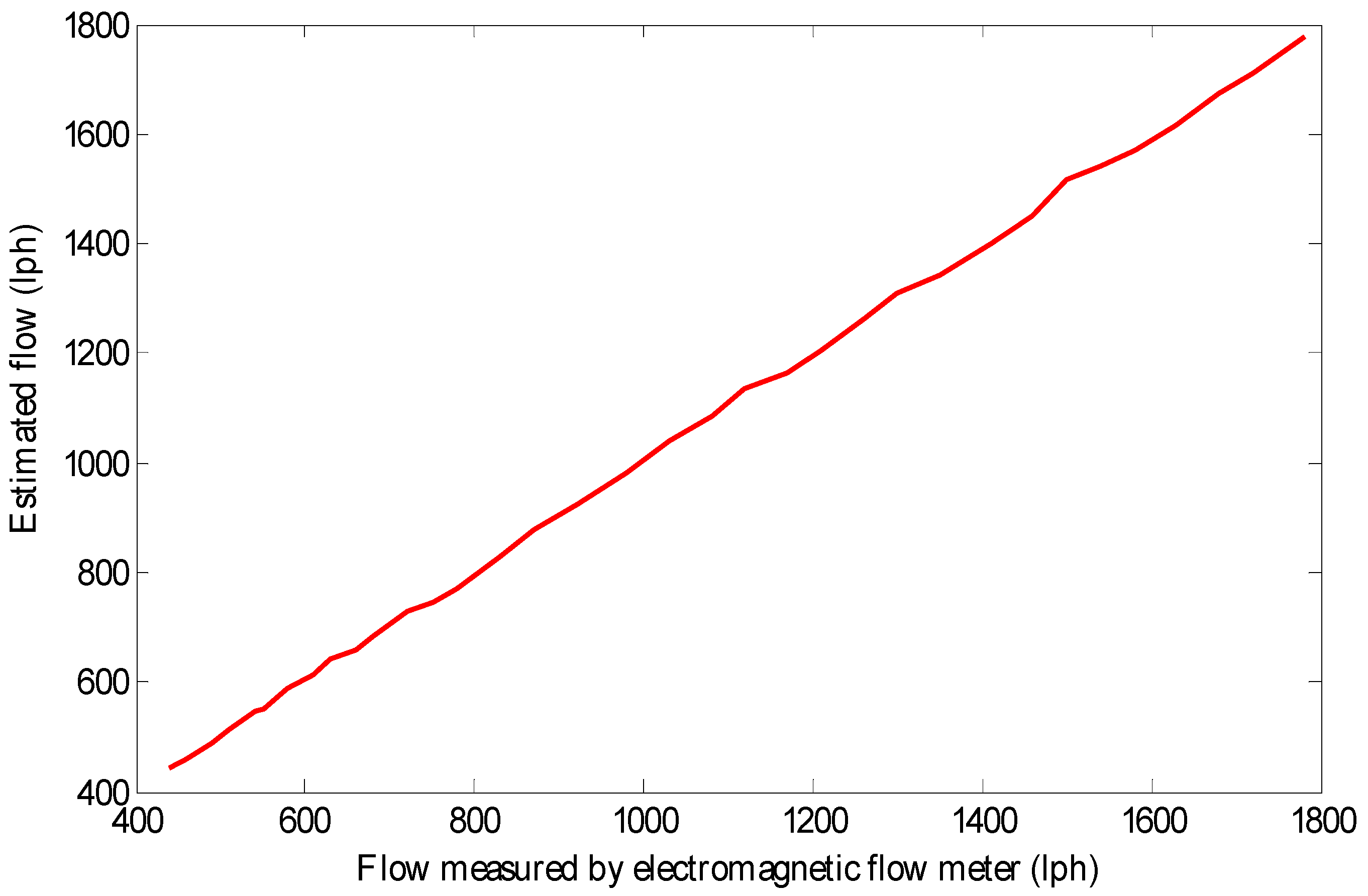
The Kalman filter technique is based on recursive predictive algorithms as shown in Figure 9, which requires the estimated state from the previous time and the current measurement for computation of current stage values [42]. The filter has two variables: ‘a posteriori state estimate (x’k|k) and ‘posteriori error covariance matrix (P’k|k)’. For computation, the system is converted into a discrete domain, and the plant is represented by Equations (7) and (8):

$$X_{k+1}=F_k{X}_k+B_k{u}_k$$

(7)

$$Z_{k+1}=H_{k+1}{X}_{k+1}+V_{k+1}$$

(8)

where ‘$Z_k$’ is the observation at time k, ‘$F_k$’ is the state transition matrix, ‘$B_k$’ is the input matrix, ‘$Q_k$’ is the covariance of process noise. ‘$H_k$’ is the observation matrix, and ‘Vk’ is the observation noise.

Two stages are considered under the Kalman filter technique, the first being the time update (prediction) stage and the second being a measurement update (correction) stage. First, the predict phase $P_{\left(k|k-1\right)}$ is calculated using a state transition matrix ($F_k$), input matrix ($B_k)$and process noise variance matrix ($Q_k$) using the model. In the update phase, we calculate $S_k$ using $H_k$ and$R_k$, which are obtained from the model.

The predicted state estimate is calculated using Equation (9):

$$X_{\left(k|k-1\right)}^{\prime }=F_k{X}_{\left(k-1|k-1\right)}^{\prime }+B_k{U}_k$$

(9)

The predicted estimate covariance is found by using Equation (10):

$$P_{\left(k|k-1\right)}=F_k.P_{\left(k-1|k-1\right)}{F}_k^T+Q_k$$

(10)

The measurement residue is calculated using Equation (11):

$$Y_k^{\prime }=Z_k-H{X}_{\left(k|k-1\right)}^{\prime }$$

(11)

Residual covariance is found using Equation (12):

$$S_k=H_k{P}_{\left(k|k-1\right)}{H}_k^T+R_k$$

(12)

Optimal Kalman gain is obtained using Equation (13):

$$K_k=P_{\left(k|k-1\right)}{H}_k^T{S}_k^{-1}$$

(13)

For the proposed work, computed residues are ${\mathit{S}}_{\mathit{k}}=[\mathbf{0.001} \mathbf{0.0036}]$, ${\mathit{H}}_{\mathit{k}}=[\mathbf{0.001} \mathbf{0.4035}]$.

Both the observers were compared under a simulation test for identifying the better technique for measurement of inflow. The primary test was conducted to evaluate the step response. For comparison of two observer design methods, three performance measures, namely Integral Absolute Error (IAE), Integral Squared Error (ISE), and Integral Time-weighted Absolute Error (ITAE) were used. IAE, ISE and ITAE are mainly used for checking the overall performance of technique with different purposes. ISE reduces the lower range errors whereas higher errors will worsen, as the square of larger error will be high. IAE gives an absolute error integrate and does not affect any of the errors much, but reduces the response time. ITAE reduces errors that persist for a longer duration by integrating them with time.

Figure 10 and Figure 11 show the step response characteristics of the designed observer indicated by the pole placement and the Kalman filter method, respectively. Characteristics showed smooth tracking in the observer using a Kalman filter as compared to that of a pole placement method. In addition, the error produced in measurement are analyzed and the results obtained are shown in

Table 2. Performance errors.

	Kalman Filter Observer	Pole Placement
IAE	0.4896	0.165
ISE	0.038	0.053
ITAE	6.732	11.745

. From the table, it is validated that the Kalman filter based observer is better when compared to that designed by the pole placement technique. Kalman-filter based observer is considered and is subjected to test on a real-life system. For a practical test, the observer is expected to compute the inflow to the actuator, and the response of the observer is the actuating current. The current signal is mapped to the inflow by the use of a normalization constant, which was used earlier while finding the plant model.

The response of estimated flow with the actual flow has a linear characteristic as represented in Figure 12. Actual and estimated values of inflow rate have been presented in

Table 3. Results obtained for input-output testing.

Actual Flow Rate (lph)	Estimated Flow Rate (lph)	Percentage Error
440	442	−0.45
460	459	0.22
490	489	0.20
510	513	−0.59
540	548	−1.48
550	552	−0.36
580	588	−1.38
610	613	−0.49
630	642	−1.90
660	657	0.45
680	684	−0.59
720	728	−1.11
750	744	0.80
780	772	1.03
830	827	0.36
870	877	−0.80
920	926	−0.65
980	984	−0.41
1030	1041	−1.07
1080	1087	−0.65
1120	1134	−1.25
1170	1163	0.60
1210	1204	0.50
1260	1265	−0.40
1300	1309	−0.69
1350	1342	0.59
1410	1400	0.71
1460	1452	0.55
1500	1517	−1.13
1540	1543	−0.19
1580	1572	0.51
1630	1616	0.86
1680	1673	0.42
1720	1711	0.52
1780	1776	0.22

. From Table 3, it is seen that the reported system could estimate the inflow accurately with a maximum deviation of 17 lph, which is about 1.2% of the full-scale range. Accuracy of the designed estimation technique is assessed with reference to the root mean square of percentage error, which is 0.79%.

In order to check the working of the proposed method in closed loop, a PI controller with a proportional gain of 5 and integral gain of 4 was designed for the system. The response of the controller for various step change is highlighted in Figure 13. The percentage error between the estimated value and the actual value has been denoted in Figure 14.

4. Results

Tests were conducted on a computed Kalman filter based observer model to understand its performance in real life. Water was pumped to the process using a motor; the valve position is varied to produce changes in the flow rate of water. The flow rate is varied in the ranges of 400 lph to 1800 lph. Estimated inflow from the measured outflow using orifice flow meter is given in Table 3. The estimated inflow is compared with the actual inflow, which is measured using a standard electromagnetic flow meter.

The proposed estimation method is compared with a neural network using a nonlinear autoregressive exogenous method. In reference [4], the flow rate in m3/h was estimated on an hourly basis for performance measures tabulated in

Table 4. Comparison of performance parameters.

Parameters	Proposed Method Using Kalman Filter	Nonlinear Autoregressive Exogenous Model Reported in Reference [4]
MAE	8.6 × 10−4	0.2041
MSE	5.96 × 10−5	0.1111
RMSE	0.0077	0.3332

. As in reference [4] flow rate was given in m³/h, measurements of proposed technique are also converted from lph to m3/h. After conversion, three performance parameters: mean absolute error (MAE), mean square error (MSE) and root-mean-square error (RMSE) were calculated and have been compared with the results of reference [4]. From Table 4, the proposed technique shows better performance compared with the results of reference [4].

5. Conclusions

Control of flow has always been one of the most widely carried out processes in industries. Placement of flow meters is always a critical and challenging task, as the flow meter cannot be placed at all locations. For measurement of flow at those locations, we will need to design an estimator/soft sensor. The reported work aims at designing such a technique to measure the inflow to the control valve by measuring flow at the outlet of a control valve. Estimation algorithms are driven by the signal acquired from sensors, in this case, a flowmeter.

The reported paper is designed with the help of an observer to identify the inflow. Pole placement technique and Kalman filter techniques were used to design the observer. After the output obtained from both the observers in the simulation, the results showed the Kalman filter to be better compared to the pole placement technique. Practical test results of the Kalman filter also showed a successful implementation of the estimation technique. Proposed Kalman filter method results were compared with the estimation technique used in reference [4], resulting in much lower MAE, MSE, and RMSE values. This method was able to give a root-mean-square percentage error of around 0.79%, leading to higher accuracy with a lower deviation of estimated values. From the analysis of characteristics and accuracy performance, it is seen that the designed soft sensor can be used in practical applications.

References

1. Shah, M.S.; Joshi, J.B.; Kalsi, A.S.; Prasad, C.S.; Shukla, D.S. Analysis of flow through an orifice meter: CFD simulation. Chem. Eng. Sci. 2012, 26, 300–309. [Google Scholar] [CrossRef]
2. Bentley, J.P. Principles of Measurement Systems; Pearson Education: London, UK, 2005. [Google Scholar]
3. Manshoor, B.B.; Nicolleau, F.C.; Beck, S.B. The fractal flow conditioner for orifice plate flow meters. Flow Meas. Instrum. 2011, 22, 208–214. [Google Scholar] [CrossRef]
4. Haddad, S.; Benghanem, M.; Mellit, A.; Daffallah, K.O. ANNs-based modeling and prediction of hourly flow rate of a photovoltaic water pumping system: Experimental validation. Renew. Sustain. Energy Rev. 2015, 1, 635–643. [Google Scholar] [CrossRef]
5. Norgia, M.; Pesatori, A.; Donati, S. Compact laser-diode instrument for flow measurement. IEEE Trans. Instrum. Meas. 2016, 65, 1478–1483. [Google Scholar] [CrossRef]
6. Liu, W.; Hu, J.; Zhao, X.; Pan, H.; Lakhiar, I.A.; Wang, W. Development and experimental analysis of an intelligent sensor for monitoring seed flow rate based on a seed flow reconstruction technique. Comput. Electron. Agric. 2019, 164, 104899. [Google Scholar] [CrossRef]
7. Arlit, M.; Schroth, C.; Schleicher, E.; Hampel, U. Flow rate measurement in flows with asymmetric velocity profiles by means of distributed thermal anemometry. Flow Meas. Instrum. 2019, 68, 101570. [Google Scholar] [CrossRef]
8. Langford, S.; Wiggins, C.; Tenpenny, D.; Ruggles, A. Positron emission particle tracking (PEPT) for fluid flow measurements. Nucl. Eng. Des. 2016, 302, 81–89. [Google Scholar] [CrossRef]
9. Venkata, S.K.; Roy, B.K. A practically validated intelligent calibration circuit using optimized ANN for flow measurement by venture. J. Inst. Eng. Ser. B 2016, 97, 31–39. [Google Scholar] [CrossRef]
10. Kim, Y.S. Overview of geometrical effects on the critical flow rate of sub-cooled and saturated water. Ann. Nucl. Energy 2015, 76, 12–18. [Google Scholar] [CrossRef]
11. Lannes, D.P.; Gama, A.L.; Bento, T.F. Measurement of flow rate using straight pipes and pipe bends with integrated piezoelectric sensors. Flow Meas. Instrum. 2018, 60, 208–216. [Google Scholar] [CrossRef]
12. Lay-Ekuakille, A.; Vergallo, P.; Griffo, G.; Morello, R. Pipeline flow measurement using real-time imaging. Measurement 2014, 47, 1008–1015. [Google Scholar] [CrossRef]
13. Sinha, S.; Banerjee, D.; Mandal, N.; Sarkar, R.; Bera, S.C. Design and implementation of real-time flow measurement system using Hall probe sensor and PC-based SCADA. IEEE Sens. J. 2015, 15, 5592–5600. [Google Scholar] [CrossRef]
14. Hussain, A.; Ahmad, Z.; Ojha, C.S. Flow through lateral circular orifice under free and submerged flow conditions. Flow Meas. Instrum. 2016, 52, 57–66. [Google Scholar] [CrossRef]
15. Schena, E.; Cecchini, S.; Silvestri, S. An orifice meter for bidirectional air flow measurements: Influence of gas thermo-hygrometric content on static response and bidirectionality. Flow Meas. Instrum. 2013, 34, 105–112. [Google Scholar] [CrossRef]
16. Peters, F.; Groß, T.F. Flow rate measurement by an orifice in a slowly reciprocating gas flow. Flow Meas. Instrum. 2011, 22, 81–85. [Google Scholar] [CrossRef]
17. Shan, F.; Liu, Z.; Liu, W.; Tsuji, Y. Effects of the orifice to pipe diameter ratio on orifice flows. Chem. Eng. Sci. 2016, 152, 497–506. [Google Scholar] [CrossRef]
18. Jaiswal, S.K.; Yadav, S.; Agarwal, R. Design and development of a novel water flow measurement system. Measurement 2017, 105, 120–129. [Google Scholar] [CrossRef]
19. Edwards, J.E.; Otterson, D.W. Tech Talk (6) Flow Measurement Basics (Part 1). Meas. Control 2015, 48, 18–25. [Google Scholar] [CrossRef]
20. Xing, L.; Hua, C.; Zhu, H.; Drahm, W. Flow Measurement Model of Ultrasonic Flowmeter for Gas-Liquid Two-Phase Stratified and Annular Flows. Adv. Mech. Eng. 2014, 6, 194871. [Google Scholar] [CrossRef]
21. Wang, X.; Sun, X.; Doup, B.; Zhao, H. Dynamic modeling strategy for flow regime transition in gas-liquid two-phase flows. J. Comput. Multiph. Flows 2012, 4, 387–397. [Google Scholar] [CrossRef]
22. Medeiros, K.A.; de Oliveira, F.L.; Barbosa, C.R.; de Oliveira, E.C. Optimization of flow rate measurement using piezoelectric accelerometers: Application in water industry. Measurement 2016, 91, 576–581. [Google Scholar] [CrossRef]
23. Yan, Y.; Wang, L.; Wang, T.; Wang, X.; Hu, Y.; Duan, Q. Application of soft computing techniques to multiphase flow measurement: A review. Flow Meas. Instrum. 2018, 60, 30–43. [Google Scholar] [CrossRef]
24. Tsukada, K.; Kikura, H. Study on Velocity Profile Measurement of Saturated Jet Flow by Air-coupled Ultrasound. Energy Procedia 2017, 131, 436–443. [Google Scholar] [CrossRef]
25. Krejčí, J.; Ježová, L.; Kučerová, R.; Plička, R.; Broža, Š.; Krejčí, D.; Ventrubová, I. The measurement of small flow. Sens. Actuators A Phys. 2017, 266, 308–313. [Google Scholar] [CrossRef]
26. Boushaki, T.; Koched, A.; Mansouri, Z.; Lespinasse, F. Volumetric velocity measurements (V3V) on turbulent swirling flows. Flow Meas. Instrum. 2017, 54, 46–55. [Google Scholar] [CrossRef]
27. Li, Q.; Xing, J.; Shang, D.; Wang, Y. A Flow Velocity Measurement Method Based on a PVDF Piezoelectric Sensor. Sensors 2019, 19, 1657. [Google Scholar] [CrossRef]
28. Formato, G.; Romano, R.; Formato, A.; Sorvari, J.; Koiranen, T.; Pellegrino, A.; Villecco, F. Fluid–Structure Interaction Modeling Applied to Peristaltic Pump Flow Simulations. Machines 2019, 7, 50. [Google Scholar] [CrossRef]
29. Chen, S.; Yu, M.; Kan, J.; Li, J.; Zhang, Z.; Xie, X.; Wang, X. A Dual-Chamber Serial–Parallel Piezoelectric Pump with an Integrated Sensor for Flow Rate Measurement. Sensors 2019, 19, 1447. [Google Scholar] [CrossRef]
30. Silva, W.L.; Lima, V.S.; Fonseca, D.A.; Salazar, A.O.; Maitelli, C.W.; Echaiz, E.; German, A. Study of Flow Rate Measurements Derived from Temperature Profiles of an Emulated Well by a Laboratory Prototype. Sensors 2019, 19, 1498. [Google Scholar] [CrossRef]
31. Rad, C.R.; Hancu, O. An improved nonlinear modelling and identification methodology of a servo-pneumatic actuating system with complex internal design for high-accuracy motion control applications. Simul. Model. Pract. Theory 2017, 75, 29–47. [Google Scholar] [CrossRef]
32. Metwally, M.; Aly, A.A.; Ola, M. Effect of spool side chambers on dynamic response of contactless electro-operated pneumatic directional control valve. Comput. Fluids 2013, 86, 125–132. [Google Scholar] [CrossRef]
33. Topçu, E.E.; Yüksel, İ.; Kamış, Z. Development of electro-pneumatic fast switching valve and investigation of its characteristics. Mechatronics 2006, 16, 365–378. [Google Scholar] [CrossRef]
34. Li, S.; Wu, P.; Cao, L.; Wu, D.; She, Y. CFD simulation of dynamic characteristics of a solenoid valve for exhaust gas turbocharger system. Appl. Therm. Eng. 2017, 110, 213–222. [Google Scholar] [CrossRef]
35. Tlisov, A.A.; Mitrishkin, Y.V. Adaptive control system for pipeline valve pneumatic actuator. IFAC Proc. Vol. 2009, 42, 373–378. [Google Scholar] [CrossRef]
36. Chinyaev, I.R.; Fominykh, A.V.; Pochivalov, E.A. Method for Determining of the Valve Cavitation Characteristics. Procedia Eng. 2016, 150, 260–265. [Google Scholar] [CrossRef] [Green Version]
37. Righettini, P.; Giberti, H.; Strada, R. A novel in field method for determining the flow rate characteristics of pneumatic servo axes. J. Dyn. Syst. Meas. Control 2013, 135, 041013. [Google Scholar] [CrossRef]
38. Wang, T.; Zhao, L.; Zhao, T.; Fan, W.; Kagawa, T. Determination of Flow Rate Characteristics for Pneumatic Components During Isothermal Discharge by Integral Algorithm. J. Dyn. Syst. Meas. Control 2012, 134, 061005. [Google Scholar] [CrossRef]
39. Fortuna, L.; Graziani, S.; Rizzo, A.; Xibilia, M.G. Soft Sensors for Monitoring and Control of Industrial Processes; Springer-Verlag: London, UK, 31 May 2007. [Google Scholar]
40. Pappalardo, C.; Guida, D. System identification algorithm for computing the modal parameters of linear mechanical systems. Machines 2018, 6, 12. [Google Scholar] [CrossRef]
41. Astrom, K.J.; Murray, R.M. Feedback Systems: An Introduction for Scientists and Engineers; Princeton University Press: New Jersey, NJ, USA, 2010; pp. 201–219. [Google Scholar]
42. Grewal, M.S. Kalman Filtering; Springer: Berlin/Heidelberg, Germany, 2011; pp. 705–708. [Google Scholar]
Figure 1. Experimental Setup.
Machines 07 00063 g001
Figure 2. Piping and instrumentation diagram (P&ID) of flow process.
Machines 07 00063 g002
Figure 3. Setup connected through real-time target board (cRIO).
Machines 07 00063 g003
Figure 4. cRIO with NI 9203 connected to the computer.
Machines 07 00063 g004
Figure 5. Block diagram of identification block.
Machines 07 00063 g005
Figure 6. Response plot used for identification.
Machines 07 00063 g006
Figure 7. The response of the actual system and estimated transfer function.
Machines 07 00063 g007
Figure 8. Block diagram of an observer using pole placement.
Machines 07 00063 g008
Figure 9. Block diagram of an observer using a Kalman filter.
Machines 07 00063 g009
Figure 10. Estimation using pole placement observer for a step signal.
Machines 07 00063 g010
Figure 11. Estimation using Kalman filter for a step signal.
Machines 07 00063 g011
Figure 12. Input-output characteristics of the proposed technique.
Machines 07 00063 g012
Figure 13. Controller response.
Machines 07 00063 g013
Figure 14. Error characteristics of the proposed technique.
Machines 07 00063 g014