Field Programmable Gate Array-Based Linear Shaft Motor Drive System Design in Terms of the Trapezoidal Velocity Profile Consideration

Abstract

Owing to the benefits of programmable and parallel processing of the field programmable gate arrays (FPGAs), they have been widely used to the realization of digital controllers and motor drive systems. In this study, we adopt the FPGA chip to realize the Linear Shaft Motor (LSM) drive system which includes the position, speed and current vector controls. Linear shaft motor is a special motor which has the magnet as the shaft and stator coils are on the forcer. Thus, it reveals a small mechanical time constant. In addition, the electrical side can be looked as a general three-phase Alternating Current (AC) system which can be powered by inverter and vector control technique can be applied to the system. The designed system needs high performance calculation ability about position/speed control and vector current control loops. The mathematical model of linear shaft motor drive system is first built and simulated by MATLAB/Simulink and the accuracy about the effect from the speed estimation method is proposed. The resulting digital model of the drive system is stored into Verilog Hardware Description Language (Verilog HDL) codes and realized by FPGA. At last, the hardware circuits as well as the power module are used to test the performance of the developed hardware system in terms of the trapezoidal velocity profile. The experimental results show that the designed system realized by FPGA has attained the desired performance.

1. Introduction

Linear motors of various types have been developed and investigated [1,2,3,4,5,6,7,8,9,10,11]. A shaft motor is a type of permanent magnet (PM) linear motor that consists of only windings and a non-magnetic pipe filled with PMs [1,4,6,7]. Simplification of the mechanism and light weighting of the forcer are the advantages of shaft motors. Besides, it also has several other advantages, such as direct drive, no backlash, high speed, high precision, small speed chopping, long stroke and support for multi-slide platform. Motion system driven by linear shaft motor has the benefit of no the backlash as comparing to the traditional ball screw plus rotating motor system. It can not only meet the higher speed requirement than the traditional ball screw-based motion system but also run smoothly at low speed, which can meet the long stroke demand that cannot be achieved by the general ball screw platform.

For AC motor drive control system, due to the development of vector control, the three-phase currents can be transformed into a two-axis rotating direct current (Park’s Transformation) via coordinate transformation, which can make the electromagnetic force of the motor proportional to the quadrature component [4,5,10,12,13,14,15,16]. This type control structure is proportional to the control of the conventional brush-type DC motor. Through the feedback of q-axis current, the linear shaft motor can achieve more precise control performances, such that it can be high-speed light-load automation equipment and operated in dust-free environment. However, the light weight of the forcer of the linear shaft motor causes the mechanical time constant being small, it thus needs a fast sampling frequency to make the system stable and be operated properly. The traditional concept of mechanical time constant is about ten times the electric time constant and the transfer function of inner current loop can be looked as constant. However, in both the loops, the sampling frequency of the mechanical loop is as fast as the electrical control loop.

Field programmable gate arrays (FPGAs) are fully customizable to the system designer’s requirements. It allows for a completely flexible design and realization for specific types of control technology [2,13,17,18,19] and adapted to any design changes through dynamic reconfiguration. FPGA-based digital control systems have been successfully implemented on Linear Motor [2,5,20], Induction motor (IM) [12,21], Permanent Magnet Synchronous motor (PMSM) [22,23], stepper motor [14,16] and Brushless Direct Current motor (BLDCM) drive system [13]. It is also shown on the motor control system design by combining the Digital Signal Processor (DSP) and FPGA [24]. For a complete motion system, it includes the motion controller and drive system. The motion control can be found in Reference [17]. For the proposed system, not only the drive system design as those similar works mentioned above but also the motion controller to generate the desired velocity profile and position command is included. Their performances are simply demonstrated by showing the trapezoidal speed profile-based control.

A fast motion control system needs a short sampling time for speed and position control loop and the speed feedback is usually from the difference of the accumulated pulse amount per sampling time. A short sampling time causes the speed ripple bigger than a long one and moving average is usually used to smooth the ripple. However, the moving average action is low pass filter which leads to time lag to the speed response. Furthermore, the position control with pulse difference speed feedback may lead to steady-state offset position error which cannot be reduced by integral action control in the cascade position-speed-torque control structure. Thus, a switching control structure which is original from the sliding mode control is used to solve the problem [25]. It is inserted to the system when the motion control system approaches to the steady-state condition. The control algorithm skips the speed and current controllers and the output of the position control loop directly goes to the inverter input to provide the control voltage for the motor.

In this paper, the model of the linear shaft motor is given and the module to be simulated is created by the MATLAB/Simulink where the main considerations are the correctness and performance of the functional block diagram. Next, the parameters of the controllers to the current and speed/position loops are determined. The created overall systems are digitalized with appropriated sampling time for these two control loops. Thereafter, the resulting hardware system is directly converted into Verilog code. With some modifications on the data type for all the controlled variables of the original Verilog system, we have the final hardware circuits in the format of Verilog code. Based on the hardware codes, they are synthesized and simulated by Quartus II and Modelsim. Finally, the hardware system is realized on Altera Cyclone III FPGA and tested on a linear shaft motor platform by step position and trapezoidal speed commands to verify the performance and validness of the designed drive system. In the proposed design, all the systems are realized in the FPGA except the power module and analog phase current conversion, which attains the performance of fully digital design and can easily be combined into an existed Intellectual Property (IP) system. Furthermore, the system is initially developed on the MATLAB/Simulink platform, the block diagram structures allow the designers to easily verify and change their hardware system due to the ability of hardware in line co-simulation, where the resulting hardware code can be looked as an individual block and performs the simulation with pure software system.

The contents of the paper are as follows. In Section 2, the system structure and the built models are introduced. Then, Section 3 demonstrates the simulations and verifications about the established system. Next, Section 4 shows the experimental results and discussions about the trapezoidal profile speed command and the modified system structure with switching control. Finally, some conclusions are given in Section 5.

2. The System Architecture and Modeling

2.1. Transformation Matrix of the Vector Control

For a general AC motor drive system, through the process of decoupling, the mathematical models coupled to each other can be simplified into a linear and completely separated mathematical model like the conventional DC motor that the desired torque can be obtained by controlling the quadrature component and keeping the direct component constant.

Linear shaft motor has a three-phase power system on the forcer and the permanent magnet is on its shaft. The system can be looked as a three-phase permanent magnet synchronous motor system by changing the rotation angle and velocity into linear displacement and speed. Thus, the coordinate transformations for a three-phase stationary reference frame system to a two-phase synchronous reference frame system by (1),

$$\left[\begin{array}{c}{i}_{ds}\\ i_{qs}\end{array}\right]=\frac{2}{3}\left[\begin{array}{ccc}cos{\theta }_e& cos({\theta }_e-2\pi /3)& cos({\theta }_e+2\pi /3)\\ -sin{\theta }_e& -sin({\theta }_e-2\pi /3)& -sin({\theta }_e+2\pi /3)\end{array}\right]\left[\begin{array}{c}{i}_{as}\\ i_{bs}\\ i_{cs}\end{array}\right]$$

(1)

where ${\theta }_e$ is the electrical angle referred to the linear position. $i_{as}$, $i_{bs}$ and $i_{cs}$ are the phase currents of the stationary reference frame and $i_{ds}$ and $i_{qs}$ are the corresponding d- and q-axis currents. The inverse matrix operation (2) is used to convert the two-phase synchronous reference frame system into three-phase system.

$$\left[\begin{array}{c}{v}_{as}\\ v_{bs}\\ v_{cs}\end{array}\right]=\left[\begin{array}{cc}cos{\theta }_e& -sin{\theta }_e\\ cos({\theta }_e-2\pi /3)& -sin({\theta }_e-2\pi /3)\\ cos({\theta }_e+2\pi /3)& -sin({\theta }_e+2\pi /3)\end{array}\right]\left[\begin{array}{c}{v}_{ds}\\ v_{qs}\end{array}\right]$$

(2)

Equation (2) is for simulation only and does not used to the realization of hardware drive system.

2.2. Mathematical Model of Linear Shaft Motor

The Equations (3)–(5) are the axial force type electromagnetic equation and Equation (6) is the motor mechanical equation.

$$\frac{d{i}_{ds}}{dt}=-\frac{R_s}{L_s}{i}_{ds}+\frac{1}{L_s}{v}_{ds}+\frac{\pi }{\tau }(\frac{dx}{dt})i_{qs}$$

(3)

$$\frac{d{i}_{qs}}{dt}=-\frac{R_s}{L_s}{i}_{qs}+\frac{1}{L_s}{v}_{qs}-\frac{\pi }{\tau }(\frac{dx}{dt})i_{ds}-\frac{\pi }{\tau }\frac{1}{L_s}(\frac{dx}{dt}){\phi }_F$$

(4)

$$F_e=\frac{\pi }{\tau }(\frac{3}{2}{i}_{qs}{\phi }_F)$$

(5)

$$M\frac{d^{2}x}{d{t}^2}+\beta \frac{dx}{dt}+F_L=F_e$$

(6)

where $i_{ds}$ and $i_{qs}$ are the d- and q-axis currents of the coil on the forcer, $v_{ds}$ and $v_{qs}$ are the d- and q-axis applied voltages, $R_s$ is the resistance, $L_s$ is the inductance, ${\phi }_F$ is the magnetic flux of the shaft, $M$ is the mass of forcer, $\beta$ is the viscous friction coefficient, $\tau$ is the polar distance (North to South), $F_L$ is the load, $F_e$ is the generated electromagnetic thrust, $x$ is the position. The position $x$ is related to the phase angle ${\theta }_e$ as

$${\theta }_e=\frac{\pi }{\tau }x$$

(7)

Equation (7) is used for the look-up table of sin/cos functions.

2.3. Overall System Architecture

The experimental hardware system is shown in Figure 1, it includes the DC power supply, the FPGA-based control board, the power board with MOSFET, the analog to digital converter (ADC) and digital to analog converter (DAC) and the linear shaft motor. The two converters are built on the FPGA board.

The Hall current sensors on the power board detect the currents of phases A and B and the analog current signals are sent to the ADC converter. The serial ADC is operated on 20 MHz clock. The 12-bit digital values of currents are fed back to the digital controller for the Clarke and Park transformations. The d- and q-axis current controllers determine the d- and q-axis voltages to make the stator’s circuits have the response of the desired. The coil voltages, $v_{ds}$ and $v_{qs}$, are generated by the space vector pulse width modulation (SVPWM) technique with working frequency 20 kHz which is also the sampling frequency of the two current digital Proportional-Integral (PI) controllers. As for the speed control, the feedback is from the incremental encoder with resolution 10,000 pulse/cm. Position and speed controllers are also with the PI type and their sampling frequencies are set as 2 kHz since the forcer of the system is quite light such that they have a small mechanical time constant.

Figure 2 is the functional block diagram for the hardware control system. The up/down counter is designed to accept the A/B/Z phase pulse signals from the incremental encoder and outputs a 4-time precision pulse signal for position feedback. The current vector control implements the regulation of d- and q-axis currents, which includes the reference frame transformation and two PI controllers. The sampling frequencies of current controllers are 20 kHz and position and speed controllers are 2 kHz. The position command can be from the motion controller (Pulse Generator) which is made from the FPGA chip as well. The type of command could be step or from a series of pulse which can be trapezoidal or S-shape speed profile. Power module is used to generate 3-phase AC power supply. ADC is used to convert the analog current into digital type for current feedback and DAC is used to convert the digital value in the FPGA into analog type signal for demonstration.

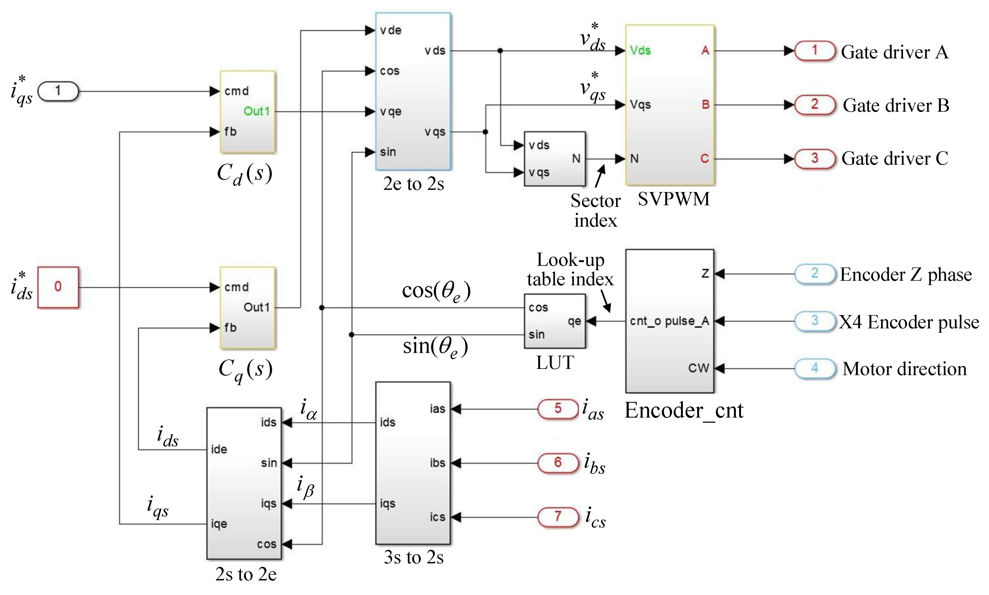
2.4. Digital System Architecture of the Vector Control

Figure 3 is the functional block diagram for the modelling of current vector control of $i_{ds}$ and $i_{qs}$. The block “Encoder_cnt” is used to accumulate the position pulses from the four-time precision circuit. The “Encoder_cnt” outputs the 11-bit index signal named as Look-up table (LUT) index for sin/cos table to get the values, $sin({\theta }_e)$ and $cos({\theta }_e)$, from the “LUT” block for coordinate transformation. Block “3s to 2s” accepts the stator currents, $i_{as}$, $i_{bs}$ and $i_{cs}$ and converts them into the stationary reference frame currents, $i_{\alpha }$ and $i_{\beta }$. Next, by the block “2s to 2e”, $i_{\alpha }$ and $i_{\beta }$ are converted into the two-phase synchronous reference frame currents, $i_{ds}$ and $i_{qs}$, for current feedbacks. The two PI controllers, $C_d(s)$ and $C_q\left(s\right)$, are respectively designed to make the currents to the desired, that is, $i_{ds}^{*}=0$ A and $i_{qs}^{*}$ is proportional to the required force to make the forcer move to the desired position with the speed limitations. The outputs of the current controllers are applied to the “SVPWM” module to generate the gate driver signals, Gate driver A, Gate driver B and Gate driver C, to turn ON or OFF the Metal-Oxide-Semiconductor Field-Effect Transistors (MOSFETs) or Insulated Gate Bipolar Transistors (IGBTs) switches. The data format for the designed system is based on a 32-bit system where the integer part and fractional part will be shown in later section.

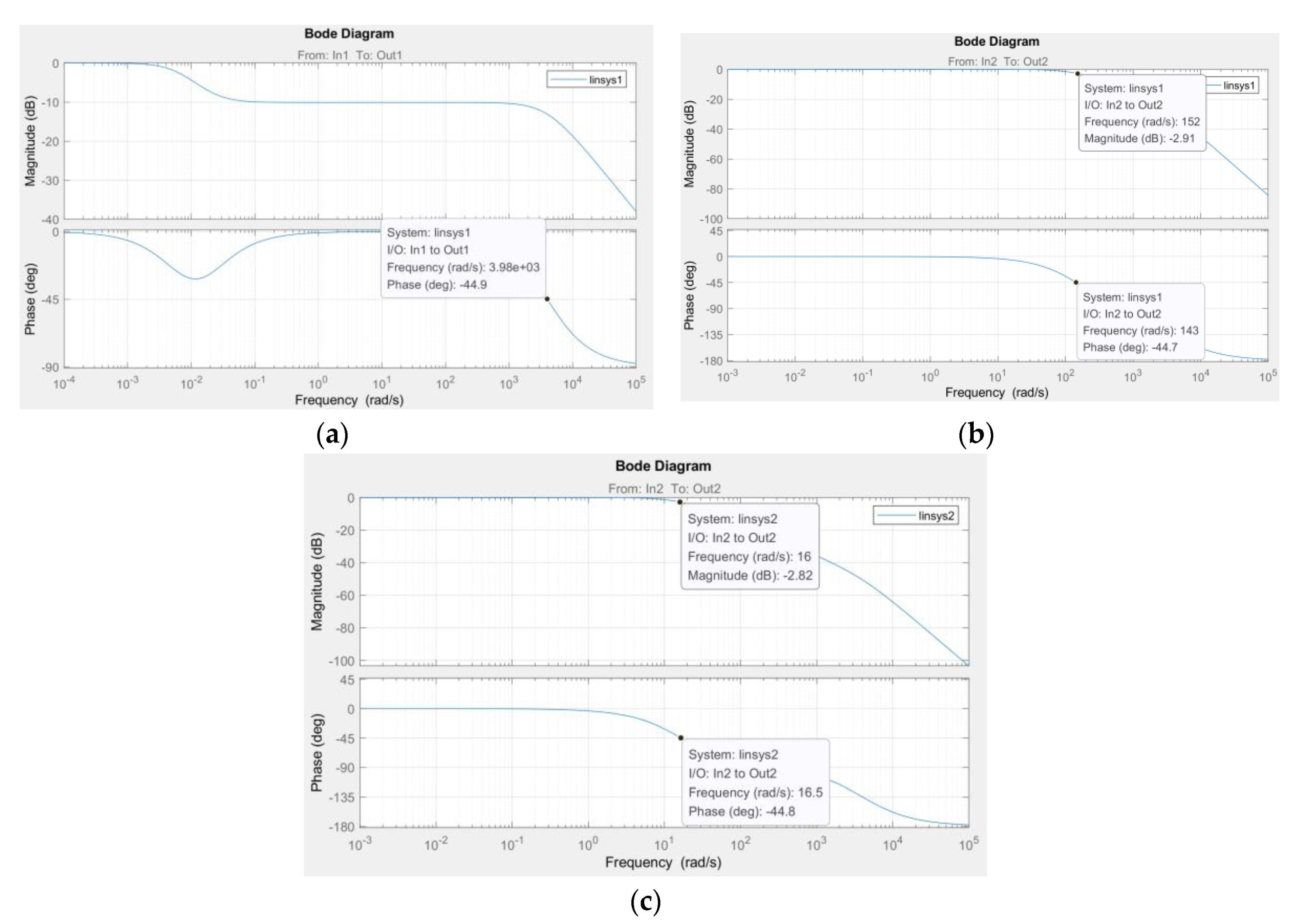
2.5. Digital PI Controller

The analog PI controllers for the position, speed, d-axis and q-axis current control loops are generally expressed as:

$$C(s)=K_p+\frac{K_i}{s}$$

(8)

where $K_p$ and $K_i$ are the parameters of the controller. Equation (8) is digitalized by the backward difference:

$$s=\frac{1-z^{-1}}{T_s}$$

(9)

where $T_s$ is the sampling time. To substitute (9) into (8), we have the general digital PI controller as:

$$C(z)=K_p+\frac{K_i{T}_s}{1-z^{-1}}$$

(10)

An example of the digital PI controller about the q-axis current control loop is shown in Figure 4, where the input ports, fb and cmd, are respectively from the feedback of $i_{qs}$ and the output of the speed PI controller, $i_{qs}^{*}$. $v_{qs}^{*}$ is the output of the q-axis current PI controller. To prevent from the deep saturation of the integral action, an anti-windup action is added to the output of the accumulator (Unit Delay) to limit the maximum accumulated value. The action is especially necessary for the step command input. In addition, saturation is added to the output of the PI controller. The maximum or minimum values of the saturation blocks are depended on the variables to be controlled. For example, the maximum current of the output of the speed controller is set as 3 A. In Figure 5, the $K_{pq}$ and $K_{iq}$ are respectively the proportional and integral control gains, $T_s$ is the sampling time for the q-axis circuit. For current control loops, it is 0.05 ms.

3. The Functional Simulation and Experiments

The parameters of the object used to the functional simulation and practical experiment are shown in

Table 1. The datasheet of proposed linear shaft motor.

Items	Value
Coil resistance (R)	33 Ω
Coil inductance (L)	12 mH
Counter EMF	8.1 V/m/s
Continuous Current	0.6 A rms
Force Constant	24 N/A rms
Continuous Force	15 N
Peak Force	60 N
Magnetic Pitch (North to North)	60 mm
Forcer + Platform of payload	0.5 kg

and

Table 2. The data format of the variables and the parameters of the designed controllers.

Name	Sign Bit	Integer Bit	Fraction Bit	Remark
$K_p$	1	16	15	proportional gain
$K_i$	1	16	15	integral gain
$x$	1	31	0	displacement
$\dot{x}$	1	16	15	speed
$i_d$	1	16	15	d-axis current
$i_q$	1	16	15	q-axis current
$v_d$	1	16	15	d-axis voltage
$v_q$	1	16	15	q-axis voltage
$sin(\theta )$	1	3	28	sine function
$cos(\theta )$	1	3	28	cosine function

illustrates the data format of the variables used to the designed hardware system. The block diagram for the simulation is illustrated in Figure 5. The command is from a square wave with magnitude 1 cm and period 4 s. The position command and position feedback are processed by position controller. By cascade control structure, the output of the position control loop is the command of the speed control loop where the core is the speed controller. The speed controller processes the speed error and its output is proportional to the desired force which could be controlled by the q-axis controller. To the simulated system of vector control, d-axis current command is set as 0 A. The outputs of the two current controllers determine the q- and d-axis voltages, $v_{qs}^{*}$ and $v_{ds}^{*}$, respectively. The coordinate transformations for the phase currents are also illustrated in Figure 5. The units of position, speed and current for demonstration are respectively cm, cm/s and Ampere. Furthermore, speed is got from the position difference operation and is processed by 4th-order moving average. In Figure 5, the block “Gain7” is used to convert the continuous time position into pulse series with gain 10,000 p/cm and “Gain8” is designed to output the digital-type speed. The block “Discrete FIR Filter” runs the 4th-order moving average operation to smooth the ripple of digital speed signal which is got from the position pulse difference operation.

The parameters of the four controllers are listed in

Table 3. The parameters of the proposed controller.

Loop	${\mathit{K}}_{\mathit{p}}$	${\mathit{K}}_{\mathit{i}}$
Position control loop	20	0.3
Speed control loop	10	0.3
d-axis control loop	15	0.3125
q-axis control loop	15	0.3125

, they are verified by the MATLAB/Simulink PID tune APP. With those setting, we have the bode plot of loop gain for current and speed control loops as shown in Figure 6. It shows that the system is stable on both the current and speed control loops. The current loop is with phase margin about 135 degrees and speed control loop has the phase margin about 87 degrees. Furthermore, the current control loop has the closed-loop bandwidth 4020 rad/s (640 Hz) and the closed-loop bandwidth of speed control loop is 152 rad/s (24.2 Hz) with the unload condition or 16.5 rad/s (2.63 Hz) with 4 kg load. Thus, the sampling frequency for current and speed/position are set as 20 kHz and 2 kHz respectively.

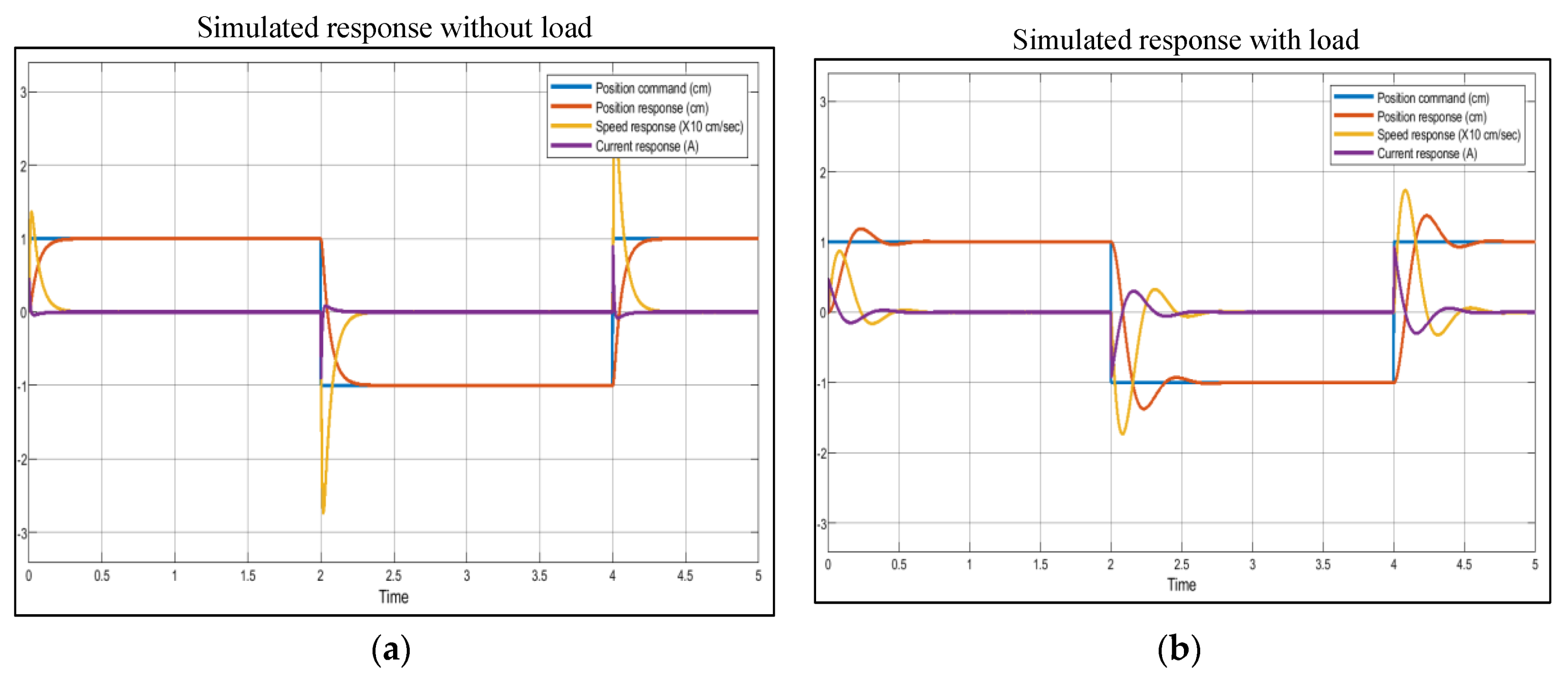
3.1. Simulation Results

The load of the simulation and experiment is from the change of the mass of the forcer. Thus, no load condition is first applied to the simulation. The command is a square wave displacement with magnitude 1 cm and period 4 s. The simulated results are referred to the position command. In Figure 7, we simultaneously demonstrate the position command and the responses of position, speed and q-axis current. The unit of the displacement is cm, the speed is cm/s and the current is ampere (A). According to the vector control strategy, the magnitude of q-axis current is proportional to the generated force. Under the no load condition with the 1 cm displacement command, the maximum speed response is about 26 cm/s and the peak of generated current is about 1 A.

The system with load is assuming a 4 kg object to be put on the forcer, which changes the mechanical system time constant. The simulation results are shown in Figure 7b. For the position response, it is with a 30% overshoot. Since the mass of the forcer is nine times the unload condition, it changes the time constant of the mechanical system. Regarding the speed response, the speed change is not as fast as the unload condition and shows a longer setting time. With respect to the current response, due to the limitation of maximum output of the PI controller, the current is only slightly larger than the no load condition. However, for load condition, the duration of the action of the current is longer than the no load condition.

3.2. Experimental System Setup and Functional Evaluation Results

The experimental hardware system was shown in Figure 1 with the similar position command as the simulation. The evaluation results are shown on the oscilloscope by applying the controlled variables to DAC converter with appropriate ratio. The waveform to the experimental result is shown on the oscilloscope. According to the simulations, the forcer moves forward and backward with the position commands ±1 cm. The 1 cm displacement is equal to 10,000 encoder pulses. A 32-bit counter is designed to feed back the position of the forcer. The speed feedback is calculated from the difference of the displacement counter,

$$v(t)=\frac{dx(t)}{dt}\approx \frac{x(n)-x(n-1)}{T_{ss}}$$

(11)

associated with the following 4th-order moving average operation,

$$H(z)=\frac{1+z^{-1}+z^{-2}+z^{-3}}{4}$$

(12)

where $T_{ss}$ is the sampling time of the speed control loop, which is 0.5 ms. The experimental results are shown in Figure 8. It is noted that all the results are referred to the position command.

The experimental results of no load condition are shown in Figure 8a–c. The position command and the position response are shown in Figure 8a. The square wave has period 4 s and magnitude ±1 cm. Figure 8b shows the speed response and the maximum instantaneous speed is about 26 cm/s. Figure 8c shows the q-axis current response. Since the magnitude of the current is very small, it is a little difficult to be identified as the simulation results.

A 4 kg object is applied to the forcer and fixed on it as the load to change the mass as shown in Figure 1. The control results are shown in Figure 8d–f. Figure 8d shows the waveforms of position command and position response. Figure 8e demonstrates the position command and speed response and Figure 8f shows the q-axis current response referred to the position command. Due to the added load, the speed response is slower than the no load condition. The current response is bigger than the no load condition. Experimental results are quite similar to the simulation results, they prove that the built FPGA-based hardware control system as well as the associated peripherals are efficient.

4. The Trapezoidal Speed Profile Control

Since there are many moving control systems are designed to accept the pulse commands from the motion controller. A trapezoidal speed control profile is thus designed to generate the pulse train command to the linear motor drive system with the constrained displacement and speed considerations. Furthermore, the speed signal of the system is from the incremental encoder with four-time precision and processed by 4th-order moving average. Finally, when the system approaches the destination, it will switch to the position switching control which is used to make the system retain on the desired position with small position error.

4.1. The Generation of Trapezoidal Speed Command Pulse

The trapezoidal speed profile generator to test the system is shown in Figure 9 with the specifications of acceleration 0.6 m/s², constant speed 120 mm/s, deceleration −0.6 m/s² and total displacement 60 mm. Figure 9 demonstrates that in the duration of 0 to 200 ms, the speed starts from 0 and accelerates to 120 mm/s or 12 cm/s. Next, the system keeps at constant speed from 200 ms to 500 ms. After the time instant of 500 ms, it decelerates with the rate −0.6 m/s² and stops at the time instant of 700 ms. The simulated results show that the total displacement is 60 mm which is corresponding to 60,000 encoder pulses while the resolution of incremental encoder pulse is 1 µm. The generated pulses are sent to the position controller of the drive system as the position pulse command.

4.2. The Simulated Results and Problems

The simulation system is shown in Figure 5 and the control results by trapezoidal speed profile command are demonstrated in Figure 10a which includes the position command, the responses of position, speed and q-axis current. Note that the trapezoidal speed profile command of the simulation starts from 0.1 s. As the generated pulse command of Figure 9, Figure 10a demonstrates the speed profile which has the acceleration and deceleration rates the same as the simulation of Figure 9. Furthermore, the speed profile has the maximum speed 12 cm/s and the total duration time about 0.7 s, it is a little longer than the generated profile. Increasing the position control loop gain could reduce the position tracking error, however, it increases the overshoot of the position response. Figure 10b shows the position responses in the vicinity of the final position where the steady-state error is 2 µm. Figure 10c demonstrates the speed response which indicates that the average speed is zero. In speed control loop, speed feedback with pulse difference estimation may result to the steady-state error as the results of Figure 10b. This phenomenon does not relate to the system type but to the method of speed estimation and the sampling frequency. Furthermore, for a fast motion control system, it is difficult to reduce the sampling frequency of the speed control loop.

In this condition, we adopt the switching control which changes the control style as the structure shown in Figure 11. Regarding to the multi-segment sliding mode control system [25], the control structure is designed to be operated at the sliding mode control for all the positioning duration. However, we only adopt the position mode and the system will enter that mode with the decision criterion of (15). A general cascade control structure is switched to the switching mode control structure which bypasses the speed and current control loops. In the study, the speed is from the pulse difference operation followed by 4th-order moving average and the resolution of incremental encoder pulse is 1 µm. In such condition, an encoder pulse difference results to the speed variation,

$$\Delta \dot{x}=\frac{1}{0.0005}(\mathsf{\mu }\mathrm{m}/\mathrm{s})=0.002 (\mathrm{m}/\mathrm{s})$$

(13)

with 4th-order moving average, the possible estimated speed feedback is 0.0005 m/s as shown in Figure 10c. To consider the setting of a position control loop with the proportional gain 70 and position error 2 µm, the position controller output for the speed control loop command will be

$${\dot{x}}^{*}=\pm 2(\mathsf{\mu }\mathrm{m})\ast 70(1/\mathrm{s})=\pm 140(\mathsf{\mu }\mathrm{m}/\mathrm{s})=\pm 0.00014(\mathrm{m}/\mathrm{s})$$

(14)

which does not consider the action of Integral control. It is smaller than the speed feedback as shown in Figure 10c where the estimated speed is ${\dot{x}}_{est}=\pm 0.0005\mathrm{m}/\mathrm{s}$, it is larger than the speed command of Equation (14). This situation can be conquered by adding the Integral action to the position control loop to reduce the steady-state error or increasing the order of the moving average circuit. However, those actions stated above may increase the setting time of position tracking control or result to the time lag of the speed feedback. Thus, the control structure of Figure 11 skips the speed and current control loops while the system approaches to the desired position. The decision machine of Figure 11 is designed as

$$s=\{\begin{array}{c}1,s_1+s_2=2\\ 0,s_1+s_2\ne 2\end{array}$$

(15)

where,

$$s_1(x_e)=\{\begin{array}{c}1,\left|x_e\right|\le 4\mathsf{\mu }\mathrm{m}\\ \mathrm{No}\mathrm{change}\\ 0,\left|x_e\right|\ge 6\mathsf{\mu }\mathrm{m}\end{array}\mathrm{and}{s}_2(\dot{x})=\{\begin{array}{c}1,\left|\dot{x}\right|\le 0.0005\mathrm{m}/\mathrm{s}\\ \mathrm{No}\mathrm{change}\\ 0,\left|\dot{x}\right|>0.0005\mathrm{m}/\mathrm{s}\end{array},$$

and

$$x_e=x^{*}-x$$

is the position tracking error.

The switching control will be activated once the position error and motor speed get into the designed windows, that is, $s=1$ of Equation (15). At that condition, the speed and current controls will be skipped and the output of the position controller directly goes to the inverter input as the voltage command $V_{qs}^{*}$,

$$V_{qs}^{*}=x_e\times K_{pp}\times K$$

(16)

where $K_{pp}$ is the position control gain and the parameter K is set to be

$$K=K_{ps}\times K_{pq}$$

(17)

where $K_{ps}$ and $K_{pq}$ are respectively the speed control and current control gains. It omits the time constant of speed and current control loops and results to a fast response to generate the force to keep the system with a minimum position error. The simulated results of steady-state position responses are shown in Figure 10d where the steady-state position error is $x_e=\pm 1 \mathsf{\mu }\mathrm{m}$.

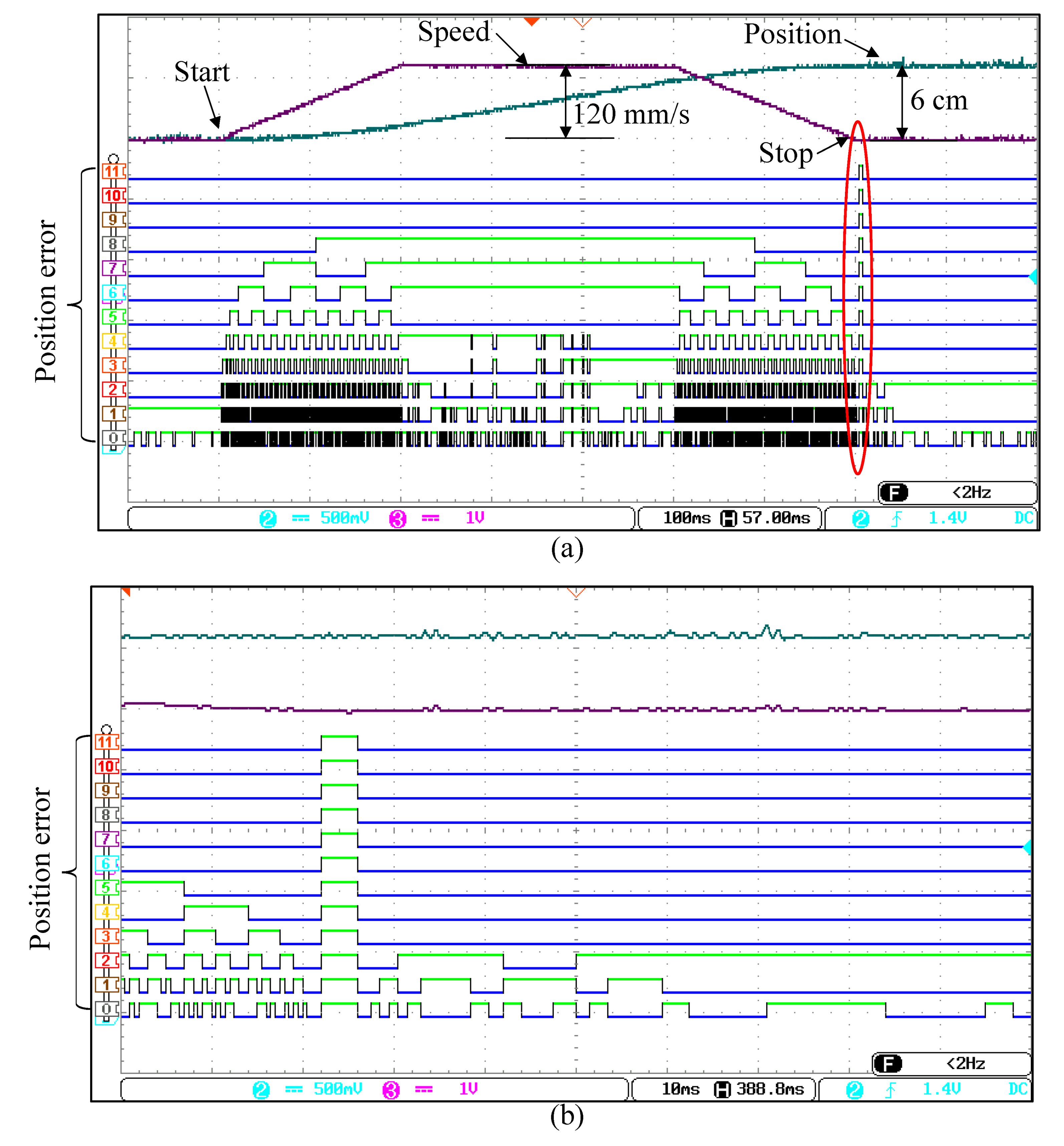
4.3. The Experimental Results with Switching Control

The specifications to the trapezoidal speed profile experiment are with the acceleration 0.6 m/s², constant speed 0.12 m/s, deceleration −0.6 m/s² and total displacement 0.06 m. They are similar to the simulation. The experimental results without the switching control are shown in Figure 12. The position and speed trajectories are from the outputs of DAC converters and the digital position tracking error is from the logical analyzer built in the oscilloscope. Through the logical analyzer, the tracking precision of position response can be clearly demonstrated. In Figure 12a, the time division is 100 ms and the duration from Start to Stop is 700 ms. The speed response demonstrates that the total acceleration period is 200 ms and followed by 300 ms constant speed control period. After that, the system is decelerated and stopped at the destination. It shows that the system responds the same speed profile as simulation. The position offset is between 2 pulses to 5 pulses as shown in the zoom picture of Figure 12b.

Another experiment is run with the switching control and its results are shown in Figure 13a. To clearly demonstrate the steady-state performance with switching control, the zoom picture is shown in Figure 13b. As the results, the steady-state position tracking errors range from −2 pulses to +3 pulses which centers at the desired position.

5. Conclusions

In this study, we have designed a fully digital linear shaft motor drive system in Verilog format and realized on an Altera Cyclone III FPGA. The hardware drive system is successfully tested and verified with step position command. It is also designed to accept the pulse command with trapezoidal velocity profile or S-shape profile. The designed system can also be a part of a complete motion drive system which includes motion control and drive since the resulting hardware code is in the Verilog format. The novelty of paper is shown on the procedure to create the desired control system using the visual block diagram which allows the developers or researchers easily and efficiently to build, simulate, edit, verify and realize their control system from software to hardware.

Because of the cost and the limitation of the memory embedded in the FPGA, the sin/cos look-up table for coordinate transformation and vector control is difficult to have a higher resolution than the stepping motor drive [16] and that causes the problem of accurately positioning on the present structure. The next step of the drive system design for the linear shaft motor by FPGA chip is to solve the above-mentioned problem and adopt some high performance control strategies to the inner current loop or the outer speed loop design. Furthermore, the shaft motor has short time constants on current and speed control loops and controllers could make the bandwidth of the closed-loop broader than the open-loop. Of course, to solve the problem for the noisy feedback current signal is also important for the future work since the magnitude of the current is small.

References

1. Suzuki, A.; Yoshida, T. Position Detection for Shaft-Type Linear Motor by Measurement of Shaft Surface Magnetic Flux. In Proceedings of the International Conference on Electrical Machines and Systems, Tokyo, Japan, 15–18 November 2009. [Google Scholar]
2. Kung, Y.S.; Huang, C.C.; Huang, L.C. FPGA-Based Motion Control IC for Linear Motor Drive X-Y Table Using Adaptive Fuzzy Control. Available online: https://pdfs.semanticscholar.org/ed91/6cc7fb94a8a7c08e06ac6e701168436c5dc5.pdf (accessed on 4 September 2019).
3. Cao, R.; Cheng, M.; Mi, C.; Hua, W.; Wang, X.; Zhao, W. Modeling of a Complementary and Modular Linear Flux-Switching Permanent Magnet Motor for Urban Rail Transit Applications. IEEE Trans. Energy Convers. 2012, 27, 489–497. [Google Scholar] [CrossRef]
4. Hussain, H.A.; Toliyat, H.A. Field Oriented Control of Tubular PM Linear Motor Using Linear Hall Effect Sensors. In Proceedings of the 2016 International Symposium on Power Electronics, Electrical Drives, Automation and Motion, Anacapri, Italy, 22–24 June 2016. [Google Scholar]
5. Xing, F.; Kou, B.; Zhang, L.; Wang, T.; Zhang, C. Analysis and Design of a Maglev Permanent Magnet Synchronous Linear Motor to Reduce Additional Torque in dq Current Control. Energies 2018, 11, 556. [Google Scholar] [CrossRef]
6. Zhang, B.; Qi, R.; Lin, H.; Mwaniki, J. A Model for Analyzing a Five-Phase Fractional-Slot Permanent Magnet Tubular Linear Motor with Modified Winding Function Approach. J. Electr. Comput Eng. 2016, 2016, 1–13. [Google Scholar] [CrossRef] [Green Version]
7. Falkowski, K.; Henzel, M.; Mazurek, P. Mathematical analysis of tubular linear motor. Pomiary Autom. Robot. 2013, 17, 508–512. [Google Scholar]
8. Díaz Pérez, L.C.; Torralba Gracia, M.; Albajez García, J.A.; Yagüe Fabra, J.A. One-Dimensional Control System for a Linear Motor of a Two-Dimensional Nanopositioning Stage Using Commercial Control Hardware. Micromachines 2018, 9, 421. [Google Scholar] [CrossRef] [PubMed]
9. Gao, W.; Chen, X.; Du, H.; Bai, S. Position Tracking Control for Permanent Magnet Linear Motor via Continuous-Time Fast Terminal Sliding Mode Control. J. Control Sci. Eng. 2018, 2018, 1–6. [Google Scholar] [CrossRef] [Green Version]
10. Cao, R.; Cheng, M.; Zhang, B. Speed Control of Complementary and Modular Linear Flux-Switching Permanent-Magnet Motor. IEEE Trans. Ind. Electron. 2015, 62, 4056–4064. [Google Scholar] [CrossRef]
11. Ting, C.S.; Chang, Y.N.; Shi, B.W.; Lieu, J.F. Adaptive backstepping control for permanent magnet linear synchronous motor servo drive. IET Electr. Power Appl. 2015, 9, 265–279. [Google Scholar] [CrossRef]
12. Chaurasiya, B.R.; Patil, M.D.; Shah, D.K.; Kadam, A.V. FPGA Implementation of SVPWM Control Technique for Three Phase Induction Motor Drive Using Fixed Point Realization. In Proceedings of the 2014 International Conference on Circuits, Systems, Communication and Information Technology Applications, Mumbai, India, 4–5 April 2014; pp. 93–98. [Google Scholar]
13. Horvat, R.; Jezernik, K.; Čurkovič, M. An Event-Driven Approach to the Current Control of a BLDC Motor Using FPGA. IEEE Trans. Ind. Electron. 2014, 61, 3719–3726. [Google Scholar] [CrossRef]
14. Ricci, S.; Meacci, V. Simple Torque Control Method for Hybrid Stepper Motors Implemented in FPGA. Electronics 2018, 7, 242. [Google Scholar] [CrossRef]
15. Díaz-Pérez, L.C.; Albajez, J.A.; Torralba, M.; Yagüe-Fabra, J.A. Vector Control Strategy for Halbach Linear Motor Implemented in a Commercial Control Hardware. Electronics 2018, 7, 232. [Google Scholar] [CrossRef]
16. Lai, C.K.; Ciou, J.S.; Tsai, C.C. The Modelling, Simulation and FPGA-Based Implementation for Stepper Motor Wide Range Speed Closed-Loop Drive System Design. Machines 2018, 6, 56. [Google Scholar] [CrossRef]
17. Madrin, F.P.; Hariadi, F.I.; Sasongko, A. Design and Implementation of FPGA-based Control for Linear and Circular Motion Interpolator of PCB CNC-Milling and Drilling Machine. In Proceedings of the 2017 International Symposium on Electronics and Smart Device, Yogyakarta, Indonesia, 17–19 October 2017. [Google Scholar]
18. Zhang, P.; Mills, A.; Zambreno, J.; Jones, P.H. A Software Configurable and Parallelized Coprocessor Architecture for LQR Control. In Proceedings of the 2015 International Conference on ReConFigurable Computing and FPGAs, Mexico City, Mexico, 7–9 December 2015. [Google Scholar]
19. Chen, J.H.; Yau, H.T.; Hung, T.H. Design and implementation of FPGA-based Taguchi-chaos-PSO sun tracking systems. Mechatronics 2015, 25, 55–64. [Google Scholar] [CrossRef]
20. Chiang, H.H.; Hsu, K.C.; Li, I.H. Optimized Adaptive Motion Control Through an SoPC Implementation for Linear Induction Motor Drives. IEEE/ASME Trans. Mechatron. 2015, 20, 348–360. [Google Scholar] [CrossRef]
21. Perng, S.S.; Wu, T.F.; Jiang, M.C.; Li, C.W.; Jiang, Y.R. Based on FPGA Method to Design and Implement for Induction Motors Drive System. J. Comput. 2017, 28, 205–214. [Google Scholar]
22. Nicolas-Apruzzese, J.; Lupon, E.; Busquets-Monge, S.; Conesa, A.; Bordonau, J.; García-Rojas, G. FPGA-Based Controller for a Permanent-Magnet Synchronous Motor Drive Based on a Four-Level Active-Clamped DC-AC Converter. Energies 2018, 11, 2639. [Google Scholar] [CrossRef]
23. Tavana, N.R.; Dinavahi, V. Real-Time FPGA-Based Analytical Space Harmonic Model of Permanent Magnet Machines for Hardware-in-the-Loop Simulation. IEEE Trans. Magn. 2015, 51, 1–9. [Google Scholar] [CrossRef]
24. Diao, L.; Tang, J.; Loh, P.C.; Yin, S.; Wang, L.; Liu, Z. An Efficient DSP–FPGA-Based Implementation of Hybrid PWM for Electric Rail Traction Induction Motor Control. IEEE Trans. Power Electron. 2018, 33, 3276–3288. [Google Scholar] [CrossRef]
25. Shyu, K.K.; Lai, C.K. Incremental Motion Control of Synchronous Reluctance Motor via Multisegment Sliding Mode Control Method. IEEE Trans. Control Syst. Technol. 2002, 10, 169–176. [Google Scholar] [CrossRef]
Figure 1. The experiment setup of linear shaft motor.
Machines 07 00059 g001
Figure 2. The functional block diagram of linear shaft motor drive system.
Machines 07 00059 g002
Figure 3. The block diagram of current vector control.
Machines 07 00059 g003
Figure 4. The structure of PI controller.
Machines 07 00059 g004
Figure 5. The block diagram of the simulation system.
Machines 07 00059 g005
Figure 6. The bode plot of control loops. (a) The current control loop. (b) The speed control loop. (c) The speed control loop with 4 kg load.
Machines 07 00059 g006
Figure 7. The simulation results of square wave position command. (a) No load condition. (b) With 4 kg load condition.
Machines 07 00059 g007
Figure 8. The experimental results of no load and with load.
Machines 07 00059 g008
Figure 9. The simulated result for the Trapezoidal speed profile generator.
Machines 07 00059 g009
Figure 10. The simulation results. (a) The complete position, speed and current responses. (b) The detailed steady-state position response. (c) The detailed steady-state speed response. (d) The detailed position response with switching control.
Machines 07 00059 g010
Figure 11. The modified system control structure.
Machines 07 00059 g011
Figure 12. The experimental results without switching control. (a) The position, speed and position tracking error. (b) Zoom picture of (a).
Machines 07 00059 g012
Figure 13. The experimental results with switching control. (a) The position, speed and position tracking error. (b) Zoom picture of (a).
Machines 07 00059 g013