Article

Non-Rectangular Dynamic Range of the Drive System: A New Approach for the Choice of Motor and Transmission

by
Giancarlo Cusimano
Department of Mechanics, Politecnico di Milano, Via Giuseppe La Masa 1, 20156 Milan, Italy
Machines 2019, 7(3), 54; https://doi.org/10.3390/machines7030054
Submission received: 9 July 2019 / Revised: 1 August 2019 / Accepted: 4 August 2019 / Published: 29 August 2019

Abstract

:
This paper deals with the choice of the motor-transmission couple to drive a joint in the frequent case in which the limit curve of the dynamic operating range of the drive system depends on the motor speed. The paper considers a given drive system and proposes a method that resorts to a succession of instant analyses during the reference task: for a transmission with no energy dissipation the result, if it exists, is a range of transmission ratios that can be coupled with the given motor in order to perform the reference task. The extension of the method to a real transmission is a diagram that correlates the transmission ratio and the direct and inverse efficiency of the reducer and that offers the designer an overview of the transmissions that can be coupled with the given motor to perform the reference task.

1. Introduction

In mechatronic applications, the electrical drive system and the transmission suitable to drive a joint must be chosen in consideration of each other. Many characteristics regarding both components affect the selection of this couple. In particular, the continuous duty operating range of the motor, related to its thermal problem, and the dynamic operating range of the drive system, related to the torque peak of the motor, are generally decisive, because they impose strict constraints on this choice. Both issues must be taken into account in the design. Often, the two operating ranges are considered rectangular and this simple geometry appreciably helps the computing process.
Many papers dealt with the simultaneous choice of drive system and reducer. Some quite recent works [1,2,3,4] directly tackled the automatic optimization of this choice, taking into account the above-mentioned constraints. If the optimization is multi-objective, it permits not only the limitation of one objective function, for instance the cost, but also the improvement of the machine performance, for example of its control errors. The mutual influence of the different power trains is also taken into account in multi-D.o.F. machines. In general, these papers considered rectangular operating ranges of the drive systems. In [5] the optimization is carried out by the designer by comparing different diagrams.
Conversely, the more classical selection procedure is composed of two subsequent steps, as is indicated by [6]:
-
The feasibility analysis allows the designer to exclude all the drive system-transmission couples that are not able to drive the given load from the point of view of their operating ranges, i.e., of their torque and speed characteristics. In this phase, one (or more than one) reference task is taken into consideration, assuming that the machine executes it perfectly, i.e., with no control error. It is clear that a drive system-reducer couple can be excluded because of either the thermal problem or the torque peak problem. The feasibility analysis permits the designer to rapidly limit the number of admissible motor-transmission couples and, if convenient, to apply his experience to them to further restrict this set, in order to proceed with the optimization phase.
-
Then, the optimization phase allows the designer to find the motor-transmission pair that best meets some additional criteria (minimum cost, weight, volume etc.).
Many authors dealt with the first phase and devised different methods to individuate the admissible motor-transmission couples. They assumed that the drive system operating ranges are rectangular. Sometimes they only considered the torque peak problem of the motor [7,8,9], sometimes only the thermal problem [10,11], sometimes both of them [6,12,13]. The number of parameters, characterizing motor and transmission, taken into consideration increased more and more over time.
Some authors [14,15] took into account either continuous duty or dynamic operating ranges that are non-rectangular, as is necessary for many drive systems.
In [15] Cusimano analyzed the issues arising when the method explained in [8,9] is applied to a drive system whose dynamic operating range is non-rectangular: it does not always allow the designer either to determine if a drive system is admissible or, when it is admissible, to completely determine the range of transmission ratios it can be matched with.
This paper still deals with the feasibility analysis when the dynamic operating range of the drive system is non-rectangular. First of all, it desires to eliminate the uncertainties present in [15] by resorting to a new approach. This is based on taking into account a given drive system and carrying out a succession of instant analyses during the reference task: at each time t the method proposed permits the designer to find, if it exists, a range [ τ m i n ( t ) ,   τ m a x ( t ) ] of transmission ratios that allows the motor to drive the load at that time. The result of all these analyses is a range [ τ m i n * ,   τ m a x * ] of transmission ratios, if it exists, that allows the motor to drive the load during the complete reference task.
Furthermore, this paper desires to take into account not only the transmission ratio, but also the efficiencies of the reducer. It achieves this purpose by extending the above-mentioned procedure to the case of a transmission dissipating energy. The calculation is automated, so that the final result is a diagram that offers the designer an overview of which reducers, characterized by their transmission ratio and efficiencies, can be coupled with the given drive system in order to perform the reference task. This diagram is a generalization of that obtained, by another method, in [9] for a drive system with a rectangular dynamic operating range.
More specifically, Section 2 presents the parameters characterizing motor and transmission. Section 3 assigns the specifications, which refer to the load, and establishes the inequalities due to the dynamic operating range of the motor. Section 4 illustrates a classical approach, while Section 5 explains the reasons and the outlines of the new approach. Section 6 provides the equation of the limit curve of the dynamic operating range. Section 7 concisely explains the procedure of the new approach. In Section 8, the effects of the efficiency and inertia of the reducer are introduced. Section 9 presents a case study. Finally, Section 10 sets out the conclusions.

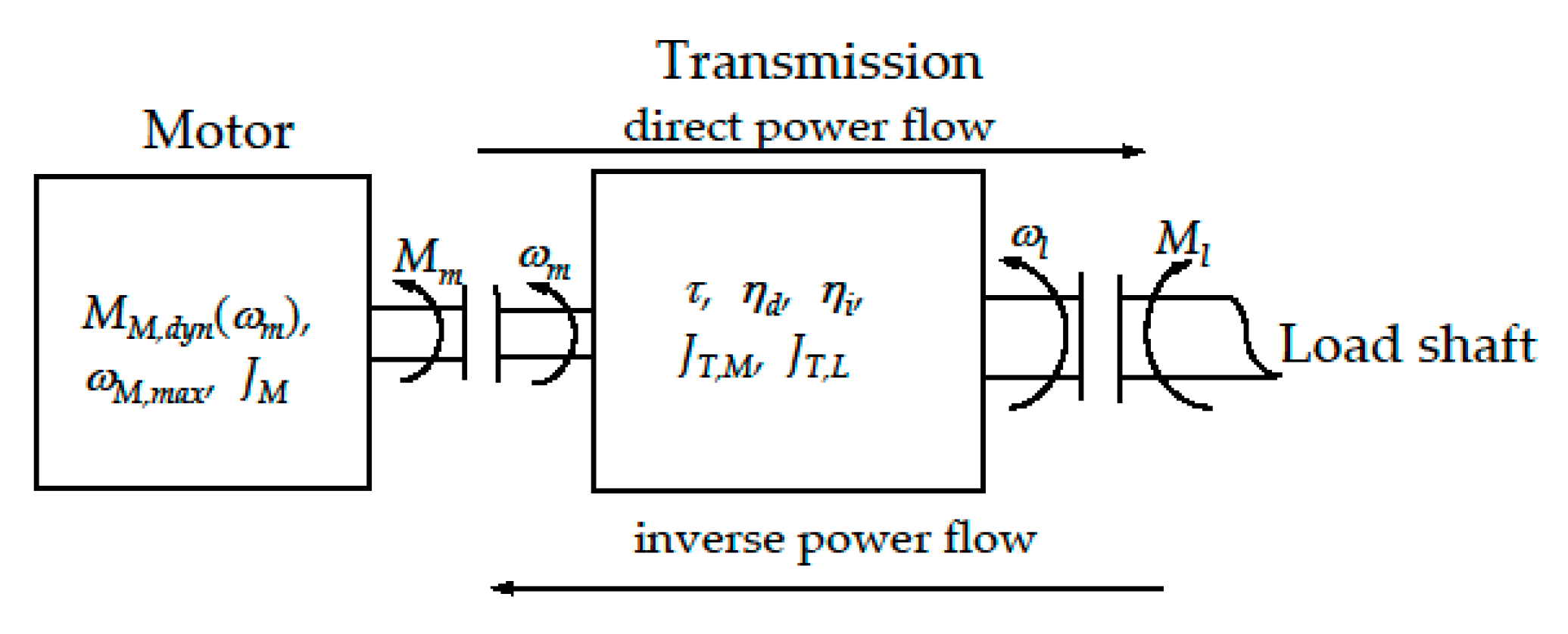
2. Drive System and Transmission Characterization

In Figure 1 an electrical motor moves a load through a reducer. In this machine, only one degree of freedom is taken into account for the choice of motor and reducer, because the influence of other possible degrees of freedom is expressed by the load torque M l acting on the joint, which is a known function of time.
A permanent magnet brushless servo-motor is taken into consideration. Its unknown moment of inertia is J M . The current motor torque is denoted by M m and its speed by ω m . The motor operating ranges are shown in Figure 2.
The continuous duty range, whose limit torque is M M , S 1 , is related to the thermal problem of the motor and is not considered in this work. However, it is clear that motor and transmission must be chosen so as to respect also this operating range.
The dynamic operating range of the drive system is bounded by the maximum speed ω M , m a x and by a torque M M , d y n , which in general depends on the motor speed
M M , d y n = M M , d y n ( ω m )
Torque M M , d y n is mainly determined by the electronic drive feeding the motor and is the maximum torque that the motor can exert at each speed. In the limit curve of the dynamic operating range there are two characteristic points: N 1 , whose coordinates are ω M , 1 and M M , d y n , 1 , and N 2 , whose speed and torque are ω M , m a x and M M , d y n , 2 , respectively. M M , d y n is constant and equal to M M , d y n , 1 when the speed is lesser than ω M , 1 Conversely, to the right of N 1 , M M , d y n decreases as far as speed ω M , m a x . The two arcs are due to two saturation phenomena: whereas the horizontal segment, whose ordinate is M M , d y n , 1 , is due to the maximum current that the electronic converter can supply, the descending arc is due to the simultaneous saturation of the voltage applied to the motor. In this condition, the electronic driver is often subject to the flux-weakening technique [16] that permits a broadening of the dynamic operating range, even though with a decreasing value of torque M M , d y n ( ω m ) . The descending arc presents a regular maximum at ω M , 1 .
Therefore, in general, the limit curve s of the dynamic operating range of the drive system is composed of:
-
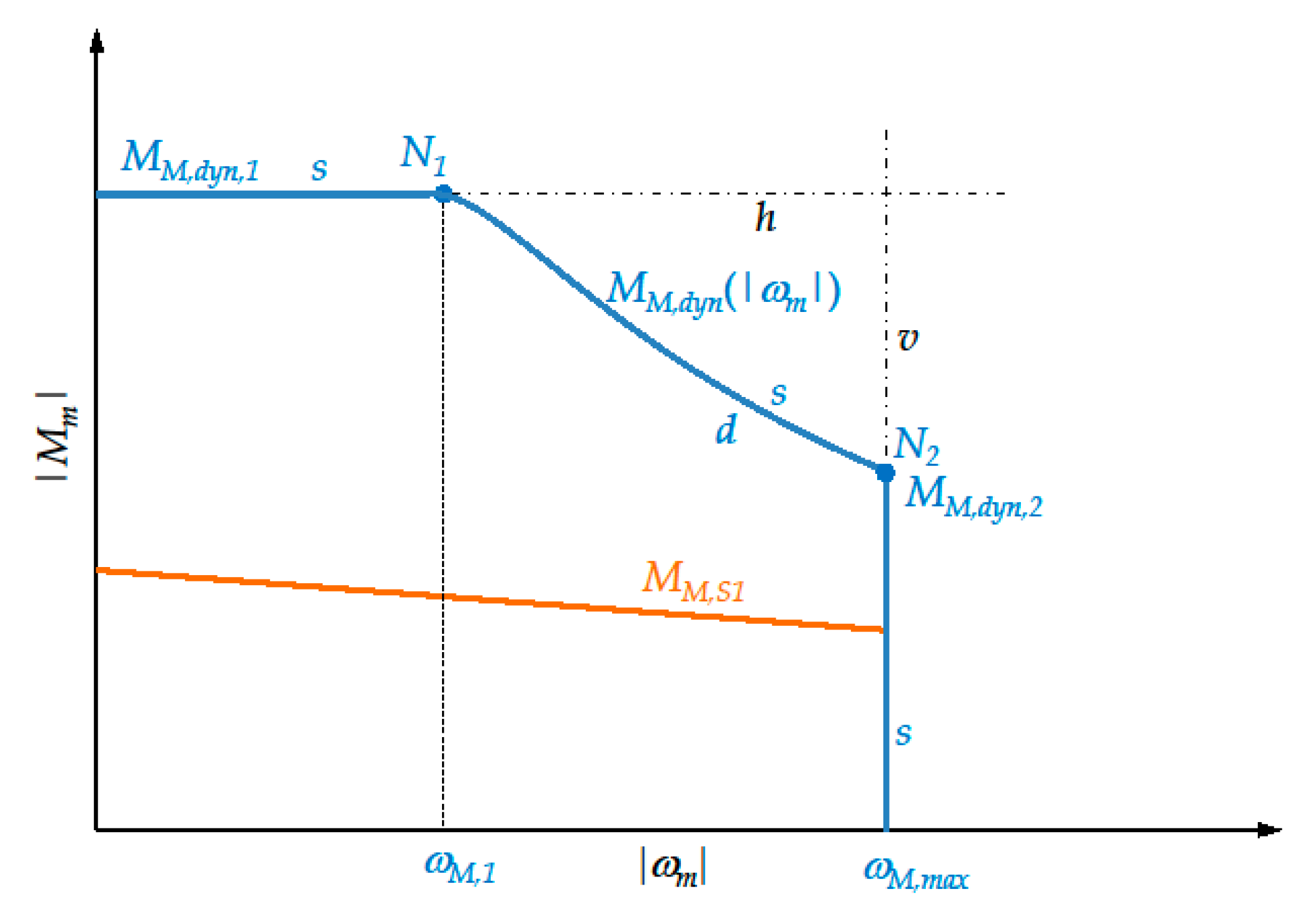
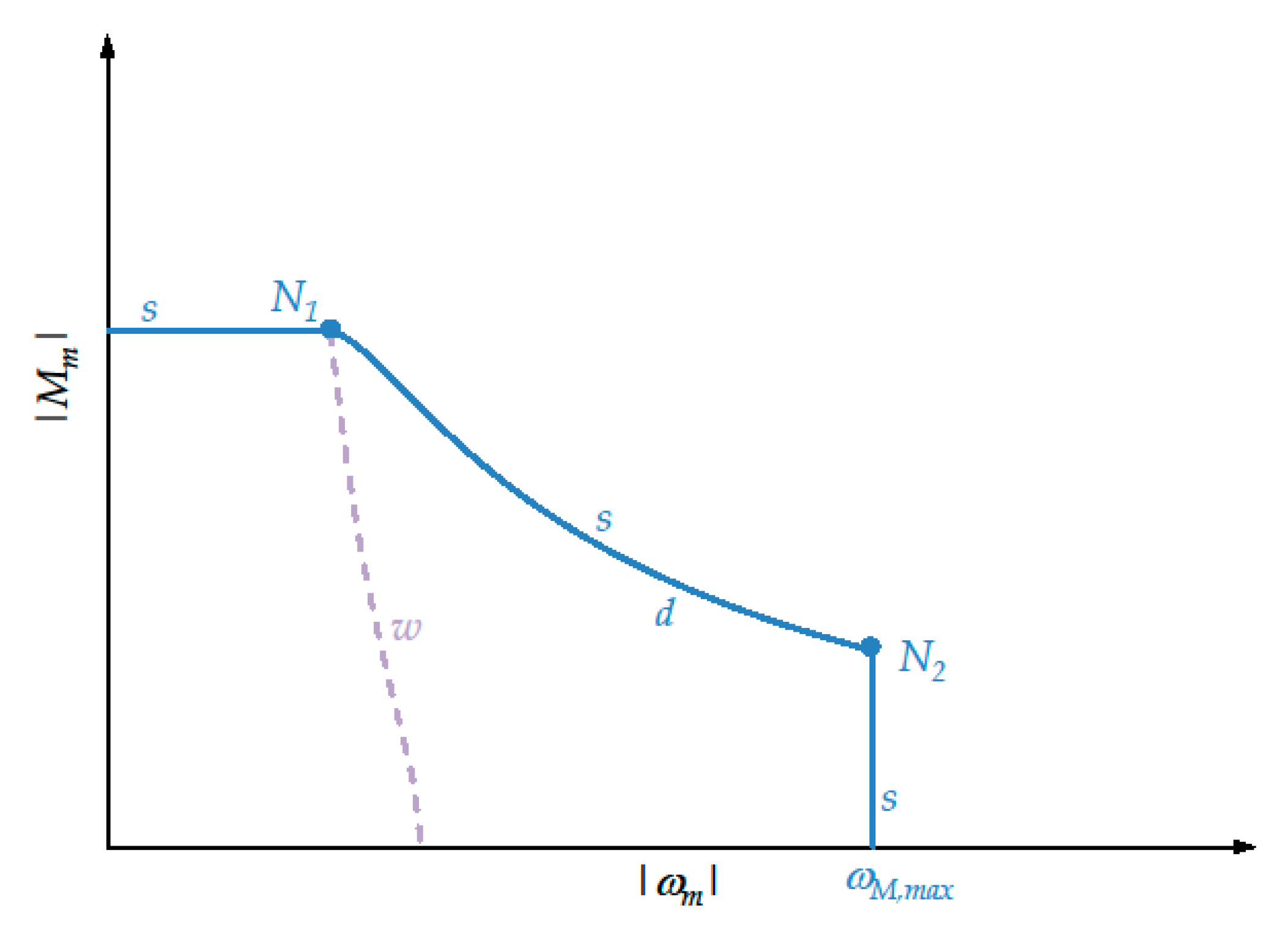
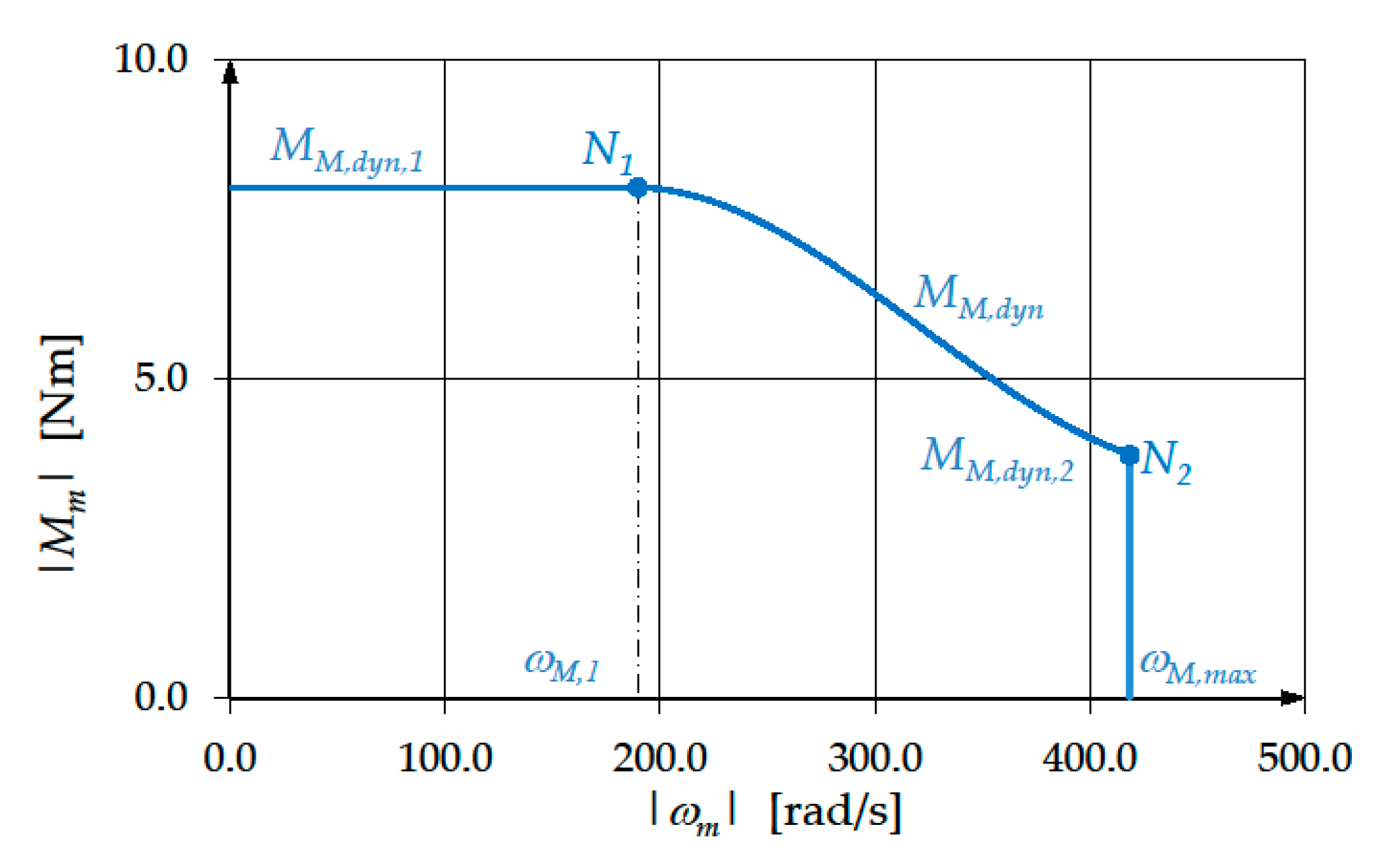
A horizontal segment belonging to the straight-line h, with a constant torque equal to M M , d y n , 1 , due to current saturation;
-
A descending arc d (arc N 1 N 2 ), which is the limit curve of the dynamic operating range of the drive system corresponding to the saturation of both current and voltage;
-
A vertical segment belonging to the straight-line v, with a constant speed equal to ω M , m a x , which is electronically fixed by the drive system.
A reducer is interposed between motor and load. Its transmission ratio τ is the ratio between load speed ω l and motor speed ω m
τ = ω l ω m
For the sake of simplicity and without loss of generality, this paper assumes that the transmission ratio τ is positive.
At the beginning, the hypothesis is that the transmission has negligible inertia and no energy dissipation. This assumption is justified by these considerations:
-
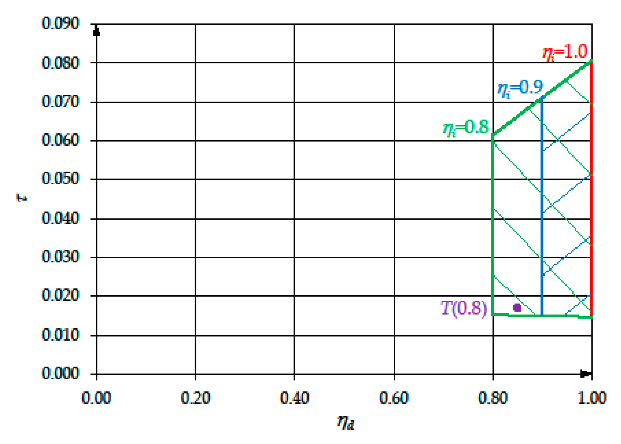
The transmission efficiencies are often quite high and the introduction of a certain safety margin maintains the validity of the choices made with reference to the ideal case.
-
The moments of inertia of the transmission, J T , M on motor side and J T , L on load side, are often negligible compared to the moments of inertia of motor and load, respectively.
Nevertheless, above all, these initial assumptions are due to the fact that this paper desires to explain the method proposed in its simplest form, without introducing aspects that would render the explanation superfluously complex. However, afterwards, Section 8 will show that it is not difficult to extend the results obtained to the case of a real transmission.

3. Task Specifications and Inequalities due to the Dynamic Operating Range

For the choice of the motor from the point of view of its dynamic operating range, a single reference task, which is particularly demanding because of high motor torques and speeds, is here considered.
As regards the specifications, during the reference task the angular speed ω l ( t ) of the joint is considered a known function of time, together with its acceleration α l ( t ) . The load torque M l ( t ) applied to the joint is also a known function of time. It takes into account the contribution of the resistant and inertial forces acting on the machine.
In general, during the machine running the motor torque M m is a non-single-valued function of the motor speed ω m
M m = M m ( ω m )
It is clear that, because of the motor dynamic operating range, the following set of inequalities must be satisfied at any instant t
{ | M m ( | ω m | ) | M M , d y n ( | ω m | ) | ω m | ω M , m a x
This means that the curve expressed by Equation (3), mapped in the first quadrant, must lie inside the dynamic operating range of the drive system. Hence, from the point of view of its dynamic operating range, the drive system must satisfy inequalities (4).

4. Classical Approach

In the case of a rectangular dynamic operating range, the approach explained in [8,9] resorts to a diagram with suitable coordinates (Figure 3) in which:
-
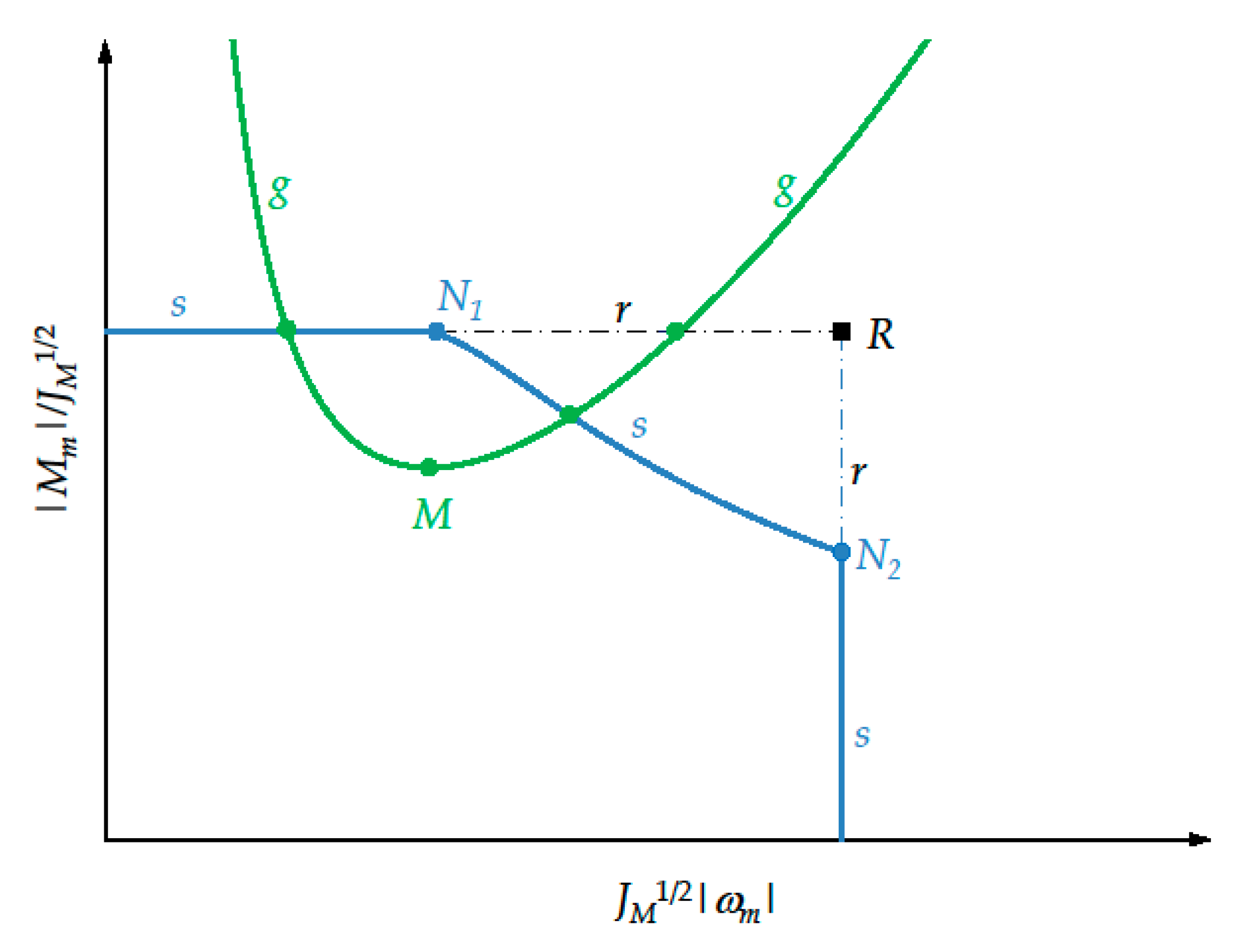
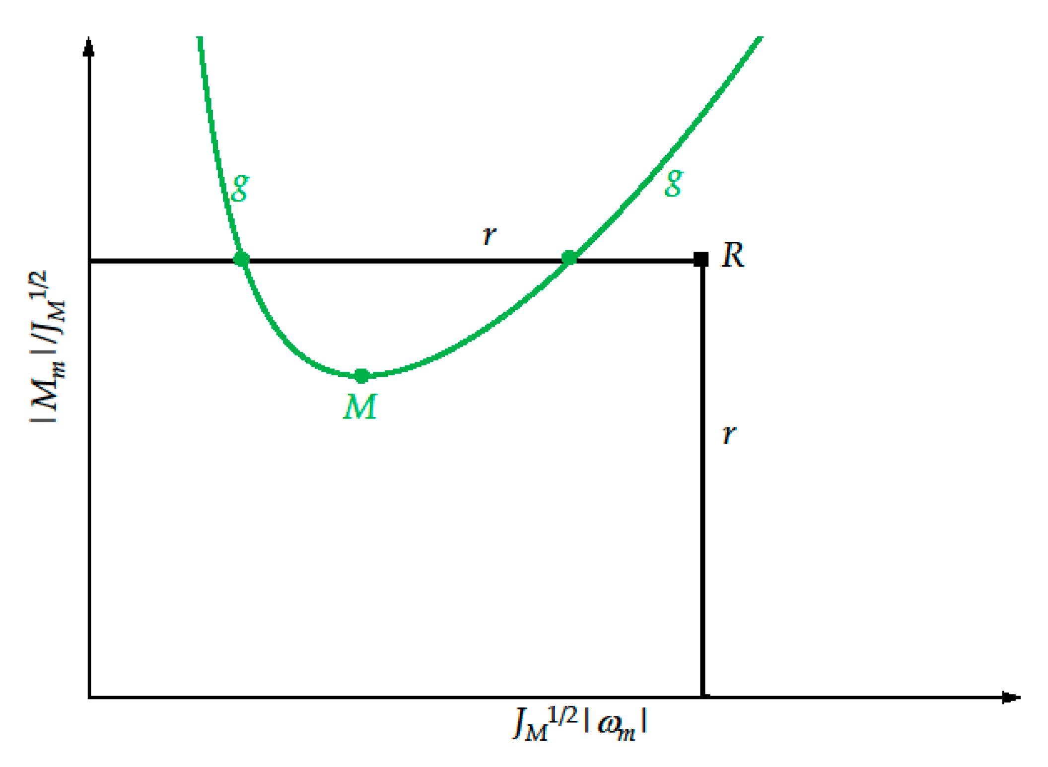
A global load torque curve g is taken into consideration, i.e., a curve that depends on the global reference task; this curve depends on the load speed only through its maximum value ω l , m a x , where
ω l , m a x = max t [ | ω l ( t ) | ]
or is a specification independent of the reference task and greater than the value given by Equation (5).
-
Each drive system is represented by a corresponding point, i.e., the vertex R of the rectangular dynamic operating range, whose limit curve is denoted by r.
This diagram permits a comprehensive and simultaneous view of all the drive systems. Some of them must be excluded, whereas the admissible motors are able to drive the load according to the reference task only if they are coupled with a reducer whose transmission ratio lies in a defined range [ τ m i n * ,   τ m a x * ] . This range is characteristic of each motor and can be easily found. This means that motor and transmission must be chosen in mutual correlation.
If the dynamic operating range of the drive system is non-rectangular, a similar approach can still be adopted [15], but with some limitations. A similar diagram (Figure 4) shows the representation of:
-
The same global load torque curve g as before.
-
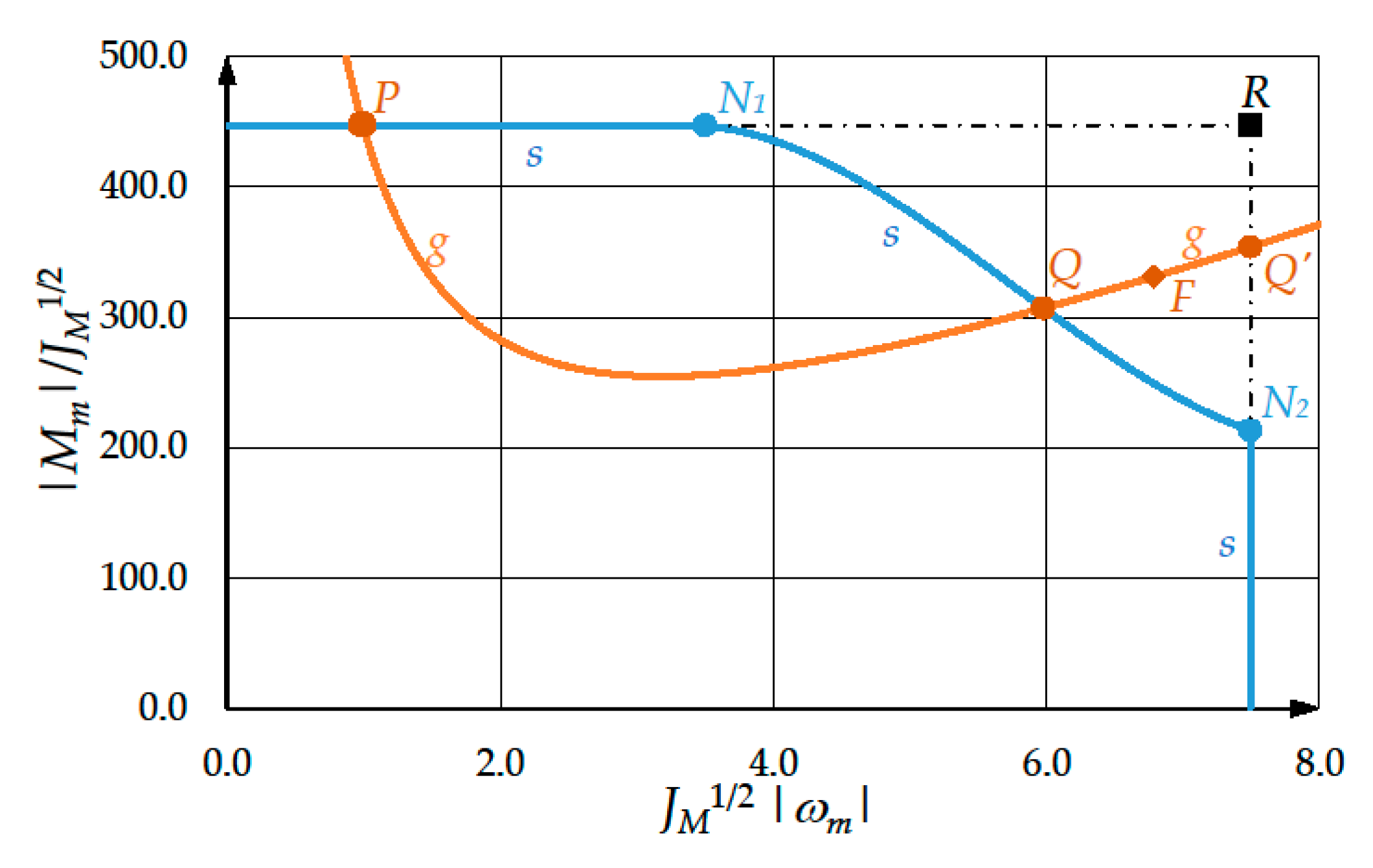
Each drive system not only by means of the corresponding non-rectangular dynamic operating range, whose limit curve is denoted by s, but also by means of the corresponding rectangular operating range, denoted by r. Its vertex is denoted by R.
The advantage of this method is that for some drive systems the solution is complete because
(1)
The drive system must surely be excluded;
(2)
The transmission ratio range [ τ m i n * ,   τ m a x * ] in correspondence to which the motor can be adopted is perfectly defined.
Nevertheless, the disadvantage is that there are other drive systems for which the method does not allow the designer:
(1)
To ascertain if they are admissible or not;
(2)
To completely determine the corresponding transmission ratio range for motors whose admissibility is already known.
In order to avoid these uncertainties, in this paper a different method is adopted. It works by taking into account a given motor at a time and finding the corresponding transmission ratio range [ τ m i n * ,   τ m a x * ] by means of a succession of instant analyses of the global machine.

5. The New Approach

5.1. Outlines of the New Approach

An ideal reducer with negligible inertia and no energy dissipation in now taken into account; it is only characterized by its transmission ratio τ, which is unknown. The motor quantities ω m ( t ) and M m ( t ) , subject to inequalities (4), can be easily obtained by means of the load quantities ω l ( t ) , α l ( t ) and M l ( t ) and the transmission ratio τ. Taking into account Equation (2), the absolute value of the motor speed is equal to
| ω m ( t ) | = | ω l ( t ) | τ
At each instant, for each motor and transmission the rotation equilibrium at the joint is expressed by the relation
M m ( t ) τ = J M τ 2 α l ( t ) + M l ( t )
Multiplying all the terms by τ, Equation (7) gives
M m ( t ) = J M τ α l ( t ) + τ M l ( t )
The absolute value of the motor torque is equal to
| M m ( t ) | = | J M τ α l ( t ) + τ M l ( t ) |
At a given instant, the absolute value of the motor torque can be considered as a function of the transmission ratio τ, with t as a parameter:
| M m ( τ ;   t ) | = | J M τ α l ( t ) + τ M l ( t ) |
Substituting for τ from Equation (6) into Equation (10) and taking into account that ω l ( t ) is known at the instant considered, the absolute value of the motor torque becomes a function of the absolute value | ω m | of the motor speed, with t as a parameter
| M m ( | ω m | ;   t ) | = | J M α l ( t ) | ω l ( t ) | | ω m | + M l ( t )   | ω l ( t ) | 1 | ω m | |
The corresponding curve is called instantaneous load torque curve and denoted by l.
In the new approach, at each instant, the instantaneous load torque curve l is compared with the limit curve s of the dynamic operating range in the | ω m | | M m | plane in order to check if inequalities (4) are met, as is explained below.
The reference task can be regarded as a succession of close instants, which are taken into consideration one after another. If at the preceding instants the drive system has not been excluded yet, the new instant t is considered, with the corresponding values of ω l ( t ) , α l ( t ) and M l ( t ) . In the | ω m | | M m | plane, curves l and s can have none or two intersection points, or can be tangent (Figure 5).
If the intersection points are two (curve l 2 ), they have different abscissas, denoted by ω m , m i n ( t ) for the intersection point to the left and ω m , m a x ( t ) for that to the right.
It is noteworthy that the drive system is able to exert the torque required by the load only in the speed range [ ω m , m i n ( t ) ,   ω m , m a x ( t ) ] in which the instantaneous load torque curve l lies inside the dynamic operating range of the drive system. This speed range corresponds to a range [ τ m i n ( t ) ,   τ m a x ( t ) ] of transmission ratios that permit the motor to drive the load at the instant considered. In fact, bearing in mind Equation (2), the two extreme transmission ratios are given by
τ m i n ( t ) = | ω l ( t ) | ω m , m a x ( t )
τ m a x ( t ) = | ω l ( t ) | ω m , m i n ( t )
Since the maximum possible value of ω m , m a x ( t ) is ω M , m a x , in any case the following inequality is met
τ m i n ( t ) | ω l ( t ) | ω M , m a x
If there is no intersection point between the two curves (curve l 0 ), there is no value of the transmission ratio that makes the motor able to drive the load at the instant considered, and the motor must be definitively excluded. Furthermore, if the two curves are tangent (curve l 1 ), it is precautionary to exclude the motor.
In short, a motor is said admissible at instant t if there is a range of transmission ratios it can be coupled with it in order to move the load at that instant. A single instant in which the drive system is not admissible is sufficient to exclude it definitively.
Vice versa, it is noteworthy that if the drive system is admissible at all the instants it is not yet sure that it is able to drive the load during the complete reference task. In fact, if, after having repeated the above-described analysis at all the subsequent instants, the motor has never been excluded, the result is a succession of valid transmission ratio ranges [ τ m i n ( t ) ,   τ m a x ( t ) ] . The drive system can be considered definitively admissible only if these transmission ratio ranges have an intersection common to all, i.e., if they have a common interval [ τ m i n * ,   τ m a x * ] : in this case the motor is able to drive the load during the reference task if it is coupled with an ideal reducer whose transmission ratio lies in this interval. Otherwise, the motor must be excluded.
These conditions can be checked by considering the maximum τ m i n * of the minimum transmission ratios τ m i n ( t ) over time
τ m i n * = max t [ τ m i n ( t ) ]
and the minimum τ m a x * of the maximum transmission ratios τ m a x ( t ) over time
τ m a x * = min t [ τ m a x ( t ) ]
If τ m i n * is lesser than τ m a x * , the range [ τ m i n * ,   τ m a x * ] is the intersection sought among all the ranges [ τ m i n ( t ) ,   τ m a x ( t ) ] . Conversely, if τ m i n * is greater than τ m a x * , the motor must obviously be excluded.

5.2. New Approach for a Non-Rectangular Dynamic Operating Range

For a rectangular dynamic operating range it is simple to show that τ m a x * does not depend on the load speed ω l ( t ) in any way, whereas τ m i n * can depend only on the maximum load speed ω l , m a x . Therefore, a succession of instant analyses is unnecessary and in this case a global load torque curve g can be used; it depends on the load speed only through its maximum value ω l , m a x .
Conversely, if the given motor has a non-rectangular dynamic operating range (Figure 6), the treatment is more complex because there are particular cases that require the computation of the possible intersections between the instantaneous load torque curve l and the descending arc d. In particular:
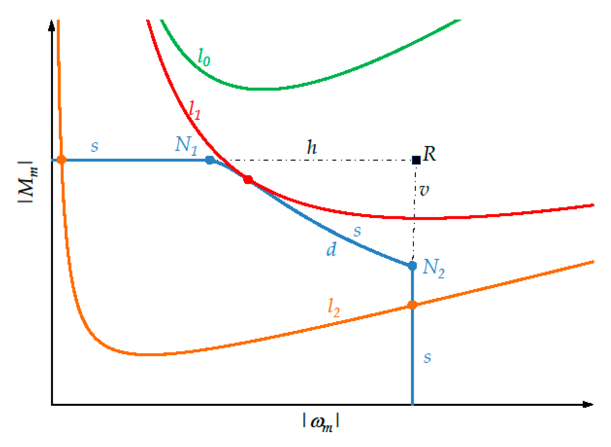
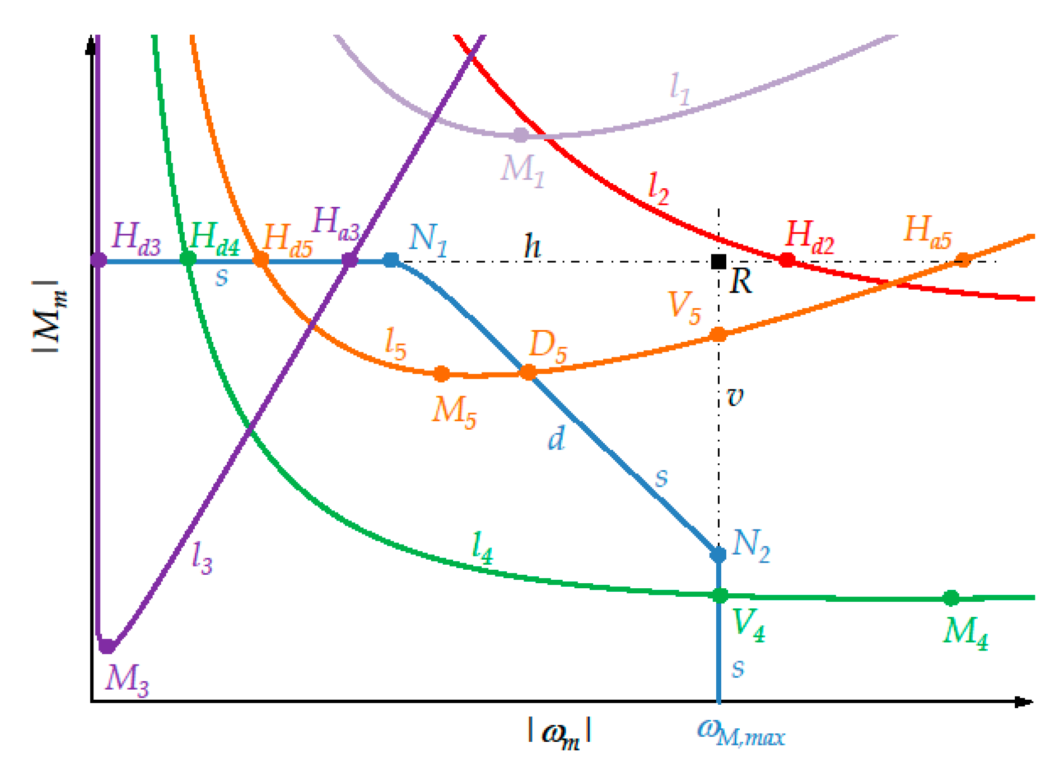
  • Curve l can intersect the curvilinear triangle R N 1 N 2 , but not the limit curve s of the dynamic operating range (curve l 1 ): in this case the drive system must be excluded.
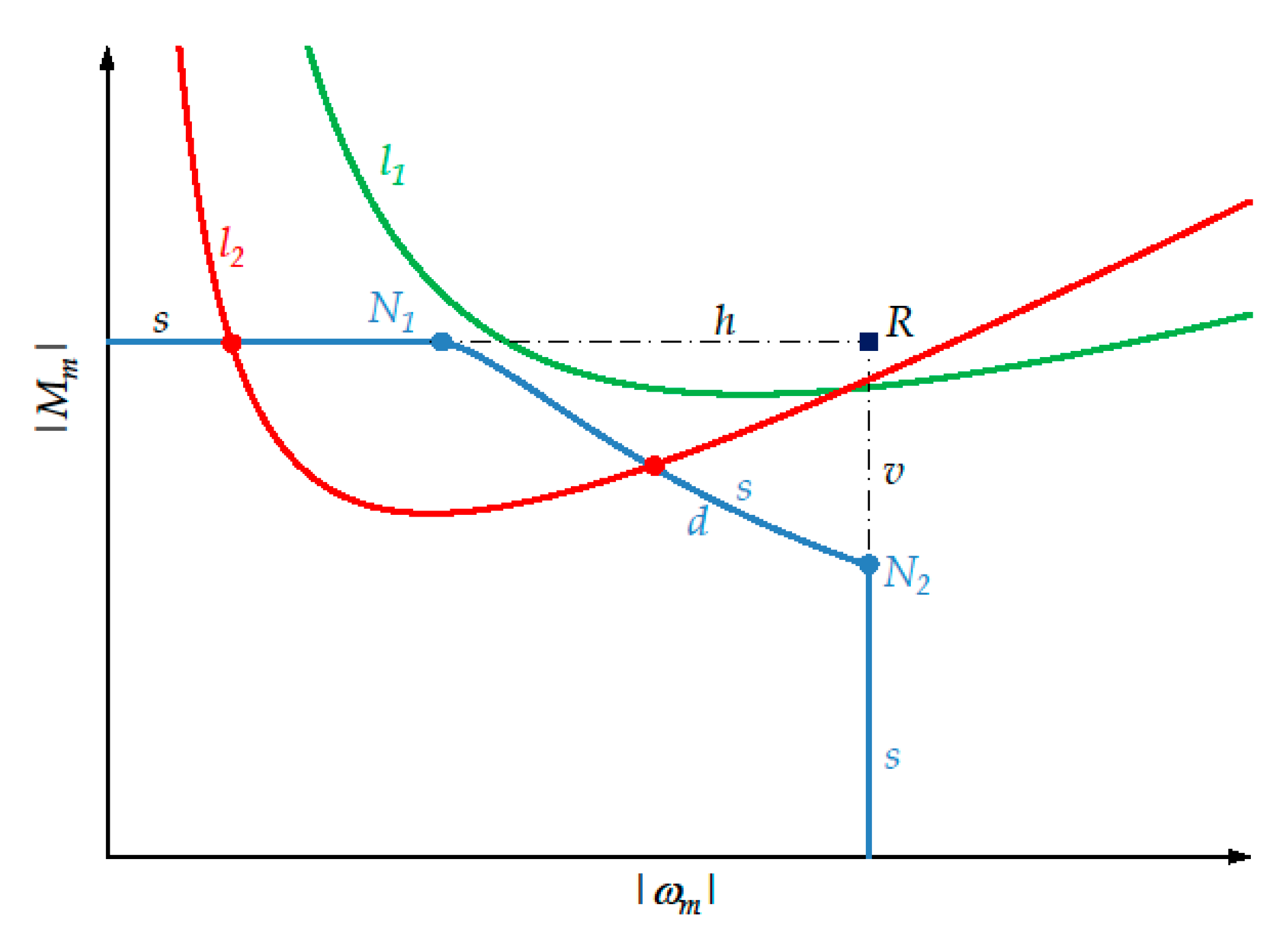
  • Curve l can intersect the limit curve of the dynamic operating range in correspondence to arc d (curve l 2 ).
The transmission ratios corresponding to the intersections between curve l and arc d can be found by means of equation
| M M , d y n [ | ω l ( t ) | τ ] | = | J M τ α l ( t ) + M l ( t ) τ |
They do depend on ω l ( t ) : this is why referring only to ω l , m a x is not possible, but a succession of instant analyses must be carried out for a non-rectangular dynamic operating range. In order to find, numerically, the possible intersections between curve l and arc d an analytic expression of the latter is required, as is shown in the next section.

6. Limit Curve of a Non-Rectangular Dynamic Operating Range

Normally, a brushless motor [16] is a three-phase motor, but its control theory is based on the transformation into an equivalent two-phase motor. The permanent magnets are in the rotor, where a set of axes d–q is taken into consideration. The direct axis d has the direction of the magnetic flux Ψ of the permanent magnets, whereas the quadrature axis q is orthogonal to d. In the two-phase motor, two different currents flow in the two stator windings, and they can be represented by a phasor, which is denoted by I ¯ . At each instant, i.e., at each rotor position, the phasor I ¯ can be projected onto the two axes d and q and its two components are the direct current I d and the quadrature current I q , respectively. Motor torque M m only depends on the quadrature current I q and in linear conditions is proportional to it.

6.1. Limit Curve Equation in Ideal Conditions

The hypotheses are now that there is linearity between motor torque M m and quadrature current I q up to the maximum current and that the winding resistances are constant. When the flux-weakening technique is not applied, the dynamic operating range is limited to the right by a descending arc (arc w in Figure 7); its expression is obtained in Appendix A. Conversely, when the flux-weakening technique is applied the expression of M M , d y n ( | ω m | ) is obtained in Appendix B and is equal to
M M , d y n ( | ω m | ) = R p h [ V m a x 2 K E 2 ω m 2 Z 2 I m a x 2 ] 2 | ω m | Z 2 + n | ω m | L s 4 Z 2 I m a x 2 K E 2 ω m 2 [ V m a x 2 K E 2 ω m 2 Z 2 I m a x 2 ] 2 2 | ω m | Z 2
where
Z 2 = R p h 2 + n   2 ω m 2 L s 2
and
I m a x = 3 I m a x , c o n v
The parameters n, R p h , L s , V m a x , K E and I m a x , c o n v are directly found in the motor and drive system catalog and Equation (18) is valid in the speed range [ ω M , 1 ,   ω M , m a x ] , where
ω M , 1 = R p h I m a x K E n 2 L s 2 I m a x 2 + K E 2 [ 1 + ( V m a x 2 R p h 2 I m a x 2 ) ( n 2 L s 2 I m a x 2 + K E 2 ) R p h 2 I m a x 2 K E 2 1 ]
In correspondence to ω M , 1 the curve shows a regular maximum (Figure 7), then is descending, with possible concavity changes. It is electronically interrupted at speed ω M , m a x .
Appendix B also shows that, substituting for | ω m | from Equation (6) into Equation (18), M M , d y n becomes a function of the transmission ratio τ, with t as a parameter
M M , d y n ( τ ;   t ) = τ { [ τ 2 V m a x 2 K E 2 ω l 2 ( t ) ] [ τ 2 R p h 2 + n 2 ω l 2 ( t ) L s 2 ] I m a x 2 } 2 | ω l ( t ) | [ τ 2 R p h + n 2 ω l 2 ( t ) L s 2 R p h ] + n | ω l ( t ) | L s R p h 4 [ τ 2 R p h 2 + n 2 ω l 2 ( t ) L s 2 ] I m a x 2 K E 2 ω l 2 ( t ) { [ τ 2 V m a x 2 K E 2 ω l 2 ( t ) ] [ τ 2 R p h 2 + n 2 ω l 2 ( t ) L s 2 ] I m a x 2 } 2 2 | ω l ( t ) | [ τ 2 R p h + n 2 ω l 2 ( t ) L s 2 R p h ]
More concisely, M M , d y n ( τ ;   t ) can be written as
M M , d y n ( τ ;   t ) = k 1 τ 3 + k 2 τ + k 3 τ 4 + k 4 τ 2 + k 5 k 6 τ 2 + k 7
where, after having defined
{ V 1 2 = V m a x 2 R p h 2 I m a x 2 V 2 2 = ( n L s | ω l ( t ) | ) 2 I m a x 2 + ( K E | ω l ( t ) | ) 2 V 3 2 = 2 R p h I m a x K E | ω l ( t ) | V 4 2 = 2 n L s | ω l ( t ) | I m a x K E | ω l ( t ) | ρ = n L s | ω l ( t ) | R p h
the seven coefficients k i , with i = 1, 2, …, 7, assume the following expressions
{ k 1 = V 1 2 k 2 = V 2 2 k 3 = ρ 2 V 1 4 k 4 = ρ 2 ( V 3 4 + 2 V 1 2 V 2 2 ) k 5 = ρ 2 ( V 4 4 V 2 4 ) k 6 = 2 | ω l ( t ) | R p h k 7 = 2 | ω l ( t ) | n 2 L s 2 ω l 2 ( t ) R p h

6.2. Polynomial Interpolation

Equations (18), (21), and (25) cannot be used if one of these conditions occurs:
-
Some required electrical parameters of the drive system are not provided by the catalog.
-
At high current, there is not linearity between torque and current.
-
The resistances are not constant and, in particular, at high motor speed they increase with speed because of the skin and proximity effect, which determine a non-uniform distribution of current density in the wire section.
The second condition can be checked through the diagram I M m , often reported in the catalog. The last two conditions can be checked by comparing the arc N 1 N 2 of the limit curve of the dynamic operating range of the drive system shown in graphic form in the catalog and that obtained by Equation (18). If these curves differ significantly, instead of using Equation (18), the arc N 1 N 2 provided in graphic form in the catalog can be approximated by a polynomial interpolation
M M , d y n = M M , d y n ( | ω m | )
Substituting for | ω m | from Equation (6) into Equation (26), M M , d y n becomes a function of the transmission ratio τ, with t as a parameter
M M , d y n = M M , d y n ( τ ;   t )
Therefore, in any case, for a given drive system, the arc N 1 N 2 of the limit curve corresponding to the flux-weakening technique has a known mathematical equation.

7. Procedure to Find the Transmission Ratio Range Corresponding to the Given Motor

7.1. Significant Points for the New Approach
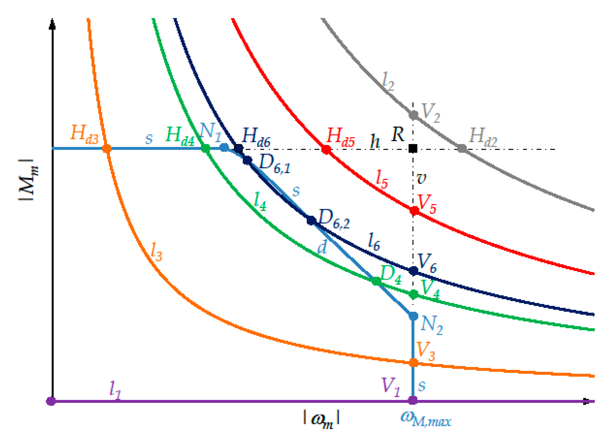
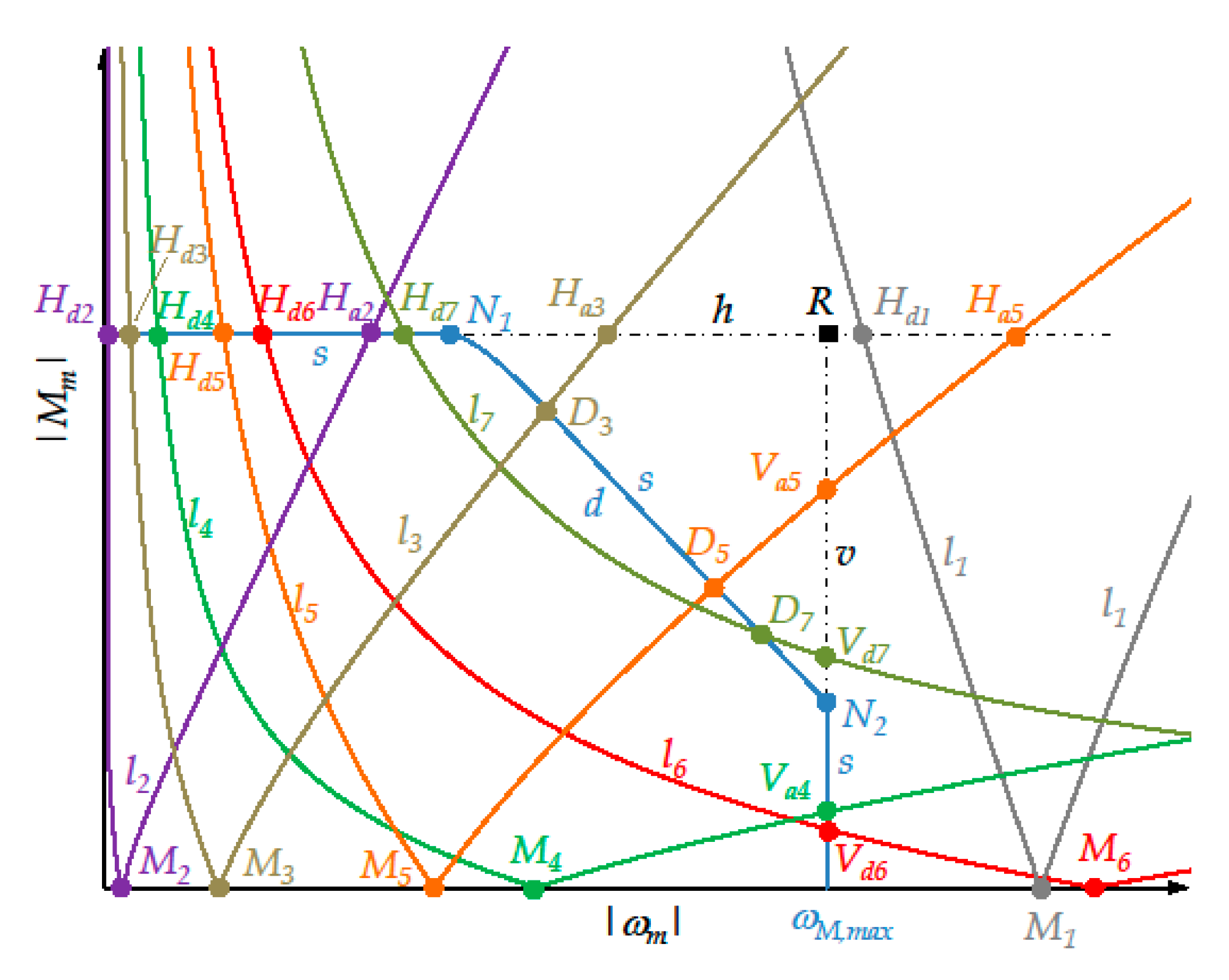
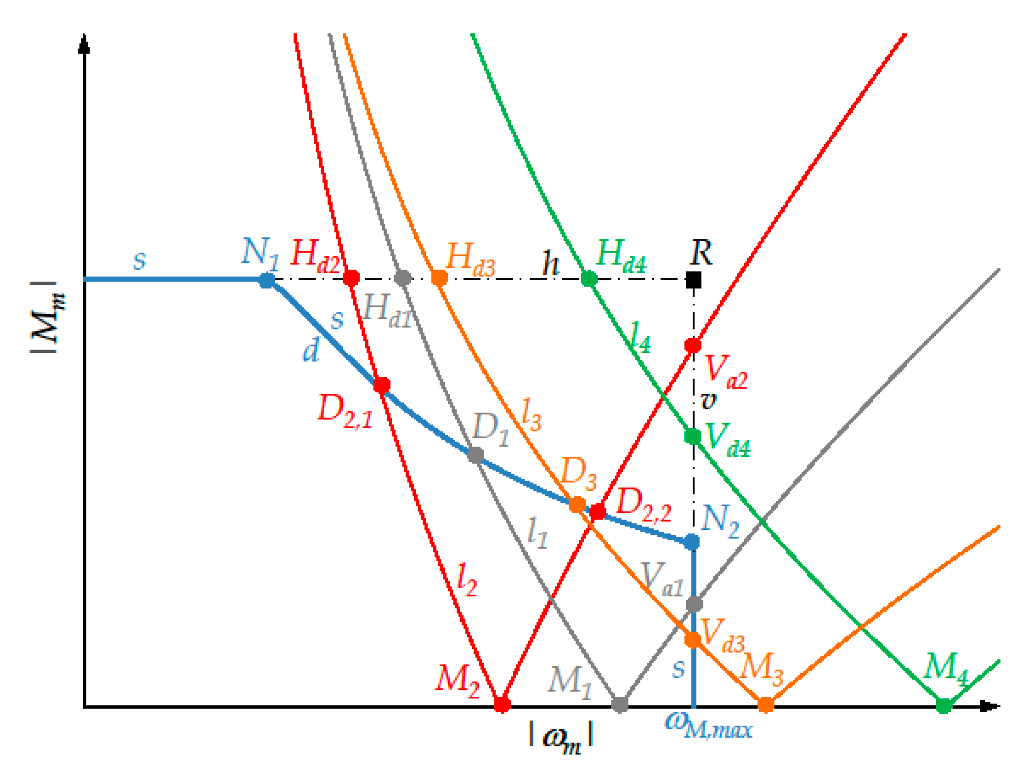
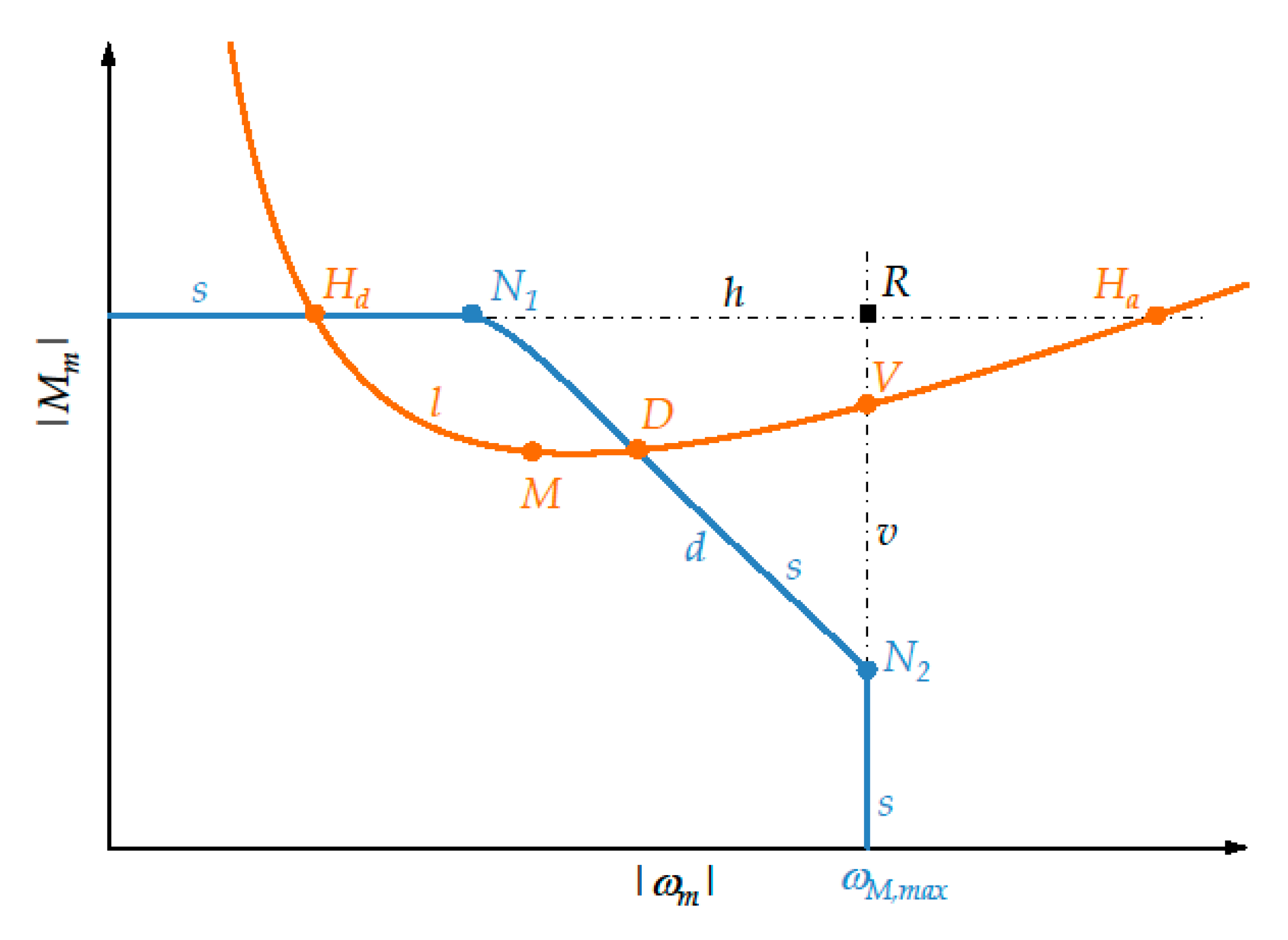
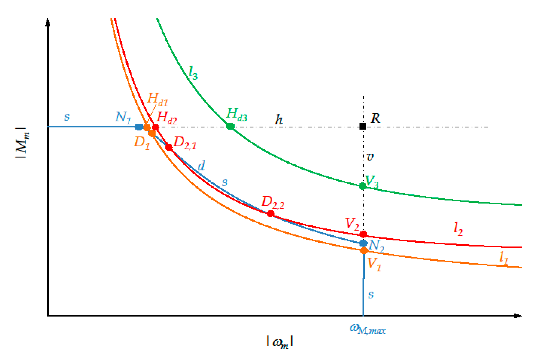
Since the purpose of the analysis at a given time instant t is to find the transmission ratio range [ τ m i n ( t ) ,   τ m a x ( t ) ] corresponding to the given motor at that time, this interval will be obtained by means of equations that directly involve the variable τ. Conversely, for a better graphic explanation, the figures will refer to the | ω m | | M m | plane, where the instantaneous load torque curve l, given by Equation (11), will be compared with the limit curve s of the dynamic operating range of the motor.
In general, as shown in Figure 8, curve l shows a descending arc, a minimum point M, and an ascending arc. The following intersection points will be used in the explanation of the new approach:
-
H d and H a denote the intersections, if exist, between the instantaneous load torque curve l and the horizontal straight-line h (see Figure 2) whose ordinate is M m , d y n , 1 . In particular, H d is the intersection of the descending arc of l, while H a is that of the ascending arc. Obviously, H d lies to the left of H a .
-
D denotes any intersection of l with the descending arc d of the limit curve of the dynamic operating range of the motor.
-
V denotes the only intersection of l with the vertical straight-line v whose abscissa is ω M , m a x .
The transmission ratio at the intersection H d is τ H d and at H a is τ H a . These transmission ratios are determined by means of the following equation
M M , d y n , 1 = | J M τ α l ( t ) + M l ( t ) τ |
that can be written as
τ M M , d y n , 1 = | J M α l ( t ) + M l ( t ) τ 2 |
Equation (29) can be solved as a second-degree algebraic equation in the unknown τ. It is noteworthy that τ H d is greater than τ H a .
The values of τ at the intersection points between the instantaneous load torque curve l and the descending arc d are determined by means of the following equation
M M , d y n ( τ ;   t ) = | J M τ α l ( t ) + M l ( t ) τ |
that can be written as
τ M M , d y n ( τ ;   t ) = | J M α l ( t ) + M l ( t ) τ 2 |
If the theoretical expression of M M , d y n ( τ ;   t ) (Equation (23)) is considered, a fourth degree algebraic equation in the unknown τ2 must be solved. If a polynomial interpolation of the r-th degree is used for arc N 1 N 2 , Equation (31) can be solved as a (r+1)-th degree algebraic equation in the unknown τ.
The value τ V of τ at the intersection V between the instantaneous load torque curve l and the vertical straight-line v is determined by means of the following equation
τ V ( t ) = | ω l ( t ) | ω M , m a x
The corresponding ordinate is
M V ( t ) = | J M α l ( t ) | ω l ( t ) | ω M , m a x + M l ( t )   | ω l ( t ) | 1 ω M , m a x | = | J M α l ( t ) τ V ( t ) + M l ( t )   τ V ( t ) |
Furthermore, the value τ N 1 ( t ) of τ at the breakpoint N 1 of curve s is determined by means of the following equation
τ N 1 ( t ) = | ω l ( t ) | ω M , 1

7.2. Brief Explanation of the New Approach

In order to understand the general approach adopted for the determination of the intersections between curves l and s, the particular case in which
α L ( t ) M L ( t ) > 0
is now rapidly considered. For the details, see Appendix C, where this is indicated as case IV.
If inequality (35) is valid, bearing in mind Equation (11), the instantaneous load torque curve l has equation
| M m ( | ω m | ;   t ) | = J M | α l ( t ) ω l ( t ) | | ω m | + | M l ( t ) ω l ( t ) | 1 | ω m |
Curve l has a regular minimum M, whose ordinate is equal to 2 J M α l ( t ) M l ( t ) , and two asymptotes: the first is the ordinate axis, the second is the straight-line passing through the origin whose slope is equal to J M | α l ( t ) ω l ( t ) | . Furthermore, all the curve points have positive ordinate and positive concavity (i.e., upwards).
The solution of Equation (31) is time consuming; therefore, the procedure is organized so as to avoid, if possible, this calculation. This result is obtained by first analyzing:
  • If the exclusion of the motor is possible without calculating the intersections between curve l and arc d.
  • Otherwise, if both the intersections between curves l and s do not belong to arc d.
Hereafter, there is a brief explanation on how to find the intersections between curves l and s, which are particularly important in the development of the method proposed. First, the ordinate of the minimum point M is compared with M M , d y n , 1 . If it is greater, there is no intersection between curves l and s, and the motor must be excluded (curve l 1 in Figure 9). Otherwise, the two intersections H d and H a of l with the horizontal straight-line h are determined, together with the corresponding transmission ratios τ H d ( t ) and τ H a ( t ) . If H d lies to the right of R (curve l 2 ), there is no intersection between curves l and s and the motor must be excluded. Otherwise, the position of H d with respect to N 1 is examined. If H d lies to the left of N 1 curves l and s surely intersect in two points, the first point is H d and τ m a x ( t ) coincides with τ H d ( t ) (curves l 3 , l 4 , l 5 ). In order to find τ m i n ( t ) the position of H a with respect to N 1 is examined. If H a also lies to the left of N 1 , H a itself is the second intersection and τ m i n ( t ) coincides with τ H a ( t ) (curve l 3 ). If H a lies to the right of N 1 , the position of point V with respect to N 2 is examined. If V lies below N 2 the second intersection is just point V and τ m i n ( t ) is equal to τ V ( t ) (curve l 4 ). If the second intersection is neither H a nor V, it must be found as an intersection D between l and the descending arc d (curve l 5 ).
If the previous analysis has permitted neither the motor exclusion nor the determination of τ m i n ( t ) and τ m a x ( t ) , then H d lies between N 1 and R (Figure 10). In this condition, if point V lies below point N 2 , the second intersection between l and s is just point V and τ m i n ( t ) is equal to τ V ( t ) (curve l 1 ); the first intersection is now the only intersection D between l and d and τ m a x ( t ) is determined in correspondence to it (curve l 1 , intersection point D 1 ). Otherwise, i.e., if V lies above N 2 , the intersections between curves l and d lying along arc N 1 N 2 must be determined. If the intersection points are two ( D 2 , 1 and D 2 , 2 for curve l 2 ), τ m i n ( t ) and τ m a x ( t ) are determined in correspondence to them; on the contrary, i.e., if there is no intersection (curve l 3 ), the motor must be excluded.
After this brief explanation, the analysis in detail of the five main possible cases, according to the sign of α l ( t ) and M l ( t ) , is carried out in Appendix C.
Nevertheless, even though the drive system has never been excluded by applying this procedure at all the successive instants, the analysis is not finished yet. In fact, as already explained in Section 5.1, this fact is not sufficient to assure that the drive system is admissible. The maximum over time τ m i n * of the minimum transmission ratios τ m i n ( t ) (Equation (15)) and the minimum over time τ m a x * of the maximum transmission ratios τ m a x ( t ) (Equation (16)) must now be found: if τ m i n * is greater than τ m a x * , the motor must be excluded, otherwise [ τ m i n * ,   τ m a x * ] is the transmission ratio range associated with the motor in order to perform the reference task.
After all, the procedure here briefly described and largely explained in Appendix C was implemented in a calculation program for finding the result desired: either the motor exclusion or the corresponding transmission ratio range [ τ m i n * ,   τ m a x * ] .

8. Effect of Efficiency and Inertia of the Transmission

The efficiency and inertia of the transmission are now taken into consideration. As regards its energy dissipation, the reducer has two different efficiencies, according to the direction of the power that flows through it [9]. In fact, the power direction can be either direct or inverse. It is direct when it is from the motor to the load, and the corresponding efficiency is denoted by η d ; conversely, the power direction is inverse when it is from the load to the motor, and the corresponding efficiency is denoted by η i (Figure 1). In the ideal case, with no energy dissipation, the two efficiencies are equal and their value is one. In the real case, the direct and inverse efficiency meet the inequalities
η i < η d < 1
The inverse efficiency η i can also be negative, but this case is here excluded. This paper assumes that the two efficiencies do not depend on speed; this means that in the transmission there is a predominance of the dry friction.
As explained in [9], the conditions of direct and inverse power direction are discriminated by the sign of the power M l ( t ) ω l ( t ) on the load side of the transmission. For the computation of the instantaneous load torque curve, instead of the function M l ( t ) , a generalized load torque M l ( t ) , related to it, can be used, i.e., if
M l ( t ) ω l ( t ) > 0
then
M l ( t ) = M l ( t ) η d  
whereas if
M l ( t ) ω l ( t ) < 0
then
M l ( t ) = η i M l ( t )  
If the power M l ( t ) ω l ( t ) is equal to zero, different cases must be distinguished, as explained in [9].
The rotation equilibrium at the joint is now expressed by the relation
M m ( t ) τ = J M τ 2 α l ( t ) + M l ( t )
Taking into account its similarity with Equation (7), at a given instant, the absolute value of the motor torque can be considered a function of the transmission ratio τ, with t as a parameter
| M m ( τ ;   t ) | = | J M τ α l ( t ) + τ M l ( t ) |
and the corresponding instantaneous load torque curve l is now expressed by
| M m ( | ω m | ;   t ) | = | J M α l ( t ) | ω l ( t ) | | ω m | + M l ( t ) | ω l ( t ) | 1 | ω m | |
Different diagrams can be devised to help the designer to find the transmissions that can be coupled with a given drive-system: one of them is described hereafter. M l ( t ) depends on the two parameters η d and η i ; therefore, in the calculation program there are two cycles, one inside the other. In the internal cycle, for a given value of η i , the transmission ratio range [ τ m i n * ( η d ;   η i ) ,   τ m a x * ( η d ;   η i ) ] is obtained as a function of η d , with η i as a parameter and η d [ η i ,   1 ] : this means that η d decreases from one to η i , and for each value of η d the transmission ratio range, if exists, is obtained according to the above-explained procedure. The two curves
{ τ m i n * = τ m i n * ( η d ;   η i ) τ m a x * = τ m a x * ( η d ;   η i )
are drawn in the η d τ plane (Figure 11).
For a given inverse efficiency η i , the curves τ m i n * = τ m i n * ( η d ;   η i ) and τ m a x * = τ m a x * ( η d ;   η i ) , together with the two vertical lines whose abscissas are equal to η i and one, respectively, border an area that is the transmission admissibility area associated with η i .
In the external cycle, η i decreases starting from one and, for each value of η i , the internal cycle is elaborated. After the completion of the two cycles, the result is shown in Figure 12, which shows a family of hatched areas, with η i as a parameter.
A reducer, characterized by the three parameters τ T , η d , T and η i , T , is represented in the same plane by a point T whose coordinates are η d , T and τ T , respectively; point T is labeled by its inverse efficiency η i , T (Figure 13). If the representative point T of a reducer lies inside the admissibility area associated with its inverse efficiency η i , T , this reducer can be paired with the given drive system to execute the reference task: this is the case of transmission T 1 . Or else, the reducer must be excluded for the given motor, as is the case of transmissions T 2 and T 3 .
This diagram is the result sought: it offers the designer an overview of the transmissions that can be coupled with the given drive system in order to perform the reference task from the point of view of the torque peak of the motor. It is similar to that shown in Section 7 of [9] for a rectangular dynamic operating range, but for a non-rectangular dynamic operating range it is necessarily found by means of another approach. Furthermore, it is obtained by means of an automatic calculation program.
Actually, a reducer is also characterized by its moment of inertia J T , M on the motor side and J T , L on the load side. Taking these moments of inertia into consideration, Equation (8) becomes
M m ( t ) = J M " τ α l ( t ) + τ M l " ( t )
where
J M " = J M + J T , M
M l " ( t ) = { M l ( t ) + J T , L α l ( t ) η d   if   [ M l ( t ) + J T , L α l ( t ) ] ω l ( t )   > 0   η i [ M l ( t ) + J T , L α l ( t ) ]   if   [ M l ( t ) + J T , L α l ( t ) ] ω l ( t )   < 0
and [ M l ( t ) + J T , L α l ( t ) ] ω l ( t ) is the power on the load side of the transmission.
Therefore, the most interesting reducers must also be checked taking into account their inertia. In this case the same program can be used with J M " instead of J M and M l " ( t ) instead of M l ( t ) .
Nevertheless, bearing in mind that M m ( t ) is given by Equation (46) and | ω m ( t ) | by Equation (6), in this case it is perhaps easier to directly check whether, during the reference task, the corresponding locus of a point ( | ω m ( t ) | , | M m ( t ) | ) lies inside the dynamic operating range of the drive system.
Furthermore, it is clear that the diagram shown in Figure 13 can be generalized by drawing admissibility areas whose parameters are also J T , M or J T , L .
It is clear that the same calculation program mentioned in Section 7 for the case of an ideal transmission can be applied with small changes to the case of a real reducer.

9. Case Study

During a periodic reference task, a rotating load covers a total rotation equal to π/10 rad. The acceleration profile is plotted in Figure 14, while the corresponding speed profile is shown in Figure 15.
The load has a constant moment of inertia J L equal to 0.35 kg m2 and is subject to a constant resistant torque equal to 20.0 Nm. The total load torque M L is represented in Figure 16 as a function of time.
The characteristics of a drive system candidate to perform the reference task are summarized in Table 1.
Its dynamic operating range is drawn in Figure 17, with a limit curve that shows a descending arc N 1 N 2 .
By applying the method explained in [15] to a transmission with negligible inertia and no energy dissipation, Figure 18 shows the global load torque curve g associated with the reference task and the limit curve s of the dynamic operating range, both expressed in suitable coordinates.
According to [15], on curve g two arcs can be recognized:
-
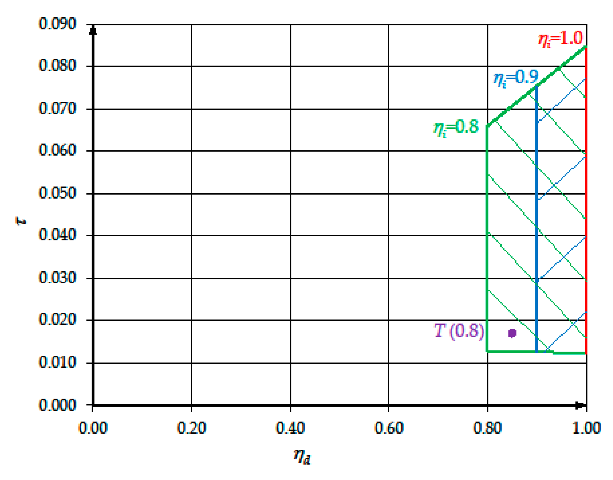
Arc PQ is a feasibility arc and corresponds to the transmission ratio range [ 1 / 70.93 ,   1 / 11.86 ] . This means that the motor is admissible and can surely be coupled with an ideal reducer whose transmission ratio lies in this range.
-
Arc QQ’ is an uncertainty arc and corresponds to the transmission ratio range [ 1 / 88.85 ,   1 / 7 0.93 ) . This means that, according to the method described in [15], the designer cannot ascertain if the motor can be coupled with an ideal reducer whose transmission ratio lies in this range. Therefore, this is a case for which the method proposed in this paper is particularly effective.
By making a polynomial interpolation of the descending arc d of curve s and applying the procedure described in Section 7 to an ideal transmission, a first obvious result is that the motor is admissible. Figure 19 shows the curves τ m i n = τ m i n ( t ) and τ m a x = τ m a x ( t ) . The admissible transmission ratio range [ τ m i n * ,   τ m a x * ] is equal to [ 1 / 80.58 ,   1 / 11.86 ] . This means that in the uncertainty arc QQ’ there is an arc QF, which corresponds to the transmission ratio range [ 1 / 80.58 ,   1 / 70.93 ] , that is admissible, and another arc FQ’, which corresponds to the transmission ratio range [ 1 / 88.85 ,   1 / 80.58 ] , that is not admissible.
Taking also into account the reducer efficiencies, but neglecting its inertia, Figure 20 shows three transmission admissibility areas.
The characteristics of a transmission candidate to move the joint are summarized in Table 2. Its moment of inertia J T , L on load side is negligible with respect to J L .
Figure 20 also shows the representative point T of this reducer. Since point T lies inside the admissibility area associated with its inverse efficiency η i , T , the transmission considered seems admissible.
Figure 21 shows the transmission admissibility areas when the reducer inertia is taken into account. Point T still lies in the admissibility area associated with the transmission inverse efficiency η i , T . Figure 22 shows that during the reference task the corresponding locus of a point ( | ω m ( t ) | , | M m ( t ) | ) , obtained as explained at the end of Section 8, lies inside the dynamic operating range of the drive system.
Both Figure 21 and Figure 22 confirm that the transmission candidate to move the joint can be coupled with the motor taken into consideration in order to perform the reference task from the point of view of the torque peak of the drive system. It is clear that another analysis from the point of view of the motor thermal problem must be carried out in order to ascertain the complete admissibility of this motor-transmission couple.

10. Conclusions

In mechatronic applications, a load is often driven by a converter-motor system whose limit curve of the dynamic operating range is non-rectangular: i.e., this curve shows a descending arc d. This particular shape makes it more difficult to choose the motor-transmission couple to perform the reference task. In this case, so far no method offers the designer a complete overview of which transmissions can be coupled with the given drive system, unless every drive system–reducer couple be checked: during the reference task the corresponding locus of a point | ω m | | M m | must lie inside the dynamic operating range of the drive system.
To this end, the contribution of this paper is to propose an original method: for a given drive system, the design process is based on a succession of instant analyses; at each instant the comparison between the limit curve of its dynamic operating range and an instantaneous load torque curve permits the designer to find their intersections, if exist. To this end, an equation of the descending arc d is required: this is obtained either by elaborating the equations governing the drive system and using its catalog parameters or through a polynomial interpolation of the catalog graphic curve. For ideal transmissions—i.e., with negligible inertia and no energy dissipation—the entire analysis either permits the exclusion of the drive system or provides the range [ τ m i n * ,   τ m a x * ] of the transmission ratios that can be coupled with it.
The same approach is then extended taking also into account the energy dissipation of the reducer—i.e., its direct efficiency η d and inverse efficiency η i . It is noteworthy that in mechatronic applications the case of alternation of direct and inverse power flow through the transmission is frequent. An automatic calculation program generates a diagram in which a family of areas correlating transmission ratio, and direct and inverse efficiency of the reducer is drawn. A point T represents each transmission and this can be coupled with the given drive system in order to perform the reference task if T lies within the appropriate area. The transmission inertia can also be kept into account in this diagram. Therefore, for a generic drive system of the above-mentioned type this method provides the result desired, which is a diagram that shows all the transmissions that permit the motor to perform the reference task.
The method proposed proves rapid and effective for any drive system whose limit curve of the dynamic operating range depends on the motor speed. In particular, as shown for the case studied in Section 9, it is effective for those motors for which the method explained in [15] either does not give any solution or only gives a partial solution.

Funding

This research received no external funding.

Conflicts of Interest

The authors declare no conflict of interest.

Nomenclature

I ¯ [A]current phasor in the equivalent two-phase motor
I d [A]direct component of current in the equivalent two-phase motor
I q [A]quadrature component of current in the equivalent two-phase motor
I m a x [A]saturation value of current in the equivalent two-phase motor
I m a x , c o n v [A]saturation value of current in the drive system (maximum rms current in the three-phase motor)
K E [V/rad/s]voltage constant of the motor (rms line to line voltage in the three-phase motor)
K E , q [V/rad/s]voltage constant of the equivalent two-phase motor
K T , q [Nm/A]torque constant of the equivalent two-phase motor
J M [kg m2]moment of inertia of the motor
J T , L [kg m2]moment of inertia of the transmission on load side
J T , M [kg m2]moment of inertia of the transmission on motor side
L s [H]synchronous inductance
M l [Nm]load torque
M m [Nm]current motor torque
M M , d y n [Nm]limit torque of the dynamic operating range
M M , S 1 [Nm]limit torque of the continuous duty operating range
n [-]number of pole pairs
R p h [Ω]phase resistance
t [s]time
V ¯ [V]voltage phasor in the equivalent two-phase motor
V d [V]direct component of voltage in the equivalent two-phase motor
V q [V]quadrature component of voltage in the equivalent two-phase motor
V m a x [V]saturation value of voltage in the equivalent two-phase motor (rms line to line voltage in the three-phase motor)
Z [Ω]absolute value of the phase impedance in the equivalent two-phase motor
α l [rad/s2]load angular acceleration
η d [-]direct efficiency of transmission
η i [-]inverse efficiency of transmission
τ [-]transmission ratio
Ψ [Wb]permanent magnet flux
ω [s−1]electrical frequency
ω l [rad/s]load angular speed
ω m [rad/s]motor angular speed

Appendix A

This appendix considers the case in which the flux-weakening technique is not applied [16] and provides the equation of the descending arc w of the limit curve s of the dynamic operating range of the drive system and the expression of ω M , 1 .
In general, in steady state conditions a two-phase motor is subject to a voltage phasor V ¯ whose components V d and V q along the rotor axes d (direct) and q (quadrature) satisfy the following equations
{ V d = R p h I d ω L s I q V q = R p h I q + ω L s I d + Ψ ω
where ω is the electrical frequency and I d and I q are the components of the current phasor I ¯ along the rotor axes d and q.
The relation between the electrical frequency ω and the motor speed ω m is
ω = n ω m
where n is the number of pole pairs.
Indicating by K T , q the two-phase motor torque constant, this is equal to
K T , q = Ψ n
and the motor torque M m is equal to
M m = K T , q I q
and does not depend on I d .
The voltage constant of the two-phase motor is denoted by K E , q and is equal to
K E , q = K T , q = Ψ n
It is also equal to the voltage constant K E of the three-phase motor, directly found in the drive system catalog
K E , q = K T , q = K E
The squared impedance Z 2 of a phase is
Z 2 = R p h 2 + ω 2 L s 2 = R p h 2 + n 2 ω m 2 L s 2
If the flux-weakening technique is not applied, I d is maintained equal to zero, so that Equation (A1) become
{ V d = ω L s I q V q = R p h I q +   Ψ ω
Indicating by V m a x the saturation voltage, when saturation occurs V d and V q satisfy the following condition
V d 2 + V q 2 = V m a x 2
Taking into account Equations (A7) and (A9) and squaring and summing Equations (A8), the following equation is obtained
V m a x 2 = Z 2 I q 2 + 2 Ψ ω R p h I q + Ψ 2 ω 2
This is a second-degree equation in the unknown I q , whose solution, for positive values of I q , i.e., of the motor torque M m , is
I q = Ψ ω R [ 1 + ( V m a x 2 Ψ 2 ω 2 ) Z 2 ( Ψ ω R ) 2 1 ] Z 2
Hence, the saturation value M M , d y n of the motor torque as a function of ω is equal to
M M , d y n ( ω ) = K T , q Ψ ω R p h [ 1 + ( V m a x 2 Ψ 2 ω 2 ) Z 2 Ψ 2 ω 2 R p h 2 1 ] Z 2
Taking into account Equations (A2), (A5), and (A6), M M , d y n becomes a function of the absolute value of the motor speed | ω m |
M M , d y n ( | ω m | ) = K E 2 R p h R p h 2 Z 2 ( ω m ) | ω m | [ 1 + ( V m a x 2 K E 2 ω m 2 ) K E 2 ω m 2 R p h 2 Z 2 ( ω m ) 1 ]
which is the equation sought.
Substituting for | ω m | from Equation (6) into Equation (A13), M M , d y n becomes a function of the transmission ratio τ, with t as a parameter:
M M , d y n ( τ ;   t ) = K E 2 R p h R p h 2 R p h 2 + n 2 ω l 2 ( t ) τ 2 L s | ω l ( t ) | τ [ 1 + [ V m a x 2 K E 2 ω l 2 ( t ) τ 2 ] K E 2 ω l 2 ( t ) τ 2 R p h 2 R p h 2 + n 2 ω l 2 ( t ) τ 2 L s 1 ]
After some simplifications, Equation (A14) becomes
M M , d y n ( τ ;   t ) = K E 2 R p h R p h 2 τ 2 R p h 2 + n 2 ω l 2 ( t ) L s τ | ω l ( t ) | [ 1 + 1 τ 2 [ τ 2 V m a x 2 K E 2 ω l 2 ( t ) ] K E 2 ω l 2 ( t ) R p h 2 τ 2 R p h 2 + n 2 ω l 2 ( t ) L s 1 ]
The expression of speed ω M , 1 as a function of the motor electrical parameters can be found by observing that at this speed the quadrature current I q is equal to I m a x . After having set this value, Equation (A10) becomes
V m a x 2 = ( R p h 2 + ω 2 L s 2 ) I m a x 2 + 2 Ψ ω R p h I m a x + Ψ 2 ω 2
This is a second-degree equation in ω, whose solution is
ω 1 = R p h I m a x Ψ L s 2 I m a x 2 + Ψ 2 [ 1 + ( V m a x 2 R p h 2 I m a x 2 ) ( L s 2 I m a x 2 + Ψ 2 ) R p h 2 I m a x 2 Ψ 2 1 ]
Taking into account Equations (A2), (A5) and (A6), ω M , 1 is given by
ω M , 1 = R p h I m a x K E n 2 L s 2 I m a x 2 + K E 2 [ 1 + ( V m a x 2 R p h 2 I m a x 2 ) ( n 2 L s 2 I m a x 2 + K E 2 ) R p h 2 I m a x 2 K E 2 1 ]

Appendix B

This appendix considers the case in which the flux-weakening technique is applied in order to broaden the dynamic operating range of the drive system [16]. It provides the equation of the descending arc d of the limit curve s of the dynamic operating range and the expression of ω M , 1 . Equations (A1)–(A7) are still valid.
Indicating by V m a x the saturation value of voltage and by I m a x that of current, in saturation conditions for both voltage and current, their components meet the following equations
{ V d 2 + V q 2 = V m a x 2 I d 2 + I q 2 = I m a x 2
Taking into account Equation (A1) and (A7) and squaring and summing Equations (A19), the following equation is obtained
V m a x 2 = Z 2 I m a x 2 + 2 Ψ ω 2 L s I d + 2 Ψ ω R p h I q + Ψ 2 ω 2
Bearing in mind Equation (A20), the direct current Id assumes the following expression
I d = [ V m a x 2 Z 2 I m a x 2 Ψ 2 ω 2 ] ( 2 R p h Ψ ω ) I q 2 ω 2 L s Ψ
Substituting for I d from Equation (A21) into the second of Equation (A19), a second-degree equation in the unknown I q is obtained
[ 4 Z 2 Ψ 2 ω 2 ] I q 2 2 [ V m a x 2 Z 2 I m a x 2 Ψ 2 ω 2 ] ( 2 R p h Ψ ω ) I q + [ V m a x 2 Z 2 I m a x 2 Ψ 2 ω 2 ] 2 4 ω 2 L s 2 Ψ 2 ω 2 I m a x 2 = 0
For positive values of I q , i.e., of the motor torque M m , its solution is
I q = [ V m a x 2 Z 2 I m a x 2 Ψ 2 ω 2 ] ( R p h Ψ ω ) 2 Ψ 2 ω 2 Z 2 + L s Ψ ω 2 4 Z 2 I m a x 2 Ψ 2 ω 2 [ V m a x 2 Z 2 I m a x 2 Ψ 2 ω 2 ] 2 2 Ψ 2 ω 2 Z 2
Taking into account Equations (A3) and (A4), the saturation value M M , d y n of the motor torque, as a function of ω , is equal to
M M , d y n ( ω ) = n R p h [ V m a x 2 Z 2 I m a x 2 Ψ 2 ω 2 ] 2 ω Z 2 + n   ω L s 4 Z 2 I m a x 2 Ψ 2 ω 2 [ V m a x 2 Z 2 I m a x 2 Ψ 2 ω 2 ] 2 2 ω Z 2
Bearing in mind Equations (A2), (A5), and (A6), M M , d y n becomes a function of the absolute value of motor speed | ω m |
M M , d y n ( | ω m | ) = R p h [ V m a x 2 K E 2 ω m 2 Z 2 ( ω m ) I m a x 2 ] 2 | ω m | Z 2 ( ω m ) + n | ω m | L s 4 Z 2 ( ω m ) I m a x 2 K E 2 ω m 2 [ V m a x 2 K E 2 ω m 2 Z 2 ( ω m ) I m a x 2 ] 2 2 | ω m | Z 2 ( ω m )
This is the equation desired.
Substituting for | ω m | from Equation (6) into Equation (A25), M M , d y n becomes a function of the transmission ratio τ, with t as a parameter:
M M , d y n ( τ ;   t ) = R p h { V m a x 2 K E 2 ω l 2 ( t ) τ 2 [ R p h 2 + n 2 L s 2 ω l 2 ( t ) τ 2 ] I m a x 2 } 2 | ω l ( t ) | τ [ R p h 2 + n 2 L s 2 ω l 2 ( t ) τ 2 ] + | ω l ( t ) | τ n L s 4 [ R p h 2 + n 2 L s 2 ω l 2 ( t ) τ 2 ] I m a x 2 K E 2 ω l 2 ( t ) τ 2 { V m a x 2 K E 2 ω l 2 ( t ) τ 2 [ R p h 2 + n 2 L s 2 ω l 2 ( t ) τ 2 ] I m a x 2 } 2 2 | ω l ( t ) | τ [ R p h 2 + n 2 L s 2 ω l 2 ( t ) τ 2 ]
After some simplifications, the same expression becomes
M M , d y n ( τ ;   t ) = τ R p h { [ τ 2 V m a x 2 K E 2 ω l 2 ( t ) ] [ τ 2 R p h 2 + n 2 L s 2 ω l 2 ( t ) ] I m a x 2 } 2 | ω l ( t ) | [ τ 2 R p h 2 + n 2 L s 2 ω l 2 ( t ) ] + n L s 4 [ τ 2 R p h 2 + n 2 L s 2 ω l 2 ( t ) ] I m a x 2 K E 2 ω l 2 ( t ) { [ τ 2 V m a x 2 K E 2 ω l 2 ( t ) ] [ τ 2 R p h 2 + n 2 L s 2 ω l 2 ( t ) ] I m a x 2 } 2 2 [ τ 2 R p h 2 + n 2 L s 2 ω l 2 ( t ) ]
The expression of speed ω M , 1 as a function of the motor electrical parameters can be found by observing that at this speed the direct current I d is still equal to zero, whereas the quadrature current I q is equal to I m a x . After having set these values, Equation (A20) becomes
( L s 2 I m a x 2 + Ψ 2 ) ω 2 + 2 R p h I m a x Ψ ω ( V m a x 2 R p h 2 I m a x 2 ) = 0
This is a second-degree equation in ω whose solution, bearing in mind Equation (A5), is
ω 1 = 1 n R p h I m a x K E n 2 L s 2 I m a x 2 + K E 2 [ 1 + ( V m a x 2 R p h 2 I m a x 2 ) ( n 2 L s 2 I m a x 2 + K E 2 ) ( R p h I m a x K E ) 2 1 ]
Taking into account Equations (A2) and (A6), ω M , 1 is given by
ω M , 1 = R p h I m a x K E n 2 L s 2 I m a x 2 + K E 2 [ 1 + ( V m a x 2 R p h 2 I m a x 2 ) ( n 2 L s 2 I m a x 2 + K E 2 ) ( R p h I m a x K E ) 2 1 ]
This equation gives the same value of ω M , 1 as in Equation (A18). At ω M , 1 M M , d y n ( | ω m | ) shows a regular maximum equal to M M , d y n , 1 .

Appendix C

This appendix shows how to find the intersections between the instantaneous load torque curve l(t) and the limit curve s of the dynamic operating range of the drive system. According to the sign of α l ( t ) and M l ( t ) , five possible cases are considered.
( I ) { α l ( t ) = 0 M l ( t ) = 0
In the trivial case in which α l ( t ) and M l ( t ) are simultaneously null, | M m ( t ) | is null (Figure A1, curve l 1 ), i.e., function | M m ( | ω m | ;   t ) | is a constant with null ordinate and the motor cannot be excluded at this instant: therefore, ω m , m i n ( t ) is equal to zero and ω m , m a x ( t ) is equal to ω M , m a x . As a consequence,
τ m i n ( t ) = τ V ( t )
and is given by Equation (32), whereas, taking into account Equation (13), τ m a x ( t ) tends to +∞.
Figure A1. Intersections between the instantaneous load torque curve l and the non-rectangular dynamic operating range of the motor: cases I and II.
Machines 07 00054 g0a1
( II ) { α l ( t ) = 0 M l ( t ) 0
In this case, Equation (28) becomes
M M , d y n , 1 = | M l ( t ) | τ
and the instantaneous load torque curve l is a descending equilateral hyperbola (Figure A1). There is only one intersection between curve l and the horizontal straight-line h, and the corresponding transmission ratio is
τ H d ( t ) = M M , d y n , 1 | M l ( t ) |
The intersection V between curve l and the vertical straight-line v corresponds to the transmission ratio τ V ( t ) given by Equation (32) and its ordinate M V ( t ) is equal to
M V ( t ) = | M l ( t ) | τ V ( t ) = | M l ( t ) | | ω l ( t ) | ω M , m a x
Different sub-cases are possible:
(A)
If H d does not lie to the left of R (Figure A1, curve l 2 ), i.e., if
τ H d ( t ) τ V ( t )
the motor must be excluded.
(B)
Otherwise [ τ H d ( t ) > τ V ( t ) ]
(1)
If H d does not lie to the right of N 1 , i.e., if
τ H d ( t ) τ N 1 ( t )
then the first intersection between curves l and s coincides with H d , and
τ m a x ( t ) = τ H d ( t ) = M M , d y n , 1 | M l ( t ) |
As regards the second intersection, there are two sub-cases:
(a)
If point V does not lie above N 2 (Figure A1, curve l 3 ), i.e., if
M V ( t ) M M , d y n , 2
then the second intersection coincides with V, and τ m i n ( t ) is given by τ V ( t ) (Equation (32))
τ m i n ( t ) = τ V ( t )
(b)
Otherwise [ M V ( t ) > M M , d y n , 2 ] (Figure A1, curve l 4 ) the second intersection of curve l with curve s belongs to arc d and the corresponding transmission ratio, i.e., τ m i n ( t ) , must be calculated by solving Equation (31) and lies in the range ( τ V ( t ) ,   τ N 1 ( t ) ) .
(2)
Otherwise H d lies to the right of N 1 and to the left of R, i.e.,
τ V ( t ) <   τ H d ( t ) <   τ N 1 ( t )
Two sub-cases are possible:
(a)
If point V does not lie above N 2 , i.e., if inequality (A40) is met, the second intersection coincides with V and τ m i n ( t ) is given by Equation (A41), while the first intersection of curve l with curve s belongs to arc d. The corresponding transmission ratio, i.e., τ m a x ( t ) , must be calculated by solving Equation (31) and lies in the range ( τ V ( t ) ,   τ N 1 ( t ) ) .
(b)
Otherwise [ M V ( t ) > M M , d y n , 2 ] the intersections between curves l and d that lie along arc d must be calculated by solving Equation (31):
  • If there is no intersection, the motor must be excluded (Figure A1, curve l 5 ).
  • Otherwise these intersections are two, lie in the range ( τ V ( t ) ,   τ N 1 ( t ) ) and their corresponding transmission ratios are τ m i n ( t ) and τ m a x ( t ) (Figure A1, curve l 6 ).
    ( III ) { α l ( t ) 0 M l ( t ) = 0
In this case Equation (28) becomes
M M , d y n , 1 = J M | α l ( t ) | 1 τ
and the instantaneous load torque curve l is an ascending straight-line passing through the origin with slope J M | α l ( t ) | / | ω l ( t ) | (Figure A2). At the instant considered, the motor cannot be excluded. The first intersection between curves l and s is at null speed, so that, bearing in mind Equation (13), τ m a x ( t ) tends to + . Curve l intersects the horizontal straight-line h at point H a and the corresponding transmission ratio is
τ H a ( t ) = J M | α l ( t ) | M M , d y n , 1
Figure A2. Intersections between the instantaneous load torque curve l and the non-rectangular dynamic operating range of the motor: case III.
Machines 07 00054 g0a2
As regards the second intersection between curves l and s
(A)
If H a does not lie to the right of N 1 (Figure A2, curve l 1 ), i.e., if
τ H a ( t ) τ N 1 ( t )
then the second intersection coincides with H a and τ m i n ( t ) is given by
τ m i n ( t ) = τ H a ( t ) = J M | α l ( t ) | M M , d y n , 1
(B)
Otherwise ( H a lies to the right of N 1 )
(1)
If V does not lie above N 2 (Figure A2, curve l 2 ), i.e., if inequality (A40) is met, then the second intersection between curves l and s coincides with V and τ m i n ( t ) is given by Equation (A41).
(2)
Otherwise H a lies to the right of N 1 and V lies above N 2 (Figure A2, curve l 3 ), i.e.
{ τ H a ( t ) < τ N 1 ( t ) M V ( t ) > M M , d y n , 2
and the second intersection of curves l and s belongs to arc d. The corresponding transmission ratio τ m i n ( t ) must be calculated by solving Equation (31) and lies in the range ( τ V ( t ) ,   τ N 1 ( t ) ) .
( IV )   α l ( t ) M l ( t ) > 0
that is either
{ α l ( t ) > 0 M l ( t ) > 0
or
{ α l ( t ) < 0 M l ( t ) < 0
In this case, taking into account Equation (11), the instantaneous load torque curve l has equation
| M m ( | ω m | ;   t ) | = J M | α l ( t ) ω l ( t ) | | ω m | + | M l ( t ) ω l ( t ) | 1 | ω m |
and Equation (10) becomes
| M m ( τ ;   t ) | = J M | α l ( t ) | τ + | M l ( t ) | τ
Curve l has a regular minimum M and two asymptotes: the first is the vertical axis, when | ω m | tends to 0: in this case all the motor power is used to balance the load; the second is coincident with the straight-line passing through the origin whose slope is equal to J M | α l ( t ) ω l ( t ) | , when | ω m | tends to +∞: in this condition all the motor power is used to accelerate the motor itself. The abscissa of the minimum point M is equal to
| ω m | M = M l ( t ) J M α l ( t ) | ω l ( t ) |
and its ordinate is equal to
| M m | M = 2 J M α l ( t ) M l ( t )
In this condition, the motor distributes its power in equal parts between the motor itself and the load.
Furthermore, all the curve points have positive ordinate and positive concavity (i.e., upwards).
Equation (28) becomes
M M , d y n , 1 = J M | α l ( t ) | τ + | M l ( t ) | τ
and then the two intersections with the horizontal straight-line h, if they exist, correspond to the transmission ratios
τ H d ( t ) = M M , d y n , 1 + M M , d y n , 1 2 4 J M α l ( t ) M l ( t ) 2 | M l ( t ) |
and
τ H a ( t ) = M M , d y n , 1 M M , d y n , 1 2 4 J M α l ( t ) M l ( t ) 2 | M l ( t ) |
Different sub-cases are possible:
(A)
If the minimum point M of curve l lies above the horizontal straight-line h, i.e., if
2 J M α l ( t ) M l ( t ) > M M , d y n , 1
the motor must be excluded (Figure 9, curve l 1 ).
(B)
Otherwise
(1)
If H d does not lie to the left of R, i.e., if inequality (A37) is met, the motor must be excluded (Figure 9, curve l 2 ).
(2)
Otherwise if H d does not lie to the right of N 1 , i.e., if inequality (A38) is met, at the instant considered the motor is admissible and H d is the first intersection between curves l and s, so that
τ m a x ( t ) = τ H d ( t ) = M M , d y n , 1 + M M , d y n , 1 2 4 J M α l ( t ) M l ( t ) 2 | M l ( t ) |
As regards the second intersection of curves l and s:
(a)
If H a does not lie to the right of N 1 , i.e., if Equation (A46) is met, the second intersection coincides with H a (Figure 9, curve l 3 ) and
τ m i n ( t ) = τ H a ( t ) = M M , d y n , 1 M M , d y n , 1 2 4 J M α l ( t ) M l ( t ) 2 | M l ( t ) |
(b)
Otherwise (if H a lies to the right of N 1 ) there are two sub-cases:
  • If point V does not lie above N 2 (Figure 9, curve l 4 ), i.e., if inequality (A40) is met, the second intersection coincides with V and τ m i n ( t ) is given by Equation (A41).
  • Otherwise [ M V ( t ) > M M , d y n , 2 ] (Figure 9, curve l 5 ) the second intersection belongs to arc d and the corresponding transmission ratio τ m i n ( t ) must be calculated by solving Equation (31) and lies in the range ( τ V ( t ) ,   τ N 1 ( t ) ) .
(3)
Otherwise H d lies to the right of N 1 , i.e., inequalities (A42) are met. Some subcases are possible:
(a)
If point V does not lie above N 2 (Figure 10, curve l 1 ), i.e., if inequality (A40) is met, then the second intersection of curves l and s coincides with V and τ m i n ( t ) is given by Equation (A41), while the first intersection belongs to arc d. The corresponding transmission ratio τ m a x ( t ) must be calculated by solving Equation (31) and lies in the range ( τ V ( t ) ,   τ N 1 ( t ) ) .
(b)
Otherwise [ M V ( t ) > M M , d y n , 2 ] the intersections between curve l and arc N 1 N 2 must be calculated by solving Equation (31):
  • If there is no intersection, the motor must be excluded (Figure 10, curve l 3 ).
  • Otherwise the intersections are two and τ m i n ( t ) and τ m a x ( t ) lie in the range ( τ V ( t ) ,   τ N 1 ( t ) ) (Figure 10, curve l 2 ).
( V ) α l ( t ) M l ( t ) < 0
that is either
{ α l ( t ) > 0 M l ( t ) < 0
or
{ α l ( t ) < 0 M l ( t ) > 0
In the | ω m | | M m | plane the instantaneous load torque curve l is continuous and has the same two asymptotes already seen for the previous case, but the shape of curve l is different (Figure A3). In fact, its first derivative is discontinuous at the minimum point M, which is an edge point, whose abscissa is equal to
| ω m | M = M l ( t ) J M α l ( t ) | ω l ( t ) |
and whose ordinate is null. At this point the derivative of the kinetic energy of the motor is used to win the load, whereas the motor does not exert any torque. The transmission ratio τ M ( t ) corresponding to point M is equal to
τ M ( t ) = J M α l ( t ) M l ( t )
Figure A3. Intersections between the instantaneous load torque curve l and the non-rectangular dynamic operating range of the motor: case V (some subcases).
Machines 07 00054 g0a3
Curve l is made up of two different arcs, one descending and the other ascending, with two different equations. The descending arc l d of curve l has equation
| M m ( | ω m | ;   t ) | = J M | α l ( t ) ω l ( t ) | | ω m | + | M l ( t ) ω l ( t ) | 1 | ω m | with   | ω m | | M l ( t ) | J M | α l ( t ) |   | ω l ( t ) |
and the corresponding equation in the unknown τ is
| M m | = J M | α l ( t ) | 1 τ + | M l ( t ) | τ with   τ J M | α l ( t ) | | M l ( t ) |
Bearing in mind Equation (28), the intersection H d of the descending arc l d with the horizontal straight-line h corresponds to the transmission ratio
τ H d ( t ) = M M , d y n , 1 + M M , d y n , 1 2 4 J M α l ( t ) M l ( t ) 2 | M l ( t ) |
The ascending arc l a of curve l has equation
| M m ( | ω m | ;   t ) | = + J M | α l ( t ) ω l ( t ) | | ω m | | M l ( t ) ω l ( t ) | 1 | ω m | with   | ω m | | M l ( t ) | J M | α l ( t ) |   | ω l ( t ) |
and the corresponding equation in the unknown τ is
| M m | = + J M | α l ( t ) | 1 τ | M l ( t ) | τ with   τ J M | α l ( t ) | | M l ( t ) |
Taking into account Equation (28), the intersection H a of the ascending arc l a with the horizontal straight-line h corresponds to the transmission ratio
τ H a ( t ) = M M , d y n , 1 + M M , d y n , 1 2 4 J M α l ( t ) M l ( t ) 2 | M l ( t ) |
Furthermore, the intersections V d and V a between the vertical straight-line v and arcs l d and l a , respectively, must be considered. Their ordinates are
M V d = J M | α l ( t ) | 1 τ V ( t ) + | M l ( t ) | τ V ( t ) if   τ M ( t ) τ V ( t )
M V a = + J M | α l ( t ) | 1 τ V ( t ) | M l ( t ) | τ V ( t ) if   τ M ( t ) τ V ( t )
respectively.
Different sub-cases are possible:
(A)
If H d does not lie to the left of R, i.e., if inequality (A37) is met, then the motor must be excluded (Figure A3, curve l 1 ).
(B)
Otherwise
(1)
If H d does not lie to the right of N 1 , i.e., if inequality (A38) is met, then at the instant considered the motor is admissible and the first intersection between curves l and s coincides with H d , so that
τ m a x ( t ) = τ H d ( t )
given by Equation (A69).
As regards the second intersection of curves l and s:
(a)
If H a does not lie to the right of N 1 , i.e., if Equation (A46) is met, the second intersection coincides with H a (Figure A3, curve l 2 ), and
τ m i n ( t ) = τ H a ( t )
given by Equation (A72).
(b)
Otherwise, if H a does not lie to the right of R (Figure A3, curve l 3 ), i.e., if
τ V ( t ) τ H a ( t ) < τ N 1 ( t )
the second intersection coincides with the intersection between the ascending curve l a and arc d. Its transmission ratio, i.e., τ m i n ( t ) , must be calculated by solving Equation (31) and lies in the range ( τ V ( t ) ,   τ N 1 ( t ) ) .
(c)
Otherwise ( H a lies to the right of R) there are some sub-cases:
(1)
If the edge-point M does not lie to the right of R, i.e., if
τ M ( t ) τ V ( t )
the second intersection belongs to the ascending curve l a , with two sub-cases:
(a)
If point V V a does not lie above N 2 , i.e., if
M V a ( t ) M M , d y n , 2
the second intersection coincides with V (Figure A3, curve l 4 ) and τ m i n ( t ) is given by Equation (A41).
(b)
Otherwise [ M V a ( t ) > M M , d y n , 2 ] (Figure A3, curve l 5 ) the second intersection coincides with the intersection between the ascending curve l a and arc d. Its transmission ratio, i.e., τ m i n ( t ) , must be calculated by solving Equation (31) and lies in the range ( τ V ( t ) ,   τ N 1 ( t ) ) .
(2)
Otherwise (the edge point M lies to the right of R), the second intersection belongs to the descending curve l d with two sub-cases:
(a)
If point V V d does not lie above N 2 , i.e., if
M V d ( t ) M M , d y n , 2
the second intersection coincides with V (Figure A3, curve l 6 ) and τ m i n ( t ) is given by Equation (A41).
(b)
Otherwise [ M V d ( t ) > M M , d y n , 2 ] the second intersection coincides with the intersection between the descending curve l d and arc d (Figure A3, curve l 7 ). Its transmission ratio, i.e., τ m i n ( t ) , must be calculated by solving Equation (31) and lies in the range ( τ V ( t ) ,   τ N 1 ( t ) ) .
(2)
Otherwise, H d lies to the right of N 1 (Figure A4), i.e., inequalities (A42) are met.
Figure A4. Intersections between the instantaneous load torque curve l and the non-rectangular dynamic operating range of the motor: case V (other subcases).
Machines 07 00054 g0a4
There are some subcases:
(a)
If the edge-point M does not lie to the right of R, i.e., if inequality (A79) is met, curve l intersects curve s and the first intersection coincides with the intersection between the descending curve l d and arc d. Its transmission ratio, i.e., τ m a x ( t ) , must be calculated by solving Equation (31) and lies in the range ( τ V ( t ) ,   τ N 1 ( t ) ) . The second intersection belongs to the ascending curve l a , with two sub-cases:
(1)
If point V V a does not lie above N 2 (Figure A4, curve l 1 ), i.e., if inequality (A79) is met, the second intersection coincides with V, and τ m i n ( t ) is given by Equation (A41).
(2)
Otherwise [ M V a ( t ) > M M , d y n , 2 ] (Figure A4, curve l 2 ) the second intersection coincides with the intersection between the ascending curve l a and arc d. Its transmission ratio, i.e., τ m i n ( t ) must be calculated by solving Equation (31) and lies in the range ( τ V ( t ) ,   τ N 1 ( t ) ) .
(b)
Otherwise (if the edge point M lies to the right of R) there are two sub-cases:
(1)
If point V V d does not lie above N 2 (Figure A4, curve l 3 ), i.e., if inequality (A80) is met, curve l intersects curve s and the first intersection coincides with the intersection between the descending curve l d and arc d. Its transmission ratio, i.e., τ m a x ( t ) must be calculated by solving Equation (31) and lies in the range ( τ V ( t ) ,   τ N 1 ( t ) ) . The second intersection coincides with V V d , and τ m i n ( t ) is given by Equation (A41).
(2)
Otherwise [ M V d ( t ) > M M , d y n , 2 ] (Figure A4, curve l 4 ) curve l does not intersect curve s and the motor must be excluded.

References

  1. Pettersson, M.; Ölvander, J. Drive train optimization for industrial robots. IEEE Trans. Robot. 2009, 25, 1419–1424. [Google Scholar] [CrossRef]
  2. Zhou, L.; Bai, S.; Hansen, M.R. Design optimization on the drive train of a light-weight robotic arm. Mechatronics 2011, 21, 560–569. [Google Scholar] [CrossRef]
  3. Ge, L.; Chen, J.; Li, R.; Liang, P. Optimization design of drive system for industrial robots based on dynamic performance. Ind. Robot Int. J. 2017, 44, 765–775. [Google Scholar] [CrossRef]
  4. Padilla-Garcia, E.A.; Rodriguez-Angeles, A.; Reéndiz, J.R.; Cruz-Villar, C.A. Concurrent optimization for the selection and control of ac servomotors on the powertrain of industrial robots. IEEE Access 2018, 6, 27923–27938. [Google Scholar] [CrossRef]
  5. Roos, F.; Johansson, H.; Wikander, J. Optimal selection of motor and gearhead in mechatronic application. Mechatronics 2006, 16, 63–72. [Google Scholar] [CrossRef]
  6. Van de Straete, H.J.; De Schutter, J.; Degezelle, P.; Belmans, R. Servo motor selection criterion for mechatronic applications. IEEE/ASME Trans. Mechatron. 1998, 3, 43–50. [Google Scholar] [CrossRef]
  7. Pasch, K.A.; Seering, W.P. On the drive systems for high performance machines. J. Mech. Trans. Autom. Des. 1984, 106, 102–108. [Google Scholar] [CrossRef]
  8. Cusimano, G. Choice of electrical motor and transmission for mechatronic applications: The torque peak. Mech. Mach. Theory 2011, 46, 1207–1235. [Google Scholar] [CrossRef]
  9. Cusimano, G. Influence of the reducer efficiencies on the choice of motor and transmission: Torque peak of the motor. Mech. Mach. Theory 2013, 67, 122–151. [Google Scholar] [CrossRef]
  10. Giberti, H.; Cinquemani, S.; Legnani, G. Effects of transmission mechanical characteristics on the choice of a motor-reducer. Mechatronics 2010, 20, 604–610. [Google Scholar] [CrossRef]
  11. Cusimano, G.; Casolo, F. An almost comprehensive approach for the choice of motor and transmission in mechatronic applications: Motor thermal problem. Mechatronics 2016, 40, 96–105. [Google Scholar] [CrossRef]
  12. Cusimano, G. Optimization of the choice of the system electric drive-transmission for mechatronic applications. Mech. Mach. Theory 2007, 42, 48–65. [Google Scholar] [CrossRef]
  13. Nicolescu, A.; Avram, C.; Ivan, M. Optimal servomotor selection algorithm for industrial robots and machine tools NC axis. Proc. Manuf. Sys. 2014, 9, 105–114. [Google Scholar]
  14. Van de Straete, H.J.; De Schutter, J.; Belmans, R. An efficient procedure for checking performance limits in servo drive selection and optimization. IEEE/ASME Trans. Mechatron. 1999, 4, 378–386. [Google Scholar] [CrossRef]
  15. Cusimano, G. Choice of motor and transmission in mechatronic applications: Non-rectangular dynamic range of the drive system. Mech. Mach. Theory 2015, 85, 35–52. [Google Scholar] [CrossRef]
  16. De Doncker, R.; Pulle, D.W.J.; Veltman, A. Advanced Electrical Drives, 1st ed.; Springer: Berlin/Heidelberg, Germany, 2011; pp. 165–237. [Google Scholar]
Figure 1. Model of the machine.
Machines 07 00054 g001
Figure 2. Operating ranges of the drive system.
Machines 07 00054 g002
Figure 3. Global load torque curve g and rectangular dynamic operating range of the drive system.
Machines 07 00054 g003
Figure 4. Global load torque curve g and non-rectangular dynamic operating range of the motor.
Machines 07 00054 g004
Figure 5. Different instantaneous torque curves l and non-rectangular dynamic operating range of the motor.
Machines 07 00054 g005
Figure 6. Different instantaneous load torque curves l and non-rectangular dynamic operating range of the motor.
Machines 07 00054 g006
Figure 7. Shape of arc d of the limit curve of the dynamic operating range due to the application of the flux-weakening technique (Equation (18)) and of arc w when this technique is not applied.
Machines 07 00054 g007
Figure 8. Instantaneous load torque curve l and non-rectangular dynamic operating range of the motor: significant intersection points for the method proposed.
Machines 07 00054 g008
Figure 9. Intersections between the instantaneous load torque curve l and the non-rectangular dynamic operating range of the motor: case IV (some subcases).
Machines 07 00054 g009
Figure 10. Intersections between the instantaneous load torque curve l and the non-rectangular dynamic operating range of the motor: case IV (other subcases).
Machines 07 00054 g010
Figure 11. Curves τ m i n * = τ m i n * ( η d ;   η i ) and τ m a x * = τ m a x * ( η d ;   η i ) .
Machines 07 00054 g011
Figure 12. Three different transmission admissibility areas associated with three values of the inverse efficiency η i .
Machines 07 00054 g012
Figure 13. Transmission admissibility areas and transmission representative points: transmission T 1 can be paired with the given motor to execute the reference task; on the contrary, T 2 and T 3 do not permit the motor to drive the load according to the reference task.
Machines 07 00054 g013
Figure 14. Acceleration profile of the load.
Machines 07 00054 g014
Figure 15. Speed profile of the load.
Machines 07 00054 g015
Figure 16. Total load torque versus time.
Machines 07 00054 g016
Figure 17. Dynamic operating range of the drive system candidate to perform the reference task.
Machines 07 00054 g017
Figure 18. Global load torque curve g and limit curve s of the dynamic operating range, expressed in suitable coordinates.
Machines 07 00054 g018
Figure 19. Curves τ m i n = τ m i n ( t ) and τ m a x = τ m a x ( t ) with an ideal transmission.
Machines 07 00054 g019
Figure 20. Transmission admissibility areas when the reducer inertia is neglected and transmission representative point.
Machines 07 00054 g020
Figure 21. Transmission admissibility areas when the reducer inertia and transmission representative point are taken into account.
Machines 07 00054 g021
Figure 22. Dynamic operating range of the drive system and locus of a point whose coordinates are the motor speed | ω m ( t ) | and torque | M m ( t ) | during the reference task.
Machines 07 00054 g022
Table 1. Characteristics of the drive system candidate to perform the reference task
J M   ( kg   m 2 ) M M , d y n , 1  
(Nm)
M M , d y n , 2   ( Nm ) ω M , 1   ( rad / s ) ω M , m a x   ( rad / s )
3.2·10−48.03.8188.50418.90
Table 2. Characteristics of the transmission candidate to move the joint.
τ T   J T , M   ( kg   m 2 ) η d , T   η i , T  
1/59.001.34·10−40.850.80

