Article

Tuning and Feasibility Analysis of Classical First-Order MIMO Non-Linear Sliding Mode Control Design for Industrial Applications

1
Department of Electrical, Electronic, Telecommunications Engineering and Naval Architecture, University of Genoa, Via Opera Pia 11a, I-16145 Genoa, Italy
2
Faculty of electronic engineering, University of Niš, Univerzitetski trg 2, 18106 Niš, Serbia
*
Author to whom correspondence should be addressed.
Machines 2019, 7(1), 10; https://doi.org/10.3390/machines7010010
Submission received: 30 November 2018 / Revised: 11 January 2019 / Accepted: 14 January 2019 / Published: 18 January 2019

Abstract

:
Model-based control techniques have been gaining more and more interest these days. These complex control systems are mostly based on theories, such as feedback linearization, model predictive control, adaptive and robust control. In this paper the latter approach is investigated, in particular, sliding mode (SM) control is analyzed. While several works on the description and application of SM control on single-input single-output systems can easily be found, its application on multi-input multi-output systems is not examined in depth at the same level. Hence, this work aims at formalizing some theoretical complements about the necessary conditions for the feasibility of the SM control for multi-input-multi-output systems. Furthermore, in order to obtain the desired performance from the control system, a method for parameter tuning is proposed in the particular case in which the relative degree of the controlled channels is equal to one. Finally, a simple control problem example is shown with the aim of stressing the benefits derived from the application of the theoretical complements described here.

1. Introduction

Thanks to the increasing spread and development of performing microprocessors, the computation time of controller processors has been drastically reduced over the past decade, allowing the implementation of more and more complex control architectures. This fact, combined with the current more and more pressing issue of increased efficiency in each industrial field (e.g., in power generation [1,2,3,4], the transport sector [5,6,7], energy utilization [8,9], renewable energy [10,11,12], and so on), strongly favors the development and implementation of more sophisticated control theories, such as model-based ones. Among model-based control techniques experiencing wide popularity, model predictive control (MPC) [13,14,15], feedback linearization (FBL) [16,17], and sliding mode (SM) control [18] stand out. In particular, the SM control theory has been receiving growing interest since the early 1970s [19] and has found application in numerous industrial applications; to name a few, it was employed in References [20,21] for photovoltaic systems, in References [22,23] for gas turbines, in Reference [24], and Reference [25] for hybrid electric vehicles, and the list goes on. Many studies have been developed on SM, each one addressing a particular limitation, such as chattering [26], asymptotical convergence of the state variables to the desired value [27], insensitivity with respect to matched uncertainties [28], higher order derivative requirements for sliding surface design [29], and so on. Many other approaches can be found; for instance, a method to design integral sliding manifolds in the presence of additive unmatched uncertainties was discussed in Reference [30], while an adaptive second order sliding mode was proposed in Reference [31] in order to avoid the necessity of any a priori knowledge of the uncertainty upper bounds. In Reference [32] a peculiar approach was presented, where the physical model of the controlled system is not needed for the controller design, and the chattering behavior (determined by SM control) affecting the inverter switching frequency was analyzed and successfully addressed in Reference [33]. This paper has a slightly different goal than those previously mentioned. As a matter of fact, the attention here is focused on SM theory application to the non-linear dynamic systems presented in Reference [34] and to its further development and clarification for multi-input-multi-output systems provided in References [35,36,37]. In particular, a novel tuning method and the theoretical feasibility condition of a multi-input-multi-output (MIMO) classical first-order SM controller are discussed. With specific reference to theoretical assessments of SM application, Reference [34] provides all the necessary information for non-linear single-input-single-output (SISO) systems, but the extension of the theory to non-linear MIMO systems has not been deeply analyzed. Moreover, no hint on how to obtain the majorant matrix of the errors introduced by the multiplicative uncertainties was given in References [34,37].
In addition, for second order (or higher) SISO systems (and for MIMO system channels of which the order is at least two), tuning the SM controller parameters is a simple and straightforward action. Nevertheless, if the sliding variable corresponds to the tracking error (i.e., the dynamic order of the controlled channel is equal to one, as in Reference [23]) the classical SM tuning parameters disappear. Hence, in order to guarantee the desired performance of the control system, an alternative tuning method of the controller has to be investigated.
Therefore, motivated by what is previously mentioned, it appears from References [34,37] that a deeper analysis on how to obtain the majorant matrix of the errors, introduced by the multiplicative uncertainties, is necessary to provide a useful tool able to make the SM controller design more straightforward. The research developed in References [34,35,36,37,38] discuss the tuning method of the sliding function coefficients; however, they do not take into account the possibility of exploiting the coefficient compensating for the uncertain behavior of the system for further controller tuning, hence, allowing a higher performance to be obtained. As a consequence, all the first-order SM controllers could benefit from this new insight. For example, the performance determined by the controller in Reference [22] could be further enhanced.
In view of this state-of-the-art, this paper has three goals: (i) examining in depth the SM theory for MIMO systems presented in Reference [34] extending the definition of the necessary conditions to be verified in the control system matrix in order to successfully design an SM controller; (ii) providing a theoretical approach for the definition of the majorant matrix of multiplicative uncertainties; and (iii) giving an outline of how to handle controller tuning when the relative degree of the controlled channel is equal to one.
The main contributions of this paper can be summarized as follows:
  • The classical first-order SM control for MIMO system feasibility conditions are deeply analyzed and correlated to the entity of the uncertainties affecting the real system.
  • A straightforward procedure to obtain the majorant matrix of the errors introduced by the multiplicative uncertainties is given.
  • A novel method to properly tune SM controllers exploiting the coefficients which guarantee the sliding condition to be verified is proposed.
Finally, the aforementioned points are illustrated by their application to a simple industrial-like test case.

2. Theoretical Remarks

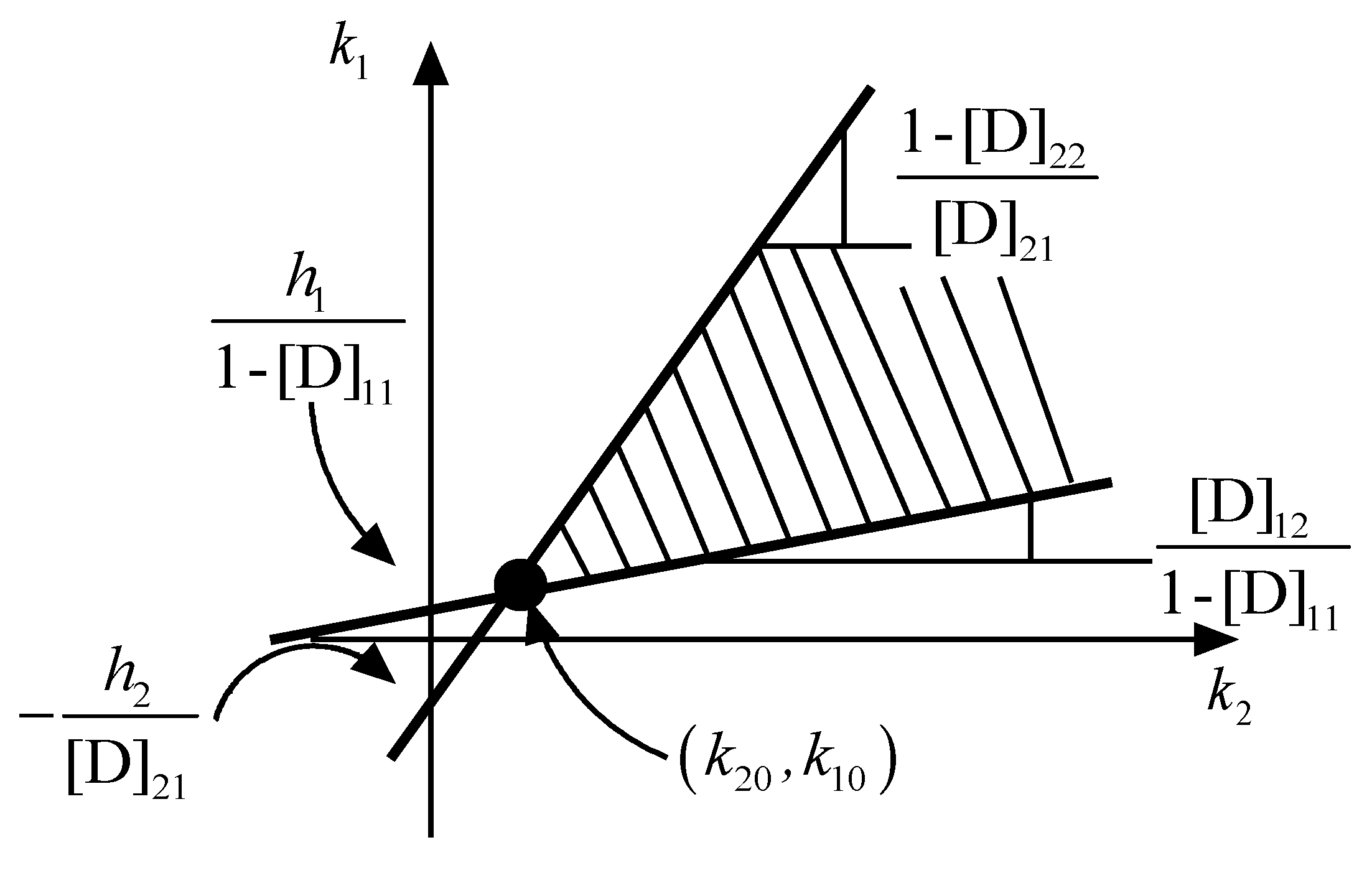
2.1. Necessary Conditions for Non-Linear MIMO Sliding Mode Control

Consider a non-linear MIMO system of the form:
x ¯ ( N ) = f ¯ ( x ¯ ) + [ B ( x ¯ ) ] u ¯
where:
x ¯ ( N ) = [ x 1 ( n 1 ) , , x m ( n m ) ] T
u ¯ = [ u 1 , , u m ] T
f ¯ ( x ¯ ) = [ f 1 ( x ¯ ) , , f m ( x ¯ ) ] T
[ B ( x ¯ ) ] = [ b 11 ( x ¯ ) b 12 ( x ¯ ) b 1 m ( x ¯ ) b m 1 ( x ¯ ) b m 2 ( x ¯ ) b m m ( x ¯ ) ]
and state vector x ¯ is defined as:
x ¯ = [ x 1 , x ˙ 1 , , x 1 ( n 1 1 ) , x 2 , x ˙ 2 , , x 2 ( n 2 1 ) , , x m , x ˙ m , , x m ( n m 1 ) ] T
Assume vector f ¯ and matrix [ B ] are not exactly known, however, their estimates, f ¯ ^ and [ B ^ ] , are known, such that the error introduced by the so-called additive uncertainties is bounded by one known function, F i , namely:
F i | f i f ^ i |
while it is possible to link [ B ^ ] and [ B ] as follows:
[ B ] = ( [ I ] + [ Δ ] ) [ B ^ ]
where [ Δ ] is an unknown matrix whose elements will be indicated with δ i j . The sliding variable vector is then defined:
s ¯ = [ s 1 s 2 s m ] T
where:
s i = ( d d t + λ i ) n i 1 x ˜ i            i = 1 , 2 , , m
In which x ˜ i is the ith tracking error. The sliding variables can be rewritten for convenience:
s ¯ = x ¯ ( N 1 ) x ¯ r ( N 1 )
where:
x ¯ r ( N 1 ) = [ x r 1 ( n 1 1 ) , x r 2 ( n 2 1 ) , , x r m ( n m 1 ) ] T
and:
x r i ( n i 1 ) = x d i ( n i 1 ) [ k = 1 n i 1 ( n i 1 k ) d n i k 1 d t n i k 1 λ i k ] x ˜ i      i = 1 , 2 , , m
where x d i is the ith state desired trajectory. The control problem can be solved by choosing the command laws as [34]:
u ¯ S M = [ B ^ ] 1 ( u ¯ ^ e q k ¯ s a t )
in which:
u ¯ ^ e q = x ¯ r ( N ) f ¯ ^
k ¯ s a t = [ Γ ] k ¯
and:
[ Γ ] = d i a g [ s a t ( s i / ϕ i ) ]      i = 1 , , m
where ϕ i is the boundary layer introduced to avoid input chattering. Please note that, in order for Equation (14) to exist, [ B ^ ] must be full-rank. The sliding condition on each s i is defined as:
1 2 d d t s i 2 η i | s i |
Which can be split into:
{ s ˙ i η i      f o r      s i 0 s ˙ i η i      f o r      s i < 0
The expression of the vector s ¯ ˙ is given by:
s ¯ ˙ = f ¯ + [ B ] [ B ^ ] 1 ( u ¯ ^ e q k ¯ s a t ) x ¯ r ( N )
Thus, Equation (20) becomes the following after a few passages:
{ ( 1 + δ i i ) k i η i + ( f i f ^ i ) + j = 1 m δ i j u ^ j e q j = 1 j i m δ i j k j s a t ( s j ϕ j )      s i > ϕ i ( 1 + δ i i ) k i η i ( f i f ^ i ) j = 1 m δ i j u ^ j e q + j = 1 j i m δ i j k j s a t ( s j ϕ j )      s i < ϕ i
These conditions can be verified by solving for k ¯ :
{ ( [ I ] [ D ] ) k ¯ ( η ¯ + F ¯ + [ D ] | x ¯ r ( N ) f ¯ ^ | ) k ¯ > 0 ¯
where the inequality is to be verified, component by component, and:
k ¯ = [ k 1 , k 2 , , k m ] T
[ D ] i j | [ Δ ] i j |
where [ D ] i j and [ Δ ] i j are the elements of [ D ] and [ Δ ] , respectevely. It follows from Equation (24) that the D-matrix is a majorant matrix of the uncertainties affecting the B-matrix. Please note that the k ¯ , F ¯ , f ¯ ^ vectors and the D-matrix are, in general, state-dependent. In order to achieve the solution of Equation (22) one has to verify that:
{ [ D ] i i < 1 λ m a x [ D ] < 1
where λ m a x [ D ] is the maximum eigenvalue of [ D ] . Indeed, it is clear from Equations (24) and (25) that matrix [ D ] cannot assume any form. In particular, it is possible to obtain Equation (22) from Equation (21) only if the elements on the diagonal of matrix [ D ] are less than 1, in addition system (22) admits a solution if matrix ( [ I ] [ D ] ) is invertible and its inverse matrix has all positive elements.
As a matter of fact, not satisfying Equation (25) implies the impossibility of sliding mode control. A detailed analysis about the origin of the second condition of Equation (25) is reported in the Appendix.

2.2. Procedure for Multiplicative Uncertainty Upper Bound Matrix Definition

In this section, a method to shape the [D] matrix is described. Referring to Equation (8), one has:
[ B ] = [ B ^ ] + [ Δ ] [ B ^ ]
Thus:
[ Δ ] = ( [ B ] [ B ^ ] ) [ B ^ ] 1
where one can define the quantity:
[ E ] i j | [ B ] i j [ B ^ ] i j |
As regards additive uncertainties, it is necessary to know the function [ E ] i j which bind the errors introduced by the multiplicative uncertainties. Remembering Equation (24), after some simple passages, the final form of [D] can be written as:
[ D ] i j = 1 | d e t [ B ^ ] | k = 1 m [ E ] i k | a d j [ B ^ ] k j |      i , j = 1 , 2 , , m
Therefore, the conditions of Equation (25) can be verified only a posteriori. It is possible to notice from Equation (29) that the entity of the error increase, [ E ] i k , caused by the multiplicative uncertainties, negatively affects the possibility of successfully designing the controller.

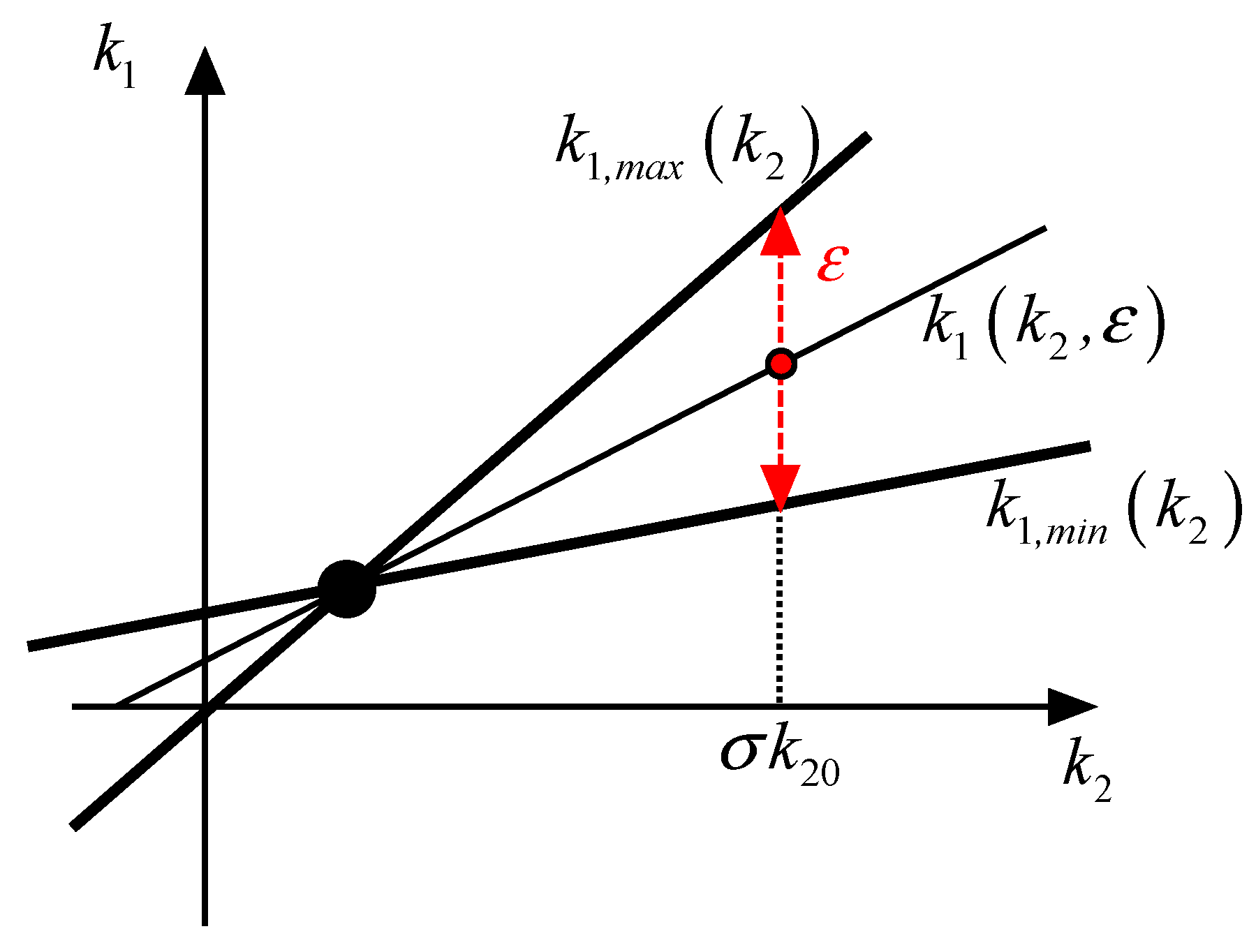
2.3. Controller Tuning Method for Systems with First-Order Channel

Consider a non-linear system of the form:
[ x ˙ 1 x ˙ 2 ] = [ f 1 ( x 1 , x 2 ) f 2 ( x 1 , x 2 ) ] + [ b 11 ( x 1 , x 2 ) b 12 ( x 1 , x 2 ) b 21 ( x 1 , x 2 ) b 22 ( x 1 , x 2 ) ] [ u 1 u 2 ]
According to Equation (14), the command laws can be written as:
u 1 S M = [ B ^ ] 11 1 ( x ˙ 1 d f ^ 1 k 1 s a t ( s 1 ϕ 1 ) ) + [ B ^ ] 12 1 ( x ˙ 2 d f ^ 2 k 2 s a t ( s 2 ϕ 2 ) )
u 2 S M = [ B ^ ] 21 1 ( x ˙ 1 d f ^ 1 k 1 s a t ( s 1 ϕ 1 ) ) + [ B ^ ] 22 1 ( x ˙ 2 d f ^ 2 k 2 s a t ( s 2 ϕ 2 ) )
where [ B ^ ] i j are the elements of [ B ^ ] .
It is possible to notice from Equations (31) and (32) that the only parameters available to modify the control laws are k 1 and k 2 . However, these parameters cannot be chosen deliberately, indeed they have to satisfy Equation (22) in order to verify Equation (18). For Equation (30) conditions, Equation (22) can be written as:
{ ( 1 [ D ] 11 ) k 1 [ D ] 12 k 2 h 1 [ D ] 21 k 1 + ( 1 [ D ] 22 ) k 2 h 2 k 1 > 0 k 2 > 0
where:
h 1 = η 1 + F 1 + [ D ] 11 | x ˙ 1 d f ^ 1 | + [ D ] 12 | x ˙ 2 d f ^ 2 |
h 2 = η 2 + F 2 + [ D ] 21 | x ˙ 1 d f ^ 1 | + [ D ] 22 | x ˙ 2 d f ^ 2 |
The solution of Equation (33) can be graphically obtained, as depicted in Figure 1, where one can observe that, in order to satisfy the sliding conditions, k 1 and k 2 can be deliberately chosen within the dashed area. One usually lets the first inequality of Equation (22) degenerate into an equation, hence the solution is given by the “cone vertex”, i.e., the point ( k 20 , k 10 ). This solution area allows one to choose the appropriate values for k 1 and k 2 (within certain boundaries) in order to obtain the desired performance from the system. In addition, k 1 and k 2 can be “moved” inside the cone depending on the state measurement, further improving the controller performance.
It is clear that both k 1 and k 2 have to be increased in order to leave the cone vertex. However, minimal “moving” of one of the two coefficients also allows a wider regulation of the other. From an operative point of view, one can approach the problem as follows. The two straight lines which individuate the cone are defined as:
{ k 1 , m a x ( k 2 ) = A k 2 + B k 1 , m i n ( k 2 ) = a k 2 + b
where:
{ A = 1 [ D ] 22 [ D ] 21 B = h 2 [ D ] 21 a = [ D ] 12 1 [ D ] 11 b = h 1 1 [ D ] 11
Hence, for a fixed value of k 2 , Equation (36) individuates the boundary values k 1 can assume. Inside this range, one can choose the desired value for k 1 by properly setting the parameter ε ∈[0; 1], according to:
k 1 ( k 2 , ε ) = [ ( A a ) ε + a ] k 2 + ( b B ) ε + b
That is, the equation of the segment depicted in red in Figure 2. Finally, k 1 and k 2 can be obtained according to the following relations:
{ k 2 = σ k 20 k 1 ( k 2 , ε ) = [ ( A a ) ε + a ] k 2 + ( b B ) ε + b
With σ > 1 . The situation is clarified by Figure 2.
Thus, regulation is achieved by properly choosing parameters σ and ε, which can also be dynamical variable functions. The performance obtained by the k 1 and k 2 motion inside the cone are compared with the ones obtained by simply setting k 10 and k 20 in the test case shown in the next section.

3. Test Case

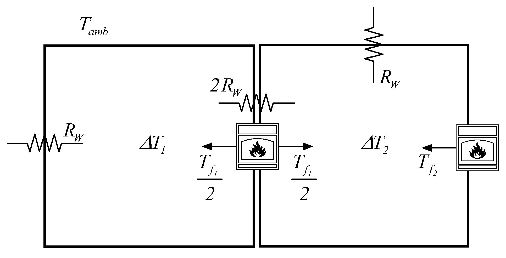
3.1. System Description and Modeling

Let us consider a system composed of two kilns, schematically represented in Figure 3.
Where Δ T 1 and Δ T 1 are the relative temperatures of the kilns with respect to ambient temperature T a m b in K, R w is the interior kiln thermal resistance in m2K/W while T f 1 and T f 2 are the thermal flows generated by the two heat sources in W. The behavior of the system can be simply described as follows:
{ T f 1 2 T f e x = c d 1 V 1 d Δ T 1 d t + S 1 R W Δ T 1 T f 1 2 + T f 2 + T f e x = c d 2 V 2 d Δ T 2 d t + S 2 R W Δ T 2
In which c is the air specific heat inside the kilns in J/(kgK), V 1 , V 2 , S 1 and S 2 are the kiln volumes and surfaces, respectively, in m3 and in m2, while d 1 and d 2 are the air densities inside the two kilns in kg/m3. In addition, the term T f e x takes into account the exchanged thermal flow between the two kilns according to:
T f e x = S 12 2 R W ( Δ T 1 Δ T 2 )
considering s 12 as the heat exchange surface in m2. Furthermore, a non-linear relation between the air density and the temperature inside each kiln is defined:
d i = T a m b Δ T i + T a m b d 0
Finally, the equations of the system written in the normal form are:
[ x ˙ 1 x ˙ 2 ] = [ ( T a m b + x 1 ) a 1 c ( A x 1 + C x 2 ) ( T a m b + x 2 ) a 2 c ( C x 1 B x 2 ) ] + [ ( T a m b + x 1 ) 2 a 1 c 0 ( T a m b + x 2 ) 2 a 2 c ( T a m b + x 2 ) a 2 c ] [ u 1 u 2 ]
where the state vector is defined as:
x ¯ = [ x 1 x 2 ] T = [ Δ T 1 Δ T 2 ] T
the inputs are:
u ¯ = [ u 1 u 2 ] T = [ T f 1 T f 2 ] T
and the output vector is:
y ¯ = [ y 1 y 2 ] T = [ x 1 x 2 ] T
In addition, some constant terms have been collected in:
a 1 = d 0 T a m b V 1 ; a 2 = d 0 T a m b V 2
A = S 12 + 2 S 1 2 R w ; B = S 12 + 2 S 2 2 R w ; C = S 12 2 R W
Hence, Equation (43) describes a MIMO non-linear system in which channels are of the 1st order. Finally, a parametric uncertainty on term c is taken into consideration, supposing its exact (unknown) value to belong to the range:
c [ c m i n     c m a x ]

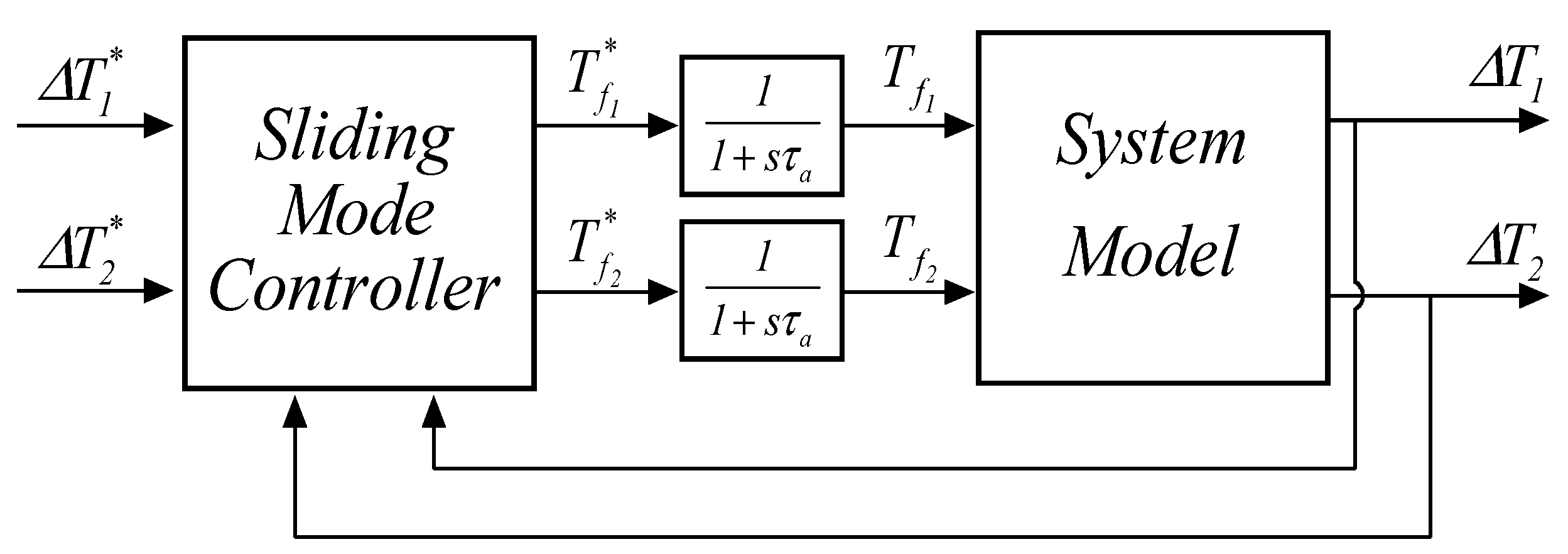
3.2. Sliding Mode Controller Design

According to the theory shown in Section 2, one can proceed to design the SM controller. The control objectives are the two relative temperatures, Δ T 1 and Δ T 2 , corresponding to the state variables of the system. Therefore, the sliding variables can be defined as:
s 1 = x 1 x 1 d
s 2 = x 2 x 2 d
In order to handle the uncertainties introduced by the not-exactly-known parameter c , an estimation of the system functions needs to be defined. In particular defining:
c ^ = c m a x + c m i n 2
one can write:
f ^ 1 = f 1 | c = c ^ = ( T a m b + x 1 ) a 1 c ^ ( A x 1 + C x 2 )
f ^ 2 = f 2 | c = c ^ = ( T a m b + x 2 ) a 2 c ^ ( C x 1 B x 2 )
b ^ 11 = b 11 | c = c ^ = ( T a m b + x 1 ) 2 a 1 c ^
b ^ 12 = b 12 | c = c ^ = 0
b ^ 21 = b 21 | c = c ^ = ( T a m b + x 2 ) 2 a 2 c ^
b ^ 22 = b 22 | c = c ^ = ( T a m b + x 2 ) a 2 c ^
and consequently:
F 1 = | 1 c m i n 1 c ^ | | T a m b + x 1 a 1 ( A x 1 + C x 2 ) |
F 2 = | 1 c m i n 1 c ^ | | T a m b + x 2 a 2 ( B x 2 + C x 1 ) |
E 11 = | 1 c m i n 1 c ^ | | T a m b + x 1 2 a 1 |
E 12 = 0
E 21 = | 1 c m i n 1 c ^ | | T a m b + x 2 2 a 2 |
E 22 = | 1 c m i n 1 c ^ | | T a m b + x 2 a 2 |
According to Equation (29), the D-matrix assumes the form:
[ D ] = [ E 11 | b ^ 11 | 0 E 21 | b ^ 22 | + E 22 | b ^ 21 | | b ^ 11 b ^ 22 | E 22 | b ^ 22 | ]
Finally, one can write the control laws as shown in Equations (31) and (32). In particular, in this case, one has:
u 1 S M = [ B ^ ] 11 1 ( x ˙ 1 d f ^ 1 k 1 s a t ( s 1 ϕ 1 ) )
u 2 S M = [ B ^ ] 21 1 ( x ˙ 1 d f ^ 1 k 1 s a t ( s 1 ϕ 1 ) ) + [ B ^ ] 22 1 ( x ˙ 2 d f ^ 2 k 2 s a t ( s 2 ϕ 2 ) )
where in the first moment, k ¯ is chosen as equal to the second side of the inequality of Equation (22):
k 10 = [ I D ] 11 1 ( η 1 + F 1 + d 11 | x ˙ 1 d f ^ 1 | )
k 20 = [ I D ] 21 1 ( η 1 + F 1 + d 21 | x ˙ 1 d f ^ 1 | ) + [ I D ] 22 1 ( η 2 + F 2 + d 22 | x ˙ 2 d f ^ 2 | )

3.3. Considerations on the Entity of Uncertainties

In this section, the effect of the error increase on the system, generated by parameter uncertainties, is investigated. The system test case is quite simple, and it is possible to make some considerations starting from the first condition of Equation (25). Looking at Equation (65) one has:
d 11 = E 11 | b ^ 11 | < 1
which, remembering Equations (55) and (61), becomes:
| 1 c m i n 1 c ^ | | ( T a m b + x 1 ) 2 a 1 | | ( T a m b + x 1 ) 2 a 1 c ^ | < 1
Finally, considering I = c m a x c m i n and after a few simple passages, one can obtain:
I c ^ < 1
This relation means that a limit on the uncertainty range extension exists, beyond which SM control is not feasible. The same analysis can be carried out for d 22 , obtaining the same result. The overall control scheme is depicted in Figure 4.
The system model and the controllers were both implemented in the MATLAB and Simulink environments, as it can be appreciated from Figure 5:

3.4. Simulation Set I

This first set of simulations aims at assessing the correct SM controller synthesis and its robustness with respect to parametric and modelling uncertainties. To this extent, together with the uncertainty on the knowledge of parameter c , two actuators (neglected in the controller synthesis) have been inserted in the system, characterized by a time constant τ a representing the delay time between the instant in which the controller orders the suitable values for T f 1 and T f 2 (labeled in Figure 4 as T f 1 * and T f 2 * ) and the one in which the two heat sources actually generate them.
The numerical values of the constant parameters used in the simulations are reported in Table 1.
As previously mentioned, the value of parameter c is not exactly known, thus it is necessary to provide its estimation and range of belonging to the SM controller. In view of what has been illustrated in the previous section, to guarantee the control feasibility, these values are chosen as:
c m i n = 772 [ J / kg K ]     ;     c m a x = 1127 [ J / kg K ]
while the value of c ^ derives from Equation (52). In this situation one has:
d 11 = d 22 = λ m a x = 0.23
Thus the conditions of Equation (25) are verified.
The simulation, as shown in Figure 6, considers a step variation in the Δ T 1 reference 10 s after the simulation start, from an initial condition of 500 °C to a steady state working point at 650 °C, while Δ T 2 reference is kept constant at 700 °C. Please remember that in this first set of simulations, k 1 = k 10 and k 2 = k 20 .
The simulation results show the correct operation of the SM controller, which is able to take the controlled variables as their references. However, from Figure 7, one can notice a non-negligible dip in the Δ T 2 profile during the transient. Figure 8 shows the time profiles of the two thermal flows coming from the two actuators.
It is interesting to investigate the system behavior with the increasing of the entity of uncertainties. By choosing a wider uncertainty range of parameter c, such that Equation (72) is violated (e.g., c m i n = 472 J/kgK; c m a x = 1427 J/kgK), the system becomes unstable, as shown in Figure 9.
Indeed, the conditions necessary for SM control feasibility are not complied with, as now:
d 11 = d 22 = λ m a x = 1.01

3.5. Simulation Set II

In this section, the controller tuning proposed in Section 3 is applied in order to improve the performance of the system. In particular, in the following attention is focused on keeping Δ T 2 as constant as possible throughout the entire transient, by dynamically regulating the terms k 1 and k 2 . For this specific test case, as D 12 = 0 , the cone assumes the shape in Figure 10.
As one can intuitively understand, an increase or decrease of k i involves a greater or smaller “strength” of the ith channel. As a consequence, in order to pursue the aforementioned goal, it is necessary to make the 2nd channel of the system “stronger” than the 1st. Therefore, during the transient, k 1 must be kept at its minimum value, while k 2 has to be dynamically increased within the dashed area in Figure 10. This means that regulation parameter ε must be zero value throughout the transient (which implies that k 1 = k 1 , m i n = k 10 ), while σ is defined on the basis of the tracking error of Δ T 2 such that, if e 2 increases, k 1 must also increase accordingly, e.g., the functional relation depicted in Figure 11.
The comparison between the performance obtained, with and without the proposed controller tuning, are presented in Figure 12, Figure 13, Figure 14, Figure 15 and Figure 16. The variable profiles obtained through the proposed tuning method are reported by red dash-dot lines, while the ones related to the conventionally tuned control system are reported by continuous blue lines.
The results of this second simulation set clearly point out the performance improvement obtained thanks to the tuning method proposed. Indeed, with an almost identical behavior of the variable Δ T 1 (Figure 12), one can notice in Figure 13 how the regulation leads to a much better profile for Δ T 2 , which does not deviate more than 5 °C from the constant reference.
Figure 14 highlights that the thermal flow injected by the first heat source is substantially the same with and without the proposed controller tuning approach, while the second is forced by the controller to produce a greater amount of heat in order to prevent the second kiln temperature from decreasing too much.
Finally, Figure 15 and Figure 16 show the regulation profiles of k 1 and k 2 compared to the limit values they can dynamically assume, highlighting that, while k 1 is always set at its minimum value, k 2 is increased during the transient to keep the corresponding temperature as constant as possible.

4. Conclusions

Some analytical remarks on the SM control theory for MIMO systems have been reported in this paper. In particular, the conditions necessary for controller feasibility on the entity of uncertainties have been thoroughly investigated. In addition, a novel controller tuning method has been proposed in order to successfully obtain the desired performance, even when the typical SM regulation parameters are not available. More precisely, it is obtained that first order SM controllers for MIMO systems can be designed as long as the so-called multiplicative uncertainties are sufficiently contained; additionally, a procedure able to exploit the uncertainty compensating terms ( k i ) both for satisfying the sliding condition and guaranteeing high controller performance is outlined. Finally, the validity of the theoretical considerations is proved through a simple test case. In order to show the effect of increasing entities of uncertainty and to illustrate the effective performance improvement obtained thanks to the proposed tuning method, a MIMO SM controller is designed and applied to the temperature regulation problem of two adjacent industrial kilns. Future developments will consider the implementation and validation of the proposed approach in a real test case or in a real time simulation environment in hardware in a loop configuration.

Author Contributions

A.P. and R.P. studied and developed the proposed tuning criteria, A.B. and M.B. provided its implementation and validation in the considered test case. A.M. supported the software implementation. I.M. and B.V. supervised the work and collaborated in the writing of the paper, together with A.M.

Funding

This research received no external funding.

Conflicts of Interest

The authors declare no conflict of interest.

Appendix A

In mathematics, the class of Z-matrices are those matrices whose off-diagonal entries are less than or equal to zero; that is, a Z-matrix A satisfies:
A = [ a i j ]    w i t h    a i j 0    f o r    a l l    i j
Definition A1.
Let A be a n × n Z-matrix. That is A = ( a i j ) where a i j 0 for all i j , 1 i , j n . Then matrix A is also a M-matrix if it can be expressed in the form:
A = s I D
where D = ( d i j ) with d i j 0 , for all 1 i , j n , s is greater than the maximum of the module of the eigenvalues of D and I is the identity matrix.
Definition A2.
Below, denotes the element-wise-order. That is, for any real matrices A, B of size m × n, we write A B if a i j b i j for all i , j .
Proposition A1.
Let D = ( d i j ) be such that d i j 0 , for all 1 i , j n with maximum eigenvalue λ m a x 1 , then I D is a M-matrix.
Proof. 
Obviously each off-diagonal term is less than or equal to 0, moreover, by choosing s = 1 we get the definition. □
Proposition A2.
If A is a M-matrix then A is inverse-positive. That is, A 1 exists and A 1 0 .
Proof. 
It can be found in Reference [39]. □

References

  1. Ubertini, S.; Facci, A.L.; Andreassi, L. Hybrid Hydrogen and Mechanical Distributed Energy Storage. Energies 2017, 10, 2035. [Google Scholar] [CrossRef]
  2. Bendato, I.; Bonfiglio, A.; Brignone, M.; Delfino, F.; Pampararo, F.; Procopio, R. A real-time Energy Management System for the integration of economical aspects and system operator requirements: Definition and validation. Renew. Energy 2017, 102, 406–416. [Google Scholar] [CrossRef]
  3. Higuchi, T.; Yokoi, Y.; Abe, T.; Sakimura, K. Design analysis of a novel synchronous generator for wind power generation. Machines 2014, 2, 202–218. [Google Scholar] [CrossRef]
  4. Bonfiglio, A.; Barillari, L.; Bendato, I.; Bracco, S.; Brignone, M.; Delfino, F.; Pampararo, F.; Procopio, R.; Robba, M.; Rossi, M. Day ahead microgrid optimization: A comparison among different models. In Proceedings of the OPT-i 2014—1st International Conference on Engineering and Applied Sciences Optimization, Kos Island, Greece, 4–6 June 2014; pp. 1153–1165. [Google Scholar]
  5. Bonfiglio, A.; Lanzarotto, D.; Marchesoni, M.; Passalacqua, M.; Procopio, R.; Repetto, M. Electrical-Loss Analysis of Power-Split Hybrid Electric Vehicles. Energies 2017, 10, 2142. [Google Scholar] [CrossRef]
  6. Passalacqua, M.; Lanzarotto, D.; Repetto, M.; Marchesoni, M. Advantages of using supercapacitors and silicon carbide on hybrid vehicle series architecture. Energies 2017, 10, 920. [Google Scholar] [CrossRef]
  7. Lanzarotto, D.; Marchesoni, M.; Passalacqua, M.; Prato, A.P.; Repetto, M. Overview of different hybrid vehicle architectures. IFAC-PapersOnLine 2018, 51, 218–222. [Google Scholar] [CrossRef]
  8. Diao, W.; Jiang, J.; Liang, H.; Zhang, C.; Jiang, Y.; Wang, L.; Mu, B. Flexible grouping for enhanced energy utilization efficiency in battery energy storage systems. Energies 2016, 9, 498. [Google Scholar] [CrossRef]
  9. Yang, X.; Wen, P.; Xue, Y.; Zheng, T.Q.; Wang, Y. Super Capacitor Energy Storage Based MMC for Energy Harvesting in Mine Hoist Application. Energies 2017, 10, 1428. [Google Scholar] [CrossRef]
  10. Bonfiglio, A.; Delfino, F.; Gonzalez-Longatt, F.; Procopio, R. Steady-state assessments of PMSGs in wind generating units. Int. J. Electr. Power Energy Syst. 2017, 90, 87–93. [Google Scholar] [CrossRef] [Green Version]
  11. Gonzalez-Longatt, F.; Bonfiglio, A.; Procopio, R.; Bogdanov, D. Practical limit of synthetic inertia in full converter wind turbine generators: Simulation approach. In Proceedings of the 2016 19th International Symposium on Electrical Apparatus and Technologies (SIELA), Bourgas, Bulgaria, 29 May–1 June 2016. [Google Scholar]
  12. Bonfiglio, A.; Delfino, F.; Invernizzi, M.; Procopio, R. Modeling and Maximum Power Point Tracking Control of Wind Generating Units Equipped with Permanent Magnet Synchronous Generators in Presence of Losses. Energies 2017, 10, 102. [Google Scholar] [CrossRef]
  13. Bemporad, A.; Borrelli, F.; Morari, M. Model predictive control based on linear programming—The explicit solution. IEEE Trans. Autom. Control 2002, 47, 1974–1985. [Google Scholar] [CrossRef]
  14. Guechi, E.-H.; Bouzoualegh, S.; Zennir, Y.; Blažič, S. MPC Control and LQ Optimal Control of A Two-Link Robot Arm: A Comparative Study. Machines 2018, 6, 37. [Google Scholar] [CrossRef]
  15. Bonfiglio, A.; Oliveri, A.; Procopio, R.; Delfino, F.; Denegri, G.B.; Invernizzi, M.; Storace, M. Improving power grids transient stability via Model Predictive Control. In Proceedings of the 2014 Power Systems Computation Conference (PSCC), Wroclaw, Poland, 18–22 August 2014. [Google Scholar]
  16. Bonfiglio, A.; Delfino, F.; Invernizzi, M.; Perfumo, A.; Procopio, R. A feedback linearization scheme for the control of synchronous generators. Electr. Power Compon. Syst. 2012, 40, 1842–1869. [Google Scholar] [CrossRef]
  17. Bonfiglio, A.; Cacciacarne, S.; Invernizzi, M.; Procopio, R.; Schiano, S.; Torre, I. Gas turbine generating units control via feedback linearization approach. Energy 2017, 121, 491–512. [Google Scholar] [CrossRef]
  18. Utkin, V.I. Sliding Modes in Control and Optimization; Springer: Berlin, Germany, 2013. [Google Scholar]
  19. Utkin, V. First Stage of VSS: People and events. In Variable Structure Systems: Towards the 21st Century; Springer: Berlin, Germany, 2002; pp. 1–32. [Google Scholar]
  20. Meng, Z.; Shao, W.; Tang, J.; Zhou, H. Sliding-mode control based on index control law for MPPT in photovoltaic systems. CES Trans. Electr. Mach. Syst. 2018, 2, 303–311. [Google Scholar] [CrossRef]
  21. Farhadi, P.; Sedaghat, M.; Sharifi, S.; Taheri, B. Power point tracking in photovoltaic systems by sliding mode control. In Proceedings of the 2017 10th International Symposium on Advanced Topics in Electrical Engineering (ATEE), Bucharest, Romania, 23–25 March 2017; pp. 781–785. [Google Scholar]
  22. Bonfiglio, A.; Cacciacarne, S.; Invernizzi, M.; Lanzarotto, D.; Palmieri, A.; Procopio, R. A Sliding Mode Control Approach for Gas Turbine Power Generators. IEEE Trans. Energy Convers. 2018. [Google Scholar] [CrossRef]
  23. Bonfiglio, A.; Invernizzi, M.; Lanzarotto, D.; Palmieri, A.; Procopio, R. Definition of a sliding mode controller accounting for a reduced order model of gas turbine set. In Proceedings of the 2017 52nd International Universities Power Engineering Conference (UPEC), Heraklion, Greece, 28–31 August 2017; pp. 1–6. [Google Scholar]
  24. Subudhi, B.; Ge, S.S. Sliding-Mode-Observer-Based Adaptive Slip Ratio Control for Electric and Hybrid Vehicles. IEEE Trans. Intell. Transp. Syst. 2012, 13, 1617–1626. [Google Scholar] [CrossRef]
  25. Liu, Y.; Shao, C. A Torque Control Scheme of Induction Motor in Hybrid Electric Vehicle. In Proceedings of the 2006 SICE-ICASE International Joint Conference, Busan, Korea, 18–21 October 2006; pp. 540–544. [Google Scholar]
  26. Emelyanov, S.; Korovin, S.; Levantovsky, L. Second order sliding modes in controlling uncertain systems. Sov. J. Comput. Syst. Sci. 1986, 24, 63–68. [Google Scholar]
  27. Levant, A. Universal single-input-single-output (SISO) sliding-mode controllers with finite-time convergence. IEEE Trans. Autom. Control 2001, 46, 1447–1451. [Google Scholar] [CrossRef]
  28. Shtessel, Y.; Edwards, C.; Fridman, L.; Levant, A. Sliding Mode Control and Observation; Springer: Berlin, Germany, 2014; Volume 10. [Google Scholar]
  29. Man, Z.; Yu, X.H. Terminal sliding mode control of MIMO linear systems. In Proceedings of the 35th IEEE Conference on Decision and Control, Kobe, Japan, 13 December 1996; pp. 4619–4624. [Google Scholar]
  30. Veselić, B.; Draženović, B.; Milosavljević, Č. Integral sliding manifold design for linear systems with additive unmatched disturbances. IEEE Trans. Autom. Control 2016, 61, 2544–2549. [Google Scholar] [CrossRef]
  31. Incremona, G.P.; Cucuzzella, M.; Ferrara, A. Adaptive suboptimal second-order sliding mode control for microgrids. Int. J. Control 2016, 89, 1849–1867. [Google Scholar] [CrossRef]
  32. Precup, R.-E.; Radac, M.-B.; Roman, R.-C.; Petriu, E.M. Model-free sliding mode control of nonlinear systems: Algorithms and experiments. Inf. Sci. 2017, 381, 176–192. [Google Scholar] [CrossRef]
  33. Komurcugil, H.; Biricik, S. Time-varying and constant switching frequency-based sliding-mode control methods for transformerless DVR employing half-bridge VSI. IEEE Trans. Ind. Electron. 2017, 64, 2570–2579. [Google Scholar] [CrossRef]
  34. Slotine, J.-J.E.; Li, W. Applied Nonlinear Control; Prentice Hall: Englewood Cliffs, NJ, USA, 1991; Volume 199. [Google Scholar]
  35. Slotine, J.-J.E. The robust control of robot manipulators. Int. J. Robot. Res. 1985, 4, 49–64. [Google Scholar] [CrossRef]
  36. Slotine, J.-J.E. Sliding controller design for non-linear systems. Int. J. Control 1984, 40, 421–434. [Google Scholar] [CrossRef]
  37. Li, D.; Slotine, J.J.E. On Sliding Control for Multi-Input Multi-Output Nonlinear Systems. In Proceedings of the 1987 American Control Conference, Minneapolis, MN, USA, 10–12 June 1987; pp. 874–879. [Google Scholar]
  38. Slotine, J.J.E.; Hong, S. Two-time Scale Sliding Control of Manipulators with Flexible Joints. In Proceedings of the 1986 American Control Conference, Seattle, WA, USA, 18–20 June 1986; pp. 805–810. [Google Scholar]
  39. Johnson, C.R.; Smith, R.L. Inverse M-matrices, II. Linear Algebra Its Appl. 2011, 435, 953–983. [Google Scholar] [CrossRef] [Green Version]
Figure 1. Graphical solution for k 1 and k 2 .
Machines 07 00010 g001
Figure 2. Regulation of k 1 and k 2 coefficients inside the cone.
Machines 07 00010 g002
Figure 3. Test case system scheme.
Machines 07 00010 g003
Figure 4. Control system scheme.
Machines 07 00010 g004
Figure 5. MATLAB and Simulink implementation.
Machines 07 00010 g005
Figure 6. Δ T 1 time profile.
Machines 07 00010 g006
Figure 7. Δ T 2 time profile.
Machines 07 00010 g007
Figure 8. Profiles of the thermal flows injected in the two kilns.
Machines 07 00010 g008
Figure 9. Unstable behavior of the system due to large uncertainties.
Machines 07 00010 g009
Figure 10. Graphical solution for k 1 and k 2 .
Machines 07 00010 g010
Figure 11. Regulation function of k 2 .
Machines 07 00010 g011
Figure 12. Performance comparison— Δ T 1 .
Machines 07 00010 g012
Figure 13. Performance comparison— Δ T 2 .
Machines 07 00010 g013
Figure 14. Performance comparison—injected thermal flows.
Machines 07 00010 g014
Figure 15. Performance comparison— k 1 profile.
Machines 07 00010 g015
Figure 16. Performance comparison— k 2 profile.
Machines 07 00010 g016
Table 1. Parameters definition.
SymbolValueSymbolValue
V 1 8 m3 V 2 15.6 m3
S 1 16 m2 S 2 25 m2
S 12 4 m2 T a m b 15 °C
d 0 1.225 kg/m3 c r e a l 1005 J/kg·K
R W 0.2 m2·K/W τ a 5 s

