Abstract
This paper presents a numerical simulation chain covering induction hardening (IH), superimposed stroke peening (StrP) as mechanical post-treatment, and a final fatigue assessment considering local material properties. Focusing on a notched round specimen as representative for engineering components, firstly, the electro-magnetic-thermal simulation of the inductive heating is performed with the software Comsol®. Secondly, the thermo-metallurgical-mechanical analysis of the hardening process is conducted by means of a user-defined interface, utilizing the software Sysweld®. Thirdly, mechanical post-treatment is numerically simulated by Abaqus®. Finally, a strain-based approach considering the evaluated local material properties is applied, which reveals sound accordance to the fatigue tests results, exhibiting a minor conservative deviation of only up to two per cent, which validates the applicability of the presented numerical fatigue approach.
1. Introduction
Induction hardening is a commonly applied post-treatment process in industrial applications, such as for gears [], crankshafts [], or railway axles []. Generally, the wear resistance [], as well as the fatigue performance [], are usually increased due to the surface-hardened layer. Hence, fatigue guidelines [] provide benefit factors for fatigue strength enhancement, due to induction hardening (IH). However, the fatigue resistance of IH parts significantly depends on the applied process parameters, as they fundamentally impact the resulting local material properties [,,]. To evaluate these local characteristics, numerous studies have validated the applicability of numerical analysis techniques to simulate the IH process [,,,,,]. In order to enhance the fatigue strength further, a previous study [] proposed that a superimposed mechanical treatment, denoted as stroke peening (StrP), of the IH surface layer is capable of elevating the local fatigue resistance. In the literature, primarily only mechanical post-treatment, such as deep rolling [] or shot peening [], has been investigated. However, a superimposed mechanical treatment of hardened surface layers is rare. Hence, this paper contributes scientifically by presenting a numerical simulation chain covering IH and the superimposed StrP manufacturing process. Finally, the numerically evaluated local material properties, such as hardness and residual stress state, are taken into account when assessing local fatigue behavior. As presented in [,] for martensitic surface layers, the local fatigue concept is applicable when properly assessing the fatigue resistance of a hardened surface layer.
Within a previous work [], the numerical simulation of the IH process and a subsequent application of a local strain-based fatigue approach was demonstrated, whereby the results fit well to the experimental data. This paper continues this preliminary study by enhancing the numerical manufacturing process chain with the superimposed StrP process. Hence, the main objective of this work is to consecutively apply available commercial CAE software packages to numerically assess the local fatigue strength of the investigated notched round specimen, incorporating the effects of the manufacturing process, including the IH and subsequent mechanical StrP post-treatment.
2. Materials and Methods
In accordance with the previous study [], the same 50CrMo4 steel was used as base material. The nominal chemical composition was specified as 0.46 to 0.54% C, maximum content of 0.40% Si, 0.50 to 0.80% Mn, 0.90 to 1.20% Cr, and 0.15 to 0.30% Mo by mass. The nominal mechanical properties were defined with 780 MPa as yield strength, and a tensile strength of approximately 1000 MPa, with an elongation of 10% at rupture. The round specimen geometry (Figure 1) exhibited a diameter of d = 30 mm and a notch, whose radius was designed to representatively cover the local stress distribution in depth, as for the investigated crankshaft in []. Details on the manufacturing of the crankshaft, the extraction of the specimens, the measurements of local properties, as well as fatigue test results for the base material, IH, and IH+StrP condition are provided in [,,].
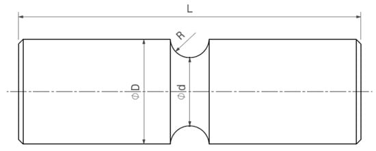
Figure 1.
Geometry of the investigated notched round specimen [].
Induction hardening consists of two parts, inductive heating and subsequent quenching. Thus, the numerical process simulation chain was separated accordingly. Firstly, the inductive heating was performed, utilizing the software Comsol® []. Thereby, a transient simulation model was built up, invoking moving mesh approach, such that the translation of the induction coils was reproduced correctly. The numerically computed position and time dependent temperature field was then transferred to Sysweld® [], wherewith the simulation of the heat-treatment process was examined. The presented IH process simulation methodology was based on a preliminary work, which is given in [,]. Beginning with the electro-magnetic-thermal simulation part, selected application studies for the utilized software are presented in [,]. Further validations of numerical and experimental results are provided in []. The main principle of the incorporated electromagnetic analysis was based on Maxwell’s equations considering the magnetic vector potential by Equation (1) []:
Thereby, j is the imaginary unit, ω is the angular frequency, κ is the electrical conductivity, ε0 is the permittivity of vacuum, εr is the relative permittivity, A is the magnetic vector potential, µ0 is the permeability in vacuum, µr is the relative permeability, B is the magnetic flux density, and Je is external current density. The resulting induced heat energy is subsequently coupled with a thermal calculation of the heat transfer according to Equation (2):
Herein, ρ is the material density, C is the heat capacity, λ is the thermal conductivity, and Qind is the induced heat energy. In addition, the heat loss due to convection and radiation was considered in the course of the numerical analysis, details see [,].
In order to properly conduct the numerical analysis, accurate material properties are of utmost importance. Thereby, selected temperature dependent values for the investigated 50CrMo4 steel are provided in []. In addition, the study in [] presents numerous material properties, not only for the electro-magnetic-thermal, but also for the subsequent thermo-metallurgical-mechanical process. Hence, the comprehensive material parameter set used in line with the preliminary works [,] was mainly gathered on the basis of []. Selected material properties of the steel 50CrMo4 are provided in Appendix A. Further information on the temperature dependent electro-magnetic material properties for the same material are given in []. The set-up of the numerical model for the inductive heating process in Comsol® is depicted in Figure 2. Due to the axial-symmetric specimen geometry, a two dimensional model was set up. Thereby, the surface layer is modeled with a fine mesh as the current density was mainly localized on the surface region based on the skin effect, which skin depth δ can be evaluated by Equation (3):
where f is the frequency of the electric current and κ is the electrical conductivity depending on the temperature-dependent electric resistance ρ(T) of the base material. In accordance to the real inductive heating process, two separate coil inductors exhibiting different current frequencies were modeled. The first coil featured a medium frequency to ensure global heating and the second coil manifested a high frequency. Thus, the electromagnetic skin depth δ was significantly reduced in respect to the higher frequency to intensify local heating in the surface layer of the specimen, as seen in Equation (3). As the coils were moving along the axis of the specimen, a moving mesh needed to be designed along this path. The ambient atmosphere was defined as air at room temperature, which was also meshed to incorporate heat loss by convection and radiation during inductive heating.
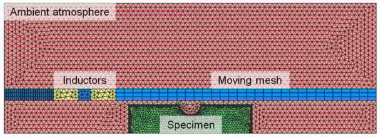
Figure 2.
Numerical model of the inductive heating process (based on []).
After simulating the inductive heating in Comsol®, the time-dependent temperature data of each node was transferred utilizing a self developed routine [] to the software package Sysweld®, in order to conduct the numerical analysis of the heat-treatment process. This self-written interface converted the temperature-time distribution for each node of the numerical model, which is the result of the simulation in Comsol®, to Sysweld®. Herein, this input data acted as the initial heating step for the thermo-metallurgic-mechanical heat-treatment analysis. As the electro-magnetic properties majorly depended on the actual temperature (see Appendix A), and not on the actual metallurgical phase of the investigated steel material, this methodology was applicable. The thermo-metallurgic-mechanical simulation in Sysweld® was performed in accordance to the models provided in the reference manual, see []. Further details on the modeling of the quenching process, in order to evaluate the local phase proportions, as well as hardness, distortion, and residual stress conditions are given in [,,,,]. Utilizing these models, the residual stress state during, and more importantly, at the end of the IH process was numerically computed, which acts, in addition to the hardness condition, as a significant input for the local fatigue analysis at the final stage of the numerical assessment methodology.
The third part of the manufacturing process simulation was the superimposed mechanical StrP process. Therefore, the resulting local material data by IH was transferred from Sysweld® to Abaqus®, in order to perform the mechanical simulation. The numerical model was set up in agreement to the experimental investigations [] incorporating a pin, which iteratively impacted the surface at the notched area of the specimen, as seen in Figure 3. The radius of the pin was comparable to the radius of the notch. The experimental results in [] highlighted that the superimposed StrP process did not majorly affect the local microstructure and hardness condition. Nevertheless, the subsequent StrP post-treatment did significantly change the residual stress state in depth, which was also the aim of the numerical analysis of the StrP simulation within this work.
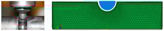
Figure 3.
Experimental StrP process of specimen [] and according to the numerical model.
Based on the preceding heat-treatment simulation in Sysweld®, the local node-dependent residual stress state, including the local IH-affected material behavior in terms of stress-strain data, acts as initial condition for the simulation of the mechanical post-treatment in Abaqus®. To properly cover hardening effects, a combined isotropic-kinematic hardening model [,] was invoked for the analysis, as this model has been shown to be applicable for the simulation of similar mechanical post-treatment processes, such as shot peening, for comparable steel materials (see []).
As a final step, the fatigue assessment based on the local strain approach was performed. Thereby, the total strain amplitude εa was calculated based on the cyclic stress-strain relationship by Ramberg-Osgood [], considering the linear-elastic stress amplitude σa, the Young’s modulus E, the cyclic strength coefficient K′, and the cyclic strain hardening exponent n′, as seen in Equation (4):
As mentioned, the numerically evaluated residual stress state due to the IH and StrP process was considered as a mean stress σm on the basis of the damage parameter PSWT by Smith, Watson, and Topper [], as seen in Equation (5):
The final fatigue assessment evaluating the number of load-cycles N until cyclic failure was performed applying the strain-life model by Manson [], Coffin [], and Basquin [] involving the fatigue strength coefficient σ‘f, the fatigue strength exponent b, the fatigue ductility coefficient ε‘f, and the fatigue ductility exponent c, as seen in Equation (6):
The material parameters K′, n′, σ′f, ε′f, b, and c, which were mandatory to perform the fatigue assessment, could be either determined based on low-cycle fatigue tests or by an estimation based on the unified material law (UML), introduced by Bäumel and Seeger []. As the original UML was focused on mild steels, an extension for high-strength steels is given in []. In both cases, the parameter evaluation mostly depends on the ultimate tensile strength (UTS). As the local Vicker’s hardness value (HV) was numerically computed by the manufacturing process simulation, the UTS could be estimated based on a suggestion in [] for steels, as seen in Equation (7):
Hence, the above presented material parameters were not constant within the fatigue analysis, but depended on the local hardness condition. As observed within the fatigue tests using the IH and IH+StrP specimens, the crack initiation origin was located either right at the very surface, or within the bulk material at the transition from the hardened surface layer to the core region. For simplification, the hardness values were determined for these two points, whereat two material parameter sets were utilized in the course of the fatigue assessment. As low-cycle fatigue test results for the IH hardened material layer were available, wherein the values were in line with the ones based on the estimation from UML, this material data set was used. As no low-cycle fatigue tests were performed for the core region, the estimation based on the local Vicker’s hardness was applied.
3. Results
3.1. Fatigue Tests
To evaluate the fatigue behavior of the researched specimens, fatigue tests under a load stress ratio of R = −1 were conducted. Figure 4 depicts the results for the IH and the IH + StrP − condition. The results were normalized with the statistically evaluated nominal fatigue strength amplitude for the base material (BM), at a number of 5e6 load-cycles and a survival probability of PS = 50%. It was shown that IH elevated the mean fatigue resistance at 5e6 load-cycles by a factor of 1.46, and IH + StrP by a factor of 1.75 compared to the BM. These results proved the beneficial effect of the post-treatment processes and the experimental values acted as basis to validate the numerical fatigue analysis. Further details of the fatigue test procedure, statistical evaluation of the fatigue data, as well as extensive fracture surface analysis, is provided in [].
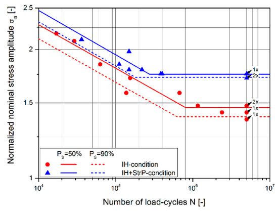
Figure 4.
Fatigue test results for induction hardening (IH) and IH + superimposed stroke peening (StrP) − condition (according to []).
3.2. Numerical Simulation
3.2.1. Electro-Magnetic-Thermal Simulation
The results of the inductive heating simulation in Comsol® are illustrated in Figure 5. At first, Figure 5a depicts the increment at which induction coil #1 started at the top end of the specimen. It is shown that a peak temperature of about 330 °C occurred at this time step. Further on, Figure 5b presents the time increment at which induction coil #2 additionally began at the top end of the specimen. Thereby, a maximum temperature of around 900 °C was computed within the model. The final condition directly after finishing the inductive heating utilizing the two coils, is depicted in Figure 5c. In this case, the peak temperature was about 840 °C and the localization of the heat input in the surface layer due to skin-effect was clearly observable. Subsequently, these time-dependent nodal temperature data were transferred to Sysweld®, utilizing a self-written script.
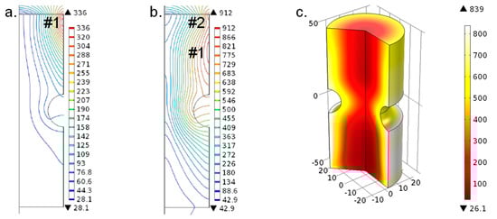
Figure 5.
Numerical results of inductive heating simulation in Comsol® (based on [,]).
3.2.2. Thermo-Metallurgical-Mechanical Simulation
After transferring the time-dependent temperature data for each node of the model from Comsol® to Sysweld®, as an initial step, the heating process was computed in Sysweld®. The results are shown Figure 6. At first, Figure 6a displays the increment at which induction coil #1 started at the top end of the specimen. It was observed that a similar peak temperature of about 330 °C occurred at this time step. Further on, Figure 6b presents the time increment at which coil #2 began, where again a similar maximum temperature of around 900 °C was computed. The final condition after finishing the heating process is depicted in Figure 6c revealing a peak temperature of about 850 °C, which was in sound accordance to the previous simulation in Comsol®. To sum up, the numerically computed temperature distribution in Sysweld® was similar to the simulation results given by Comsol®, which validated the applicability of the self-written interface.
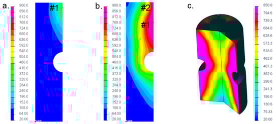
Figure 6.
Numerical results of corresponding heating processes in Sysweld® (based on [,]).
Subsequently to the heating process, the quenching of the specimen was numerically simulated in Sysweld®. Firstly, water spray cooling, and then air cooling was modeled. These cooling steps were defined in accordance to the experimental induction hardening process of the round specimen. Figure 7a demonstrates the temperature distribution during water spray cooling at the top end and Figure 7b at the notch area of the specimen. Figure 7c depicts the time increment after finishing the water spray cooling, which shows that the IH heat-treatment was effective especially at the surface-layer of the specimen. After cooling down to room temperature, the numerically computed metallurgical and mechanical results were analyzed. Figure 8a illustrates the total amount of the martensitic and Figure 8b of the ferritic/pearlitic phase. The simulated induction hardening depth fit well to a micrographical analysis of the one real specimen, see Figure 8c.
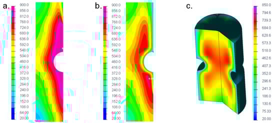
Figure 7.
Numerical results of quenching processes in Sysweld® (based on [,]).
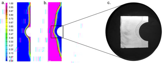
Figure 8.
Numerically computed amount of the martensitic (a) as well as ferritic/pearlitic phase (b) and comparison of induction hardening depth of a real specimen (c) (based on [,]).
A comparison of the numerically evaluated and measured Vicker’s hardness is presented in Figure 9. Therein, the values were normalized by the measured hardness of the BM. It is shown that both measurement and numerical simulation agreed well, whereby an increase of a factor of two in hardness was gained within the surface layer, due to the IH process. The effect of IH was observed up to a depth of roughly 3 mm beneath the surface at the notch root, which fit well to the numerical and experimental evaluation in Figure 8.
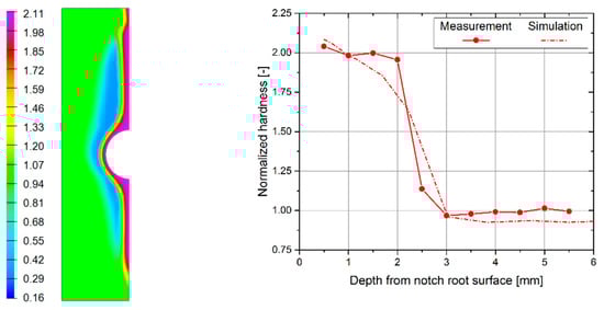
Figure 9.
Numerically computed Vicker’s hardness state and comparison of distribution in depth with measurement (based on [,]).
The finally computed axial residual stress state is shown in Figure 10. Therein, the stress values were normalized with the yield strength of the BM, which was evaluated based on quasi-static tensile tests []. The numerical results highlighted surface compressive residual stresses of about −0.55 times the yield strength of the BM. In depth, at the transition from the IH surface layer to the core material, a shift from compressive to tensile residual stresses with a normalized value of around +0.20 was maintained. Furthermore, the residual stress values were considered within the fatigue analysis. In order to simulate the third step of the manufacturing process, the mechanical StrP and the local material data was then transferred from Sysweld® to Abaqus®.
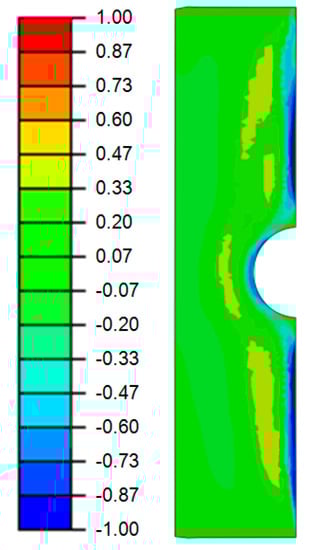
Figure 10.
Numerically computed axial residual stress distribution for IH condition.
3.2.3. Simulation of Mechanical Stroke-Peening Process
After transferring the IH process-dependent local material, as well as residual stress data from Sysweld® to Abaqus®, the superimposed StrP process as mechanical post-treatment was simulated. The axial stress results before, see Figure 11a, and during the peak compressive load, see Figure 11b, are shown as follows.
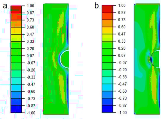
Figure 11.
Axial residual stress state before (a) and during the peak compressive load (b) of the mechanical StrP process.
During the mechanical post-treatment, it was observed that there occured comparably high compressive stress peaks below a normalized value of −1.00 within the contact area at the notch root, as seen in the black region in Figure 11b. Due to this stress state, the IH surface layer, as well as the subjacent core material, was additionally post-treated, which influenced the local residual stress state in depth. As shown by X-ray residual stress measurements in [], not only the axial but also the residual stresses in tangential direction were significantly affected by the superimposed StrP process. To cover this multiaxial residual stress state, the von Mises equivalent stress was evaluated. The final von Mises residual stress condition after the superimposed StrP is depicted in Figure 12.
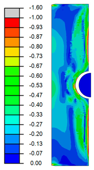
Figure 12.
Numerically computed von Mises residual stress distribution for IH+StrP condition.
The numerical simulation results maintained that, especially at the surface of the notch root the compressive residual stress state by IH was elevated due to the StrP process. Therein, a comparably high value of −1.60 times the yield strength of the BM occurred. Focusing on the core region in depth, again at the transition from the hardened surface layer to the core material, the tensile residual stress state due to IH was then shifted to compressive stress, with a value of about −0.24. This again proved the beneficial effect of the superimposed mechanical post-treatment in this case. Same as for the IH condition, these residual stress values are further on considered within the fatigue analysis.
3.3. Local Fatigue Strength Assessment
As described above, the local hardness as well as residual stress states, were utilized as input parameters for the final fatigue assessment based on the local strain-approach. Figure 13 shows a comparison of the fatigue test data and the evaluated fatigue behavior based on the local fatigue approach. It is observable that the results by the model met the average of the experimental data within the finite life region well. Focusing on the long life fatigue strength at 5e6 load-cycles, a minor conservative assessment was highlighted. However, in this case, the fatigue model fit well to the statistically evaluated S/N-curve for a survival probability of PS = 90%, as presented within the subsequent discussion. As a conservative fatigue assessment with values of PS ≥ 90% is preferentially applied, the presented fatigue model was capable of estimating the fatigue strength in this region.
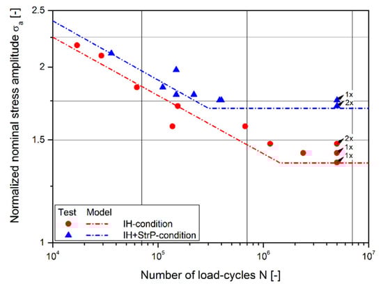
Figure 13.
Comparison of fatigue test data points to S/N-curve by fatigue model.
4. Discussion
Within this section, details of the experimental, numerical, and fatigue assessment results are given. First, Table 1 presents the statistically evaluated parameters of the S/N-curves based on the fatigue test results. As mentioned, the results were normalized with the statistically evaluated nominal fatigue strength amplitude for the base material (BM), at a number of 5e6 load-cycles and a survival probability of PS = 50%. It is shown that the normalized fatigue strength amplitude at 5e6 load-cycles was majorly elevated, by 46%, due to the IH, and by as much as 75% due to IH+StrP compared to the BM state. In addition, the number of load-cycles at the transition knee point NT were reduced, which contributed to the beneficial effect of the post-treatment processes. No significant change of the slope within the finite life region was evaluated for IH+StrP compared to IH, concluding that the StrP was most effective within the long life fatigue region at 5e6 load-cycles.

Table 1.
Comparison of the fatigue test results (evaluated at PS = 50%) for base material (BM), IH, and IH+StrP-condition [].
As shown in [], extensive residual stress investigations for the IH and IH+StrP condition were performed applying the X-ray diffraction technique. The results were taken as a basis for validating the numerical results of the manufacturing process simulation within this paper. Table 2 provides a comparison of the measured and numerically computed axial residual stresses due to IH, at the surface and in depth, at the transition from the hardened surface layer to the core material. As previously mentioned, the stress values were normalized with the yield strength of the BM, which was evaluated based on quasi-static tensile tests []. It is shown that the simulation led to a normalized residual stress at the surface of −0.55, which was only about two percent different to the measurement result and hence, validates the applicability of the numerical simulation. In depth, a tensile stress value of +0.20 was computed, which could not be compared to the measurements, as electro-chemical polishing is not applicable exceeding a depth of about two to three millimeters.
Table 2.
Comparison of axial residual stresses for IH-condition by X-ray measurements and numerical simulation.
Table 3 demonstrates a comparison of the measured and numerically computed von Mises residual stresses due to IH+StrP, at the surface and in depth, at the transition from the hardened surface layer to the core material. As described, in [], it has been revealed that the superimposed StrP process affects not only the axial, but also the residual stress state in a tangential direction. Hence, to compare this distinctive multiaxial stress state, the von Mises equivalent stress was invoked. It was shown that again the numerical manufacturing process simulation agreed well with the X-ray measurements, revealing a similar difference of only about one percent. On the contrary to the IH condition, compressive residual stresses of −0.24 were computed in depth, which proved the beneficial effect of the superimposed StrP post-treatment. However, due to the aforementioned limitations by the electro-chemical polishing process, X-ray measurements could not be performed in this depth. In addition to the previously shown local hardness condition, whereby also sound agreement between the measurements and simulation was achieved, it can be summarized that the presented simulation approach is a practical way to numerically assess the local residual stress state of induction hardened and mechanically post-treated steel components.
Table 3.
Comparison of von Mises residual stresses for IH+StrP-condition by X-ray measurements and numerical simulation.
The results of the final fatigue assessment based on the local strain approach utilizing the local hardness as well as residual stress state based on the simulation as input parameter is presented in Table 4. Therein, the long life fatigue strength amplitude at 5e6 load-cycles evaluated by the model and the fatigue tests is compared. The results of the experiments are given for a survival probability of PS = 90%, considering a conservative fatigue assessment. It is shown that in both cases IH, as well as IH+StrP condition, the fatigue model is capable of estimating the experimental results. For both conditions, the deviation of the model to the experiments was only between one and two percent, which validates the applicability of the presented numerical fatigue assessment.
Table 4.
Comparison of fatigue strength amplitude σa at 5e6 load-cycles evaluated by model and experiments (PS = 90%), for IH and IH+StrP-condition.
5. Conclusions
Based on the experimental, numerical, and fatigue assessment results within this work, the following scientific conclusions can be drawn:
- The fatigue test results reveal that induction hardening (IH) leads to an increase of 46% of the long life fatigue strength amplitude at 5e6 load-cycles compared to the base material (BM). The superimposed stroke peening (StrP) process even elevates this value again by about 20%, leading to a benefit of 75% compared to the BM.
- The numerically computed hardness state, as well as residual stress condition utilizing an electro-magnetic-thermal and thermo-metallurgical-mechanical simulation for the IH process, shows a sound agreement to the measurements. Residual stress values at the surface in an axial direction reveal a difference of only about two percent when comparing simulation and X-ray residual stress measurements.
- The simulation of the superimposed StrP process leads to similar results, whereby a minor difference of the von Mises equivalent residual stress state at the surface of only one percent between the numerical analysis and measurements is also observed.
- The final fatigue assessment highlights a sound agreement of the fatigue model, which incorporates the local hardness and residual stress state, to the experiments. Focusing on the long life fatigue strength, a minor conservative estimation with a difference of only one to two percent is shown for both IH as well as IH+StrP condition.
These conclusions basically prove the applicability of the presented numerical fatigue analysis approach for IH and IH+StrP steel components. Further work will focus on the incorporation of statistical size effects for post-treated steel layers, as shown in [] for the BM condition.
Author Contributions
Conceptualization, M.L. and R.A.; methodology, M.L. and F.G.; software, M.L. and R.A.; validation, M.L.; formal analysis, M.L. and R.A.; investigation, M.L.; writing—original draft preparation, M.L.; writing—review and editing, R.A. and F.G.; supervision, M.L. and F.G.; project administration, M.L.
Funding
This research received no external funding. Scientific support was provided in the course of the “Christian Doppler Laboratory for Manufacturing Process based Component Design”.
Conflicts of Interest
The authors declare no conflict of interest.
Appendix A
In Appendix A, selected material parameters for the investigated steel 50CrMo4 are provided, which are mainly taken from []. Table A1 shows the temperature dependence for the electrical conductivity κ, the thermal conductivity λ, and the product of the material density ρ and the heat capacity C.
Table A1.
Temperature dependence of selected material parameters for 50CrMo4 steel []
Table A1.
Temperature dependence of selected material parameters for 50CrMo4 steel []
| T [°C] | κ [MS m−1] | λ [W m−1 K−1] | ρC [J kg−1 K−1] |
|---|---|---|---|
| 0 | 4.91 | 43.1 | 451 |
| 100 | 3.90 | 42.7 | 488 |
| 200 | 3.02 | 41.7 | 528 |
| 300 | 2.40 | 40.6 | 552 |
| 400 | 1.95 | 38.9 | 619 |
| 500 | 1.60 | 37.3 | 731 |
| 600 | 1.25 | 33.7 | 762 |
| 700 | 1.05 | 31.0 | 828 |
| 800 | 1.00 | 29.5 | 836 |
| 900 | 0.97 | 28.4 | 830 |
| 1000 | 0.94 | 28.1 | 790 |
| 1100 | 0.92 | 28.8 | 732 |
| 1200 | 0.90 | 30.1 | 672 |
Table A2 provides the magnetization characteristic as B-H-curve at room temperature, which values are estimated based on [] for the same steel 50CrMo4.
Table A2.
Magnetization characteristic at room temperature for 50CrMo4 steel [].
Table A2.
Magnetization characteristic at room temperature for 50CrMo4 steel [].
| B [T] | H [A/m] |
|---|---|
| 0.08 | 500 |
| 0.32 | 1000 |
| 0.88 | 1500 |
| 1.28 | 2000 |
| 1.40 | 2500 |
| 1.48 | 3000 |
| 1.52 | 3500 |
| 1.56 | 4000 |
| 1.60 | 4500 |
| 1.64 | 5000 |
| 1.66 | 5500 |
| 1.68 | 6000 |
| 1.70 | 6500 |
| 1.72 | 7000 |
Further electro-magnetic properties as well as the temperature-dependence of the B-H-curve are presented in [] for the same steel. In addition, thermo-metallurgic-mechanical material data, such as a continuous cooling transformation (CCT) diagram, for the same base material is given in []. This material data is used for the numerical simulation of the heat-treatment in this work.
Appendix B
In Appendix B, the unified material law (UML) extended for high-strength steels as provided in [] is presented. Table A3 shows the fatigue model parameters and their estimation based on the extended UML. The parameter ψ can be evaluated as follows: ψ = 0.5{cos[π(UTS − 400)/2200] + 1}
Table A3.
Extended unified material law (UML) [].
Table A3.
Extended unified material law (UML) [].
| Parameter | Estimation |
|---|---|
| K′ | σ′f/(ε′f)n′ |
| n′ | b/c |
| σ′f | UTS(1 + ψ) |
| ε′f | 0.58ψ + 0.01 |
| b | −log(σ′f/σE)/6 |
| σE | UTS(0.32 + ψ/6) |
| c | −0.58 |
References
- Rudnev, V.; Loveless, D.; Cook, R.; Black, M. Induction Hardening of Gears: A Review. Heat Treat. Met. 2003, 30, 97–103. [Google Scholar]
- Garcia, F. Crankshaft Fillet Hardening: Challenges and Prospects. Ind. Heat. 2014, 12, 47–48. [Google Scholar]
- Fajkoš, R.; Zima, R.; Strnadel, B. Fatigue limit of induction hardened railway axles. Fatigue Fract. Eng. Mater. Struct. 2015, 38, 1255–1264. [Google Scholar] [CrossRef]
- Šofer, M.; Fajkoš, R.; Halama, R. Influence of Induction Hardening on Wear Resistance in Case of Rolling Contact. J. Mech. Eng. 2016, 66, 17–26. [Google Scholar] [CrossRef]
- Bertini, L.; Fontanari, V. Fatigue behaviour of induction hardened notched components. Int. J. Fatigue 1999, 21, 611–617. [Google Scholar] [CrossRef]
- McKelvey, S.A.; Lee, Y.-L.; Barkey, M.E. Stress-based uniaxial fatigue analysis using methods described in FKM-guideline. J. Fail. Anal. Prev. 2012, 12, 445–484. [Google Scholar] [CrossRef]
- Savaria, V.; Bridier, F.; Bocher, P. Predicting the effects of material properties gradient and residual stresses on the bending fatigue strength of induction hardened aeronautical gears. Int. J. Fatigue 2016, 85, 70–84. [Google Scholar] [CrossRef]
- Palin-Luc, T.; Coupard, D.; Dumas, C.; Bristiel, P. Simulation of multiaxial fatigue strength of steel component treated by surface induction hardening and comparison with experimental results. Int. J. Fatigue 2011, 33, 1040–1047. [Google Scholar] [CrossRef]
- Jiang, Y. Stress and fatigue analyses of an induction hardened component. Met. Mater. 1998, 4, 520–523. [Google Scholar]
- Cajner, F.; Smoljan, B.; Landek, D. Computer simulation of induction hardening. J. Mater. Process. Technol. 2004, 157, 55–60. [Google Scholar] [CrossRef]
- Ivanov, D.; Markegård, L.; Asperheim, J.I.; Kristoffersen, H. Simulation of Stress and Strain for Induction-Hardening Applications. J. Mater. Eng. Perform. 2013, 22, 3258–3268. [Google Scholar] [CrossRef]
- Fuhrmann, J.; Hömberg, D.; Uhle, M. Numerical simulation of induction hardening of steel. COMPEL 1999, 18, 482–493. [Google Scholar] [CrossRef]
- Hömberg, D.; Liu, Q.; Montalvo-Urquizo, J.; Nadolski, D.; Petzold, T.; Schmidt, A.; Schulz, A. Simulation of multi-frequency-induction-hardening including phase transitions and mechanical effects. Finite Elem. Anal. Des. 2016, 121, 86–100. [Google Scholar] [CrossRef]
- Montalvo-Urquizo, J.; Liu, Q.; Schmidt, A. Simulation of quenching involved in induction hardening including mechanical effects. Comput. Mater. Sci. 2013, 79, 639–649. [Google Scholar] [CrossRef]
- Li, H.; He, L.; Gai, K.; Jiang, R.; Zhang, C.; Li, M. Numerical simulation and experimental investigation on the induction hardening of a ball screw. Mater. Des. 2015, 87, 863–876. [Google Scholar] [CrossRef]
- Leitner, M.; Grün, F.; Tuncali, Z.; Chen, W. Fatigue and Fracture Behavior of Induction-Hardened and Superimposed Mechanically Post-treated Steel Surface Layers. J. Mater. Eng. Perform. 2018, 27, 4881–4892. [Google Scholar] [CrossRef]
- Ho, S.; Lee, Y.-L.; Kang, H.-T.; Wang, C.J. Optimization of a crankshaft rolling process for durability. Int. J. Fatigue 2009, 31, 799–808. [Google Scholar] [CrossRef]
- Bhuvaraghan, B.; Srinivasan, S.M.; Maffeo, B.; McCLain, R.D.; Potdar, Y.; Prakash, O. Shot peening simulation using discrete and finite element methods. Adv. Eng. Softw. 2010, 41, 1266–1276. [Google Scholar] [CrossRef]
- Winderlich, B. Das Konzept der lokalen Dauerfestigkeit und seine Anwendung auf martensitische Randschichten, insbesondere Laserhärtungsschichten. Materialwissenschaft und Werkstofftechnik 1990, 21, 378–389. (In German) [Google Scholar] [CrossRef]
- Kloos, K.H.; Velten, E. Berechnung der Dauerschwingfestigkeit von plasmanitrierten bauteilähnlichen Proben unter Berücksichtigung des Härte-und Eigenspannungsverlaufs. Konstruktion 1984, 36, 181–188. (In German) [Google Scholar]
- Leitner, M.; Aigner, R.; Dobberke, D. Local fatigue strength assessment of induction hardened components based on numerical manufacturing process simulation. Procedia Eng. 2018, 213, 644–650. [Google Scholar] [CrossRef]
- Leitner, M.; Vormwald, M.; Remes, H. Statistical size effect on multiaxial fatigue strength of notched steel components. Int. J. Fatigue 2017, 104, 322–333. [Google Scholar] [CrossRef]
- Leitner, M.; Tuncali, Z.; Steiner, R.; Grün, F. Multiaxial fatigue strength assessment of electroslag remelted 50CrMo4 steel crankshafts. Int. J. Fatigue 2017, 100, 159–175. [Google Scholar] [CrossRef]
- Pryor, R.W. Multiphysics Modeling Using COMSOL. A First Principles Approach; Jones and Bartlett Publication: Boston, MA, USA, 2011. [Google Scholar]
- Pont, D.; Guichard, T. Sysweld®: Welding and Heat Treatment Modelling Tools. In Computational Mechanics’95; Springer: Berlin, Germany, 1995; pp. 248–253. [Google Scholar]
- Aigner, R. Aufbau Einer Numerischen Simulationskette für Induktionsgehärtete Randschichten. Master’s Thesis, Montanuniversität Leoben, Leoben, Austria, 2016. (In German). [Google Scholar]
- Istardi, D.; Triwinarko, A. Induction heating process design using comsol multiphysics software. Telecommun. Comput. Electron. Control 2013, 9, 327–334. [Google Scholar] [CrossRef]
- Ocilka, M.; Kovác, D. Simulation model of induction heating in Comsol Multiphysics. AEI 2015, 15, 29–33. [Google Scholar] [CrossRef]
- Kennedy, M.; Shahid, A.; Jon Arne, B.; Ragnhild, E.A. Analytical and Experimental Validation of Electromagnetic Simulations Using COMSOL®, re Inductance, Induction Heating and Magnetic Fields. In Proceedings of the COMSOL Users Conference, Stuttgart, Germany, 26–28 October 2011. [Google Scholar]
- Rudnev, V.; Loveless, D.; Cook, R.L. Handbook of Induction Heating; CRC Press: Boca Raton, FL, USA, 2017. [Google Scholar]
- Comsol, A.B. COMSOL Reference Manual, version 5.2a; COMSOL Inc.: Burlington, MA, USA, 2016. [Google Scholar]
- Barglik, J.; Smalcerz, A.; Przylucki, R.; Doležel, I. 3D modeling of induction hardening of gear wheels. J. Comput. Appl. Math. 2014, 270, 231–240. [Google Scholar] [CrossRef]
- Fisk, M.; Lindgren, L.-E.; Datchary, W.; Deshmukh, V. Modelling of induction hardening in low alloy steels. Finite Elem. Anal. Des. 2018, 144, 61–75. [Google Scholar] [CrossRef]
- ESI Group. SYSWELD Reference Manual; ESI Group: Paris, France, 2009. [Google Scholar]
- Liščić, B. Quenching Theory and Technology, 2nd ed.; CRC Press: Boca Raton, FL, USA, 2010. [Google Scholar]
- Wolff, M.; Acht, C.; Böhm, M.; Meier, S. Modelling of carbon diffusion and ferritic phase transformations in an unalloyed hypoeutectoid steel. Arch. Mech. 2007, 59, 435–466. [Google Scholar]
- Magnabosco, I.; Ferro, P.; Tiziani, A.; Bonollo, F. Induction heat treatment of a ISO C45 steel bar: Experimental and numerical analysis. Comput. Mater. Sci. 2006, 35, 98–106. [Google Scholar] [CrossRef]
- Jung, M.; Kang, M.; Lee, Y.-K. Finite-element simulation of quenching incorporating improved transformation kinetics in a plain medium-carbon steel. Acta Mater. 2012, 60, 525–536. [Google Scholar] [CrossRef]
- Hibbit, D.; Karlsson, B.; Sorenson, P. ABAQUS Reference Manual 6.7; ABAQUS Inc.: Pawtucket, RI, USA, 2005. [Google Scholar]
- Chaboche, J.-L. Constitutive equations for cyclic plasticity and cyclic viscoplasticity. Int. J. Plast. 1989, 5, 247–302. [Google Scholar] [CrossRef]
- Klemenz, M.; Schulze, V.; Rohr, I.; Löhe, D. Application of the FEM for the prediction of the surface layer characteristics after shot peening. J. Mater. Process. Technol. 2009, 209, 4093–4102. [Google Scholar] [CrossRef]
- Ramberg, W.; Osgood, W.R. Description of Stress-Strain Curves by Three Parameters; National Advisory Committee for Aeronautics: Washington, DC, USA, 1943. [Google Scholar]
- Smith, K.N.; Watson, P.; Topper, T. Stress-Strain function for fatigue of metals. J. Mater. 1970, 5, 767–778. [Google Scholar]
- Manson, S.S. Fatigue: A complex subject—Some simple approximations. Exp. Mech. 1965, 5, 193–226. [Google Scholar] [CrossRef]
- Coffin, L.F. A study of the effect of cyclic thermal stresses on a ductile material. Trans. ASME 1954, 76, 931–950. [Google Scholar]
- Basquin, O.H. The exponential law of endurance tests. Am. Soc. Test. Mater. Proc. 1910, 10, 625–630. [Google Scholar]
- Baumel, A., Jr.; Seeger, T. Materials Data for Cyclic Loading. Supplement 1; Elsevier Science Publishers: Amsterdam, The Netherlands, 1990. [Google Scholar]
- Korkmaz, S. Extension of the Uniform Material Law for High Strength Steels. Master’s Thesis, Bauhaus University, Weimar, Germany, 2008. [Google Scholar]
- Pavlina, E.J.; van Tyne, C.J. Correlation of Yield Strength and Tensile Strength with Hardness for Steels. J. Mater. Eng. Perform. 2008, 17, 888–893. [Google Scholar] [CrossRef]
© 2019 by the authors. Licensee MDPI, Basel, Switzerland. This article is an open access article distributed under the terms and conditions of the Creative Commons Attribution (CC BY) license (http://creativecommons.org/licenses/by/4.0/).