Abstract
The purpose of this paper is to choose a new topology for bearingless flux-switching slice motors, regarding the number of stator and rotor poles, with a combined winding set. Additionally, the selected motor topology is optimized with finite element method (FEM) simulations to improve the performance. Bearingless slice drives feature a magnetically-suspended rotor disk passively stabilized by reluctance forces due to a permanent magnet (PM) bias flux in the air gap and actively controlled by the generation of radial bearing forces and motor torque. Usage of the combined winding set, where each phase generates both motor torque and suspension forces, opens the opportunity for a new topology. The topology choice and optimization are based on FEM simulations of several motor optimization criteria, as the passive axial, tilting and radial stiffness values and the active torque and bearing forces, which are simulated regarding the motor height and specific stator and rotor parameters. Saturation, cogging torque and cogging forces are also analyzed. The 3D FEM program ANSYS Maxwell 2015 was used. The results led to an optimized bearingless flux-switching motor topology with six new stator segments and seven rotor poles. By optimizing the geometry, a considerable improvement of performance was reached. This geometry optimization is a base for a future prototype model.
1. Introduction
1.1. History and Description of the Bearingless Motor
At the beginning of the 20th Century, the idea of magnetic levitation was presented, which was followed by the development of concepts to stabilize a rotor [1,2,3,4,5]. This research led to the development of the first bearingless motor. The bearingless motor concept started developing and spreading in universities and industry world-wide around the year 1990, especially in Japan and Switzerland [1,2,3,4,5]. The bearingless motor is a magnetically-levitated drive generating both torque and bearing force in one single device.
1.2. Bearingless Permanent Magnetic Flux-Switching Slice Motor
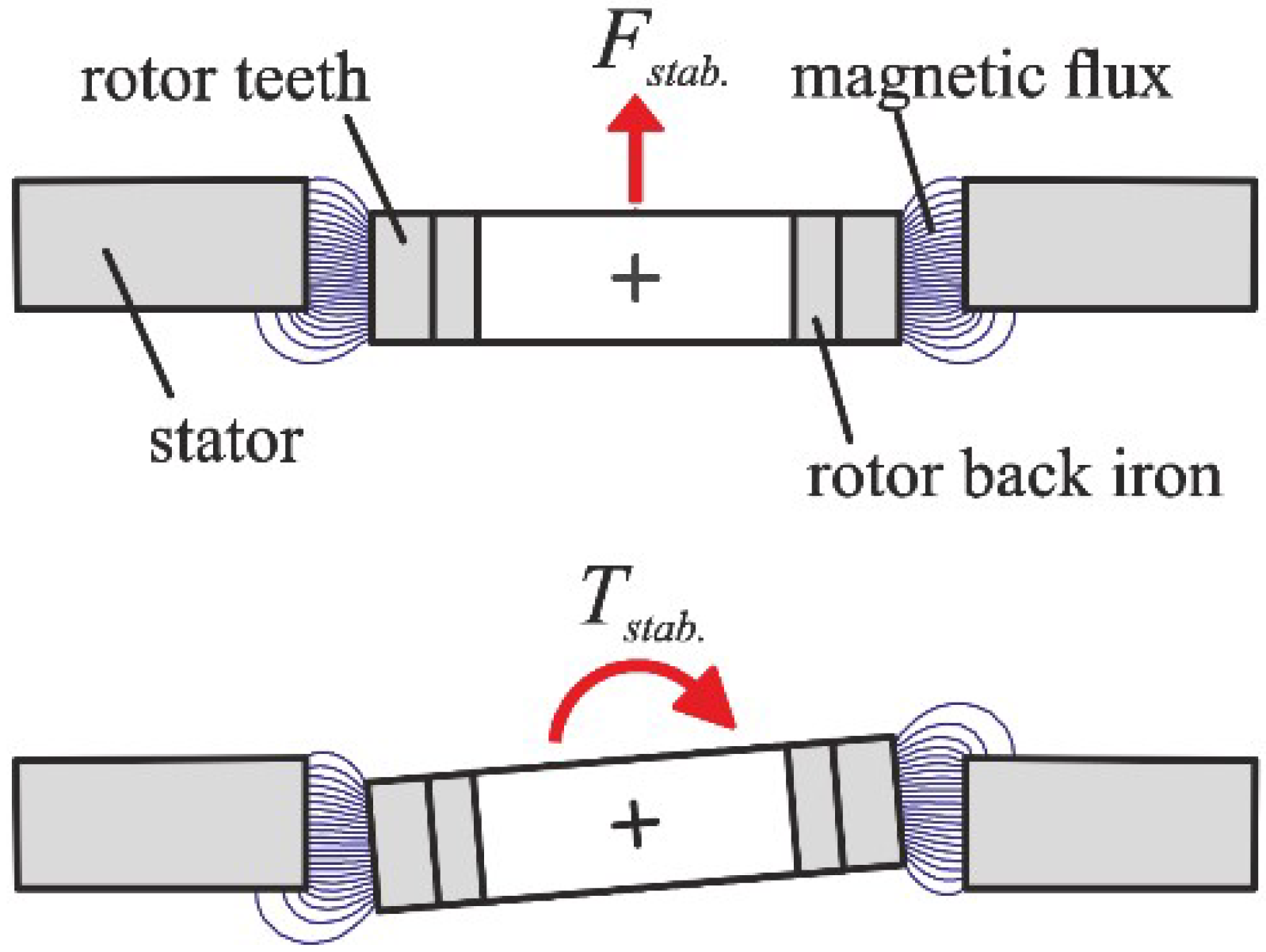
A further step of simplification in the bearingless motor setup was achieved by using a slice motor [6], which is also used in this research. “Slice” implies that the rotor is disk-shaped; hence, the length of the rotor is much smaller compared to its diameter. Thus, the axial (z-direction) and tilting directions around the x- and y-directions of this rotor can be passively stabilized in the presence of a magnetic air-gap field [6]. In this case, stabilizing reluctance forces are created. This passive reluctance stabilization is illustrated in Figure 1.
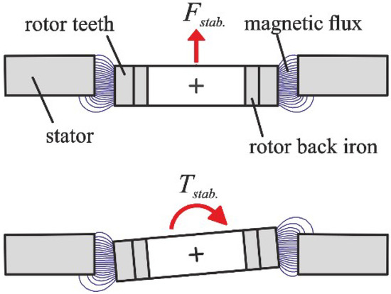
Figure 1.
Passive stabilization for the axial (top) and tilting (bottom) deflection [7].
Since, with passive stabilization, three degrees of freedom are stabilized, active regulation must be provided for the radial positions (x- and y-directions) and the rotor angle [8]. This paper deals with a bearingless flux-switching slice motor. The principle of “flux-switching” is shown in Figure 2. A salient rotor is moving along stator poles, which are creating an alternating flux in the iron of the stator teeth. Each stator tooth holds a coil; subsequently, back electromotive force (EMF) is induced in the windings [9].
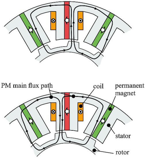
Figure 2.
PM flux path depending on the rotor angle [9].
Applications of bearingless drives are pumps [10,11] in the semiconductor and medical industry, high temperature and high-speed applications and in disposable devices where the rotor has to be removed. Since the FSPM features a magnet-free rotor, rotor manufacturing costs are also lower [12,13].
1.3. New Topology with Combined Windings
Bearing force generation and torque characteristics strongly depend on the winding system. A rotating field created by a winding system featuring the same number of pole pairs as the PM field generates torque and field weakening. On the other hand, a rotating stator field with a pole pair number differing by one from the PM field generates radial bearing forces [1]. Hence, bearingless slice motors often use two different kinds of winding sets. This then is called a separated winding set, where one phase creates only motor torque, while other phases create only suspension forces. Moreover, two connected coils are needed for one phase. In that concept, both winding sets and therefore motor torque and bearing forces are completely separated (decoupled) and can be relatively easily controlled. The disadvantages of this setup are worse efficiency and manufacturability [11]. Another possibility is to use a winding set which is called a combined winding set, which was proposed by [14]. This winding set is also used in this research. In this concept, each phase generates both motor torque and suspension forces. The advantage of this setup is the usage of one coil per phase, which is an improvementin manufacturability with reduced copper loss in the windings. Complexity is shifted to control. Nonlinear schemes and control methods have to be implemented to decouple motor torque and bearing forces properly for a bearingless motor operation [15].
The goal is to determine a new topology for operation, which uses a combined winding set. Secondly, the new topology will be optimized by FEM for improved performance. In order to simplify the understanding, the readers will first be introduced to the operating principle of the bearingless drive. Before the simulation results, geometrical parameters of the FSPM will be presented followed by the simulation explanation.
2. Setup
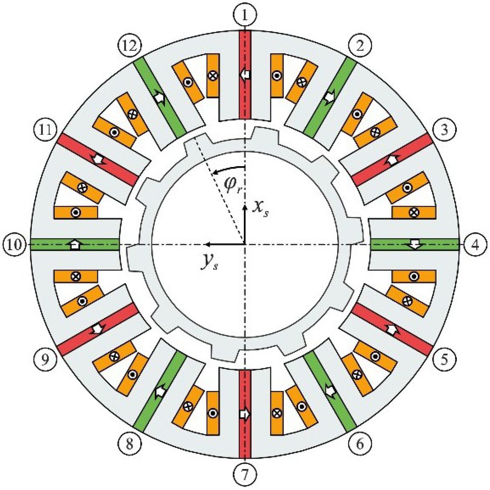
An existing bearingless FSPM with 12 stator segments and 10 rotor poles is shown in Figure 3 [16]. The number of stator segments is described by the parameter , while the rotor pole number is . and are changed in Section 4. However, around each stator tooth, one coil is wound. Active force and torque generation is possible through opposing coils (like 1 and 7, 2 and ) when properly energized. The main coil parameter is the magneto-motive force (MMF) of each coil. The MMF is changed from 0–1000 Aturns; 0 Aturns is used to calculate the passive stiffness, while 1000 Aturns is used to determine the active bearing force and motor torque.
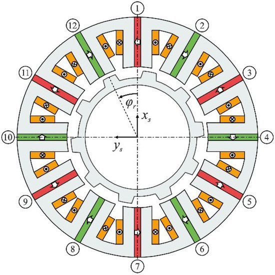
Figure 3.
Cross-section of a bearingless flux-switching slice motor with twelve stator teeth and ten rotor poles [16].
2.1. Stator Teeth Geometry
The circumferential length of one stator segment is calculated by:
where the outer diameter of the rotor is given by and the air gap length is defined by .
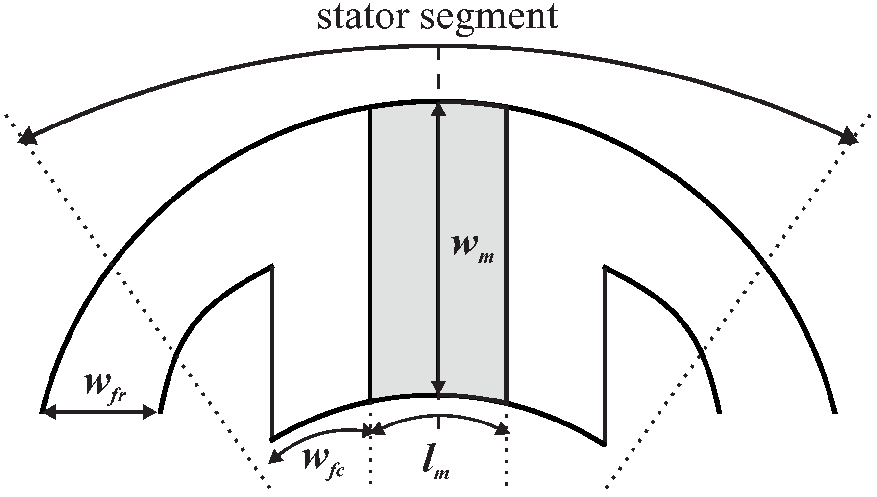
The stator teeth are composed of two iron parts and a permanent magnet in between. Every second, the PM has the opposite polarization. The circumferential length of the iron part of the stator tooth is defined by parameter . The PM’s radial length is , while its length is defined by the parameter . The thickness of the stator segment back yoke is defined by the parameter and controlled by parameter by:
These stator parameters are shown in Figure 4.
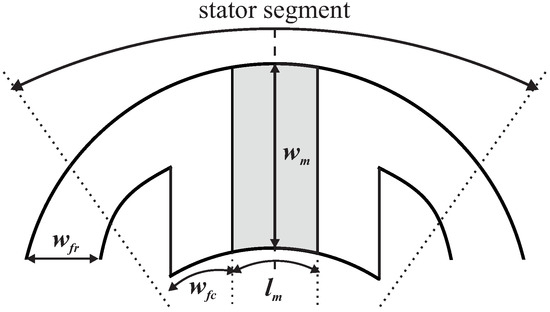
Figure 4.
Cross-section of a stator segment with the corresponding parameters.
2.2. Rotor Geometry
The rotor is disk-shaped with salient poles. Apart from the outer diameter of the rotor (), the inner diameter of the rotor is called and calculated by:
where defines radial height of the rotor teeth.
Furthermore, it is important to mention the three rotor parameters that are optimized. The first one is , which influences the parameter , representing the outer circumferential length of the stator teeth defined as:
The second optimization parameter is , which changes the radial length of the rotor teeth by:
The last optimization parameter is , which changes the inner circumferential length of the rotor tooth along with the parameter , representing the rotor pole angle. The rotor parameters are shown in Figure 5.
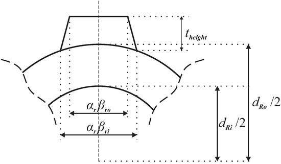
Figure 5.
Cross-section of a rotor pole with corresponding parameters.
2.3. Motor Height
The motor height in the z-direction is changed by the parameter . With the need to add or remove the stator or rotor height on constant parameter , the two following parameters are defined: changes the stator height, while the parameter sets the additional rotor height.
2.4. Air Gap
Some industrial applications demand motors with an increased air gap. A larger air gap simplifies the hermetic separation of the stator and rotor, but leads to reduced overall performance [16]. With smaller air gaps, higher torque and bearing forces are generated, but the radial destabilizing forces are also increasing. In this research, the air gap length is set to 3 mm due to the necessity of a process chamber wall in the air gap.
2.5. Magnetic Saturation
Magnetic saturation leads to nonlinear motor behavior. Magnetic saturation is a characteristic of ferromagnetic materials where each material reaches saturation at different values. Since the force and motor torque of the FSPM are not decoupled any longer if the stator or rotor iron is magnetically saturated, magnetic flux density in FSPM should not exceed 1.5 T. In the simulations for passive stiffness without current through the coils, the risk of saturation is low, but in the simulations for active bearing forces and motor torque, it is necessary to check for iron saturation. Figure 6 shows one part of the FSPM with its magnetic flux density where different colors present the value of magnetic saturation. Red-colored parts are saturated as they feature over 1.5 T of magnetic flux density. The saturation can be avoided in two ways:
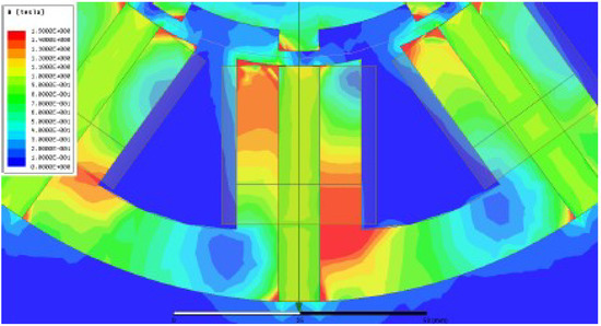
Figure 6.
Part of the FSPM with its magnetic flux density.
- use lower coil currents;
- change the back yoke of the stator iron (parameter ) to increase the cross-sections of the back yoke.
3. Simulations
A parametric geometric model and a magnetostatic simulation setup are implemented in ANSYS Maxwell 3D FEM program. The results of the topology choice and optimization based on the simulations in this program are described in the next sections.
3.1. Simulation Parameters
In order to move or rotate the rotor in the simulations, the parameters in Table 1 are used.

Table 1.
Simulation parameters.
3.2. Motor Optimization Criteria
The motor optimization criteria are the passive stiffness values and the active torque and force generation. The topology selection and further optimization of the chosen motor topology are based on the results of the following motor optimization criteria. It is aimed to have high motor torque and suspension forces with good passive stabilization in the axial and tilting direction [16].
3.2.1. Passive Stiffness Values
Reluctant forces are exerted on the deflected rotor due to the bias flux of the PMs in the air gap. Three degrees of freedom are stabilized by three passive forces. These passive stiffnesses are the following:
- Axial stiffness ( in N/mm) is defined as stabilizing force per axial deflection of the rotor in the z-direction. In the FEM simulations, the rotor is displaced 1 mm from its center position. The value of the axial stiffness is negative and thus stabilizing. Hence, it is desirable to achieve high absolute values;
- Tilting stiffness ( and in Nm/deg) is defined as the stabilizing motor torque per degree due to PM reluctance forces when the rotor is tilted around the x- and y-axis. In the FEM simulations, the rotor is tilted 1 deg around the x- and y-axis, respectively, and the value of the tilting stiffness is negative, indicating stabilizing behavior. Again, higher absolute values are preferable;
- Radial stiffness ( and in N/mm) is defined as destabilizing radial force per deflection on the rotor pulling the rotor and the stator together. Active bearing forces have to be generated in order to overcome these forces. The radial reluctance forces are different from the other described passive forces as they destabilize the system; thus, it is desired that the radial stiffness features smaller absolute values. In simulations, the rotor is radially displaced 1 mm in the x- and y-directions to compute the radial stiffness values.
3.2.2. Active Suspension Forces and Drive Torque
The radial rotor position is achieved by actively stabilized bearing forces. These forces and the motor torque are generated by the stator currents. Due to the used control scheme, bearing forces and motor torque must have a linear dependency on the current; therefore, saturation is not permissible. Additionally, no square force to current dependency should be present [16]. In the FEM simulation for active bearing forces and motor torque, a constant magneto-motive force is fed to one coil, and the rotor angle is varied. As one period of the rotor angle is dependent on the number of rotor poles, the simulated rotor angle is different for certain topologies. The active single-phase bearing forces, and , and the single-phase motor torque feature a sinusoidal shape and are shown in Figure 7.
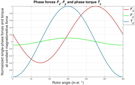
Figure 7.
Part of the FSPM with its magnetic flux density.
4. Topology Choice
The first goal of this paper is to determine the most suitable topology for an FPSM. More precisely, as the “topology”, a certain number of stator segments and rotor poles are considered. The parameters and are chosen based on the simulation results regarding the motor optimization criteria. Some parameters of the FPSM are defined to be constant. These static parameters are the air gap, the axial motor height, the rotor diameter and the stator and rotor width parameters. They are summarized in Table 2 with their respective values.
Table 2.
Constant parameters in the topology choice and for optimization.
4.1. Results
The obtained FEM results are shown in Table 3, presenting the bearing forces and motor torque. The most important criteria for topology selection were:
Table 3.
Simulation results for different topologies.
- The cogging forces are the forces exerted on the rotor only by the PM field ( (0 At) and (0 At) in Table 3) and should be small and exceeded by the active motor active forces with 1000 At in one coil.
Previous research showed that cogging torque and cogging forces depend on the magnet shapes, dimensions, locations, magnetization patterns and slot/pole combination [17]. This holds also true in this research. Additionally, axial stiffness, tilting stiffness, active forces and motor torque should be as high as possible, while the radial stiffness should be as small as possible.
4.2. Favorable Topologies
First, topologies with different parameters and are separated into feasible and unfeasible topologies in Table 4 based on the two most important rules considering the cogging forces and cogging torque described before.
Table 4.
Topologies separated based on the results of Table 3.
Unfeasible topologies in Table 4 feature either high cogging torque or high cogging x- and y-forces (characterized in Table 3). Hence, they become excluded from further considerations regarding the axial, radial and tilting stiffness. The topology S6R7 seems to be the most promising (Table 3); since this topology has acceptable values of cogging forces and cogging torque, its motor torque (1000 At) is the highest and its magnetic flux density the lower than the other simulated topologies with higher values of parameter (8 and 10).
5. Optimization
The optimization process is stepwise by changing one stator or rotor parameter after the other. Thus, the optimization is divided into four steps, which are presented in this section. The variable geometry parameters are grouped as follows:
- Motor height , optimization of the parameters that define the motor height (in the axial z-direction), for both the stator and the rotor: and ;
- Stator geometry, optimization of the stator parameters: and ;
- Rotor geometry, optimization of the rotor parameters: and .
5.1. FEM Simulations and Optimization Results
- Step 1:
- Motor height.
The first parameter that was optimized is the axial height of the stator and the rotor, which feature the same axial height at first. The values of the other parameters are given in Table 2. The simulation range and step size are presented in Table 5.
Table 5.
Parameter simulation information.
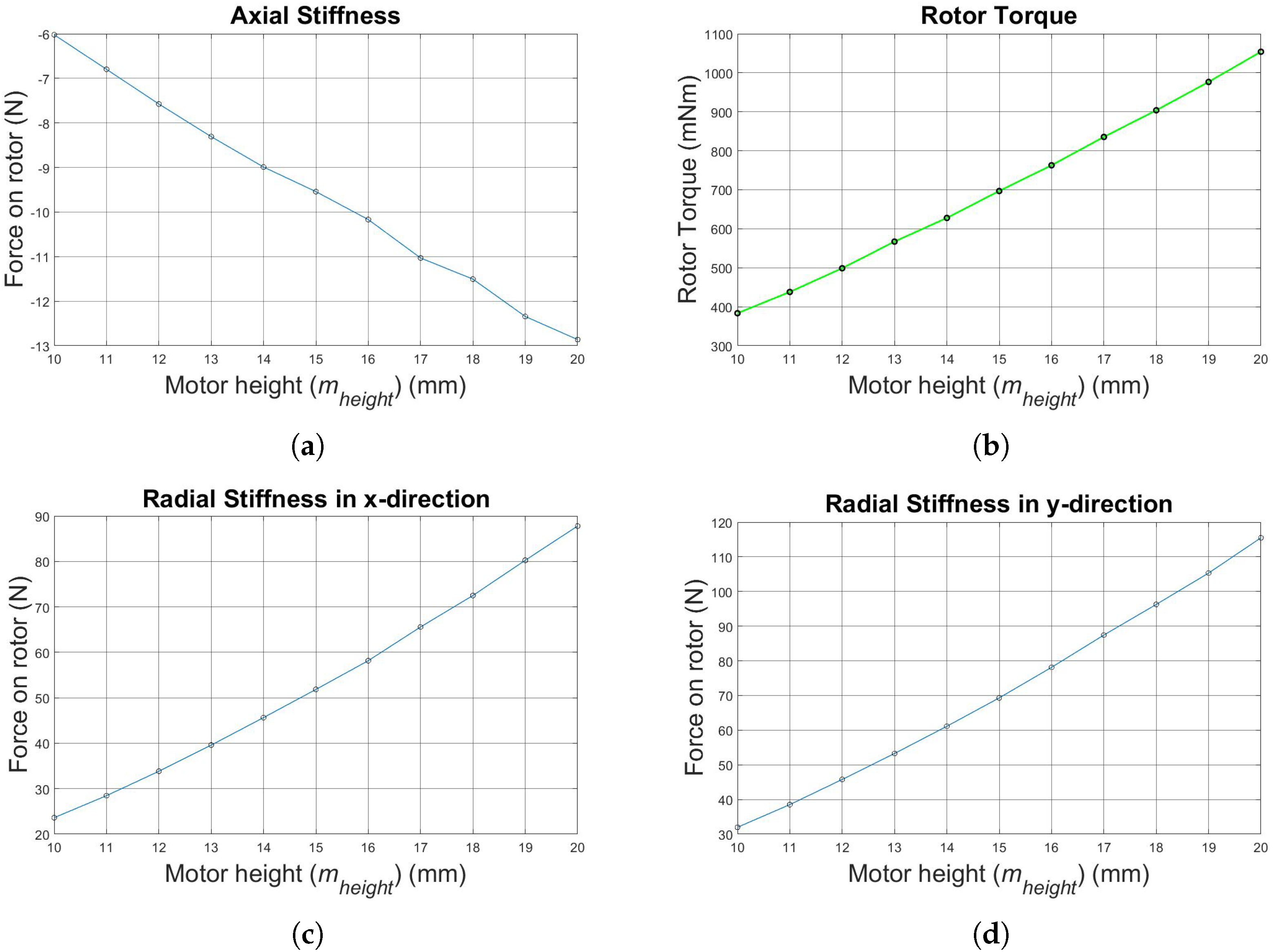
The most important results, which are shown in Figure 8e,f, are the characteristics of the tilting stiffness values in the x- and y-direction, where higher absolute values are preferable. This leads to an increase of 14% in the x-direction and 23% in the y-direction tilting stiffness. Additionally, higher absolute values regard the axial stiffness and the active bearing forces and torque that are reached. Parameter is set to 14 mm (instead of 10 mm).
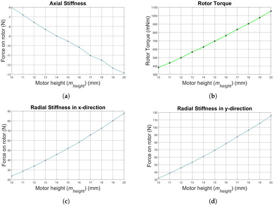
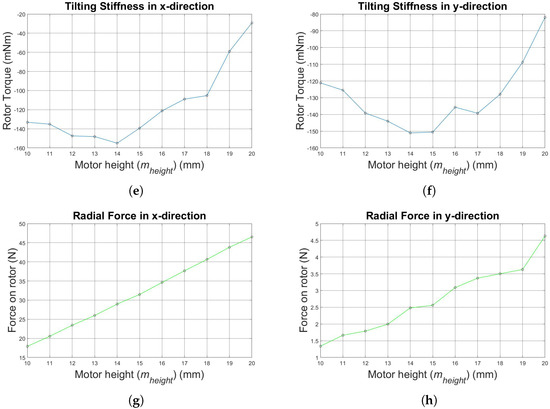
Figure 8.
Simulation results for increasing motor height: (a) axial stiffness, (b) rotor torque, (c) radial stiffness in the x-direction, (d) radial stiffness in the y-direction, (e) tilting stiffness in the x-direction, (f) tilting stiffness in the y-direction, (g) radial bearing force in the x-direction and (h) radial bearing force in the y-direction.
- Step 2:
- Stator and rotor height.
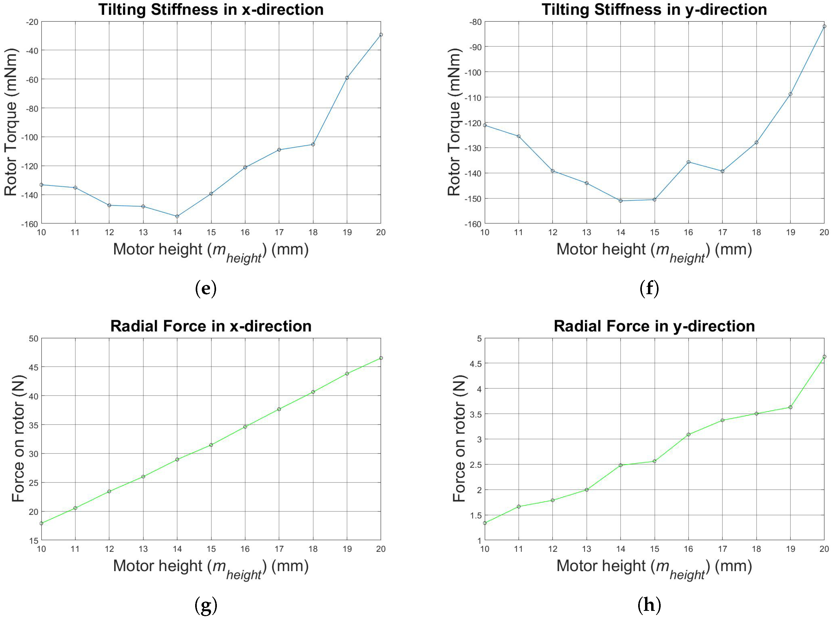
In the next step, different stator and rotor heights (in the z-direction) are reached. The reference simulations for the tilting stiffness are shown in Figure 9a for decreasing rotor height and in Figure 9b for increasing stator height.
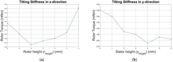
Figure 9.
(a) Tilting stiffness in the x-direction with decreasing rotor height; (b) tilting stiffness in the y-direction with increasing stator height.
Since the highest absolute value for the tilting stiffness is given for a constant stator height equal to 14 mm and a decreased rotor height at 10 mm (an increase of 16%) and a constant rotor height equal to 14 mm and an increased stator height at 18 mm (an increase of 37%), further comparisons and simulations are conducted regarding these two setups. The simulation results of those two setups are shown in Table 6. The second variant with increased stator height is selected for further consideration.
Table 6.
Simulation results for decreased rotor and increased stator.
- Step 3:
- Stator geometry.
The circumferential length of the iron part of the stator tooth () is computed by parameter given by:
where the parameter M is defined as the circumferential length of the stator segment divided by the sum of the stator segment parameters as defined in:
The PM’s length () is computed by parameter :
The space between two stator teeth is set by the parameter . These three stator parameters and affect the motor performance. As mentioned before, these parameters are varied one after the other. The simulation ranges and step size are given in Table 7.
Table 7.
Simulation information of the stator parameters.
First, the parameter is optimized. The characteristics for rotor torque shown in Figure 10 and tilting stiffness shown in Figure 11 are considered.
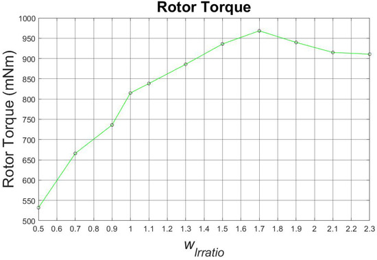
Figure 10.
Rotor torque over the parameter
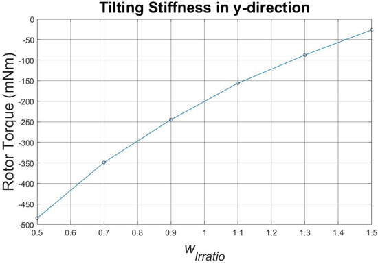
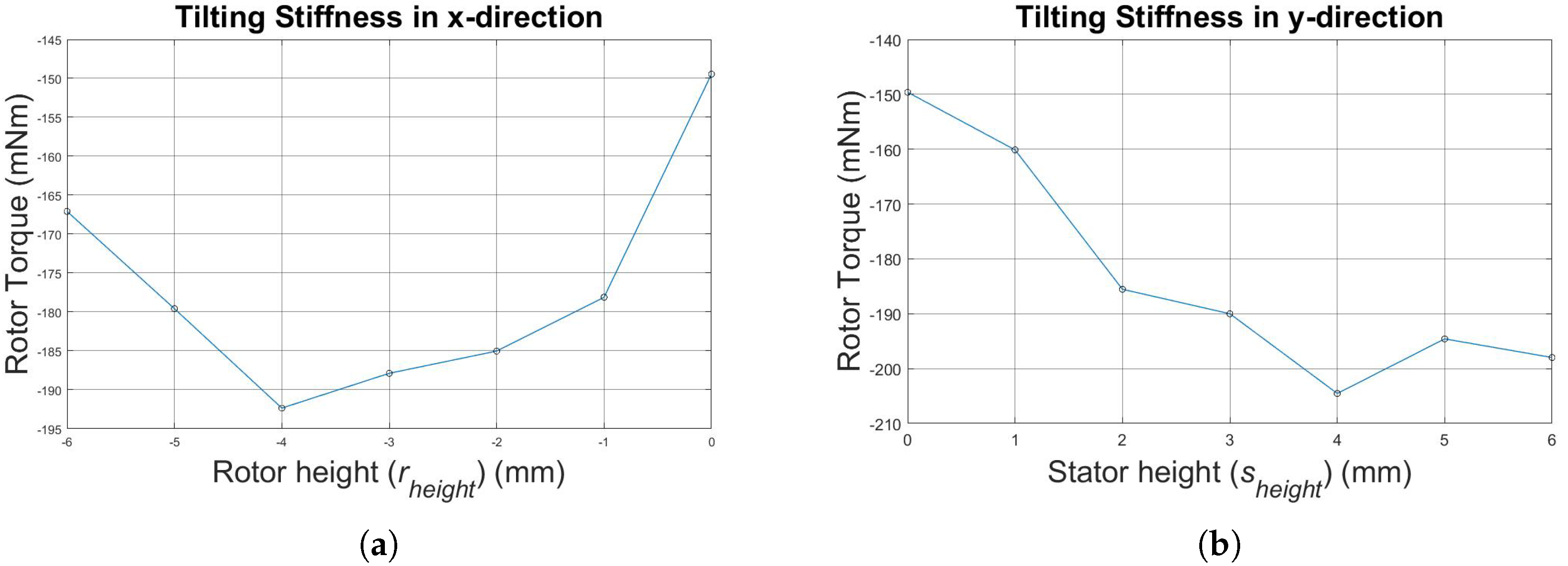
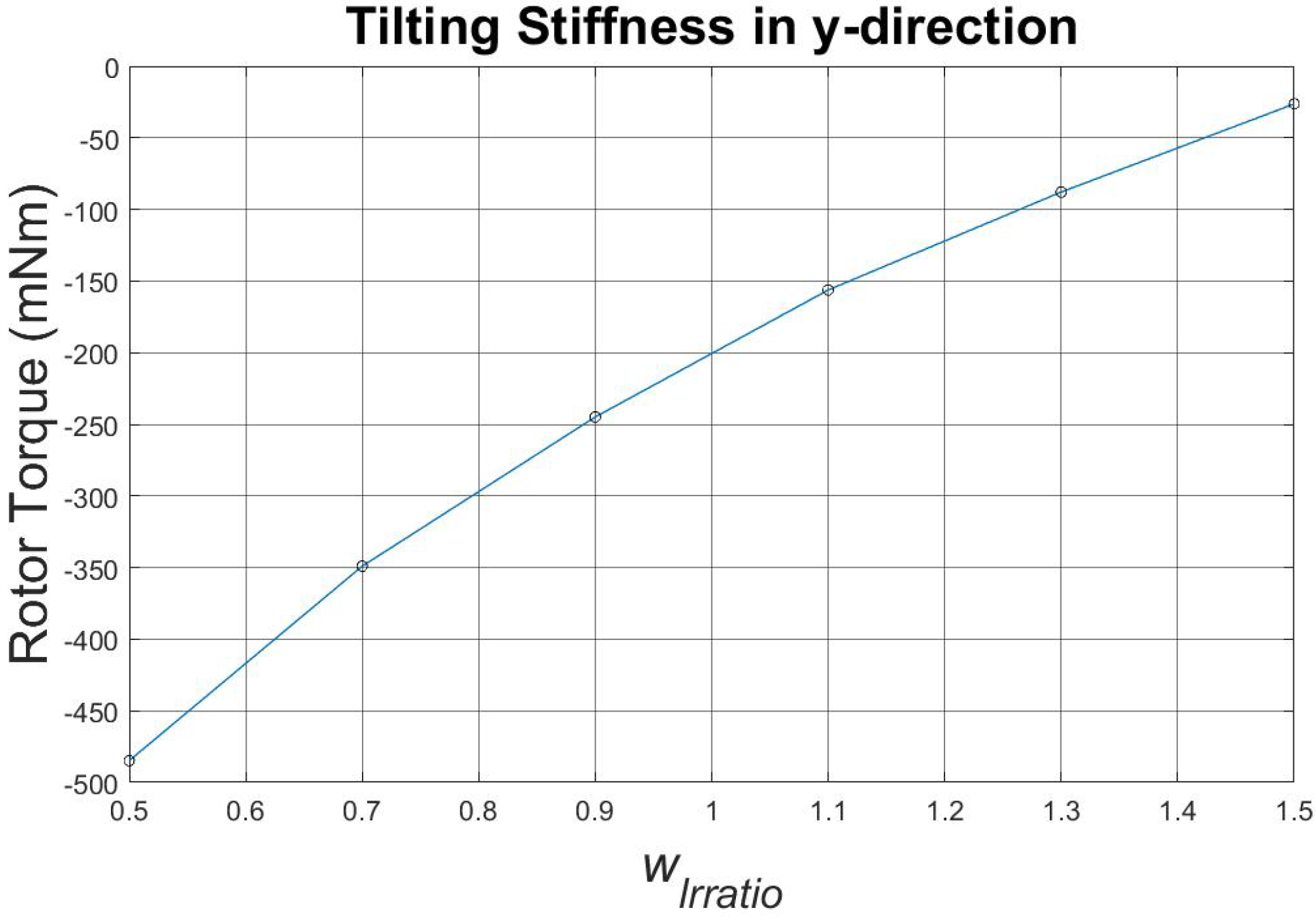
Figure 11.
Tilting stiffness in the y-direction over the parameter
As shown in Figure 10, the motor torque is higher for higher values of the parameter , while in Figure 11, the absolute tilting stiffness is higher for lower values of the parameter. Since, for both characteristics, it is better to achieve higher absolute values, a compromise of the parameter had to be made, which set the parameter as one.
In a second step, simulations with different parameters and were conducted. Since the space between the stator teeth was previously set to one by parameter , to be able to simulate and see the differences in motor performance for the other two parameters and , the motor model was redefined so that parameters and were no longer independent of each other. Thus, the parameter is defined as follows:
Based on Table 8, the parameter is defined to be 0.9. Although the motor torque and the passive stiffness do not feature their maximum, this value does not increase the cogging torque nor the cogging forces. is then set to 1.05, calculated by Equation (9).
Table 8.
Simulation results for different values of .
- Step 4:
- Rotor geometry.
After defining all the stator parameters of the FSPM properly, the drive already showed enhanced performance. Further improvement is achieved by optimizing the rotor parameters. The simulation parameters are summarized in Table 9.
Table 9.
FE simulation information of the rotor parameters.
The simulation results are shown in Table 10, Table 11 and Table 12 for the parameters and . Apart from high torque performance, cogging torque and cogging forces had an impact in defining the rotor parameters. Due to high cogging torque and cogging forces with some values of the parameters and , these parameters could not be selected with their highest passive stiffness, active torque and force values. Thus, parameter was set as 1.1 instead of 1.3, while parameter was set as 0.6 instead of 0.8. The cogging torque and cogging forces did not have an impact on choosing the parameter . Thus, this parameter was set as 0.4 with the highest results of passive stiffness, active torque and force values. The selected parameters are shown in Table 10, Table 11 and Table 12.
Table 10.
Simulation results for different values of .
Table 11.
Simulation results for different values of .
Table 12.
Simulation results for different values of .
The main goal of the optimization was to enhance the active torque and bearing forces at the cost of radial stiffness. Additionally, increasing the stabilizing tilting stiffness in the x- and y-directions is important. The final results of the optimized FSPM motor in comparison to the unoptimized version are shown in Table 13.
Table 13.
Final results and comparison of the unoptimized and optimized FSPM motor.
Results show an increase of 52.71% in axial stiffness , as well as 23.75% and 14.87% in tilting stiffness in the x-direction and in the y-direction. The radial stiffness values and were increased, which is unfavorable, but they were compensated with an increase of the active bearing forces (1000 At) and (1000 At). A beneficial increase of 132.02% in motor torque (1000 At) was achieved. Geometric parameters of the FSPM after the optimization with a comparison to the parameters before the optimization are presented in Table 14. Finally, a model of the new FSPM motor is shown in Figure 12.
Table 14.
Geometric parameters of the FSPM after the optimization.
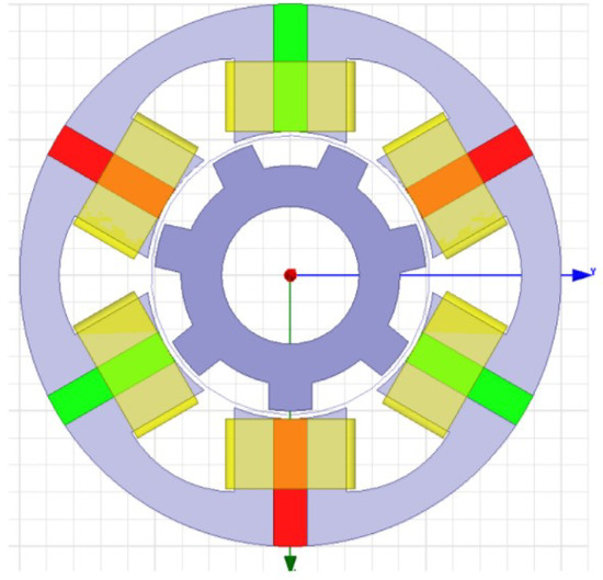
Figure 12.
New optimized FSPM motor as illustrated in the FEM program.
6. Conclusions
In this research, the main goals are topology choice and optimization of the new FSPM model. Another possible bearingless FSPM topology is introduced. In addition to an existing FSPM prototype, with this research, a setup with only six stator teeth and seven rotor poles is considered. The new motor model is able to compensate passive stabilization and generate active torque and bearing forces. Furthermore, the geometry is optimized by simulations. The novel drive features a combined winding set, where each phase generates both motor torque and bearing force. The main advantages with this motor construction are reduced financial and construction costs by the usage of the combined winding set. A disadvantage of this research is that not all performance criteria can be satisfied. More precisely, also the unfavorable radial stiffness is increased, which is compensated with increased active radial forces. Because of cogging torque and cogging forces, some parameters had to be chosen aside from their maximum. This motor topology represents an innovation in the bearingless drive industry. Based on results of this research, a new FPSM prototype is possible.
Author Contributions
V.J. applied mathematical and computational techniques, worked with the software in designing the model and wrote the initial draft under the supervision of N.B. and W.G. who, additionally, guided with ideas and reviewed and edited the original draft. W.G. acquired funding, study materials and computing resources.
Funding
This research received no external funding.
Acknowledgments
The authors thank the Institute for Electric Drives and Power Electronics, Johannes Kepler University Linz, Austria, for enabling this work. This work has been supported by the “LCM - K2 Center for Symbiotic Mechatronics” within the framework of the Austrian COMET-K2 program.
Conflicts of Interest
The authors declare no conflict of interest.
Abbreviations
The following abbreviations are used in this manuscript:
| FEM | Finite element method |
| PM | Permanent magnet |
| FSPM | Flux-switching slice motor |
| EMF | Electromotive force |
| MMF | Magneto-motive force |
References
- Bichsel, J. Beitrage Zum Lagerlosen Elektromotor. Ph.D Thesis, ETH Zurich, Zürich, Switzerland, 1990. [Google Scholar]
- Chiba, A.; Power, D.T.; Rahman, M.A. No load characteristics of a bearingless induction motor. In Proceedings of the IEEE IAS Annual Meeting, Dearborn, MI, USA, 28 September–4 October 1991; pp. 126–132. [Google Scholar]
- Salazar, A.O.; Chiba, A.; Fukao, T. A Review of Developments in Bearingless Motors. In Proceedings of the 7th International Symposium on Magnetic Bearings (ISMB7), Zürich, Switzerland, 23–25 August 2000. [Google Scholar]
- Chiba, A.; Fukao, T.; Ichikawa, O.; Oshima, M.; Takemoto, M.; Dorrell, D.G. Magnetic Bearings and Bearingless Drives; Elsevier-Newness: Oxford, UK, 2005. [Google Scholar]
- Schweitzer, G.; Maslen, E. Magnetic Bearing Theory, Design and Application to Rotating Machinery; Springer: Berlin/Heidelberg, Germany, 2009. [Google Scholar]
- Schöb, R.; Barletta, N. Principle and Application of a Bearingless Slice Motor. JSME Int. J. Ser. C Mech. Syst, Mach. Ele. Manufact. 1997, 40, 593–598. [Google Scholar]
- Gruber, W.; Silber, S.; Amrhein, W.; Nussbaumer, T. Design Variants of the Bearingless Segment Motor. In Proceedings of the International Symposium on Power Electronics, Electrical Drives, Automation and Motion, Pisa, Italy, 10–16 June 2010; pp. 1448–1453. [Google Scholar]
- Karutz, P.; Nussbaumer, T.; Kolar, J.W. Magnetically levitated slice motors—An overview. In Proceedings of the Energy Conversion Congress and Exposition, San Jose, CA, USA, 20–24 September 2009; pp. 1494–1501. [Google Scholar]
- Radman, K.; Bulić, N.; Gruber, W. Performance Evaluation of a Bearingless Flux-switching Slice Motor. In Proceedings of the Energy Conversion Congress and Exposition (ECCE), Pittsburgh, PA, USA, 14–18 September 2014. [Google Scholar]
- Okada, Y.; Yamashiro, N.; Ohmori, K.; Masuzawa, T.; Yamane, T.; Konishi, Y.; Ueno, S. Mixed Flow Artificial Heart Pump with Axial Self-Bearing Motor. IEEE/ASME Trans. Mech. 2005, 10, 1494–1501. [Google Scholar] [CrossRef]
- Raggl, K.; Kolar, J.W.; Nussbaumer, T. Comparison of Winding Concepts for Bearingless Pumps. In Proceedings of the 7th International Conference on Power Electronics, Daegu, Korea, 22–26 October 2007. [Google Scholar]
- Gruber, W.; Briewasser, W.; Rothböck, M.; Schöb, R. Bearingless slice motor concepts without permanent magnet. In Proceedings of the IEEE Industrial Conference on Industrial Technology (ICIT), Cape Town, South Africa, 25–28 February 2013. [Google Scholar]
- Gruber, W.; Bauer, W.; Radman, K. Comparison of Homopolar and Heterpolar Bearingless Reluctance Slice Motor Prototypes. Proc. Inst. Mech. Eng. Part I J. Syst. Control Eng. 2016, 231, 339–347. [Google Scholar] [CrossRef]
- Silber, S.; Amrhein, W. Bearingless Single-Phase Motor with Concentrated Full Pitch Windings in Exterior Rotor Design. In Proceedings of the 6th International Symposium on Magnetic Bearings (ISMB6), Cambridge, MA, USA, 5–7 August 1998; pp. 476–485. [Google Scholar]
- Grabner, H.; Amrhein, W.; Silber, S.; Gruber, W. Nonlinear Feedback Control of a Bearingless Brushless DC Motor. IEEE/ASME Trans. Mech. 2010, 15, 40–47. [Google Scholar] [CrossRef]
- Radman, K.; Bulić, N.; Gruber, W. Geometry Optimization of a Bearingless Flux-switching Slice Motor. In Proceedings of the Electric Machines and Drives Conference (IEMDC), Coeur d’Alene, ID, USA, 10–13 May 2015. [Google Scholar]
- Islam, M.S.; Mir, S.; Sebastian, T. Issues in reducing the Cogging Torque of Mass-Produced permament-magnet Brushless DC Motor. IEEE Trans. Ind. Appl. 2004, 40, 813–820. [Google Scholar] [CrossRef]


© 2018 by the authors. Licensee MDPI, Basel, Switzerland. This article is an open access article distributed under the terms and conditions of the Creative Commons Attribution (CC BY) license (http://creativecommons.org/licenses/by/4.0/).