Optimization of Microchannel Heat Sinks Using Prey-Predator Algorithm and Artificial Neural Networks


Abstract
1. Introduction
2. Literature Review
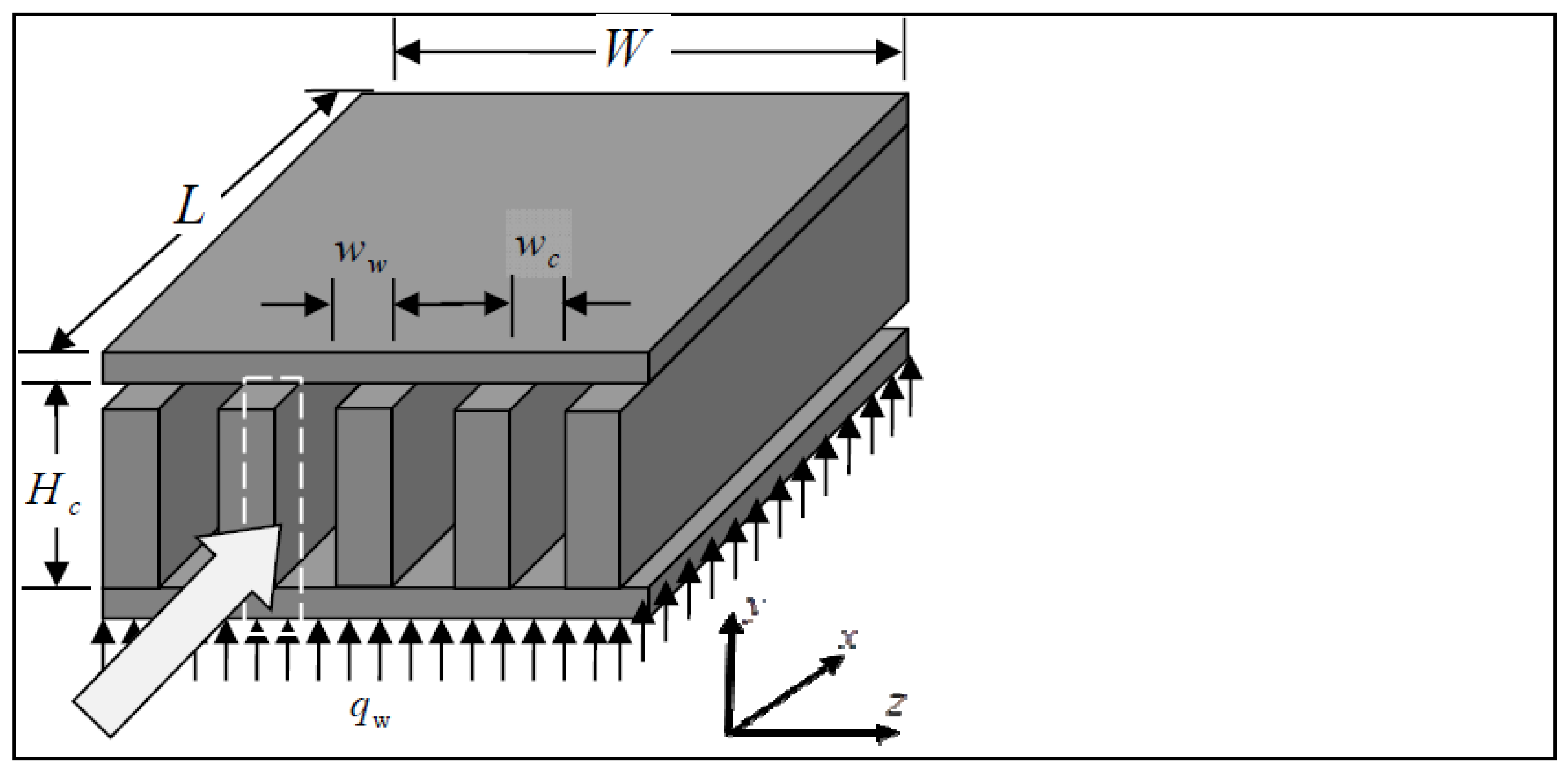
3. Microchannel Heat Sinks
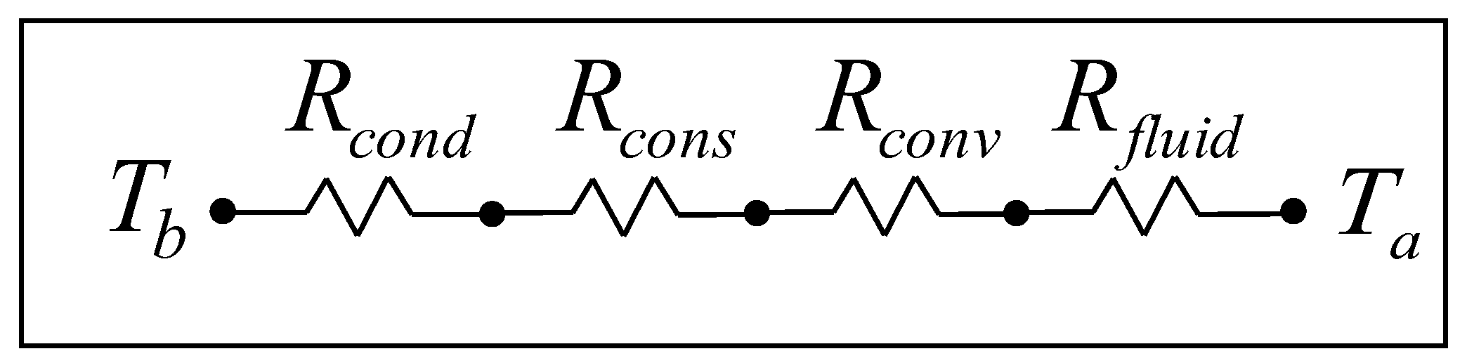
3.1. Thermal Resistance Model
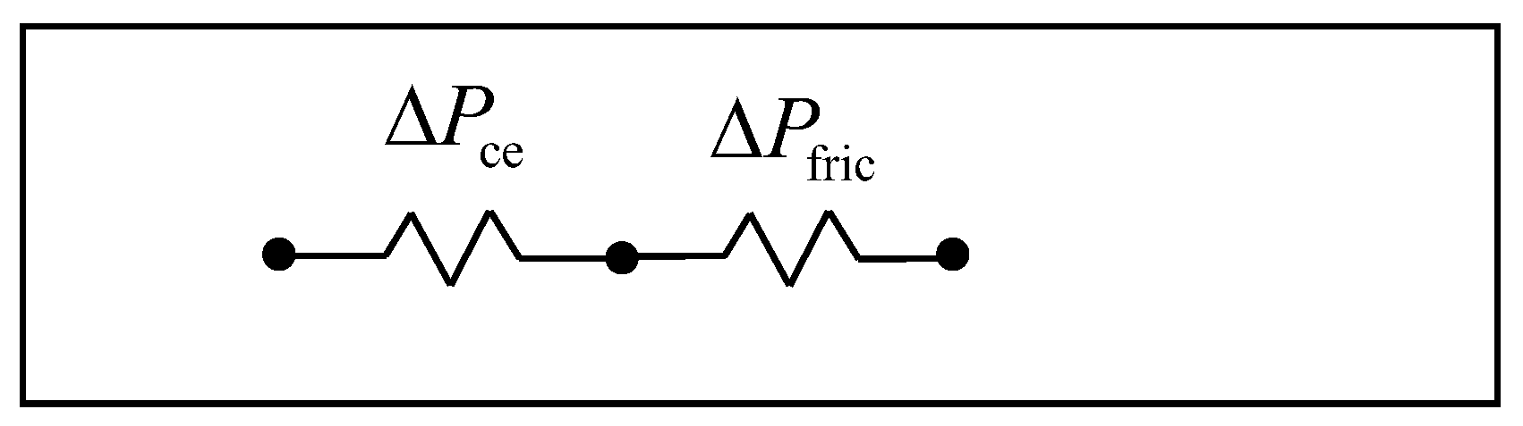
3.2. Pressure Drop Model
4. Solution Approach
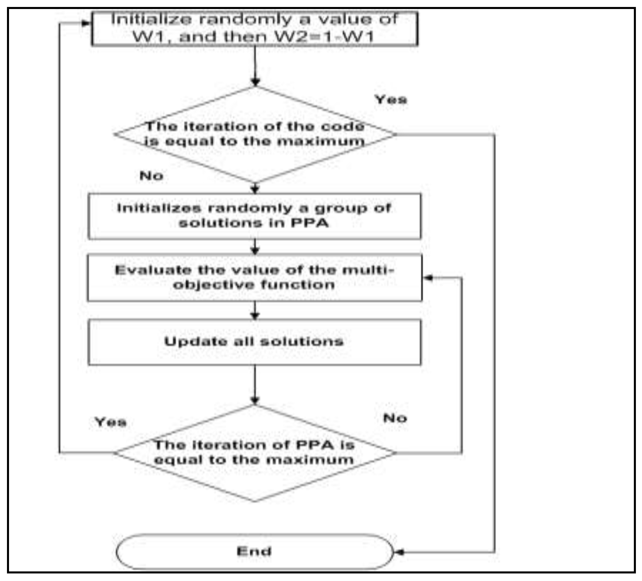
4.1. Prey–Predator Algorithm (PPA)
| Algorithm 1. Prey–predator algorithm. |
| Algorithm parameter setup |
| Generate a set of random solution, {x1, x2, …, xN} |
| For Iteration = 1:MaximumIteration |
| Calculate the intensity for each solution, {I1, I2, …, IN} and without losing |
| generality sort them in brightness from x1 dimmer to xN brightest |
| Update the predator x1 using Equation (13) |
| For I = 2:N − 1 |
| If probability_followup ≤ rand |
| For j = i + 1:N |
| Move solution i towards solution j using Equation (18) |
| End |
| Else |
| Move solution j using Equation (19) |
| End |
| End |
| Move the best solution, xN, in a promising direction using Equation (20) |
| end |
| Return the best result |
- (i)
- If follow up probability is met:
- (ii)
- If the follow-up probability is not met:Movement of the best prey:Movement of predator:
Optimization Using the Prey–Predator Algorithm
4.2. Radial Basis Function Neural Networks
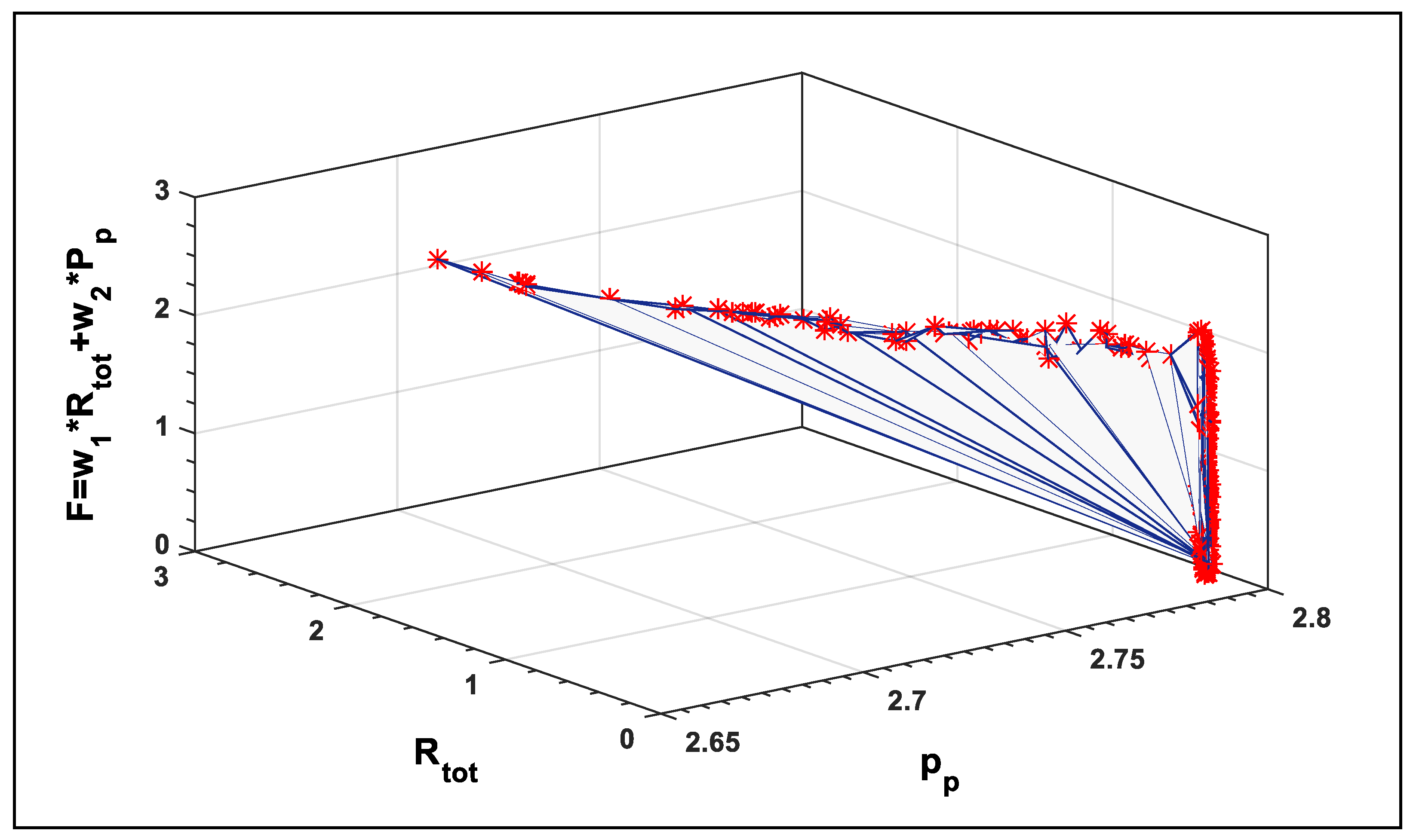
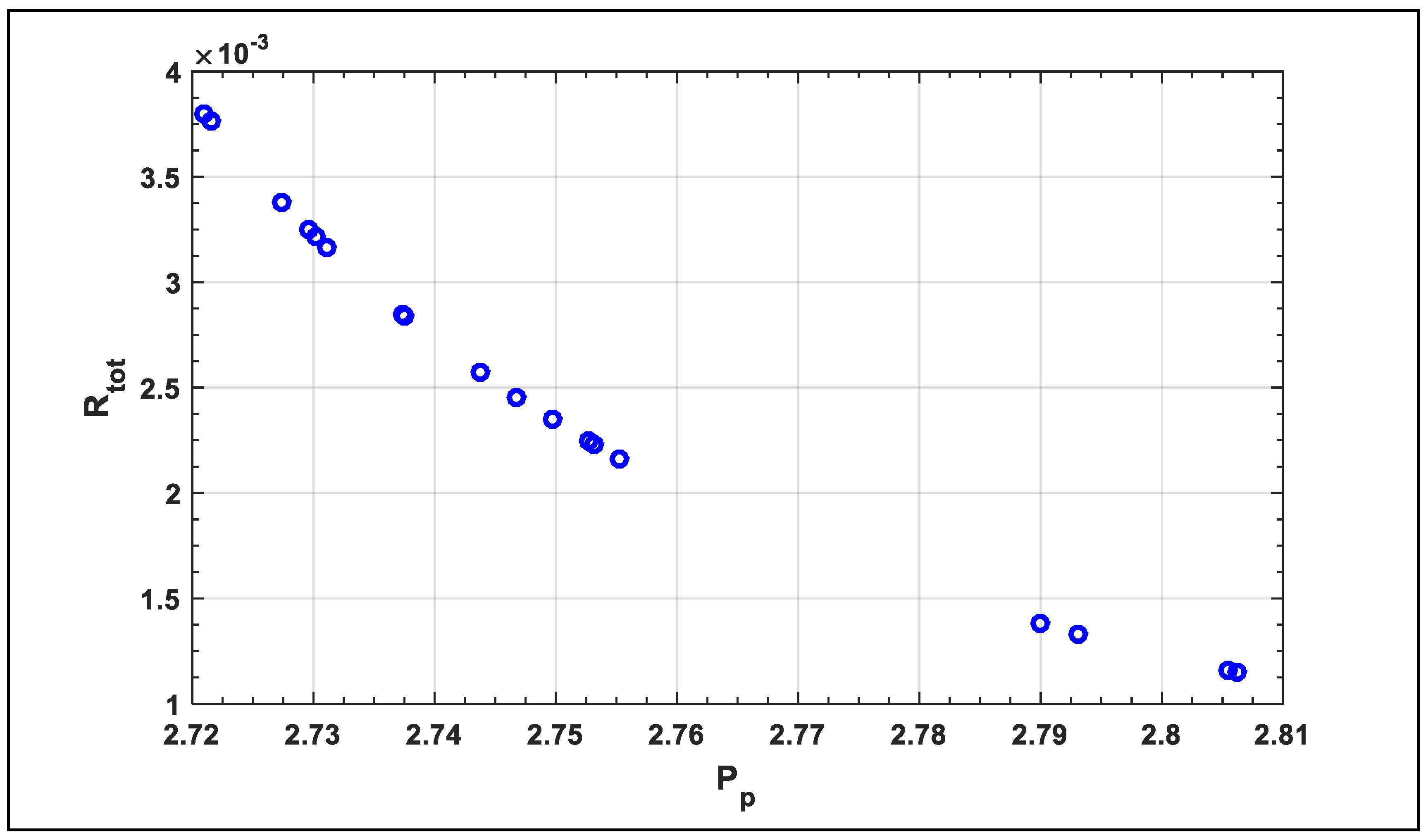
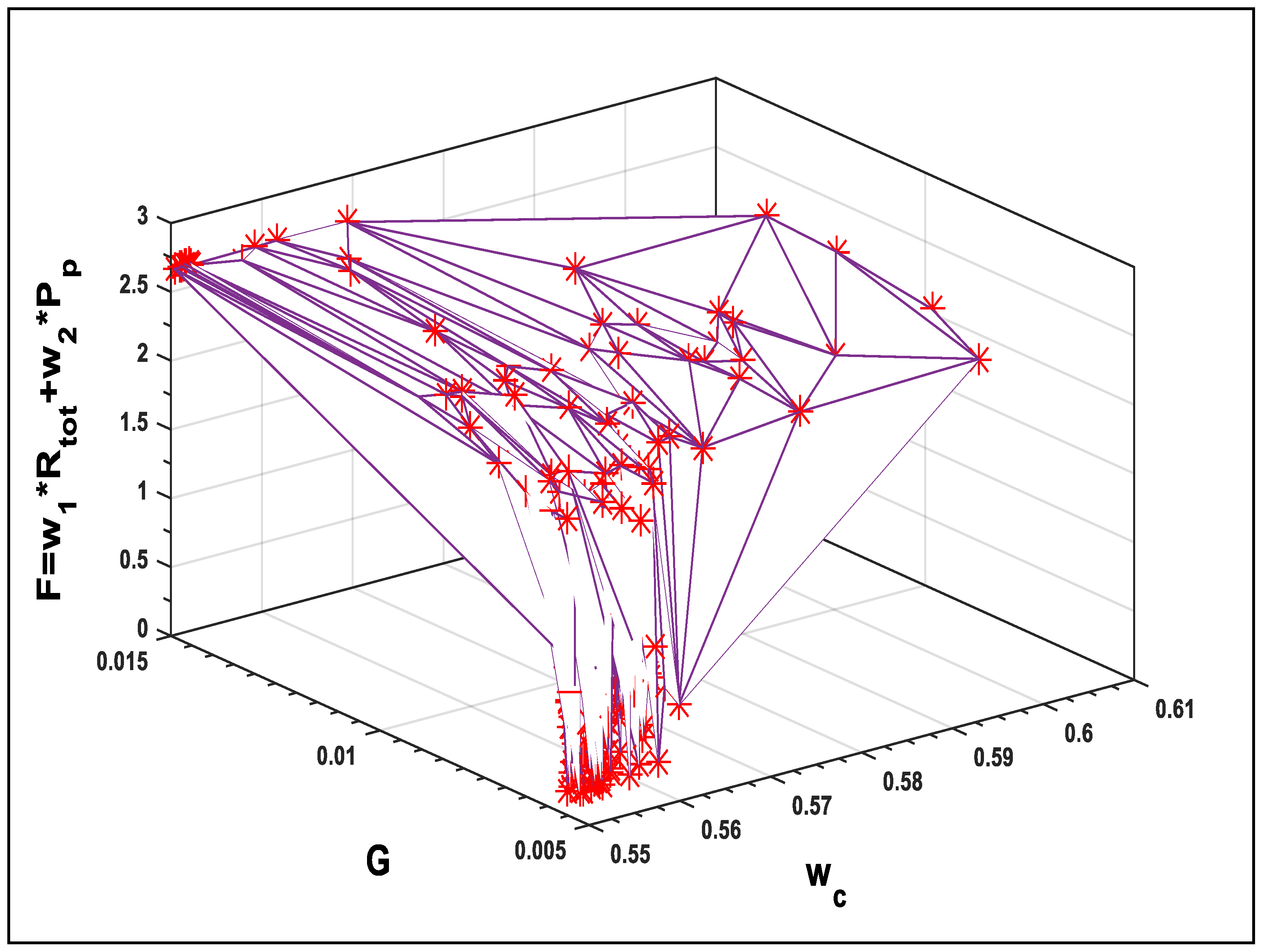
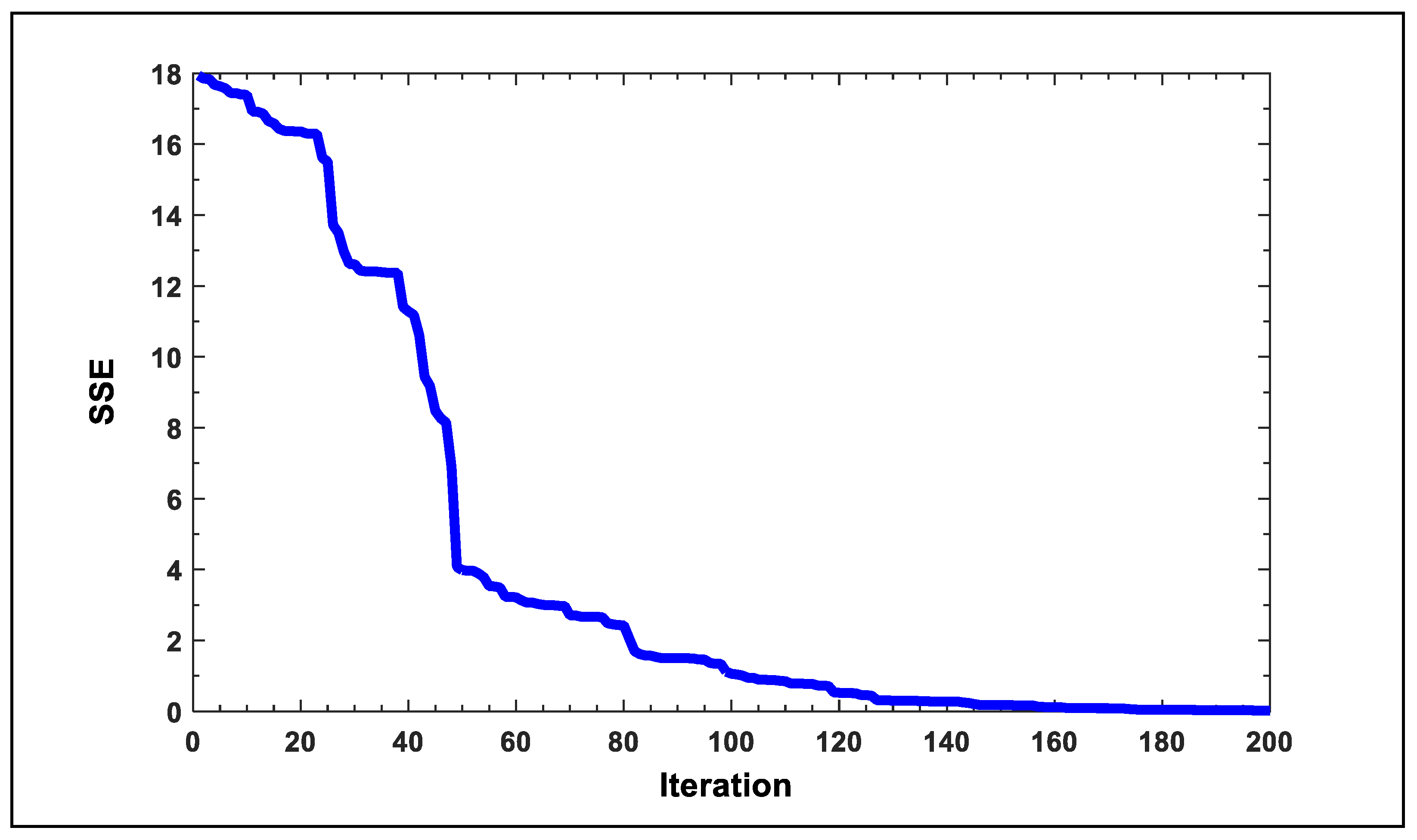
5. Results and Discussion
6. Conclusions
Author Contributions
Funding
Conflicts of Interest
Nomenclature
| A | Total surface area (m2) |
| Ac | Cross-sectional area of a single fin (m2) |
| Dh | Hydraulic diameter (m) |
| f | Friction factor |
| G | Volume flow rate (m3·s−1) |
| Hc | Channel height (m) |
| hav | Average heat transfer coefficient (W·m−2·K−1) |
| k | Thermal conductivity (W·m−1·K−1) |
| L | Length of channel in flow direction (m) |
| m | Fin parameter (m−1) |
| Mass flow rate (kg·s−1) | |
| n | Total number of channels |
| NuDh | Nusselt number based on hydraulic diameter |
| P | Pressure (Pa) |
| Pr | Prandtl number |
| R | Resistance (K·W−1) |
| ReDh | Reynolds number based on hydraulic diameter |
| Q | Heat transfer rate (W) |
| q | Uniform heat flux (W·m−2) |
| Sgen | Total entropy generation rate |
| T | Absolute temperature (K) |
| t | Thickness (m) |
| Uc | Average velocity in channels (ms−1) |
| W | Width of heat sink (m) |
| w | Width (m) |
| Greek letters | |
| α | Channel aspect ratio (≡ Hc/wc) |
| β | Fin aspect ratio (≡ ww/wc) |
| η | Fin efficiency |
| γ | Ratio of specific heats |
| ΔP | Pressure drop across microchannel (Pa) |
| ρ | Density (kg·m3) |
| ν | Kinematic viscosity (m2·s−1) |
| Subscripts | |
| a | Ambient |
| av | Average |
| b | Base plate |
| c | Channel |
| ce | Contraction/Expansion |
| cond | Conduction |
| cons | Constrictive |
| conv | Convection |
| Dh | Hydraulic diameter |
| f | Fluid |
| fric | Friction |
| p | Power |
| tot | Total |
| w | Wall or Fin |
References
- Salman, B.; Mohammed, H.; Munisamy, K.; Kherbeet, A.S. Characteristics of heat transfer and fluid flow in microtube and microchannel using conventional fluids and nanofluids: A review. Renew. Sustain. Energy Rev. 2013, 28, 848–880. [Google Scholar] [CrossRef]
- Jang, S.P.; Choi, S.U. Cooling performance of a microchannel heat sink with nanofluids. Appl. Therm. Eng. 2006, 26, 2457–2463. [Google Scholar] [CrossRef]
- Chein, R.; Chen, J. Numerical study of the inlet/outlet arrangement effect on microchannel heat sink performance. Int. J. Therm. Sci. 2009, 48, 1627–1638. [Google Scholar] [CrossRef]
- Gong, L.; Kota, K.; Tao, W.; Joshi, Y. Parametric numerical study of flow and heat transfer in microchannels with wavy walls. J. Heat Transf. 2011, 133, 051702. [Google Scholar] [CrossRef]
- Tuckerman, D.B.; Pease, R.F.W. High-performance heat sinking for VLSI. IEEE Electron Device Lett. 1981, 2, 126–129. [Google Scholar] [CrossRef]
- Zhang, C.; Lian, Y.; Yu, X.; Liu, W.; Teng, J.; Xu, T.; Hsu, C.-H.; Chang, Y.-J.; Greif, R. Numerical and experimental studies on laminar hydrodynamic and thermal characteristics in fractal-like microchannel networks. Part A: Comparisons of two numerical analysis methods on friction factor and Nusselt number. Int. J. Heat Mass Transf. 2013, 66, 930–938. [Google Scholar] [CrossRef]
- Seyf, H.R.; Feizbakhshi, M. Computational analysis of nanofluid effects on convective heat transfer enhancement of micro-pin-fin heat sinks. Int. J. Therm. Sci. 2012, 58, 168–179. [Google Scholar] [CrossRef]
- Rajabifar, B.; Seyf, H.R.; Zhang, Y.; Khanna, S.K. Flow and heat transfer in micro pin fin heat sinks with nano-encapsulated phase change materials. J. Heat Transf. 2016, 138, 062401. [Google Scholar] [CrossRef]
- Seyf, H.R.; Zhou, Z.; Ma, H.; Zhang, Y. Three dimensional numerical study of heat-transfer enhancement by nano-encapsulated phase change material slurry in microtube heat sinks with tangential impingement. Int. J. Heat Mass Transf. 2013, 56, 561–573. [Google Scholar] [CrossRef]
- Seyf, H.R.; Layeghi, M. Numerical analysis of convective heat transfer from an elliptic pin fin heat sink with and without metal foam insert. J. Heat Transf. 2010, 132, 071401. [Google Scholar] [CrossRef]
- Short, B.E.; Raad, P.E.; Price, D.C. Performance of pin fin cast aluminum coldwalls, part 1: Friction factor correlations. J. Thermophys. Heat Transf. 2002, 16, 389–396. [Google Scholar] [CrossRef]
- John, T.; Mathew, B.; Hegab, H. Parametric study on the combined thermal and hydraulic performance of single phase micro pin-fin heat sinks part I: Square and circle geometries. Int. J. Therm. Sci. 2010, 49, 2177–2190. [Google Scholar] [CrossRef]
- Tullius, J.; Tullius, T.; Bayazitoglu, Y. Optimization of short micro pin fins in minichannels. Int. J. Heat Mass Transf. 2012, 55, 3921–3932. [Google Scholar] [CrossRef]
- Adewumi, O.; Bello-Ochende, T.; Meyer, J.P. Constructal design of combined microchannel and micro pin fins for electronic cooling. Int. J. Heat Mass Transf. 2013, 66, 315–323. [Google Scholar] [CrossRef]
- Abdoli, A.; Jimenez, G.; Dulikravich, G.S. Thermo-fluid analysis of micro pin-fin array cooling configurations for high heat fluxes with a hot spot. Int. J. Therm. Sci. 2015, 90, 290–297. [Google Scholar] [CrossRef]
- Vanapalli, S.; ter Brake, H.J.; Jansen, H.V.; Burger, J.F.; Holland, H.J.; Veenstra, T.; Elwenspoek, M.C. Pressure drop of laminar gas flows in a microchannel containing various pillar matrices. J. Micromechan. Microeng. 2007, 17, 1381–1386. [Google Scholar] [CrossRef]
- Tilahun, S.L.; Ong, H.C. Prey-predator algorithm: A new metaheuristic algorithm for optimization problems. Int. J. Inf. Technol. Decis. Mak. 2015, 14, 1331–1352. [Google Scholar] [CrossRef]
- Hamadneh, N.; Khan, W.A.; Sathasivam, S.; Ong, H.C. Design optimization of pin fin geometry using particle swarm optimization algorithm. PLoS ONE 2013, 8, e66080. [Google Scholar] [CrossRef] [PubMed]
- Hamadneh, N.; Tilahun, S.L.; Sathasivam, S.; Choon, O.H. Prey-predator algorithm as a new optimization technique using in radial basis function neural networks. Res. J. Appl. Sci. 2013, 8, 383–387. [Google Scholar]
- Chou, J.-S.; Ngo, N.-T. Modified firefly algorithm for multidimensional optimization in structural design problems. Struct. Multidiscip. Optim. 2016, 1–16. [Google Scholar] [CrossRef]
- Tilahun, S.L.; Ong, H.C. Bus timetabling as a fuzzy multiobjective optimization problem using preference-based genetic algorithm. Promet Traff. Transp. 2012, 24, 183–191. [Google Scholar] [CrossRef]
- Khan, W.S.; Hamadneh, N.N.; Khan, W.A. Prediction of thermal conductivity of polyvinylpyrrolidone (PVP) electrospun nanocomposite fibers using artificial neural network and prey-predator algorithm. PLoS ONE 2017, 12, e0183920. [Google Scholar] [CrossRef] [PubMed]
- Tilahun, S.L.; Goshu, N.N.; Ngnotchouye, J.M.T. Prey Predator Algorithm for Travelling Salesman Problem: Application on the Ethiopian Tourism Sites. In Handbook of Research on Holistic Optimization Techniques in the Hospitality, Tourism, and Travel Industry; IGI Global: Hershey, PA, USA, 2016; pp. 400–422. [Google Scholar]
- Tilahun, S.L. Prey predator hyperheuristic. Appl. Soft Comput. 2017, 59, 104–114. [Google Scholar] [CrossRef]
- Tilahun, S.L.; Ong, H.C.; Ngnotchouye, J.M.T. Extended Prey-Predator Algorithm with a Group Hunting Scenario. Adv. Oper. Res. 2016, 2016, 1–14. [Google Scholar] [CrossRef]
- Tilahun, S.L.; Ngnotchouye, J.M.T.; Hamadneh, N.N. Continuous versions of firefly algorithm: A review. Artif. Intell. Rev. 2017, 1–48. [Google Scholar] [CrossRef]
- Ong, H.C.; Tilahun, S.L.; Lee, W.S.; Ngnotchouye, J.M.T. Comparative Study of Prey Predator Algorithm and Firefly Algorithm. Intell. Autom. Soft Comput. 2017, 1–8. [Google Scholar] [CrossRef]
- Lee, S.; Ha, J.; Zokhirova, M.; Moon, H.; Lee, J. Background Information of Deep Learning for Structural Engineering. Arch. Comput. Methods Eng. 2017, 25, 121–129. [Google Scholar] [CrossRef]
- Adetiba, E.; Olugbara, O.O. Improved classification of lung cancer using radial basis function neural network with affine transforms of voss representation. PLoS ONE 2015, 10, e0143542. [Google Scholar] [CrossRef] [PubMed]
- Hamadneh, N. Logic Programming in Radial Basis Function Neural Networks; Universiti Sains Malaysia: Penang, Malaysia, 2013. [Google Scholar]
- Hamadneh, N.; Sathasivam, S.; Choon, O.H. Higher order logic programming in radial basis function neural network. Appl. Math. Sci. 2012, 6, 115–127. [Google Scholar]
- Khan, W.A.; Yovanovich, M.; Culham, J.R. Optimization of microchannel heat sinks using entropy generation minimization method. IEEE Trans. Compon. Packag. Technol. 2009, 32, 243–251. [Google Scholar] [CrossRef]
- Abbassi, H. Entropy generation analysis in a uniformly heated microchannel heat sink. Energy 2007, 32, 1932–1947. [Google Scholar] [CrossRef]
- Adham, A.M.; Mohd-Ghazali, N.; Ahmad, R. Optimization of a rectangular microchannel heat sink using entropy generation minimization (EGM) and genetic algorithm (GA). Arab. J. Sci. Eng. 2014, 39, 7211–7222. [Google Scholar] [CrossRef]
- Chen, K. Second-law analysis and optimization of microchannel flows subjected to different thermal boundary conditions. Int. J. Energy Res. 2005, 29, 249–263. [Google Scholar] [CrossRef]
- Li, J.; Kleinstreuer, C. Entropy generation analysis for nanofluid flow in microchannels. J. Heat Transf. 2010, 132, 122401. [Google Scholar] [CrossRef]
- Adham, A.M.; Mohd-Ghazali, N.; Ahmad, R. Thermal and hydrodynamic analysis of microchannel heat sinks: A review. Renew. Sustain. Energy Rev. 2013, 21, 614–622. [Google Scholar] [CrossRef]
- Wang, Z.-H.; Wang, X.-D.; Yan, W.-M.; Duan, Y.-Y.; Lee, D.-J.; Xu, J.-L. Multi-parameters optimization for microchannel heat sink using inverse problem method. Int. J. Heat Mass Transf. 2011, 54, 2811–2819. [Google Scholar] [CrossRef]
- Karathanassis, I.K.; Papanicolaou, E.; Belessiotis, V.; Bergeles, G.C. Multi-objective design optimization of a micro heat sink for Concentrating Photovoltaic/Thermal (CPVT) systems using a genetic algorithm. Appl. Therm. Eng. 2013, 59, 733–744. [Google Scholar] [CrossRef]
- Ndao, S.; Peles, Y.; Jensen, M.K. Multi-objective thermal design optimization and comparative analysis of electronics cooling technologies. Int. J. Heat Mass Transf. 2009, 52, 4317–4326. [Google Scholar] [CrossRef]
- Normah, G.-M.; Oh, J.-T.; Chien, N.B.; Choi, K.-I.; Robiah, A. Comparison of the optimized thermal performance of square and circular ammonia-cooled microchannel heat sink with genetic algorithm. Energy Convers. Manag. 2015, 102, 59–65. [Google Scholar] [CrossRef]
- Khan, W.A.; Kadri, M.B.; Ali, Q. Optimization of microchannel heat sinks using genetic algorithm. Heat Transf. Eng. 2013, 34, 279–287. [Google Scholar] [CrossRef]
- Shao, B.; Sun, Z.; Wang, L. Optimization design of microchannel cooling heat sink. Int. J. Numer. Methods Heat Fluid Flow 2007, 17, 628–637. [Google Scholar] [CrossRef]
- Shao, B.; Wang, L.; Cheng, H.; Li, J. Optimization and numerical simulation of multi-layer microchannel heat sink. Procedia Eng. 2012, 31, 928–933. [Google Scholar] [CrossRef]
- Knight, R.W.; Hall, D.J.; Goodling, J.S.; Jaeger, R.C. Heat sink optimization with application to microchannels. IEEE Trans. Compon. Hybrids Manuf. Technol. 1992, 15, 832–842. [Google Scholar] [CrossRef]
- Hu, G.; Xu, S. Optimization design of microchannel heat sink based on SQP method and numerical simulation. In Proceedings of the 2009 IEEE International Conference on Applied Superconductivity and Electromagnetic Devices (ASEMD 2009), Chengdu, China, 25–27 September 2009; pp. 89–92. [Google Scholar]
- Dede, E.M. Optimization and design of a multipass branching microchannel heat sink for electronics cooling. J. Electron. Packag. 2012, 134, 041001. [Google Scholar] [CrossRef]
- Husain, A.; Kim, K.-Y. Shape optimization of micro-channel heat sink for micro-electronic cooling. IEEE Trans. Compon. Packag. Technol. 2008, 31, 322–330. [Google Scholar] [CrossRef]
- Kou, H.-S.; Lee, J.-J.; Chen, C.-W. Optimum thermal performance of microchannel heat sink by adjusting channel width and height. Int. Commun. Heat Mass Transf. 2008, 35, 577–582. [Google Scholar] [CrossRef]
- Kleiner, M.B.; Kuhn, S.; Haberger, K. High performance forced air cooling scheme employing microchannel heat exchangers. IEEE Trans. Compon. Packag. Manuf. Technol. Part A 1995, 18, 795–804. [Google Scholar] [CrossRef]
- Cruz-Duarte, J.M.; Garcia-Perez, A.; Amaya-Contreras, I.M.; Correa-Cely, C.R. Designing a microchannel heat sink with colloidal coolants through the entropy generation minimisation criterion and global optimisation algorithms. Appl. Therm. Eng. 2016, 100, 1052–1062. [Google Scholar] [CrossRef]
- Kim, S.; Kim, D. Forced convection in microstructures for electronic equipment cooling. J. Heat Transf. 1999, 121, 639–645. [Google Scholar] [CrossRef]
- Phillips, R.J. Advances in Thermal Modeling of Electronic Components and Systems; ASME: New York, NY, USA, 1990; pp. 109–184. [Google Scholar]
- Hamadneh, N.; Sathasivam, S.; Tilahun, S.L.; Choon, O.H. Learning logic programming in radial basis function network via genetic algorithm. J. Appl. Sci. 2012, 12, 840–847. [Google Scholar] [CrossRef]
- Triola, M.F. Elementary Statistics; Pearson/Addison-Wesley: Reading, MA, USA, 2006. [Google Scholar]


| Operating Conditions | Assumed Values | Operating Conditions | Assumed Values |
|---|---|---|---|
| Length of MCH, L (mm) | 51 | Specific heat of air (kJ/kg·K) | 1.007 |
| Width of MCH, W (mm) | 51 | Kinematic viscosity (m2/s) | 1.58 × 10⁻⁵ |
| Channel height, Hc (mm) | 1.7 | Prandtl number of air | 0.71 |
| Thermal conductivity of MCH (W/m·K) | 148 | Heat flux (W/cm2) | 15 |
| Thermal conductivity of air (W/m·K) | 0.0261 | Volume flow rate (m3/s) | 0.007 |
| Density of air (kg/m3) | 1.1614 | Ambient temperature (K) | 300 |
| Weight w1 | Weight w2 | wc | ww | G | N |
|---|---|---|---|---|---|
| 0.99853 | 0.001462 | 0.68274 | 0.551488 | 0.00556 | 40.87455 |
| Weights | Centers | Widths | |||
|---|---|---|---|---|---|
| ω1 | 1.08 | μ1 | 3.83 | σ1 | 1.48 |
| ω2 | 3.99 | μ2 | 1.28 | σ2 | 3 |
| ω3 | 3.99 | μ3 | 1.36 | σ3 | 1 |
| ω4 | 1.11 | μ4 | 2.76 | σ4 | 1.01 |
| ω5 | 3.78 | μ5 | 4.5 | σ5 | 2.65 |
| Source of Variation | SS | df | MS | F | p-Value | Critical Values |
|---|---|---|---|---|---|---|
| Between Groups | 0.680727 | 1 | 0.680727 | 10.44468 | 0.001299 | 0.001 |
| Within Groups | 38.32258 | 588 | 0.065174 | - | - | - |
| Total | 39.00331 | 589 | - | - | - | - |
© 2018 by the authors. Licensee MDPI, Basel, Switzerland. This article is an open access article distributed under the terms and conditions of the Creative Commons Attribution (CC BY) license (http://creativecommons.org/licenses/by/4.0/).
Share and Cite
Hamadneh, N.; Khan, W.; Tilahun, S. Optimization of Microchannel Heat Sinks Using Prey-Predator Algorithm and Artificial Neural Networks. Machines 2018, 6, 26. https://doi.org/10.3390/machines6020026
Hamadneh N, Khan W, Tilahun S. Optimization of Microchannel Heat Sinks Using Prey-Predator Algorithm and Artificial Neural Networks. Machines. 2018; 6(2):26. https://doi.org/10.3390/machines6020026
Chicago/Turabian StyleHamadneh, Nawaf, Waqar Khan, and Surafel Tilahun. 2018. "Optimization of Microchannel Heat Sinks Using Prey-Predator Algorithm and Artificial Neural Networks" Machines 6, no. 2: 26. https://doi.org/10.3390/machines6020026
APA StyleHamadneh, N., Khan, W., & Tilahun, S. (2018). Optimization of Microchannel Heat Sinks Using Prey-Predator Algorithm and Artificial Neural Networks. Machines, 6(2), 26. https://doi.org/10.3390/machines6020026