Abstract
Several multiple model adaptive control architectures have been proposed in the literature. Despite many advances in theory, the crucial question of how to synthesize the pairs model/controller in a structurally optimal way is to a large extent not addressed. In particular, it is not clear how to place the pairs model/controller is such a way that the properties of the switching algorithm (e.g., number of switches, learning transient, final performance) are optimal with respect to some criteria. In this work, we focus on the so-called multi-model unfalsified adaptive supervisory switching control (MUASSC) scheme; we define a suitable structural optimality criterion and develop algorithms for synthesizing the pairs model/controller in such a way that they are optimal with respect to the structural optimality criterion we defined. The peculiarity of the proposed optimality criterion and algorithms is that the optimization is carried out so as to optimize the entire behavior of the adaptive algorithm, i.e., both the learning transient and the steady-state response. A comparison is made with respect to the model distribution of the robust multiple model adaptive control (RMMAC), where the optimization considers only the steady-state ideal response and neglects any learning transient.
1. Introduction
Multi-model adaptive control is an emerging field that has proven to be successful in mitigating the limitations of classical adaptive control by providing faster adaptation, see [1] for examples. In this method, instead of one single parameter-varying controller, multiple fixed-parameter controllers pertaining to different operating regimes are utilized. A variant of this technique known as multi-model unfalsified adaptive supervisory switching control (MUASSC) has recently been proposed [2,3,4,5,6]. This methodology, although promising, needs further systematic analysis regarding the determination of the minimum number of pairs model/controller required and their corresponding locations (in the uncertain parameter space) to address stability and performance issues. Notice that the problem of the determination of the location and minimum number of pairs model/controller is not addressed in most adaptive control methods, with the exception of robust multiple model adaptive control (RMMAC) [7], where the determination is based on steady-state considerations, neglecting the learning transient of the adaptive method. In other words, one of the open problems in multi-model adaptive control can be stated as follows: it is not clear how to place the pairs model/controller is such a way that the properties of the switching algorithm (e.g., number of switches, learning transient, final performance) are optimal with respect to some criteria. With this work, we want to provide a better insight into how the determination of the location and minimum number of pairs model/controller can have an important effect on the transient performance of the adaptive control method. In fact, for multi-model adaptive control, switching performance (i.e., transient performance) for a given uncertainty space greatly depends on the location and number of controllers that try to tackle it. “Switching performance” refers to a number of factors, such as the extent of transients, how quickly the best controller is switched on, the highest number of switches before the best controller is in the loop, a comparison of the mixed or generalized sensitivities of the final controller/plant pair in the closed loop, etc.
The work presented addresses the aforementioned open problem by developing suitable criteria and optimization algorithms for providing structurally optimal multi-model adaptive control schemes. In particular, we will define a structural index for MUASSC and develop optimization procedures to optimize the model locations inside the uncertainty set in such a way so as to minimize the structural index. Difficulties associated with these procedures are that the cost function to be minimized is not only nonlinear, but also discontinuous. Hence, a multi-start approach along with intelligent methods to discard unnecessary starting points is used to fulfill the objective. The objective of the optimization problem can be stated as follows: given an uncertainty set, we want to find the minimum number of controllers N and their optimal locations within the set, such that certain stability and performance properties are guaranteed (structural optimality). The interest obviously lies in achieving the best possible performance with the least number of controllers due to the fact that this directly translates into lower memory and computational requirements. The peculiarity of the proposed optimality criterion and algorithms is that the optimization is carried out so as to optimize the entire behavior of the adaptive algorithm, i.e., both the learning transient and the steady-state response. To the best of the authors’ knowledge, this is the first time that the complete behavior of the switching algorithm (e.g., number of switches, learning transient, final performance) is taken into account for synthesizing the pairs model/controller. A comparison is made with respect to the model distribution of the robust multiple model adaptive control (RMMAC), where the optimization considers only the steady-state ideal response and neglects any learning transient.
The rest of the work is organized as follows. Section 2 provides more insight into the basics and fundamentals of adaptive control with switching with a focus on the developed MUASSC approach. Section 3 gives a brief background into the RMMAC scheme. Section 4 introduces a simple numerical example used for benchmarking. Section 5 develops algorithms for optimization of the MUASSC structural index. In Section 6, we propose an improvement on the optimization of the RMMAC structural index. Finally, comparative results with different multiple-model distributions are presented in Section 7.
2. Basics of Multi-Model Adaptive Control
Before the work is presented, it is essential to explore some fundamentals of multi-model-based adaptive switching control in order to understand the goals and the methodology devised to arrive at it. The present section is therefore dedicated to equip the reader with the basics of the subject.
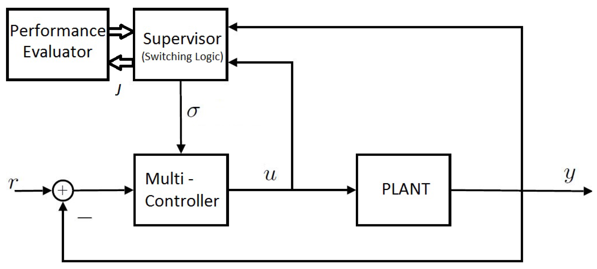
The general architecture of a multi-model adaptive control scheme consists of the four blocks shown in Figure 1: plant, multi-controller, supervisor and performance evaluator. In the following, we give an outline for each component.
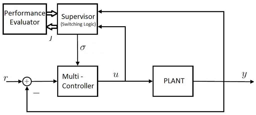
Figure 1.
General outline of the multi-model adaptive control scheme [2].
2.1. The Plant
The plant to be controlled contains uncertain parameters belonging to a known uncertainty set. The plant receives the control input u from the controller and filters it to produce the output y. Both of these signals are utilized by the supervisor in order to select the appropriate controller based on the operating region. The uncertain parameter set is divided into N different subsets, and in each subset, a representative nominal model is chosen among the following ones. It is assumed that uncertainty can take up any one of these values in a discrete manner. The density of the division must be sufficiently high, such that one has a “tight” approximation of the plant. Therefore, the discretized set attempts to approximate different models according to which the plant operates.
Here, represents the i-th model, while N represents the total number of models adopted to describe the plant. The problem is choosing these models in an optimal way with respect to stability and performance of the adaptive algorithm.
2.2. The Multi-Controller
Associated with each nominal model, there is a candidate controller, which are therefore placed in different regions of operation of the uncertainty set. Based on the current true plant parameter value, the best controller among them is switched on in the loop. The decision of the best controller to be turned on at a given instant is taken up by the supervisor, which in-turn constantly monitors a set of performance signals linked to each controller to make the above decision. The controllers that form the multi-controller are among the following ones:
Here, represents the i-th controller, and the number of controllers is the same as the number of models. Notice that not only the model location, but also the controller will contribute to the stability and performance of the adaptive scheme, as will be explained later. Furthermore, if N tends to infinity, then the performance can be guaranteed irrespective of the parameter value [8].
2.3. Performance Index Evaluator
The role of the performance evaluator is to generate a quantitative index used by the supervisor to produce the controller index σ. Based on the plant input and output data, a specialized performance index function is formulated tailored according to the family of multi-model adaptive control being used. In this work, the performance index corresponding to MUASSC will be demonstrated in detail. The performance variable value is constantly calculated at every instant of time for all of the controllers simultaneously, and based on this monitored data, the supervisor switches on the most apposite controller at that time instant. We come up with a family of performance indexes as follows:
Here, represents the performance index corresponding to the i-th pair model/controller. Different performance indices corresponding to the different families have been proposed in the literature [9,10,11,12,13].
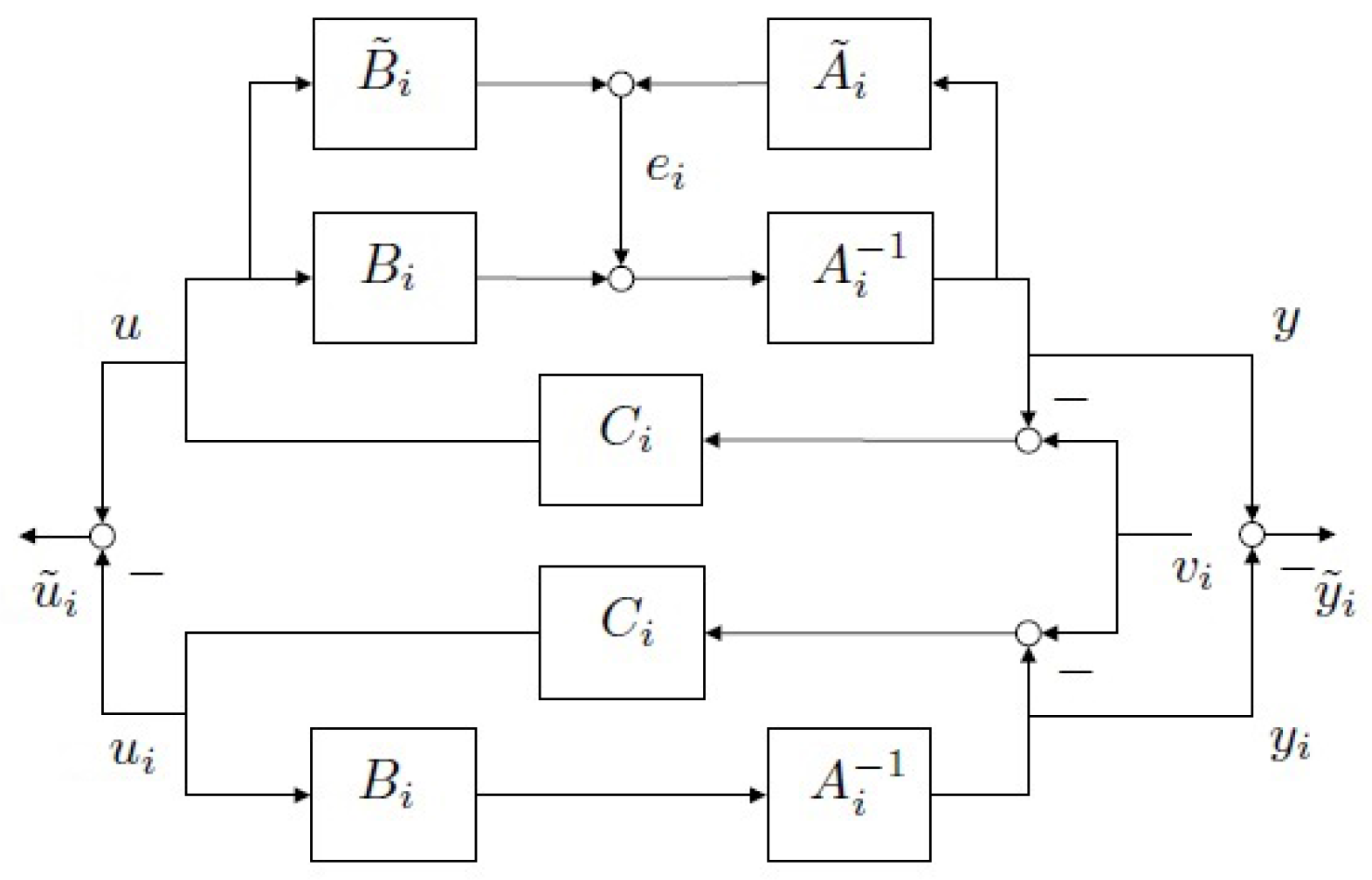
In the MUASSC scheme, the test functional is designed as follows. With reference to Figure 2, let us define:
and:
where and (where is the transfer function of the real plant). The problem of inferring the stability of the candidate loop can be approached via the estimation of the magnitude from the recorded data z. If denotes the deviation between plant and model input when driven by the current virtual reference , then the transfer function relating this deviation to the actual plant variable z coincides with the weighted generalized sensitivity matrix ():
where and , . A convenient test functional for this type of scheme involves an estimate of this generalized sensitivity matrix: ; and is approximately calculated as:
where denotes the norm of the sequence . Notice that whenever the plant uncertain set is compact and a priori known, the model distribution can be designed dense enough to ensure that, for any possible plant in the uncertainty set, there exist indices , yielding stable loops , such that , . The stabilizing indexes are denoted with . A model distribution for which such a property holds will be referred to as a β-dense model distribution. β is the maximum over all of the minima over all i of the least upper-bounds satisfying the mentioned inequality. Specifically,
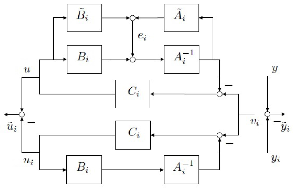
Figure 2.
Multi-model unfalsified adaptive supervisory switching control scheme (MUASSC) [2].
Further, assuming a β-dense model distribution, is said to have the β-property if .
2.4. Supervisor (Switching Logic)
The choice of controller is based on an embedded “switching” logic that assigns the controller index σ. A conventional and an intuitive switching logic would involve selecting the controller associated with the least J. This is not always sufficient, as in cases where rapid and random parameter fluctuations occur, the switching logic would constantly begin to switch between the various controllers, which in turn leads to chattering. Excessive chattering is a potential source of system instability, and therefore, to prevent such occurrences, the switching logic employs additional safety features, like hysteresis switching. While different logics other than hysteresis switching have been proposed, in the following, we will concentrate solely on the hysteresis switching logic. The following hysteresis switching logic is used [14]:
where stands for the least integer , such that , and h, a (typically small) positive real constant, known as the hysteresis constant.
As mentioned, h, which is usually a small value, is positive real. The significance of the hysteresis is that the controller index changes to the one corresponding to the better controller if and only if the improvement gain is at least as high as the hysteresis value h [14]. If the improvement in J is smaller than this, then switching to the better controller is avoided, as the action is just not worth it.
2.5. MUASSC Stability and Performance Result
If the test functional Equation (4) is adopted, in conjunction with the hysteresis switching logic Equations (6) and (7), then the following theorem is valid, as stated in the work [2].
Theorem 1.
Let z be the vector-valued sequence of I/O plant data and σ the switching sequence resulting with the choice of such a test functional as above. Then, provided that the problem feasibility holds, for any initial condition and reference r, the HSSL (Hysteresis Switching Logic) lemma holds, the resulting multi-model-based UASSC system is r-stable, and if P is compact, under a nominal model distribution , , then:
- 1.
- The total number of switches is bounded as follows:
- 2.
- The occurrence of the condition, ,ensures that no destabilizing controller will be switched-on at and after time t;
- 3.
- The occurrence of the condition, ,ensures that , , and the offset-free property to ;
- 4.
- If , each candidate controller can be switched-on no more than once, and any stabilizing controller with the β-property, once switched-on in feedback with the plant, will never be switched-off thereafter.
Meaning of Theorem 1: The theorem above suggests the benefit of decreasing β on the transient performance of the scheme. The lower the β, the lower is the upper bound on the number of switches. It is to be noted that additionally, N plays a crucial role not only in determining , but also in the value of β obtained in the first place. For a fixed uncertainty, increasing N generally leads to a lower β value and vice versa. The second and third bullets of the theorem suggest that with a lower β, the chances of an unwanted destabilizing controller being switched on in the future is further mitigated. Consequently, with a lower β and a fixed h, the chances of the condition stated in the fourth bullet of the theorem is once again more easily satisfied. Summarizing, the reduction of β will lead to the improvement of the transient “performance” of the MUASSC algorithm.
3. The Robust Multi-Model Adaptive Control Architecture
Among the different approaches proposed in multiple model adaptive control, the RMMAC is the only one where the model distribution was explicitly addressed. It is thus interesting to briefly explain the way RMMAC selects the pair model/controllers and to compare it to our proposed solution. In the following, we present only the essential points of RMMAC: for a complete overview, the reader is referred to [7]. This is a state of the art multiple model architecture, which has been proposed as another alternate approach towards addressing the problem posed by system uncertainties. An essential distinction used in this method is that the control signal generated to steer the plant is a “mixture” of control signals produced by each of the controllers of the bank, which is as depicted in the papers [7,13]. The bank of N Kalman observers plays a role in generating the probability signals with the help of the posterior probability evaluator (PPE), which are in turn multiplied with the corresponding input signals. The probability of the most suitable controller (based on region of operation) is close to one and the rest near zero. The bank of controllers contains a group of LNARCs (local non-adaptive robust controllers), which pertain to various regions of the uncertainty set. The LNARCs are designed to guarantee “local” stability and performance robustness. These are an extension of the GNARC (global non-adaptive robust controller), where one single controller is designed to handle the entire uncertainty set. Both of these types of controllers have been introduced in the sections.
3.1. Global Non-Adaptive Robust Controller
The GNARC design consists of a single non-adaptive robust controller covering the entire uncertainty set. Notice that this design is possible only if the uncertainty set is small enough. In such cases, the entire uncertainty set is approximated by a delta block, which is norm bounded by one and accompanied by a suitable scaling weight. Based on the set of models, a design methodology involving iterations is used and is termed as the “mixed μ synthesis”. The outcome of the process is a non-adaptive LTI (Linear Time Invariant) MIMO/SISO (MIMO—Multiple Input Multiple Output, SISO—Single Input Single Output) dynamic compensator with fixed parameters, which necessarily guarantees system stability and provides performance robustness (provided such a controller exists).
As explained by Athans [7]: “The ‘mixed-μ synthesis’, loosely speaking, de-tunes an optimal nominal design, that meets more stringent performance specifications, to reflect the presence of inevitable dynamic and parameter errors. In particular, if the bounds on key parameter errors are large, then the ‘mixed- μ synthesis’ yields a robust LTI design albeit with inferior performance guarantees as compared to the nominal design. So the price for stability robustness is poorer performance”. The mixed sensitivity nominal design nominal design that has been spoken of till now has been introduced by Kwakernaak in [15] and involves the minimization of the closed loop “weighted sensitivity” and the “weighted input complementary sensitivity” as a mixed minimization problem to make the system as insensitive as possible to high frequency disturbances and measurement noise and to reduce system offset (reference-output) with the minimal control effort possible. This process is accomplished by searching among a set of controllers to determine the best possible one that would minimize the mixed of the closed loop system. The ‘mixed minimization’ is done by the stacking approach as follows:
where S is the sensitivity function and the complementary sensitivity function, and and form the weights that are suitably specified by the designer. The corresponding controller is searched among all of the possible set of controllers C to yield the best controller that would satisfy the posed weights on the transfer functions and S. This is possible provided such a controller does exists in the set that is being searched. This can be expressed as follows:
Hence, an optimization routine searches among all possible C to yield the result. Once this controller is obtained, the iterations [15] can be performed to accompany for greater uncertainty robustness to creates an upper bound of . If this is <1, it means that the resulting closed loop system with this particular controller will provide guaranteed stability and maintain performance over the larger and extended uncertainty set as compared to the normal “mixed weighted sensitivity” . If not, this means no such controller exists, which can render the system closed loop stable with the currently posed performance requirements.
Before one investigates the possibility of an adaptive controller, one must be aware of the best non-adaptive GNARC controller possible. If the performance improvements are not that significant, then the GNARC method can be used to design one single controller, hereby eliminating the need for complex adaptive control.
3.2. Local Non-Adaptive Robust Controller
If the uncertainty set is too big for a single controller, then one needs to distribute numerous nominal models all over the uncertainty set. These models must be capable of tackling the required uncertainty and provide performance and stability “locally” around the localized nominal model. Hence, one utilizes the GNARC scheme of μ synthesis and iterations using the localized nominal model to generate the corresponding localized robust controller.
A special case of LNARC is the case where infinite such “local” models cover the entire uncertainty set and is termed as the FNARC (fixed non-adaptive robust controller) situation.
The non-adaptive GNARC provides the lower-bound upon expected performance, while the FNARC provides the performance upper bound. Given an accepted degradation of performance X%, the RMMAC scheme places the local controllers is such a way that the performance of the LNARC is not worse than X% the performance of FNARC. This gives an optimization criterion to optimize the model distribution. It has to be noted, however, that the performance of the RMMAC criterion is defined only in the ideal steady-state case, i.e., supposing that the switching has selected the ideal controller. No transient performance, the number of switches nor the value of the test functional (e.g., as specified in Theorem 1) is involved in the RMMAC model distribution optimization.
4. Example Plant for Comparison
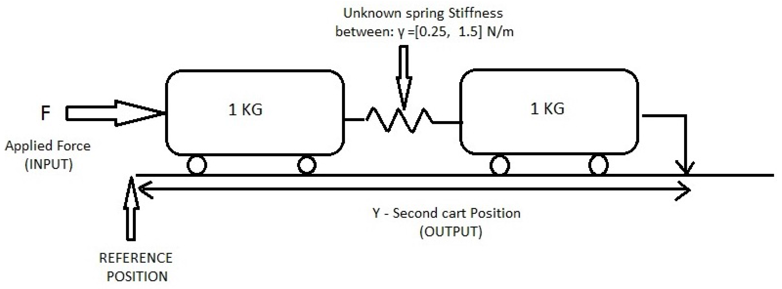
The system under analysis involves two masses of 1 kg each connected via a spring whose stiffness constant γ is the unknown parameter and can take up any value between a predetermined fixed uncertainty interval of [2]. A force is applied to the first cart (Figure 3), and the variable to be controlled is the position y of the second cart with respect to a certain reference. In order for greater clarification, a multi-controller is placed in feedback with this plant, which was devised based on the weighted mixed sensitivity criterion as described by Kwakernaak [15] as with a strictly Hurwitz polynomial. The uncertainty set of will now be the example uncertainty set for the rest of the paper, and it shall be utilized for calculating the (MUASSC and RMMAC) structural indexes by synthesizing controllers for different values of spring constants withing this given set.
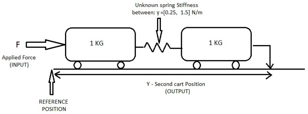
Figure 3.
Example setup.
Such mass spring systems are very popular in adaptive supervisory switching control and form a sort of benchmark. Although the mass spring system might seem academic, such models are widely used in industry to mimic the behavior of suspension systems and smart structures. The reader is referred to papers [16,17,18], which deal with the modeling of vehicle suspension systems using similar mass spring damper configurations. It would be also interesting to refer to [19], wherein flexible structures are modeled using such mass spring configurations. Such flexible structures are used in space structure applications, such as solar panel deployment mechanisms, etc.
5. Algorithms for the Attainment of MUASSC-Based Optimal Structural Index
In contrast with the RMMAC approach, in MUASSC, we make the assumption that an optimal model distribution is related to having a minimum β. This is justified by the stability and performance results stated in Theorem 1. Hereafter, β will be refereed to as the MUASSC structural index.
As , the presence of max and min operators leads to discontinuity in function values. Due to the existence of such discontinuities, optimizing the cost function directly is a difficult task. The technique devised through this work follows a multi-start approach coupled with novel tricks that take advantage of a certain structure that exists in the problem. This has been presented in the next section comprehensively.
The section is divided into five parts, which are organized to present the developed approach in a step-wise systematic manner. As a multi-start technique is devised, the first section deals with the generation of such start points following the section where clever techniques have been devised to reject a sizable portion of the generated start points. To make the techniques intuitively clear, a graphical interpretation of such rejections will be depicted. Having introduced the MUASSC structural index, we will present the algorithms aiming at minimizing it.
5.1. Minimization of MUASSC Structural Index
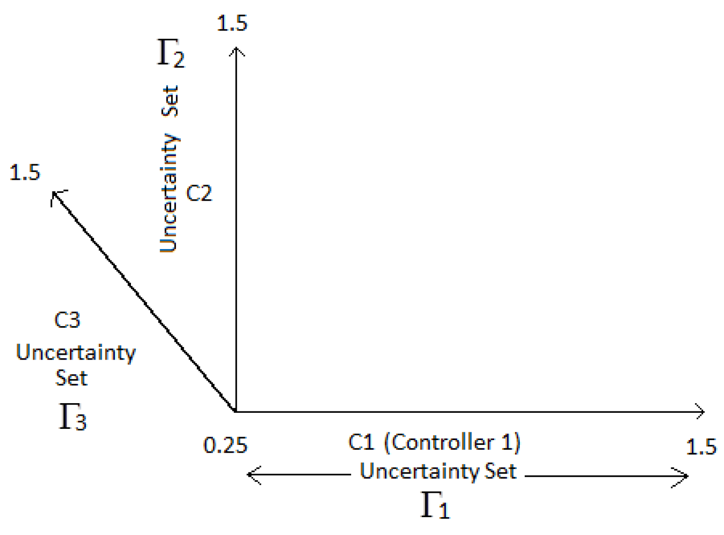
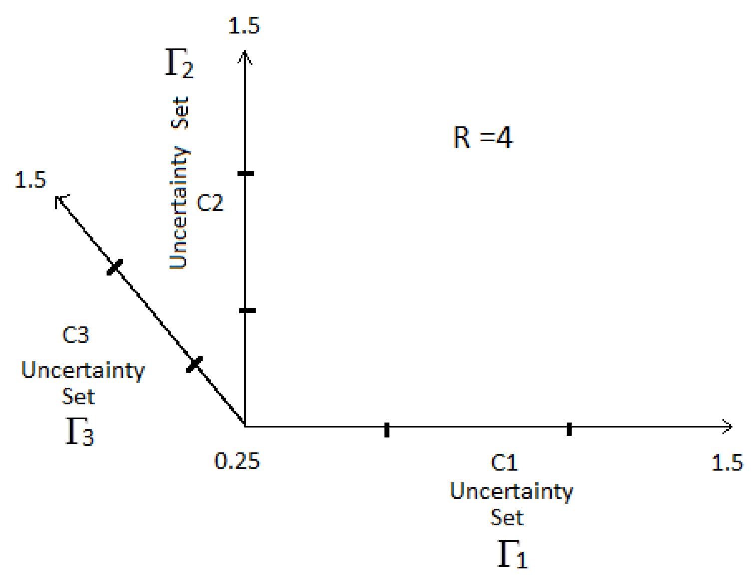
The first step towards the generation of start points lies in aligning the given uncertainty set along the three axes due to the fact that currently, three controllers have been chosen to cover the uncertainty (). Furthermore, if four or more controllers are present, the process of start point generation could not be demonstrated graphically, and hence, has been chosen for this demonstration in the first place. The aligned uncertainty of along the three axes is shown in Figure 4. Again, three such sets have been aligned, as three controllers are used. If four controllers are used, four such sets needs to be aligned with one in the fourth dimension, which cannot be visually imagined. Hence, the demonstration has been restricted to the three-dimensional case, but can very well be extended to higher dimensions if more controllers are to be used. The idea is that each controller, , and , is placed at different parts of their individual uncertainty sets, , and (which is actually the same uncertainty as ), with the corresponding β being plotted in the fourth dimension for different combinations of controller placement. This is made clear subsequently.
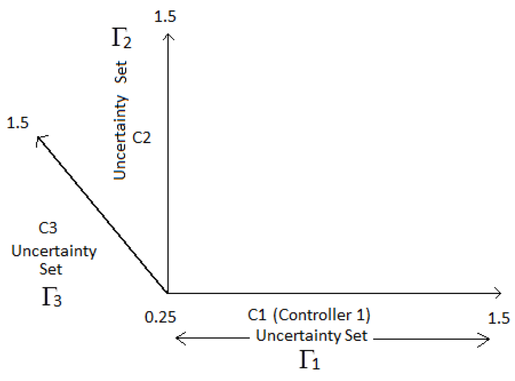
Figure 4.
Generation of start points: aligning the uncertainties based on N.
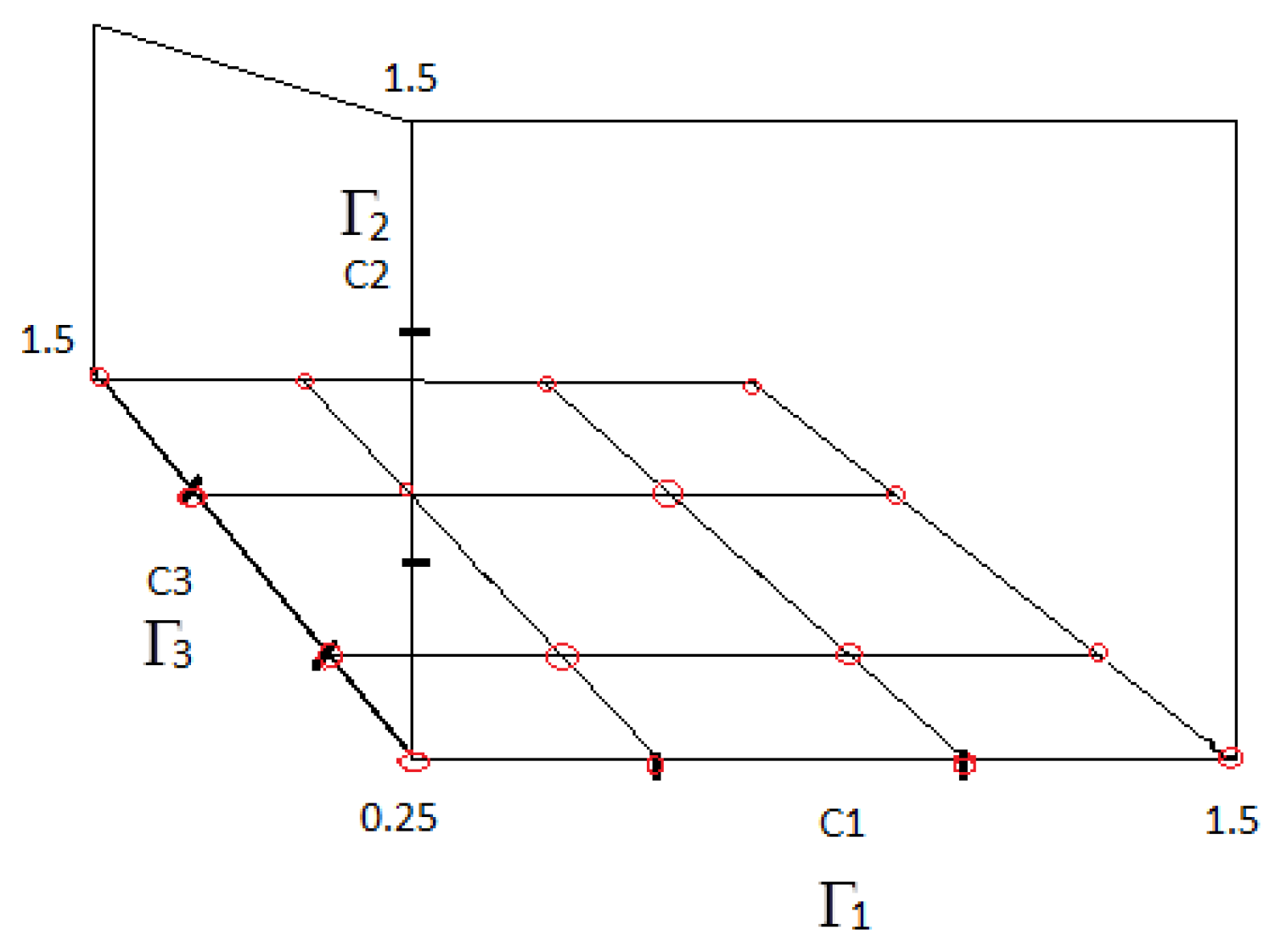
Once the uncertainty alignment is ready, one needs to determine the “Grid Resolution” R, which divides each of the three uncertainty sets, , and , into R equispaced points. As described above, the β will now be plotted in the fourth dimension, assuming that the three controllers are now synthesized for different combinations of these discrete set values (Rdivisions). For the purpose of this demonstration, a grid resolution of has been demonstrated in Figure 5. Once this is decided, the points created at the intersection of the resultant ‘grid’ formed at the base of the cuboid are taken as the first bunch of start points for the multi-start procedure. One can notice for this bunch of points that the value of the Y coordinate or is fixed. These start points have been encircled in red in Figure 6.
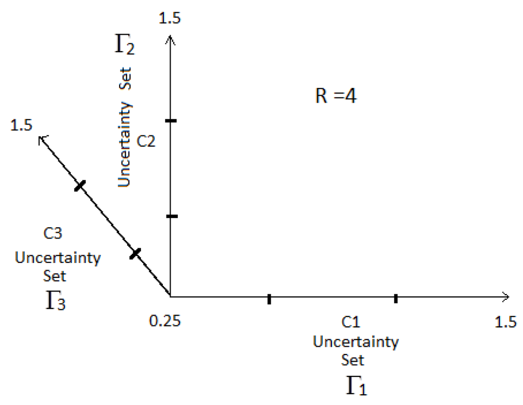
Figure 5.
Generation of start points: generation of grid .

Figure 6.
Generation of start points: generated start points from the bottom most plane of the cuboid.
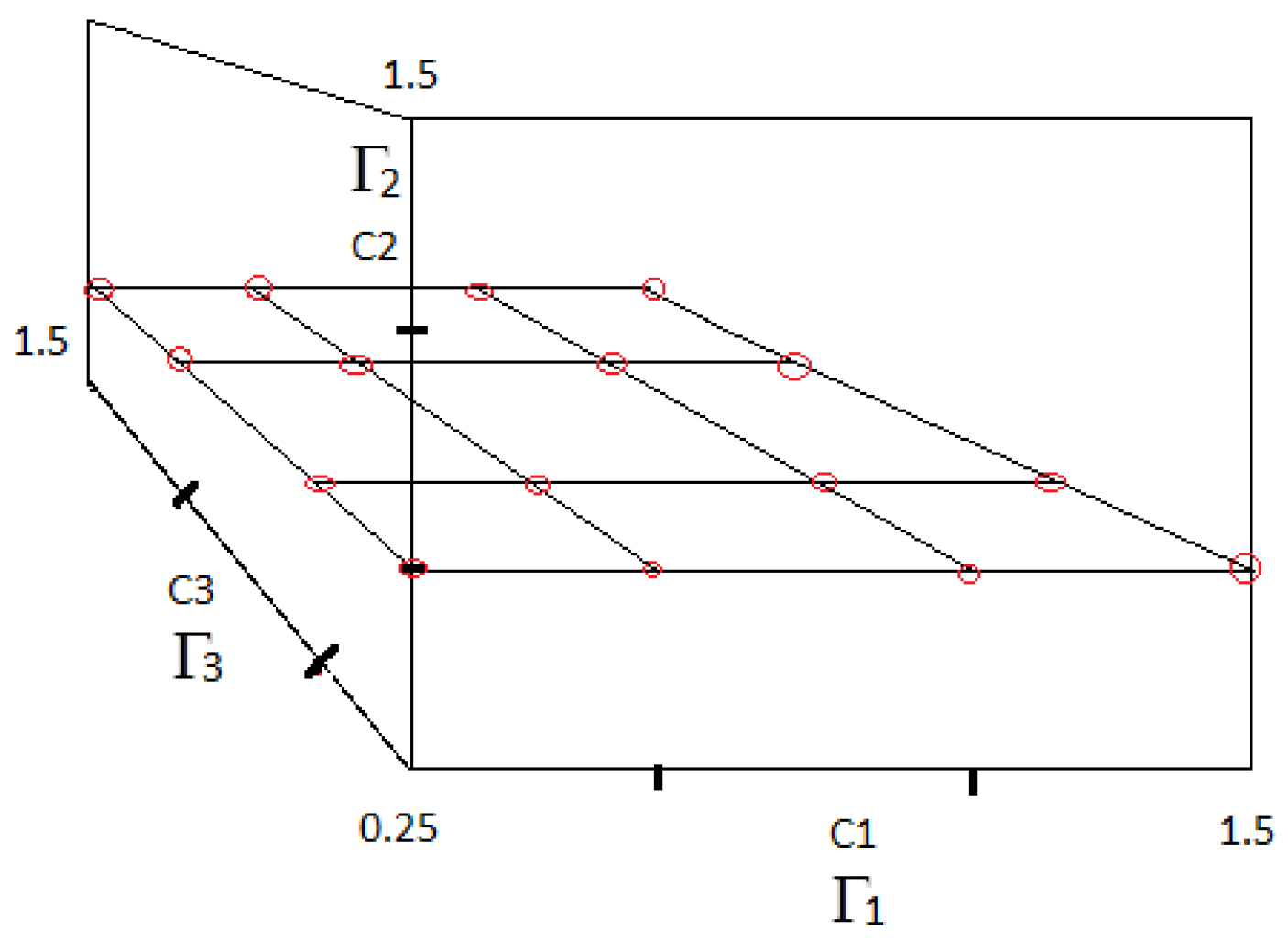
The next step after the first bunch of start points are created is to move on to the next plane along of the cuboid, as demonstrated in Figure 7. For this new fixed value of , the next set of start points is gathered along the grid generated on this section plane of the cuboid. These points are again clearly demonstrated in Figure 7 via the red encirclements. The idea is to continue the trend along the remaining subsequent sections of the cuboid for different values of until the start points from the final top layer are extracted. Hence, by using such an approach, all possible combinations of controller locations are generated from all over the function space. For a higher number of controllers in the higher dimension, the same method is to be extended to the corresponding hypercube to gather all necessary start points for the multi-start optimization procedure. With the example procedure outlined above, a total of start points is finally generated.
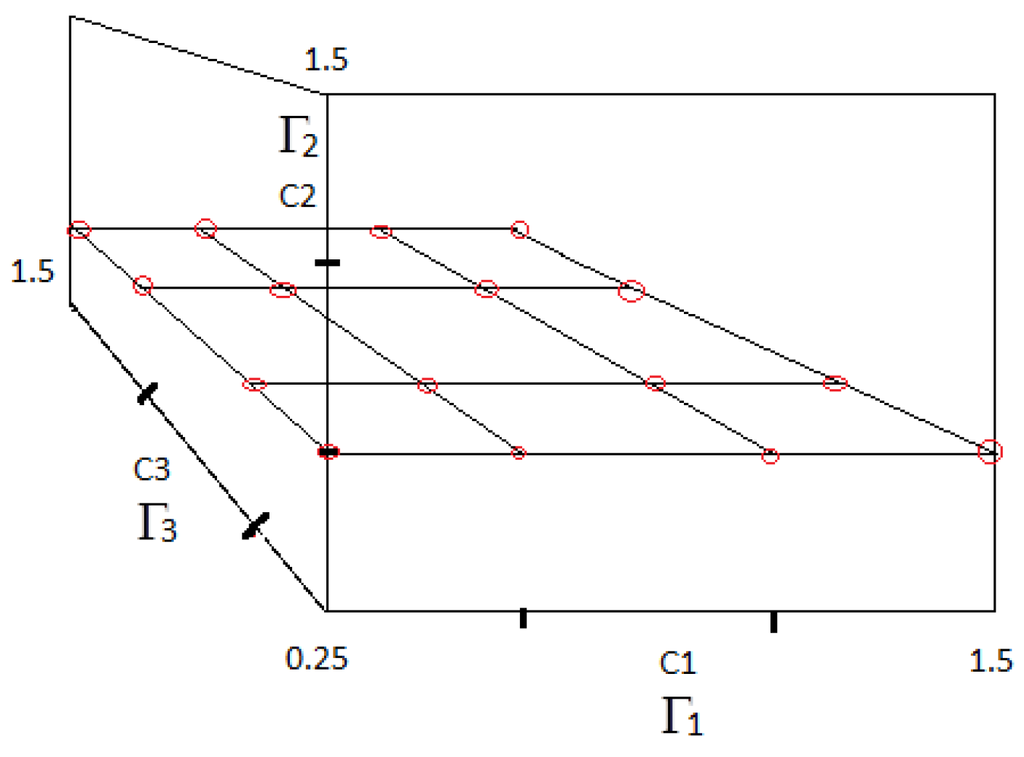
Figure 7.
Generation of start points: generated start points from the intermediate plane of the cuboid.
5.2. Minimization of MUASSC Structural Index: Reduction of Start Points
A set of start points encompassing the entire function space is now available from which one may begin individual optimization routines. It is theorized that the start points generated would be located within the cones of various minima, and hence, one can expect to arrive at them, following which, the best one is chosen.
However, as R, N increase, the number of start points grows in an aggressive manner, and therefore, due to the curse of dimensionality, performing individual optimization routines for all of the start points requires an extremely long time. Hence, to reduce such a burden, the next step in the method developed aims at rejecting start points that are deemed unnecessary due to a special structure that exists within the problem. One can take advantage of such a structure to finally arrive at a minimal set of start points for which individual optimization routines may be performed. The illustration of such rejections is as follows.
The reader is asked to consider such a situation where two controllers are placed at the same location of the uncertainty. This gives rise to redundancy and is therefore undesirable. Hence, the small number of start points that satisfies such a combination type are rejected from the list. Moreover, due to such a placement scheme, in most cases, the complete uncertainty does not get stabilized, and β becomes infinity. Consequently, such a start point would be of no use due to its inability to move around because of its infinite initial value.
One can also expect a small number of start points, which are of the kind where all of the controllers are placed at the same location in the uncertainty set. This is a case where the redundancy is even higher as compared to the previous situation, and the entire purpose of a “multi-model” scheme is lost. Hence, such kind of start point is also subtracted from the list of viable initial conditions. Most certainly, in almost all cases, such a combination will lead to a case of β being infinity.
One can also imagine a situation wherein although the controllers are placed at distinct locations, the effective set covering is insufficient, thereby leading to another case where β becomes infinity. All such start points that have a corresponding β of infinity, can be effectively rejected from the remaining list of start points. Such a form of rejection is effective at filtering out a significant amount of start points.
Another form of analytical rejection scheme has been identified, which is responsible for a massive reduction in the number of initial start points. It is clear that irrespective of the sequence of controller placements, as long as the location for all controllers remains constant, the value of β obtained also remains a constant. For instance, one may deduce the situation where the combination of yields the same value of β as , which in turn produces the same value of β for . Hence, for every combination of controller locations, all permutations lead to the same value of β. Therefore, the next step in the process of start point rejections is to retain only one permutation and eliminate the rest. In the case of , permutations exists out of which any five can be rejected. In cases with a higher number of controllers, this plays a very significant role, as for example, for , permutations would exist, out of which 119 can be rejected.
The combined effect of all stated methods is expected to significantly cut down the number of initial start points generated for the optimization process. In the next section, a graphical perspective of the aforementioned rejection method is presented. This provides a clear picture of how such rejection schemes work successfully to narrow down the regions of function space where minima may exist while tackling discontinuity and non-linearity.
5.3. Graphical Representation of Start Point Rejections
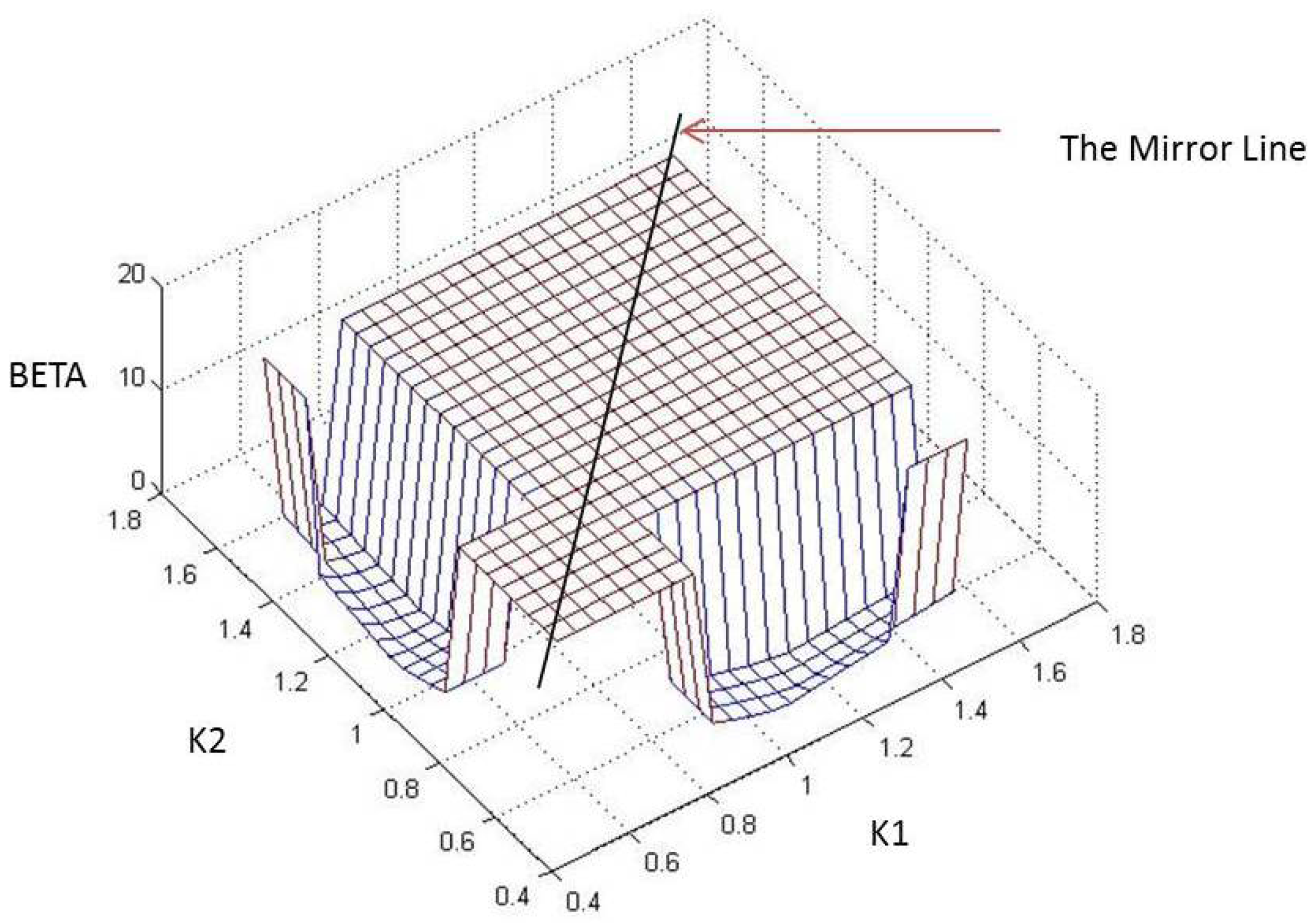
To provide a visual impression of the variation of β with controller locations, the initial set of has been shrunk to , such that at least two controllers are capable of stabilizing the entire uncertainty. Hence, with and placed at varying locations along the x and y coordinates, the corresponding β is plotted on the z axis as in Figure 8. For demonstration purposes, from Figure 9, Figure 10 and Figure 11, locations where actually correspond to the case where , but has been fixed at 20 to aid in the visualization. From Figure 8, also notice the discontinuous and non-linear nature of the cost function to be minimized.
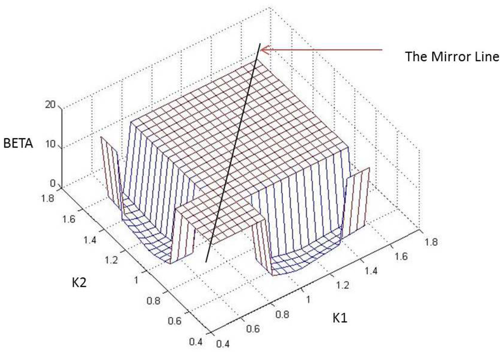
Figure 8.
Graphical representation of β variation with controller locations.
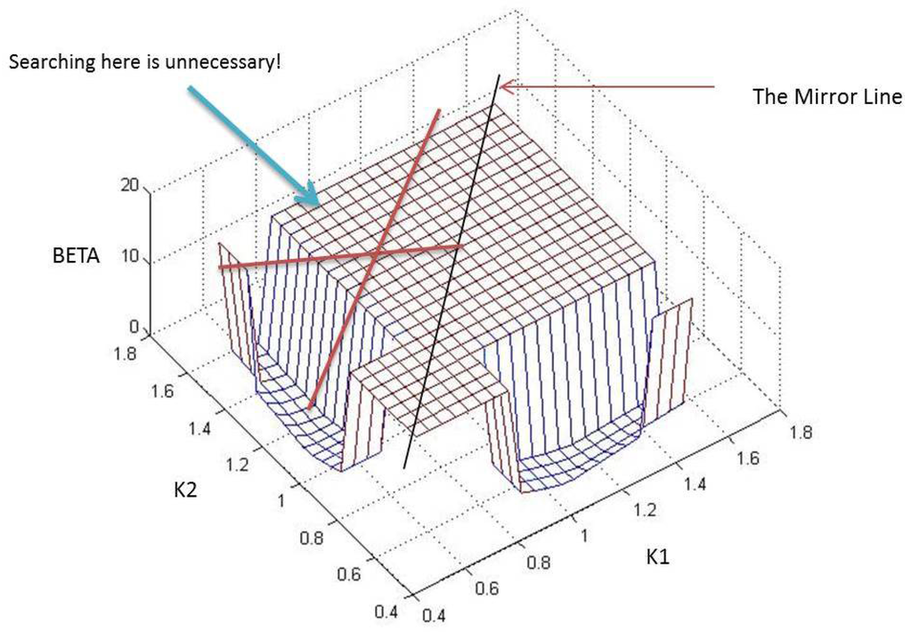
Figure 9.
Mirrored space rejected.
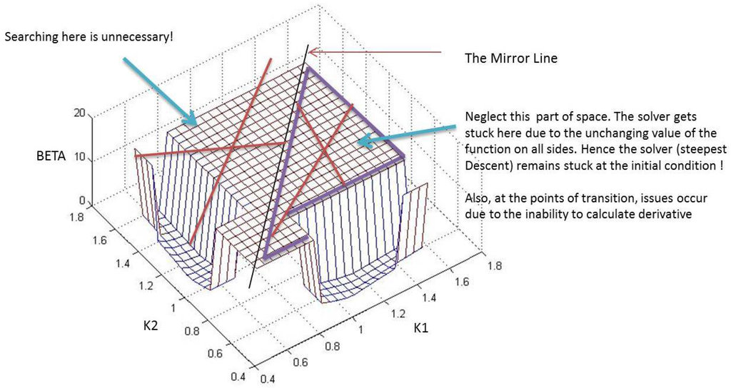
Figure 10.
Space with rejected.
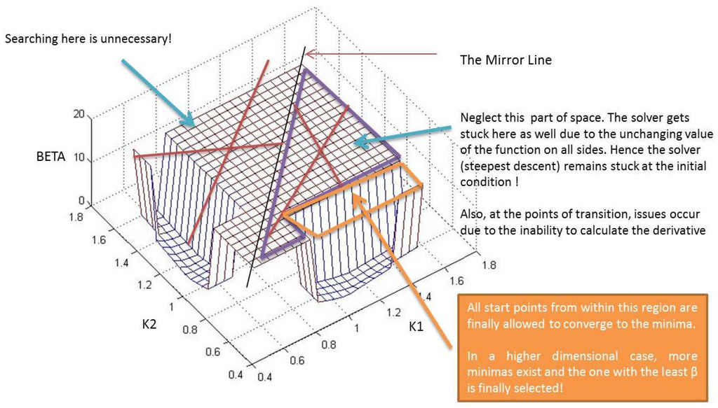
Figure 11.
Final space containing chosen start points.
From the previous discussion, it was shown that for a given combination of controller locations, all different permutations of controller placements ultimately lead to the same β value. For instance, from Figure 8, it is clear that the β obtained for is equal to the one obtained for the permutation . Similarly, for example, β for is the same as . Hence, it is inferred that a part of the function space mirrors the other, and hence, searching in only one part for the minima should suffice. This is clearly demonstrated in Figure 9 where the “Mirror Line” divides the space (for the 2D case) into two parts. Such a situation gets extended into higher dimensions upon the addition of more controllers. By rejecting all but one permutation of controller location combinations, one is essentially removing all start points that lie in these “mirrored” or redundant parts of the function space. This form of rejection for the 2D case has been clarified through Figure 9.
Next, upon removal of the previous start points, all such points starting within the section where (equal to 20 in Figure 8, Figure 9, Figure 10 and Figure 11) are also removed. As shown in Figure 10, any attempt to begin from such a location is futile, as there will not be any movement of the solver due to the flatness of the space all around. Furthermore, at points of transitions where β jumps to ∞ from a finite value, the solver might get stuck owing to the fact that the derivative cannot be calculated at such locations. This process has been clearly laid out in Figure 10. Finally, as shown in Figure 11, all start points that originate within the orange box are allowed to converge to the minima. In the case presented, only one such minimum exists within the orange boundary, but in higher dimensions, more such minima might. After the set of minima are chalked out, the location configuration corresponding to the least β among all obtained is finally selected. The next section describes the optimization procedure adopted along with the example of the three controller case.
5.4. Optimization Procedure with an Example of the Three Controller Case
The previous section dealt with the selection of only a section of start points from the initial list generated. Next, from the remaining start points, an optimization procedure using the steepest descent algorithm is applied to arrive at minima (other kinds of optimization algorithms can be found, for instance, in [20,21]). From the list of minima attained, the corresponding value of β, which is least among all, is selected. Once this value is attained, the procedure is augmented with a final step. In the most optimal case, the location of the β occurrence in the uncertainty set is analyzed. If this occurred at the edge of the uncertainty, then the controller closest to the boundary is posed as the design variable of a final optimization routine, while the rest are kept constant. This is done to further attain a more-optimal minimum if possible.
Alternatively, if β occurred in such a location, such that two controllers exist on either side of it, then both of these controllers are individually posed as design variables of two distinct optimization problems, which are allowed to run one after the other for the reason above. The result of the first is used as the initial condition for the next, and hence, it is necessary to perform said minimization in the above sequence.
The complete process of start point generation, rejection and optimization was carried out for the previously presented case of and for the same uncertain set of . The procedure was carried out with a grid resolution value of . Hence, as the number of start points that were obtained are start points. After performing the start point removal process, only 56 points were left (reduction of ) from which separate optimization procedures were started, following which, 14 distinct minima were arrived at. After the first round of optimizations, the best controller location combination that yielded the least β was with a corresponding value of . After the second round of optimization (i.e., the controllers on either side of β were individually used for optimization), the value of β further declined to for the locations of . The result was approximately lesser than the previous obtained for the original three controller configuration of . Hence, the process of individually performing two levels of optimization did indeed aid the process of arriving at the best possible optima. With a greater grid resolution of and , the number of minima remained at 14, thereby providing an indication that the ability to find more hidden minima with increased grid resolution R has been exhausted. Increasing R after this will have minimalistic effect on the number of minima found.
5.5. Decision of N-Number of Controllers for Uncertainty
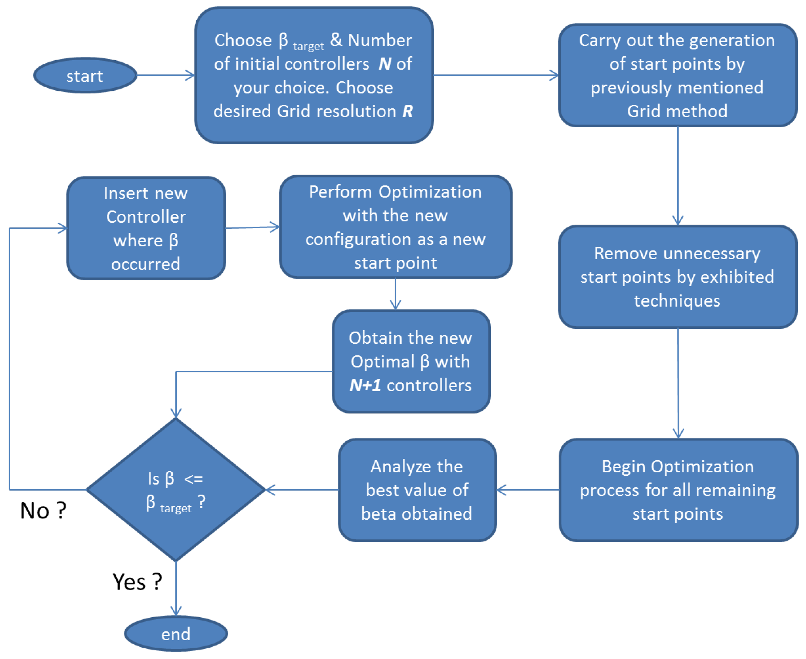
The previous methods are applicable once the number of controllers N has been decided. Consequently, the next question to be asked is how can one decide this in the first place? This section presents a way to introduce the choice of N and integrates it with the optimization procedure above. The crucial idea is to fix a target and the “number of initial controllers that the reader feels might work” and then performing the mentioned procedure to yield the best β. If this is greater than the target, N is increased by one, and the new controller is placed at the location where the previous best β occurred. The new obtained controller combination (now with one extra controller) is used as the start point for another two-step optimization routine to obtain the new β, which is then compared to the target. If , then one may stop or else the same procedure is repeated till the condition is satisfied. Refer to Figure 12 for a step by step flowchart of the procedure. For the example uncertainty set of , the least value of N was three itself.

Figure 12.
Flowchart of Algorithm 1.
A major drawback in the scheme above is that once a new controller is added at the location of β occurrence, the new combination is used as a start point for a similar two-step minimization procedure. This is risky, as the new start point might lie in the cone of a local minima in the next dimension. Hence, an alternative procedure is suggested, wherein if after the first cycle, the best β fails to attain the target, the N is increased by one, and once again, the complete cycle of grid generation, start point reduction and multi-start optimization is performed (now for controllers) to obtain the globally least β. This process can go on till the target is achieved. This is clear from the flowchart in Figure 13. An example to demonstrate the optimality of the second scheme as compared to the first is as follows:
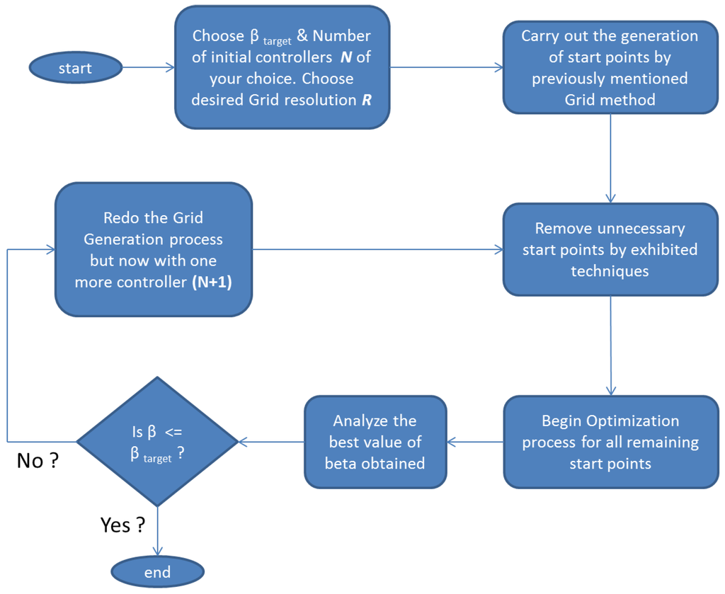
Figure 13.
Flowchart of Algorithm 2.
The was set to for an uncertainty set of with the initial guess of the number of controllers N being two. By using Scheme 1, the most optimal value of β obtained was for three controllers, whereas on the contrary, upon utilizing Scheme 2, the optimal was . Hence, the issue occurred in the first case when N was increased to three; the new controller was inserted where β for occurred, which in turn was in the cone of a sub-optima. This issue gets circumvented if the multi-start process is repeated once again, which is precisely what Scheme 2 introduces. Of course, there is a trade-off of greater computational requirements in the latter. It is to be noted that the norm is continuous with respect to the parameter changes that occur. A further improvement to the present method is where once the appropriate function space for the minima has been identified, one may use genetic algorithms or subgradient-based methods to improve the search time. The new scheme as outlined above is a new approach towards answering the posed question in the section on research goals.
6. Improving the RMMAC Structural Index
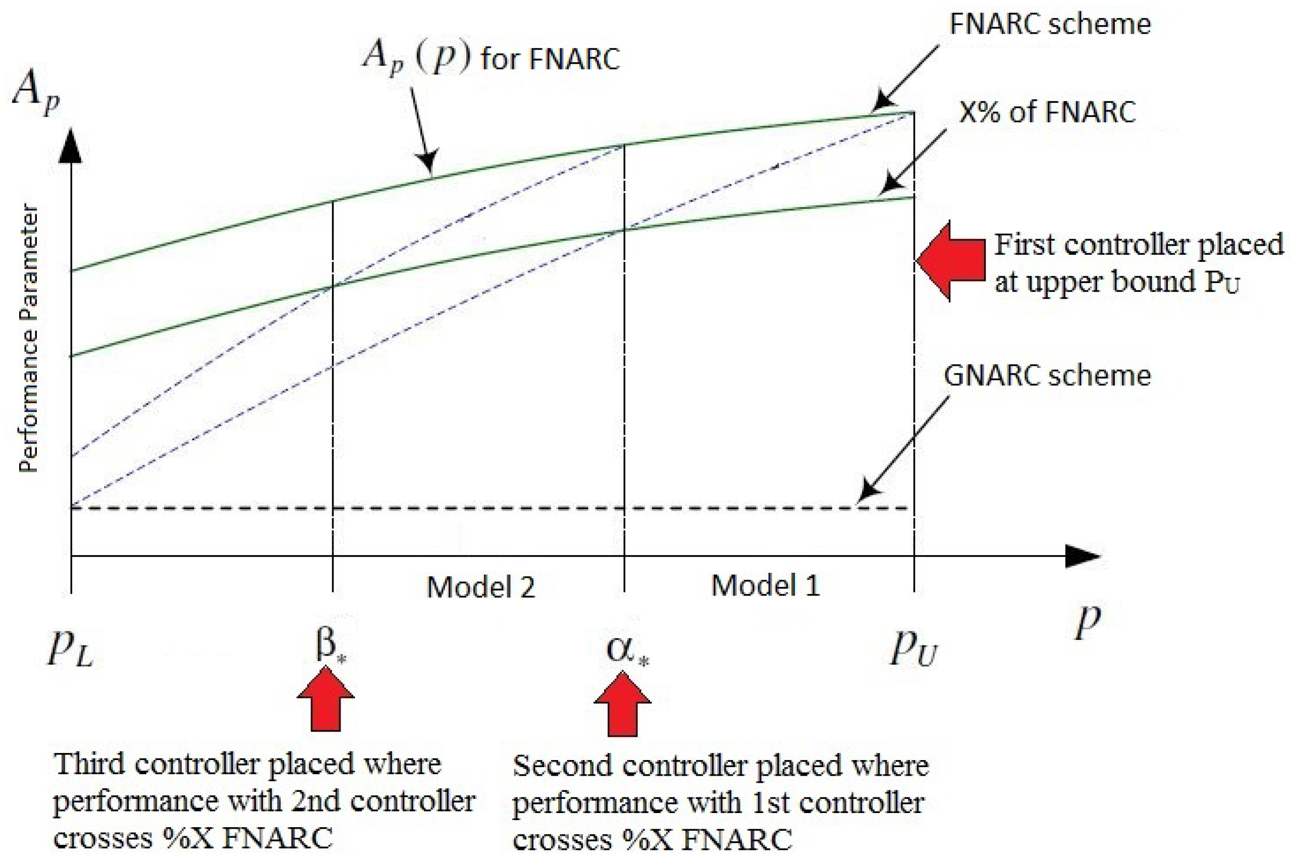
To introduce the the RMMAC structural index, the reader is referred to Figure 14. The green plot denotes the best possible performance with the FNARC infinite controller scheme. The of FNARC line denotes a fraction () of the best possible FNARC performance and, hence, follows a similar trajectory. It is to be noted that in the RMMAC case, the performance variable is essentially one over the mixed sensitivity peak for that specific plant/controller combination, as opposed to using the mixed sensitivity peak directly, as done in the MUASSC case. This alternate method proposes that the first controller be placed at the upper bound of the uncertainty. In Figure 14, and denote the upper and lower bounds of the given uncertainty. Once the first controller is placed at , the degradation in performance is tracked as the true parameter moves away from with the dotted blue line. is the location where this degraded trajectory crosses the of the best possible performance. The value of is the performance degradation tolerable by the user as compared to the best possible FNARC case. Hence, the method proposes that at , a second controller is placed where the performance jumps up again to become equal to the FNARC case, with its degradation being tracked once more. Wherever this crosses the FNARC trajectory, in this case , again, a new controller is placed. This process in continued till the entire set is stabilized and guarantees a performance equivalent to of FNARC at the least.
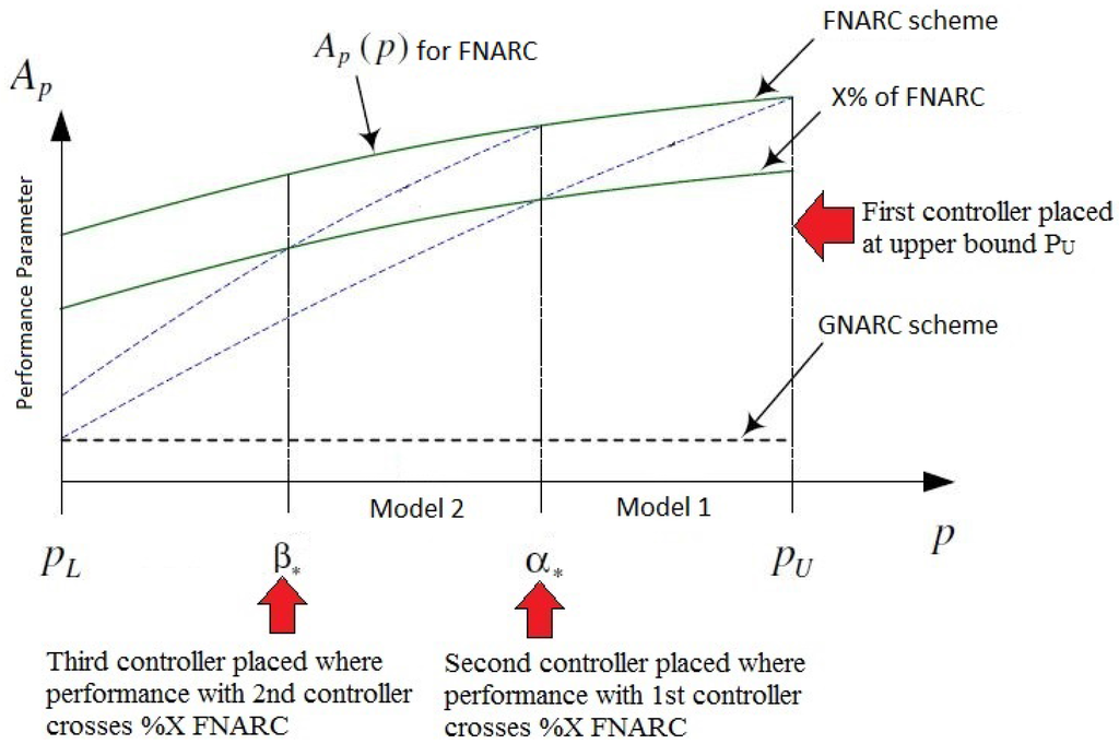
Figure 14.
Structural index selection in RMMAC [7].
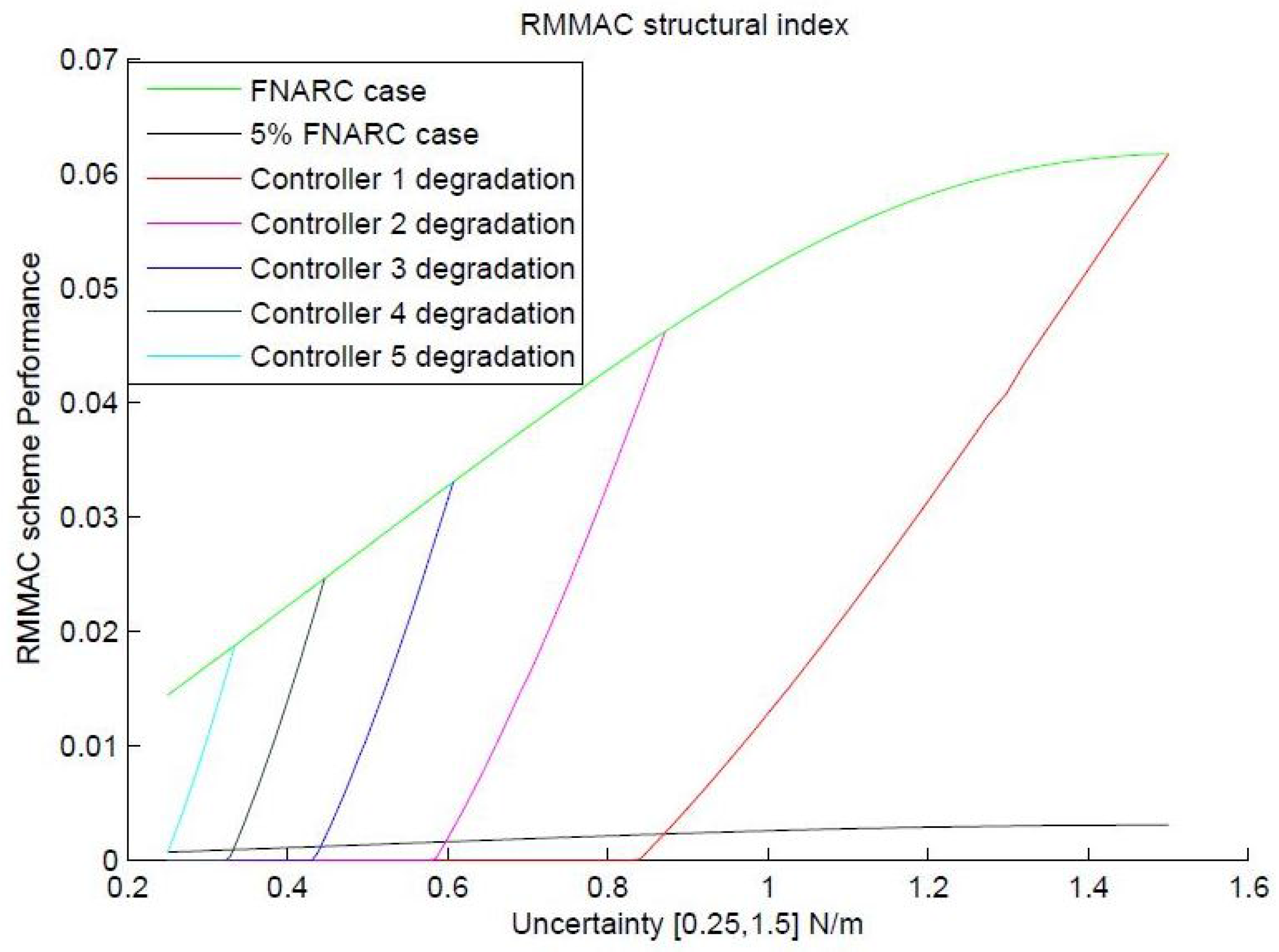
The placement scheme was tried out with the classic uncertainty of , and the results were inspected. For an of just , according to the scheme, at least five controllers placed at are required to stabilize and guarantee performance for the whole set as opposed to just three controllers (with and locations ) suggested by the new method introduced before. The placement of controllers in the RMMAC case has been visually demonstrated in Figure 15 for clarity. A corresponding beta value of was obtained for the controller placed using the RMMAC scheme with locations of . In parallel, the scheme introduced in the previous sections was used to decide the controller locations for a fixed , which subsequently gave a result of for the locations of . Clearly, the value of β synthesized using the novel technique is lower and, hence, presumed to provide superior transient performance according to Theorem 1. In the next section, extensive simulations have been performed using the MUASSC scheme to validate the claimed optimality by comparing the controller locations suggested by the RMMAC structural index with the controller locations suggested by the MUASSC optimal structural index method of β minimization. A fact to be noted in the RMMAC structural index scheme is that the controller placement locations take into account the final mixed sensitivity performance with the best controller switched on, but lack the guarantee that the best controller will be turned on in the first place, if the above RMMAC scheme of probabilistic mixing is replaced by a switching mechanism selecting only one controller at a time.

Figure 15.
RMMAC scheme with uncertainty of .
Suggestion to Improve the Structural Index of RMMAC
The reason the method suggests a greater number of controllers is the initial suboptimal placement of the first controller at the upper bound directly. A controller is capable of handling uncertainties on either side, and hence, all of the plant values that Controller 5 in RMMAC could have handled on its right are not part of the set anymore. Hence, an intelligent tweak has been suggested wherein the last controller is shifted inside the set, and this location is decided by again charting the degradation of the first controller on either side. To make this simpler, the reader is referred to Figure 16. As shown in the figure, the first controller is placed intelligently (at ), such that it is allowed to tackle uncertainty on either side, while guaranteeing stability and performance that is at least of the best possible FNARC performance. Once the first controller is placed, the rest of the process is the same. Clearly, with the added tweak, the number of controllers has reduced to four, and they are placed at instead of the previously suggested five.
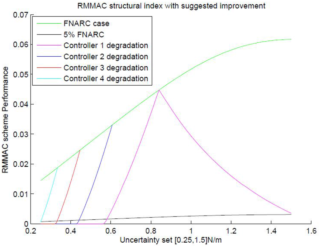
Figure 16.
Modified RMMAC scheme with uncertainty of .
7. Results
The algorithms to optimize β are put to test, and it is checked whether the value of the MUASSC structural index is actually reduced. As briefly mentioned during the section that introduces the algorithm of β minimization, the first comparison was done with three controllers making up the controller bank. It is to be noted that the controller bank mentioned here corresponds to the one that is put in feedback with the original spring mass plant example that has been introduced in Section 4. Hence, the unknown parameter corresponds to the stiffness of the spring between the two masses and therefore has as its unit. Initially, for the MUASSC case, the controllers were synthesized corresponding to , which produced a value . After running the algorithms developed above, the suggested locations were with a corresponding . Definitely, this is a reduction, and a similar comparison was done with five controllers making up the controller bank. As the previously-suggested RMMAC structural index methodology requires a minimum of five controllers to be placed at , this becomes the basis of comparison for the five controller case. After calculating β for this combination, a value of was yielded. Next, keeping , the above developed algorithm was applied, and subsequently, the β for the resulting combination was evaluated. Like the case of , here too, the value of β reduced, with the suggested location for controller placement being , which yielded a value of . Hence, the developed methodology reduced the value of the yielded β for both cases of , as well as .
For the benefit of the reader, the combination of spring stiffnesses where the controllers were placed and the corresponding β obtained are summarized in Table 1. To conclude, this viable method proposed aims to minimize the introduced variable β using a multi-start minimization approach coupled with intelligent techniques of contracting the search space drastically. The corresponding tuning variables are the controller locations, and it is hypothesized that the locations corresponding to the lowest possible β are the best possible controller locations. This method was coupled with a way of determining the number of controllers for a given uncertainty where two different possible methods were suggested. The second method bypasses the possibility of getting stuck in a local minima, when N is increased, but comes at a cost of higher computational requirement.

Table 1.
β with different controller combinations.
It has been demonstrated that the minimization mechanism introduced through this work was indeed successful in reducing the value of β. Simulations must be now performed to prove that minimizing β did indeed lead to an improved performance in the MUASSC scheme. Two points of comparison that have been identified are the greatest switching time and the number of switches. The greatest switching time indicates the highest time it took for the correct controller to be turned on for varying values of spring stiffness in the uncertainty set, while the number of switches indicates the total switches that occurred before the most appropriate controller was placed in the loop by the supervisor. The simulations were compared between the initial and optimal configurations in the three (original MUASSC vs. optimal MUASSC), as well as the five controller (original RMMAC vs. optimal MUASSC) case. The results of the simulations are presented in Table 2 and Table 3. Once again, the aforementioned MUASSC simulations were carried out with the same spring mass plant configuration that has been previously introduced. The aforementioned performance criteria were analyzed for this plant with the various controller configurations.

Table 2.
Performance comparison for the 3 controller case.

Table 3.
Performance comparison for the 5 controller case.
Author Contributions
S.B. conceived and designed the experiments; D.G. performed the experiments; S.B. and D.G. analyzed the data; D.G. wrote most of the paper.
Conflicts of Interest
The authors declare no conflict of interest.
References
- Hespanha, J.P.; Liberzon, D.; Morse, A.S. Overcoming the limitations of adaptive control by means of logic-based switching. Syst. Control Lett. 2003, 49, 49–65. [Google Scholar] [CrossRef]
- Baldi, S.; Battistelli, G.; Mosca, E.; Tesi, P. Multi-Model Unfalsified Adaptive Switching Supervisory Control. Automatica 2013, 46, 249–259. [Google Scholar] [CrossRef]
- Baldi, S.; Battistelli, G.; Mosca, E.; Tesi, P. Multi-model unfalsified adaptive switching control: Test functionals for stability and performance. Int. J. Adapt. Control Signal Process. 2013, 25, 593–612. [Google Scholar] [CrossRef]
- Baldi, S.; Battistelli, G.; Mosca, E.; Tesi, P. Multi-model unfalsified switching control of uncertain multivariable systems. Int. J. Adapt. Control Signal Process. 2013, 26, 705–722. [Google Scholar] [CrossRef]
- Baldi, S.; Ioannou, P.; Mosca, E. Evaluation of identifier based and & non-identifier based adaptive supervisory & control using a benchmark example. In Proceedings of the 2010 4th International Symposium on Communications, Control and Signal Processing (ISCCSP), Limassol, Cyprus, 3–5 March 2010; pp. 1–6.
- Baldi, S.; Battistelli, G.; Mari, D.; Mosca, E.; Tesi, P. Multi-model adaptive switching control with fine controller tuning. In Proceedings of the 18th IFAC World Congress, Milano, Italy, 28 August–2 September 2011; pp. 374–379.
- Fekri, S.; Athans, M.; Pascoal, A. Issues, progress and new results in robust adaptive control. Int. J. Adapt. Control Signal Process. 2006, 20, 519–579. [Google Scholar] [CrossRef]
- Narendra, K.S.; Balakrishnan, J. Improving Transient Response of Adaptive Control Systems using Multiple Models and Switching. IEEE Trans. Autom. Control 1994, 39, 1861–1866. [Google Scholar] [CrossRef]
- Angeli, D.; Mosca, E. Lyapunov-Based Switching Supervisory Control of Nonlinear Uncertain Systems. IEEE Trans. Autom. Control 2002, 47, 500–505. [Google Scholar] [CrossRef]
- Narendra, K.S.; Balakrishnan, J. Adaptive control using multiple models. IEEE Trans. Autom. Control 1994, 42, 171–187. [Google Scholar] [CrossRef]
- Stefanovic, M.; Safonov, M.G. Safe Adaptive Switching Control: Stability and Convergence. IEEE Trans. Autom. Control 2008, 53, 2012–2021. [Google Scholar] [CrossRef]
- Safonov, M.G.; Tsao, T.C. The Unfalsified Control Concept and Learning. IEEE Trans. Autom. Control 1997, 42, 843–847. [Google Scholar] [CrossRef]
- Baldi, S.; Ioannou, P.A.; Kosmatopoulos, E.B. Adaptive mixing control with multiple estimators. Int. J. Adapt. Control Signal Process. 2012, 26, 800–820. [Google Scholar] [CrossRef]
- Hespanha, J.P.; Liberzon, D.; Morse, A.S. Hysteresis-based switching algorithms for supervisory control of uncertain systems. Automatica 2003, 39, 263–272. [Google Scholar] [CrossRef]
- Kwakernaak, H. Robust Control and H∞ Optimization Tutorial Paper. Automatica 1993, 29, 255–273. [Google Scholar] [CrossRef]
- Hingane, A.; Sawant, S.H.; Chavan, S.P.; Shah, A.P. Analysis of Semi active Suspension System with Bingham Model Subjected to Random Road Excitation Using MATLAB/Simulink. IOSR J. Mech. Civil Eng. 2006, 3, 1–6. [Google Scholar]
- Chikhale, S.J.; Deshmukh, S.P. Comparative Analysis Of Vehicle Suspension System in Matlab-SIMULINK and MSc-ADAMS with the help of Quarter Car Model. Int. J. Innov. Res. Sci. Eng. Technol. 2013, 2, 4074–4081. [Google Scholar]
- Dowds, P.; O’Dwyer, A. Modelling and control of a suspension system for vehicle applications. In Proceedings of the 4th Wismarer Automatisierungs Symposium, Wismar, Germany, 22–23 September 2005.
- Lee, J.J. H∞ control of Flexible Structures. Master’s Thesis, University of Hawaii at Manoa, Manoa, HI, USA, 1997. [Google Scholar]
- Hestenes, M.R. Multiplier and gradient methods. J. Optim. Theory Appl. 1969, 4, 303–320. [Google Scholar] [CrossRef]
- Kelley, J.E. The cutting plane method for solving convex programs. J. SIAM 1960, 8, 703–712. [Google Scholar]
© 2016 by the authors; licensee MDPI, Basel, Switzerland. This article is an open access article distributed under the terms and conditions of the Creative Commons by Attribution (CC-BY) license (http://creativecommons.org/licenses/by/4.0/).

