Article

Dynamic Contact between a Wire Rope and a Pulley Using Absolute Nodal Coordinate Formulation

1
Department of Engineering and Applied Sciences, Sophia University, 7-1 Kioi-cho, Chiyoda-ku, Tokyo 102-8554, Japan
2
Department of Mechanical Engineering, Tokyo Metropolitan University, 1-1 Minami-Ohsawa, Hachioji-shi, Tokyo 192-0397, Japan
*
Author to whom correspondence should be addressed.
Machines 2016, 4(1), 4; https://doi.org/10.3390/machines4010004
Submission received: 27 June 2015 / Revised: 12 January 2016 / Accepted: 14 January 2016 / Published: 21 January 2016
(This article belongs to the Special Issue Advance in Multibody System Dynamics)

Abstract

:
Wire rope and pulley devices are used in various machines. To use these machines more safely, it is necessary to analyze the behavior of the contact between them. In this study, we represent a wire rope by a numerical model of a flexible body. This flexible body is expressed in the absolute nodal coordinate formulation (ANCF), and the model includes the normal contact force and the frictional force between the wire rope and the pulley. The normal contact force is expressed by spring-damper elements, and the frictional force is expressed by the Quinn method. The advantage of the Quinn method is that it reduces the numerical problems associated with the discontinuities in Coulomb friction at zero velocity. By using the numerical model, simulations are performed, and the validity of this model is shown by comparing its results with those of an experiment. Through numerical simulations, we confirm the proposed model for the contact between the wire rope and the pulley. We confirmed that the behavior of the wire rope changes when both the bending elastic modulus of the wire rope and the mass added to each end of the wire rope are changed.

1. Introduction

Wire rope and pulley devices are used in various machines, such as cranes and elevators [1]. As machine elements, they have various advantages, such as being lightweight, having a small footprint, and being useful in a wide variety of machines. In addition, ropes and cables can be used in extreme environments, such as in space and deep in the ocean. Cables are also used to attach satellites to a mothership [2,3] or to operate vehicles remotely. In each of these machines, pulleys are used to change the direction of the force and to transfer power. To ensure that these machines are used safely, it is important to consider the contact between the rope and the pulley. For example, if the friction between them is used to transfer power in an elevator system, slip is produced when there is a difference between the tension on the right side and that on the left side. When using a pulley in microgravity, deformation occurs where the rope is wound, and this can lead to fractures. To solve these problems, it is necessary to perform an advanced analysis of the contact between the rope and the pulley. However, most of the relevant research has been directed at the vibration of the rope [1,4,5] or the motion of the rope. Few studies have considered the contact between the rope and pulley [6], and those that have have been based on physical experiments [7], not on numerical simulations. Consequently, it is important to develop a numerical model in which the parameters can be changed and the deformations of the contacting parts can be evaluated.
The purpose of this study is to construct a numerical model that can use flexible multibody dynamics to investigate the motion of the contact part of the pulley and express in detail the normal contact and frictional forces between a rope and pulley. First, the validity of the model is shown by comparing the results with those of an experiment. We then use the numerical model to perform simulations under various conditions. We also examine the force acting between the wire rope and the pulley and the resulting motion. Additional simulations are performed in which various masses are added to each end of the rope, and the influence of the ratio of tension, which is the ratio of the weights applied to each end of the rope, and the bending elastic modulus of the wire rope are varied; we discuss the influence of each of these factors on the motion of the rope.

2. Modeling of Rope and Pulley

In this section, we discuss the formulation of the numerical model. The wire rope is modeled by the absolute nodal coordinate formulation (ANCF) [8,9], the contact force is modeled by spring-damper elements, and the frictional force is defined by the Quinn method.

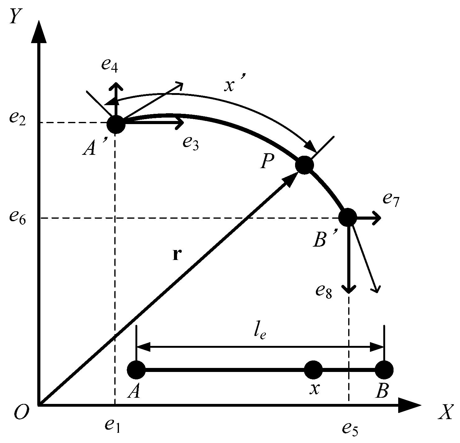
2.1. Formulation of Wire Rope

Using the ANCF to formulate the wire rope makes it easier to describe its motion as a flexible body with large deformation, large rotation, and large translational displacement. Figure 1 shows an element of a flexible body in the absolute coordinate system O-XY. Here, AB is the initial form, and A′B′ is the deformed form. The global position vector r of an arbitrary point on the element can be described by using the global shape function, as follows:
r = S e
The vector of the nodal coordinates is as follows:
e = [ e 1 e 2 e 3 e 4 e 5 e 6 e 7 e 8 ] T
where e1 and e2 are the positions at node A, e5 and e6 are the positions at node B, e3 and e4 are the spatial derivatives of the displacements of the node at A′, and e7 and e8 are the spatial derivatives of the displacements of the node at B′. In Equation (1), the following shape function is used:
S = [ S 1 S 2 ] = [ 1 3 ξ 2 + 2 ξ 3 0 0 1 3 ξ 2 + 2 ξ 3 l e ( ξ 2 ξ 2 + ξ 3 ) 0 0 l e ( ξ 2 ξ 2 + ξ 3 ) 3 ξ 2 2 ξ 3 0 0 3 ξ 2 2 ξ 3 l e ( ξ 2 + ξ 3 ) 0 0 l e ( ξ 2 + ξ 3 ) ] T
where ξ = x / l e , x is the coordinate along the body axis in the initial configuration, and l e is the length of the element. The kinetic energy in the flexible body element becomes
T = 1 2 0 l e ρ A r ˙ T r ˙ d x = 1 2 e ˙ T M a e ˙
Thus, an element mass matrix, expressed in terms of the global frame, becomes
M a = ρ A 0 l e S T S d x
Figure 1. Element of a flexible body.
Machines 04 00004 g001
Next, the strain energy is derived. A liner elastic model can be assumed by increasing the number of elements [10,11,12]. The longitudinal elastic potential energy of one element U l can be written as:
U l = 1 2 0 l e E l A ε 2 d x
where E l is the longitudinal elastic modulus, and ε is the axial strain of the element. The bending elastic potential energy of one element U t can be written as:
U t = 1 2 0 l e E b I κ 2 d x
where E b is the bending elastic modulus, I is the second moment of the area of the element, and κ is the curvature.
The equations of motion can be written as:
M e ¨ = Q f Q k
where M is the mass matrix, Q f is the external force, and Q k is the elastic force. Q k is defined as follows:
Q k = ( U l e ) T + ( U t e ) T
In this model, in order to express the characteristics of longitudinal strength and ease of bending, the modulus of longitudinal elasticity is different from the modulus of bending elasticity.

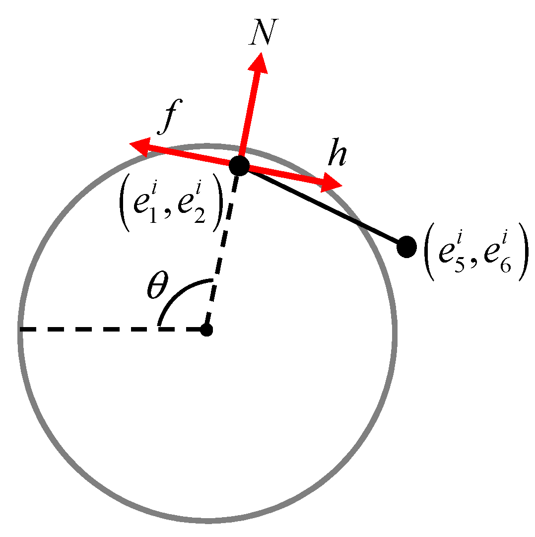
2.2. Formulation of Normal Contact Force, Frictional Force, and Constraint Force

The normal contact force is expressed by the spring-damper elements, and the frictional force is expressed by the Quinn method [13]. The advantage of the Quinn method is that there is a discontinuity, and so the Coulomb friction is consistent [14,15]. First, we formulate the normal contact force. Figure 2 shows the i-th element on which the normal contact and frictional forces act. The normal contact force acts when the node of an element has a boundary condition, and this depends on the radius of the pulley [16]. The i-th nodal coordinates are e 1 ( i ) , e 2 ( i ) . The radius of the pulley is R , and the coordinates of the center of the pulley are R x , R y . The boundary condition is
( R x e 1 ( i ) ) 2 + ( R y e 2 ( i ) ) 2 R 2
Figure 2. Forces acting on a rope.
Machines 04 00004 g002
The normal contact force is defined as normal to the pulley. The penalty parameter of the pulley is k c , the damping constant of the pulley is c c , the velocities of the i-th element are e ˙ 1 ( i ) , e ˙ 2 ( i ) , and d is the distance between the center of pulley and the i-th element. Hence, the normal contact force is
N = k c ( R ( R x e 1 ( i ) ) 2 + ( R y e 2 ( i ) ) 2 ) c c ( e ˙ 1 ( i ) cos θ + e ˙ 2 ( i ) sin θ )
cos θ = e 1 ( i ) R x d , sin θ = e 2 ( i ) R y d
Next, the frictional force is shown. The frictional force of the Quinn method is defined by the velocity and force acting on the nodal coordinate. The advantage of this method is that it reduces the numerical problems associated with the discontinuities in Coulomb friction at zero velocity, and, as a result, we can perform a numerical simulation at v ¯ = 0 , which is when slip-stick behavior plays a central role. The frictional force in Equation (13) is based on the total force h , which is a combination of the elastic force and the gravity acting on the i-th element, the velocity in the tangential direction v , the circumferential velocity of the pulley v p , the normal contact force N , a fixed regularization parameter ε [13], and the friction coefficient μ :
F ( v ¯ , h ) = { μ N v ¯ / ε sgn ( v ¯ ) μ N i f | v ¯ | ε o t h e r w i s e
v ¯ ( v , h ) = { v v p + ε h / μ N v v p + sgn ( h ) ε i f | h | μ N o t h e r w i s e
Finally, the two constraint forces are defined: In the longitudinal direction, there is a damping force on the edges of the rope; in the lateral direction, there is s constraint force on the edges of the rope. The normal contact force N , the frictional force F , and the constraint force depend on time. The contact between the rope and pulley is expressed by adding Qf as the external force in Equation (8).

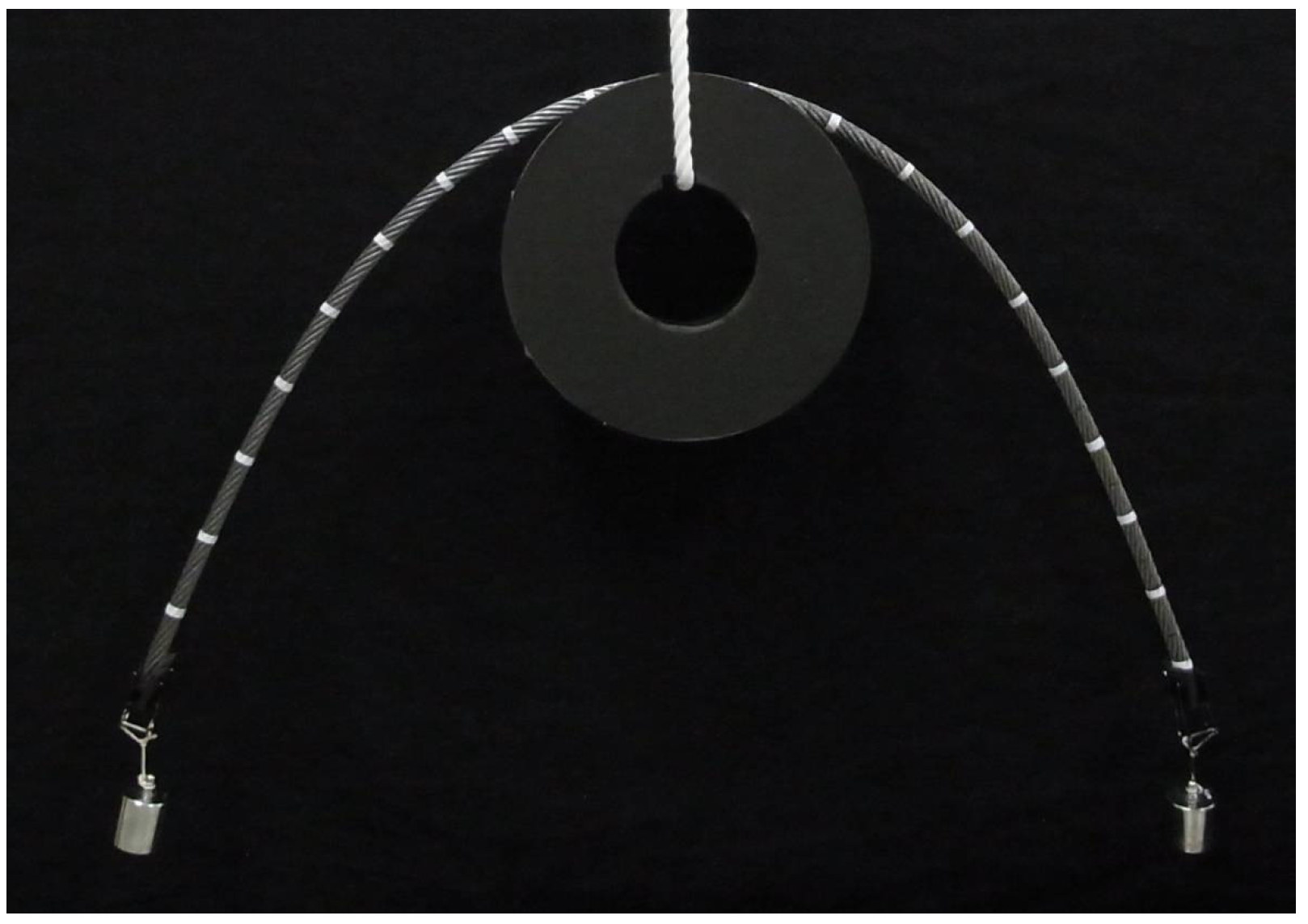
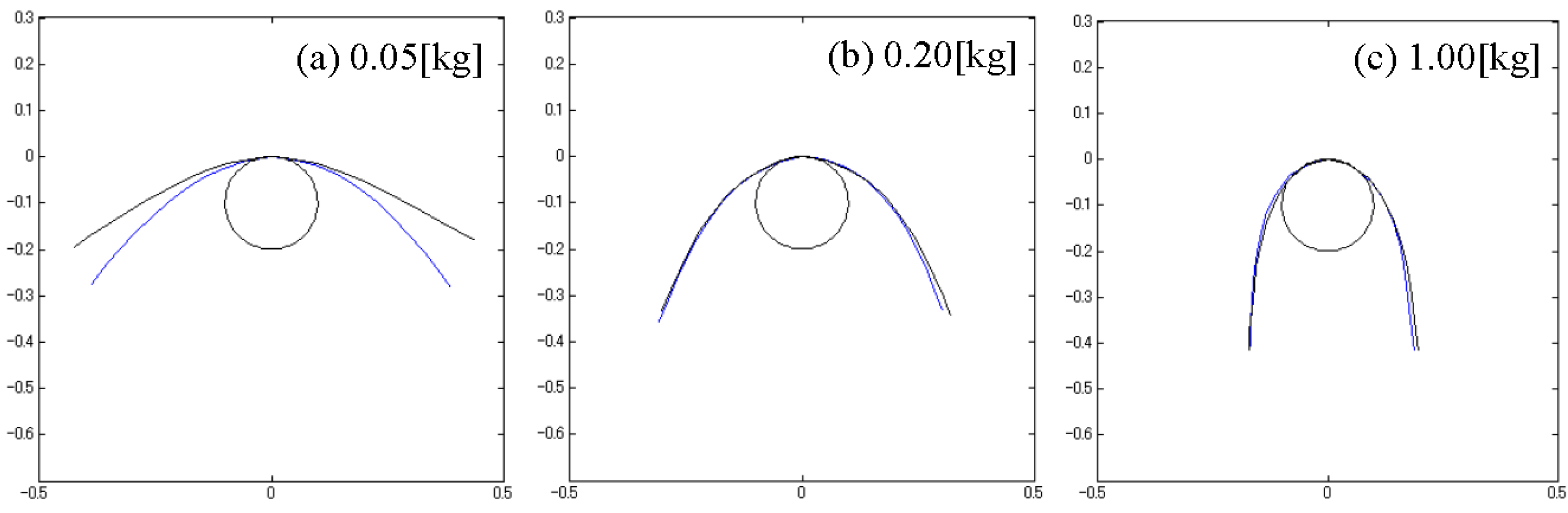
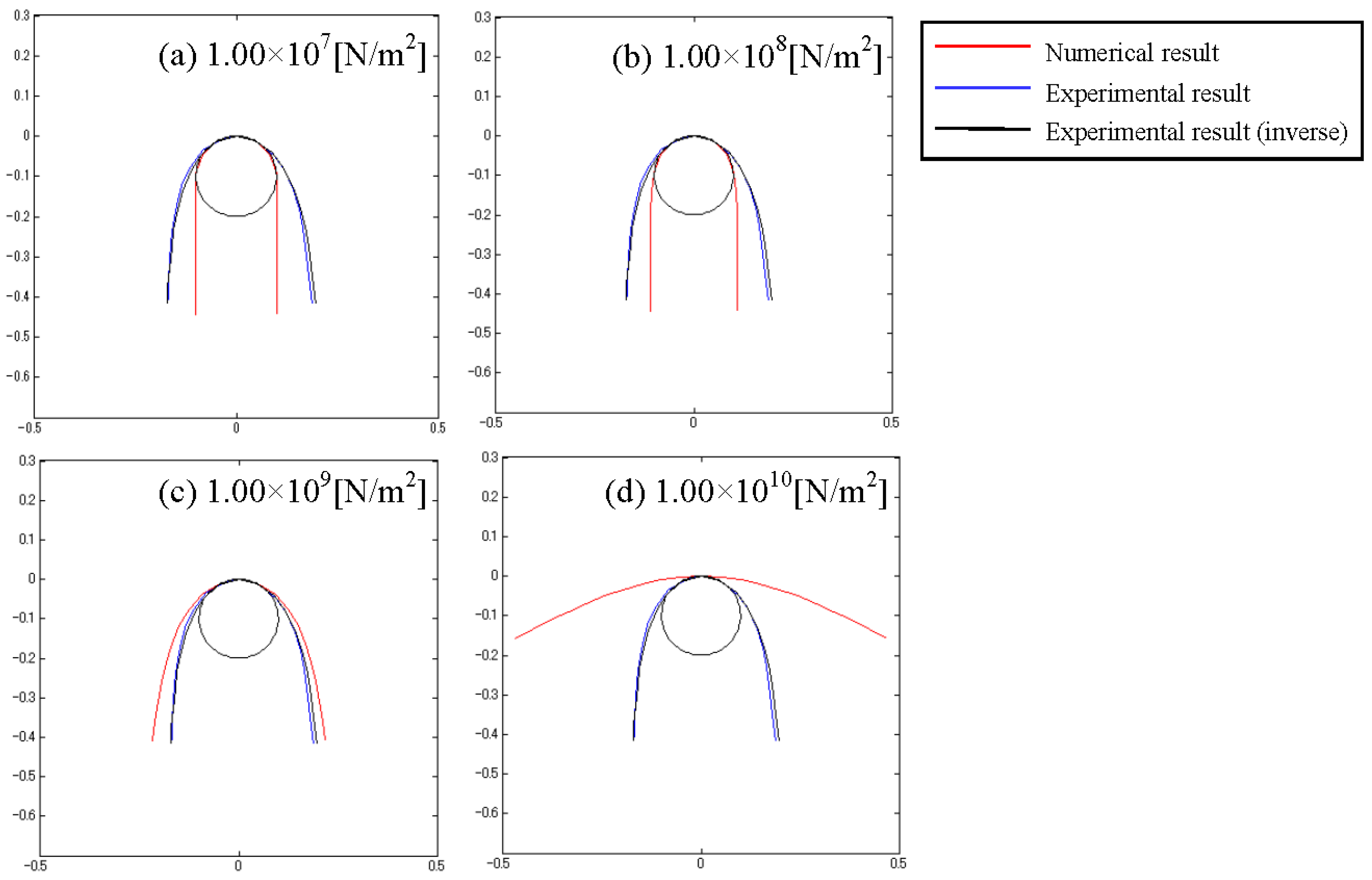
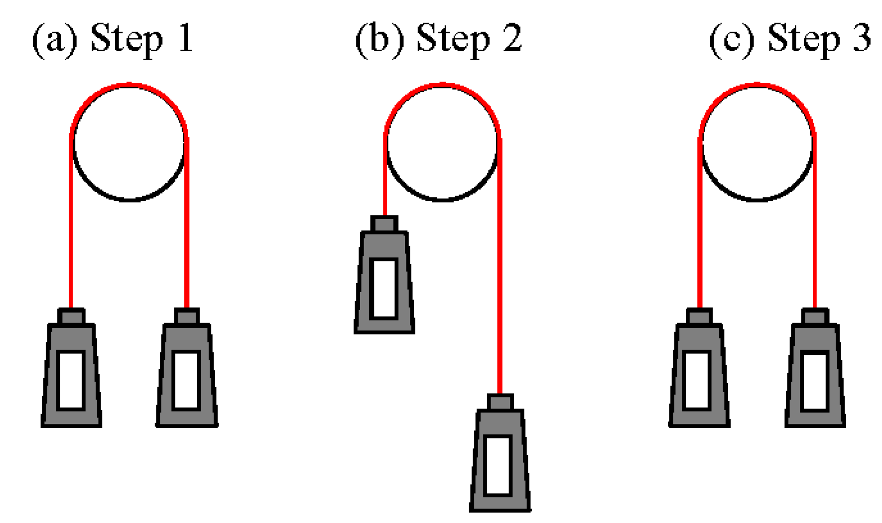
3. Validation of Numerical Model

In this section, we present the results of an experiment that we conducted to validate the results of the proposed model. The coefficient of longitudinal elasticity is specified, but the bending elastic modulus is not referred to in general. The coefficient of bending elasticity was determined by comparing the experimental and simulation results for the shape of a wire rope. In this process, the bending elastic modulus was treated as an unknown parameter. A fundamental experiment was performed to measure the shape of a wire rope used with a pulley. In this experiment, the wire rope had a length of 1.00 m and a diameter of 0.01 m. Weights of 0.05 kg, 0.2 kg and 1.0 kg were then added to each end of the wire rope, and a digital camera was used to determine their influence on the shape of the rope. Markers were placed on the wire rope at intervals of 0.05 m, and the displacement of the markers was calculated by using the graphics software package ImageJ [17,18] to analyze the photographs; this displacement was then used to determine the shape of the rope. Various masses were used. The wire rope was not straight, even when there is no load on it; the direction of this curvature was considered. Figure 3 shows an experiment in which 0.20 kg weights were attached to each end of the wire rope, and the results of this experiment are shown in Figure 4. In Figure 4, the blue line shows the result when the curvature induced by the weights was in the same direction as its natural curvature, and the black line shows the result when these were in opposite directions. From the results shown in Figure 4, we see that, when the added load is sufficiently small, the natural curvature of the rope distorts the shape so that it does not match the numerical results. On the other hand, when the added load is large, the natural curvature has little influence, and the blue and black lines are similar.
Figure 3. Resulting curvature when a 0.20 kg weight was added to each end of the rope.
Machines 04 00004 g003
Figure 4. Experimental results when weights were added to each end.
Machines 04 00004 g004
We compared the simulation and experimental results in order to identify the bending elastic modulus. We used the experimental result in which the 1.00 kg weights were added, because Figure 4 shows that, in this case, the influence of the natural curvature was small. The values of the other parameters are shown in Table 1. We compared the results of the numerical simulations and the experiments for different values of the bending elastic modulus; this is shown in Figure 5. From Figure 5, we can see that there appears to be a valid bending elastic modulus between 1.00 × 10⁸ and 1.00 × 10⁹ N/m2. The bending elastic modulus of this wire rope was estimated to be about 6.00 × 10⁸ N/m2, because the error was smallest at this value.
Table 1. Parameter values used in this simulation.
SymbolUnitValue
lLength of wire ropem1.00
RRadius of pulleym0.10
mr, mlMagnitude of added masseskg1.00
EeLongitudinal elastic modulusN/m22.91 × 1010
nNumber of elements-20
Figure 5. Results of numerical simulation and experiment when varying the bending elastic modulus.
Machines 04 00004 g005
Next, we considered the reciprocal motion of the pulley and the total slip distance. Note that instead of considering the individual slip distances, which are extremely small, we considered only the total. The outline of the experimental setup is shown in Figure 6. Here, the rope is not held but placed on a pulley. In this experiment, the slip distance corresponding to pulley rotation can be measured when the pulley is rotated, as shown in Figure 6. First, the pulley was rotated as shown in Figure 6a, Step 1.
Figure 6. Experimental setup.
Machines 04 00004 g006
Next, the location of the center of mass was measured using the sensor, and the pulley was moved to the position shown in Figure 6b, Step 2. Finally, the pulley was rotated in the opposite direction, and the rope was returned to the initial position, as shown in Figure 6c, Step 3. The slip distance was calculated by measuring the total slip after ten round trips and dividing by ten, since the slip distance of a single round trip was so small that it was difficult to measure it. In addition, an index value is required, because the sum of the round-trip distance changes when the radius of the pulley changes, and thus the reduction in the slip cannot be understood quantitatively. We define this index as a dimensionless slip number:
S l i p N u m b e r = Distance of slip [m] Distance of round-trip [m]
We changed the ratio of tension (the ratio of weight), and we calculated the slip distance when the pulley had the reciprocal motion. The values of the parameters used in the numerical simulation were the same as those listed in Table 2. The circumferential velocity of the pulley is 0.10 m/s. The weight on the right was 294.70 kg, and the weight on the left varied. The slip numbers for the experimental results and the numerical simulations are shown in Figure 7. From Figure 7, we can see that the experimental results are in agreement with the numerical results when the ratio of tension was between 1.00 and 1.35. In both the experiment and the numerical simulation, the slip number increased exponentially when the ratio of tension was 1.25 or larger. When the ratio of tension was 1.35 or larger, the results of the experiment differed from those of the numerical simulation. This difference is thought to be due to the parameters of the contact force between the rope and the pulley. In addition, as indicated earlier in this paper, the value was measured after ten round trips, and this may have caused this difference, since it occurred when the slip number was larger. However, when the ratio of tension was 1.35 or larger, the fact that the slip number increases exponentially must be considered when designing a rope and pulley device. The above results validate our model.
Table 2. Parameters for numerical simulation.
SymbolUnitValue
lLength of Lopem2.40
ml, mrMasskg294.70
EeCoefficient of longitudinal elasticityN/m22.91 × 1010
EbCoefficient of bending elasticityN/m26.00 × 108
ρDensity of ropekg/m31091
RDiameter of pulleym0.10
kpPenalty parameter of pulleyN/m2.00 × 106
kp2Penalty parameter of pulley at edgeN/m2.00 × 105
cpDamping constant of pulleyN/(m/s)5.00 × 103
μFrictional coefficient-0.10
εFixed regularization parameterm/s0.05
Figure 7. Ratio of tension vs. slip number.
Machines 04 00004 g007

4. Numerical Results and Discussion

In this section, we use the results of the numerical simulations, based on the formulation of Section 2, to analyze the behavior of the contact between the rope and the pulley. First, we investigate the contact and friction forces between the rope and the pulley when the pulley is rotating. Then, we discuss the behavior of the rope when varying the ratio of tension (the ratio of the weights) applied to each end of the rope and varying its bending elastic modulus.

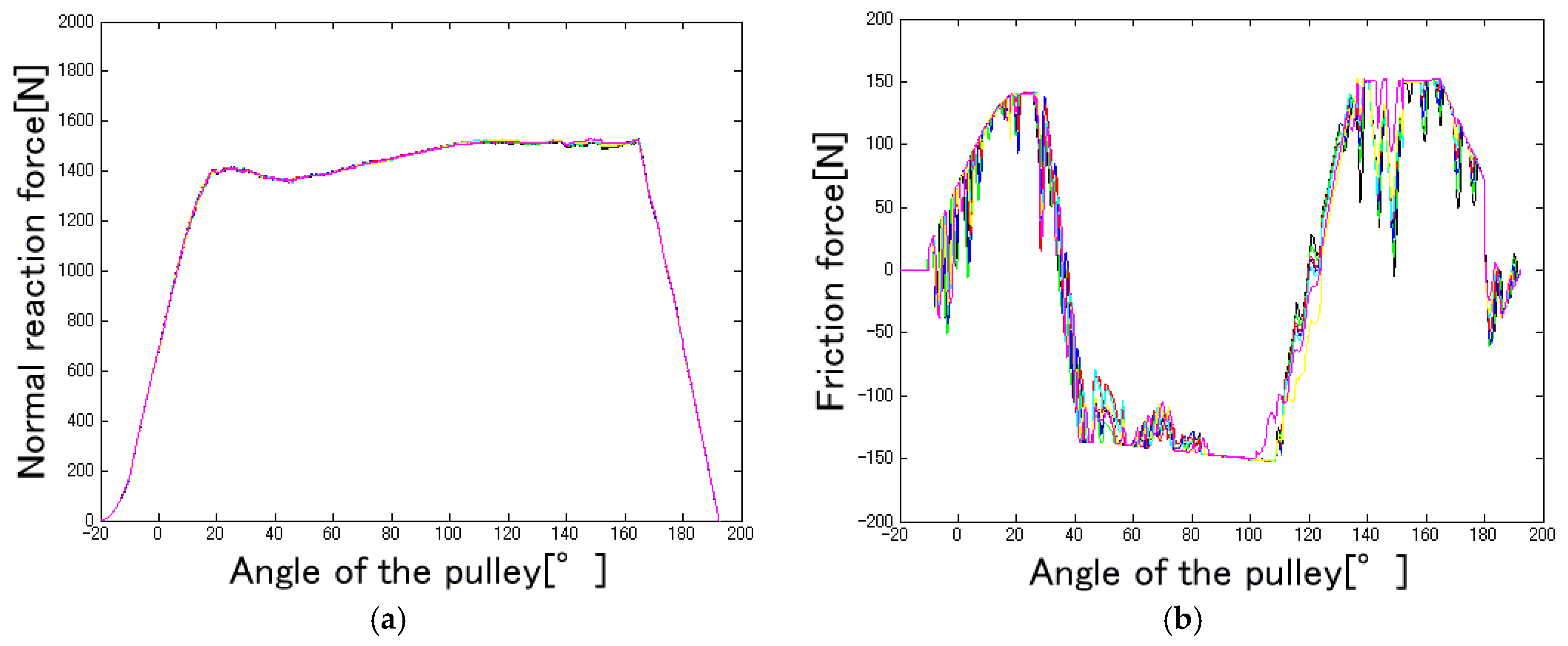
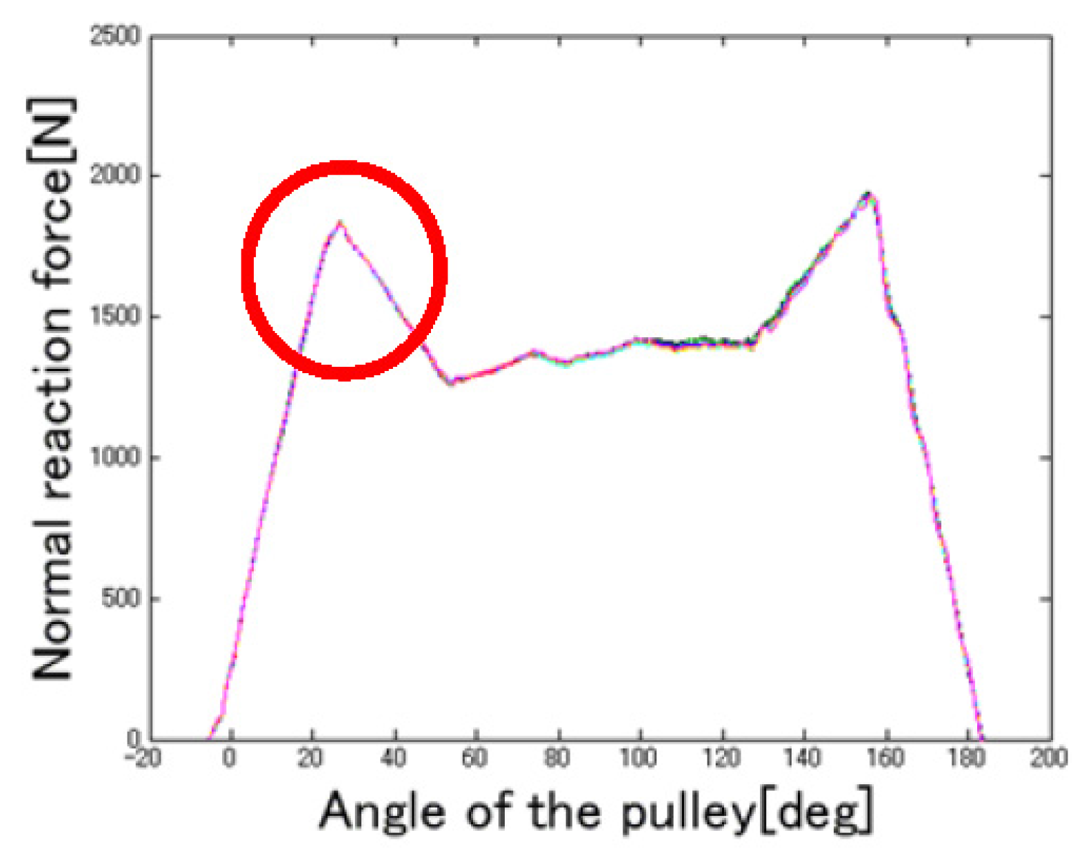
4.1. Force Acting on Rope

We consider the force that rotates the pulley and acts on the wire rope. Here, we will assume that a wire rope is wrapped around the stationary puller, and it then begins to rotate in the clockwise direction. The circumferential velocity of the pulley is 0.10 m/s. A normal contact force and a frictional force act on the 15th to 21st elements, as shown in Figure 8; Figure 9 shows the normal contact and frictional forces acting on each of the nodes. The colors of the nodal coordinates in Figure 8 correspond to the colors of the lines in Figure 9. In the initial condition, there is no contact between the wire rope and the pulley; contact occurs when the pulley begins to rotate. In Figure 9, the horizontal axis shows the clockwise rotational displacement of the pulley: The far left end represents 0°. The magnitude of the normal contact force, shown in Figure 9a, differs when the rotational angle of the pulley changes; although this force is symmetric when the pulley is at rest, it is changed by the rotation of the pulley. In this figure, we see that the contact force occurs for angles less than 0° and over 180° due to the transverse wave caused by the inertial force of the rope itself. We also note that the sign of the frictional force changes, as shown in Figure 9b. From these results, we see that the frictional force does not act uniformly on a rotating pulley. It was found that the rope was moved by the sum of these frictional forces. In this figure, the frictional force in the positive direction is the force that moves the rope in the rotational direction, and the frictional force in the negative direction is the force that moves the rope in the inverse rotational direction. Thus, it was shown that, when the difference between the right and left inertial forces was greater than the masses of the frictional forces in the direction opposite to that of the inertial force, the rope slides and the pulley is not able to move the rope.
Figure 8. Shape of a wire rope at start time.
Machines 04 00004 g008
Figure 9. Normal contact and frictional force at each node of the element. (a) Normal contact force; (b) frictional force.
Machines 04 00004 g009

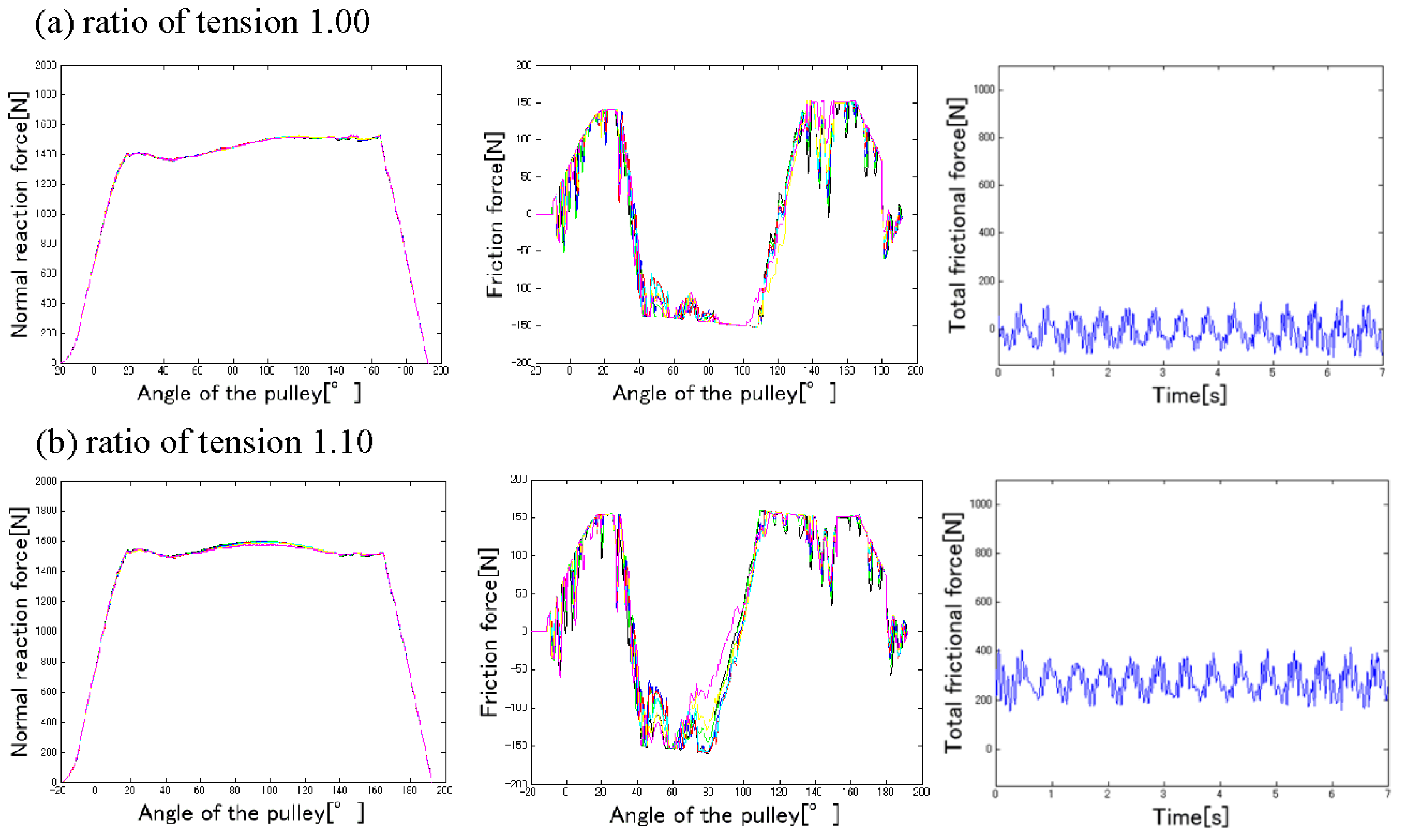
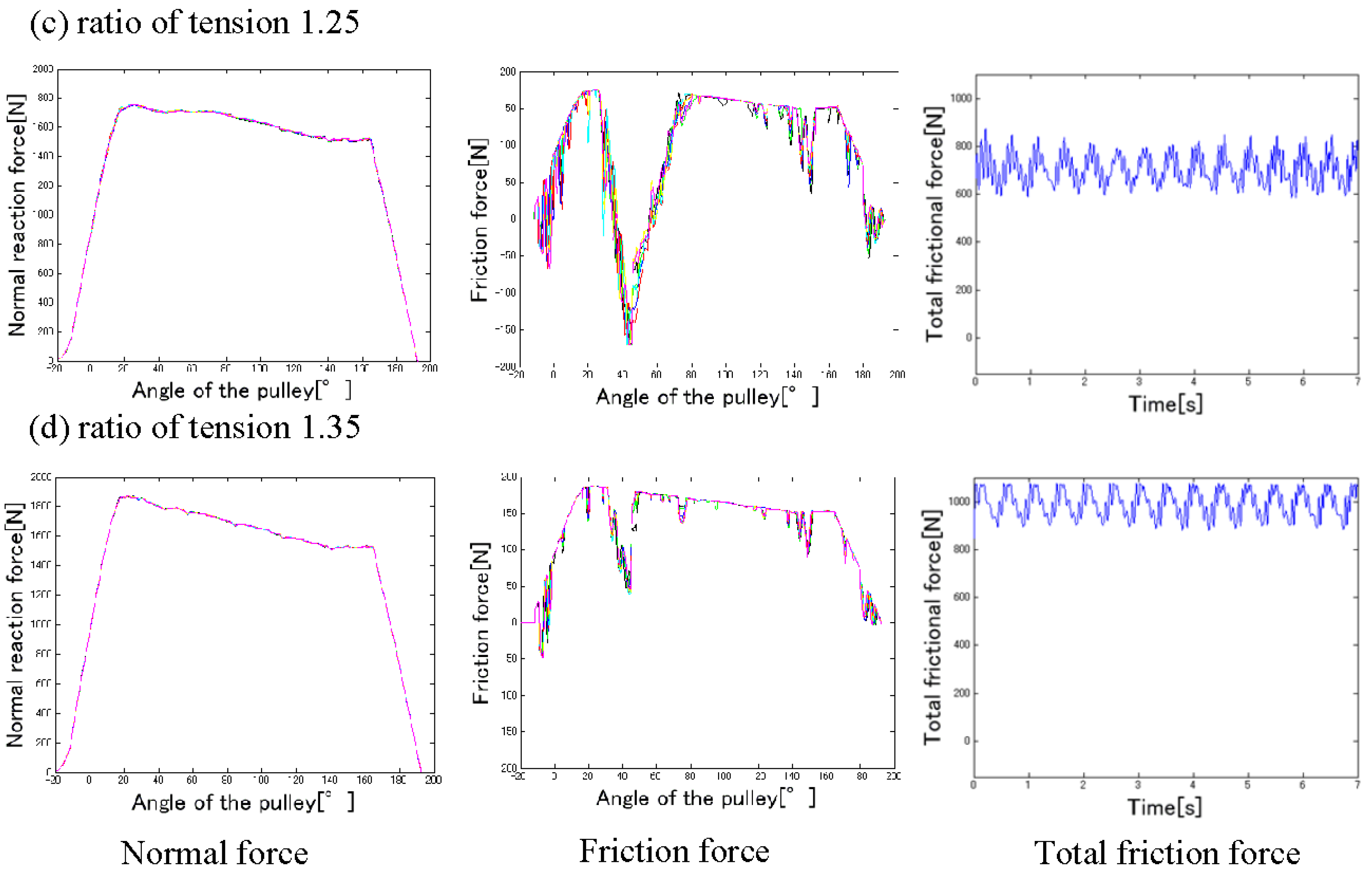
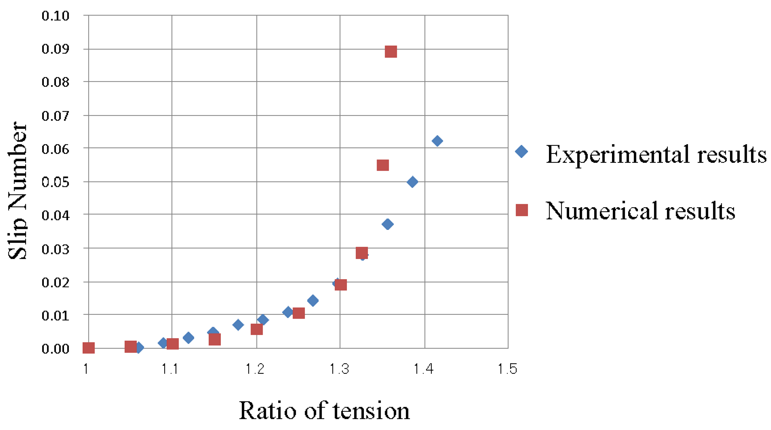
4.2. Influence of Ratio of Tension

In this section, we investigate the influence of the ratio of tension, which is the ratio of the weights applied to each end of the rope. The weight added on the right end of the rope was 294.70 kg, and we performed numerical simulations in which different weights were added on the left side. Figure 10 shows the normal contact force and the friction acting on each nodal coordinate when the ratio of tension varied from 1.00 to 1.35. First, we consider the normal contact force. When the mass on the left side is greater, the force that acts on the left side of the pulley is larger. The load on the pulley does not increase uniformly when the ratio of tension is large. Next, we consider the frictional force. Figure 10 shows the magnitude and area of the counterclockwise frictional force when the ratio of tension is 1.00; note that, as the rotational angle changes from 40° to 110°, the force becomes smaller. The reason why the frictional force in the negative direction always occurs at 40° is that the weight on the left side does not change. This angle is decided by the radius of the pulley and the weight on the left. The time history of the sum of the frictional forces as the ratio of tension varies from 1.00 to 1.35 is shown in Figure 10, and we can see that the sum of the frictional forces acting on the rope increases when the ratio of tension increases. This is because the difference between the inertial forces of the masses on the right and left sides is equal to the frictional force. As an example, consider the case in which the ratio of tension is 1.35: We have 0.35 × 294.7 k g × 9.81 m / s 2 1012 N . In addition, in Figure 10, we can see that the sum of the frictional forces oscillates as the nodal coordinate makes and breaks contact with the pulley. The contact velocity of each nodal coordinate when the ratio of tension varies from 1.00 to 1.35 is shown in Figure 10. Here, the contact velocity is taken to be v ¯ in Equation (13), and its value can be used to define whether slip has occurred. From Equation (13), we can determine that the nodal coordinate has slipped and that there is a kinetic frictional force when | v ¯ | > ε . Figure 10 shows that the nodal coordinate slips at some angles, but not at others; we can see that the range of slip increases when the ratio of tension increases. From Equation (13), we see that the maximum of the frictional force is μ N . When all the frictional forces on the pulley are at a maximum, the wire rope slips, and the pulley cannot move it.
Figure 10. Time history of each force for ratios of tension between 1.00 and 1.35.
Machines 04 00004 g010aMachines 04 00004 g010b

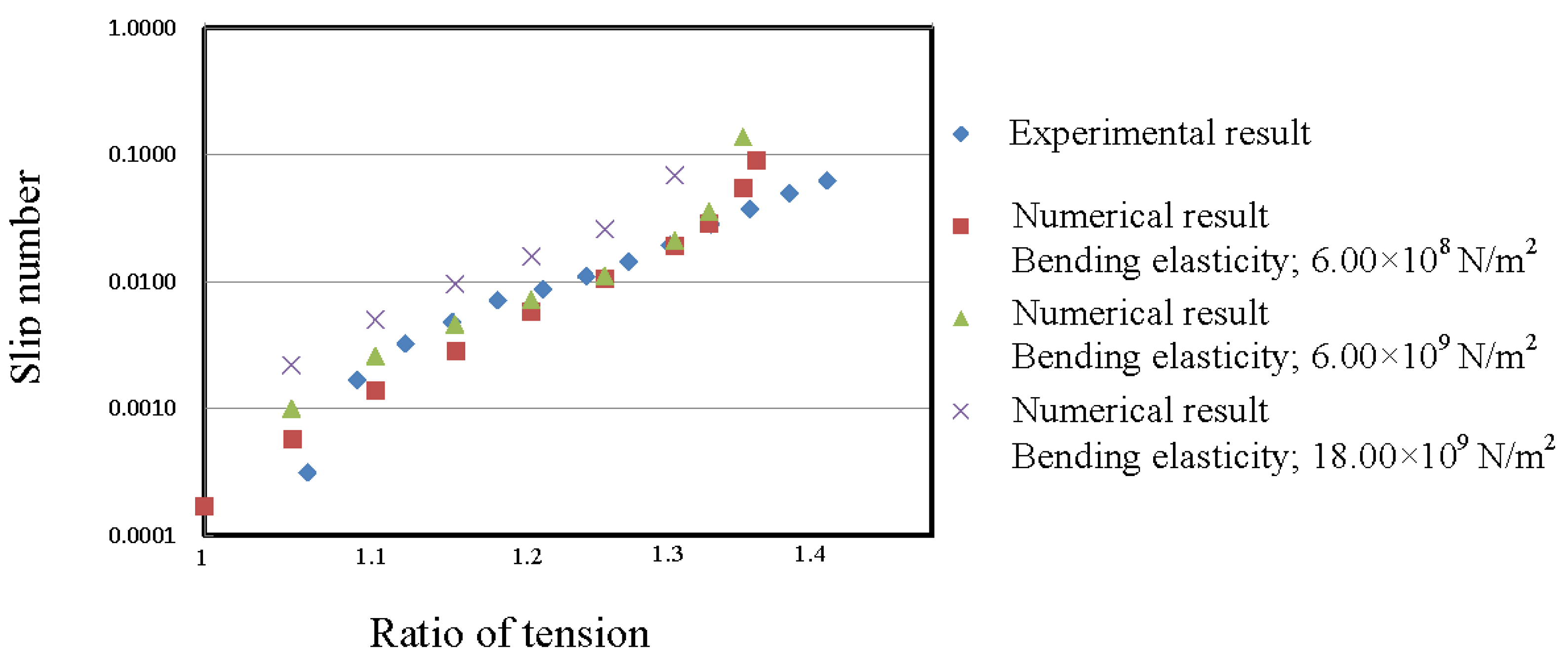
4.3. Influence of Bending Elastic Modulus

We investigated the slip when the bending elastic modulus of the rope was changed, and the pulley had reciprocal motion. Figure 11 shows the slip numbers for the experiment and the numerical simulations when the bending elastic modulus was changed as follows: 6.00 × 10⁸ N/m2, 6.00 × 10⁹ N/m2, and 18.00 × 10⁹ N/m2. The other parameters are the same as those listed in Table 2. In Figure 11, results of three numerical simulations are compared, and it can be seen that the slip number increases when the ratio of tension is low and that the bending elastic modulus is high. The reason for this is that the contact force between the rope and the pulley is smaller, since it is hard for the rope to bend when the bending elastic modulus is large. Figure 12 shows the normal contact force acting on each nodal coordinate when the bending elastic modulus is 6.00 × 10⁹ N/m2. In Figure 12, it is found that there is a characteristic area, indicated by a red circle. The wire rope contacts only the edges of the pulley, because the bending elastic modulus is high. The normal contact force is larger in this area because the area of contact is small. Therefore, slip occurs easily because the total frictional force is small.
Figure 11. Ratio of tension vs. slip number for various values of the bending elasticity.
Machines 04 00004 g011
Figure 12. Normal contact force at each node of the element.
Machines 04 00004 g012

5. Conclusions

In this paper, we developed a numerical model that can be used for detailed analyses of the behavior of the contact between a wire rope and a pulley; the model uses multibody dynamics. Our proposal and findings are summarized as follows.
  • We proposed a numerical model that can describe in detail the behavior of the contact between a wire rope and a pulley.
  • The validity of the developed numerical model was confirmed by comparing the distance of slip predicted by numerical simulations to that measured in experiments, when the wire rope had reciprocal motion.
  • From the results of the numerical simulations, we showed that the force acting on a wire rope on a pulley is not uniform, due to the action of partial forces.
  • From the results of the numerical simulations, it was determined that the rope slips when the ratio of tension is low, and the bending elastic modulus of the rope is large.

Acknowledgments

Sophia University and Tokyo Metropolitan University financially supported this research, and these contributions are highly appreciated.

Author Contributions

Shoichiro Takehara and Masaya Kawarada formulated the numerical model; Masaya Kawarada coded the numerical model and performed the experiments; Shoichiro Takehara, Masaya Kawarada and Kazunori Hase analyzed the data and discussed the results; Shoichiro Takehara wrote the paper.

Conflicts of Interest

The authors declare no conflict of interest.

References

  1. Terumichi, Y.; Yoshizawa, M.; Fukawa, Y.; Tsujioka, Y. Lateral oscillation of a moving elevator rope a cab in high-rise building. Trans. Jpn. Soc. Mech. Eng. 1993, 59, 686–693. [Google Scholar] [CrossRef]
  2. Nohmi, M.; Yoshida, S.; Terumichi, Y.; Takehara, S.; Uchiyama, M.; Nencherv, D. Space environmental test for a tethered space robot. Space Utiliz. Res. 2008, 24, 115–116. [Google Scholar]
  3. Nohmi, M.; Yoshida, S. Experimental analysis for attitude control of a tethered space robot under microgravity. Space Technol. 2004, 24, 119–128. [Google Scholar]
  4. Kimura, H.; Min, Z.; Ishii, T.; Yamamoto, A.; Shiba, H. Vibration analysis of elevator rope(simplified calculation method for detecting rope deflection of moving cage during earthquake). Trans. Jpn. Soc. Mech. Eng. 2009, 75, 2483–2488. [Google Scholar] [CrossRef]
  5. Kaczmarczyk, S.; Ostachowicz, W. Non-stationary responses of cables with slowly varying length. J. Acoust. Vib. 2000, 5, 117–126. [Google Scholar]
  6. Imanishi, E.; Nanjo, T.; Hirooka, E.; Kobayashi, T. Dynamic simulation of a wire rope with contact. Trans. Jpn. Soc. Mech. Eng. 2004, 70, 1023–1028. [Google Scholar] [CrossRef]
  7. Klaus, F. Wire Ropes; Springer: Berlin, Germany, 2007; pp. 194–195. [Google Scholar]
  8. Shabana, A.A. Finite element incremental approach and exact rigid body inertia. J. Mech. Des. 1996, 118, 171–178. [Google Scholar] [CrossRef]
  9. Shabana, A.A.; Hussien, H.A.; Escalona, J.L. Application of the absolute nodal coordinate formulation to large rotation and large deformation problems. J. Mech. Des. 1998, 120, 188–195. [Google Scholar] [CrossRef]
  10. Takahashi, Y.; Shimizu, N.; Suzuki, K. Study on the damping matrix of the beam element formulated by absolute nodal coordinate approach. Trans. Jpn. Soc. Mech. Eng. 2003, 69, 2225–2232. [Google Scholar] [CrossRef]
  11. Takahashi, Y.; Shimizu, N. Study on the elastic force for the deformed beam by means of the absolute nodal coordinate multibody dynamics formulation (Derivation of the elastic force using finite displacement and infinitesimal strain). Trans. Jpn. Soc. Mech. Eng. 2001, 67, 626–632. [Google Scholar] [CrossRef]
  12. Abdullah, A.M.; Michitsuji, Y.; Takehara, S.; Nagai, M.; Miyajima, N. Swing-up control of mass body interlinked flexible tether. Arch. Mech. Eng. 2010, 57, 115–131. [Google Scholar] [CrossRef]
  13. Quinn, D.D. A new regularization of coulomb friction. J. Vib. Acoust. 2004, 126, 391–397. [Google Scholar] [CrossRef]
  14. Karnopp, D. Computer simulation of stick-slip friction in mechanical dynamic systems. J. Dyn. Syst. Meas. Control 1985, 107, 100–103. [Google Scholar] [CrossRef]
  15. Salcudean, E.S.; Vlaar, T. On the emulation of stiff walls and static friction with a magnetically levitated input-output device. J. Dyn. Syst. Meas. Control 1997, 119, 127–132. [Google Scholar] [CrossRef]
  16. Yagawa, G.; Hirayama, H.; Ando, Y. Analysis of two-dimensional bodies and beams in contact using penalty function method. Trans. Jpn. Soc. Mech. Eng. 1980, 46, 1220–1229. [Google Scholar] [CrossRef]
  17. ImageJ. Available online: http://rsbweb.nih.gov/ij/ (accessed on 19 January 2016).
  18. Laboratory of Plant Cell Biology in Totipotency Homepage. Available online: http://hasezawa.ib.k.u-tokyo.ac.jp/zp/Kbi/ImageJ/) (accessed on 19 January 2016).

