Motion Error Prediction of Linear Axis Considering Tolerance Coupling and Worktable Elastic Deformation

Abstract

The linear axis is a core motion module in precision equipment and directly affects assembly and machining accuracy. Inaccurate prediction of motion error may lead to failure in aerospace manufacturing and assembly. Most existing methods typically assume rigid components and neglect tolerance coupling, yielding inaccurate predictions. Therefore, a method considering both tolerance coupling and worktable elastic deformation is developed. First, the variation ranges of geometric errors under the coupled tolerances were characterized using Small Displacement Torsor theory. Second, a two-stage error propagation model is established: errors were initially propagated from the base to four sliders by Homogeneous Transformation Matrices, and subsequently mapped to the worktable utilizing transfer coefficients derived from finite element analysis. Finally, Monte Carlo Simulation was employed to obtain the error variation intervals and their statistical distributions. A case study demonstrated that neglecting worktable elastic deformation underestimates translational errors by up to 40%. Meanwhile, neglecting tolerance coupling would underestimate rotational and translational errors by up to 43% and 25%, respectively. Furthermore, applying the proposed model to tolerance allocation proved that the schemes guided by simplified models would cause critical design failures. Therefore, incorporating both factors is important for obtaining physically grounded error predictions and for improving the reliability of tolerance allocation.

1. Introduction

The linear axis is a core motion module in precision manufacturing equipment, including industrial automation systems, aerospace manufacturing and assembly systems, and ultra-precision machine tools [1]. Its typical structure consists of a stationary base with two guideways, four sliders that move along the guideways, and a worktable mounted on the sliders to carry the tool or workpiece. In the high-end applications, the spatial motion errors of the linear axis directly govern the terminal volumetric accuracy of the equipment, where even sub-micron positional shifts or micro-radian angular drifts can lead to critical assembly misalignments or structural failure [2,3,4]. Although motion errors arise from multiple sources including thermal effects, dynamic vibrations, and servo control deviations [5,6,7,8], geometric errors associated with component manufacturing tolerances remain one of the dominant contributors [9]. In current industrial practice, designers typically attempt to ensure motion accuracy either by tightening individual component tolerances or by relying on post-assembly error compensation. However, the former exponentially increases manufacturing costs and quickly reaches physical machining limits, while the latter is constrained by measurement accessibility and dynamic operating conditions. Therefore, establishing a reliable error prediction model at the preliminary design stage is of paramount significance. Such proactive prediction enables designers to establish the mapping between component tolerances and linear axis motion errors, thereby providing a basis for tolerance allocation and enabling a more predictive approach to precision design. To establish a reliable error prediction model, considerable research has been conducted on tolerance modeling, tolerance analysis, error propagation and error prediction.

Tolerance modeling is the foundation of tolerance analysis. Commonly used tolerance modeling methods include the Small Displacement Torsor (SDT), Skin Model, Vector-Loop model, T-Map, among others. The choice of tolerance analysis method depends on the specific tolerance model, with prevalent approaches including the worst-case method, statistical method, and Monte Carlo Simulation (MCS) [10,11,12,13]. Guo et al. [14] developed a tolerance model for the linear axis based on SDT and expressed the torsor parameters as periodic functions of tolerances. Li et al. [15] utilized SDT to represent the tolerances of the linear motion axis and incorporated them into MCS. Zhou et al. [16] proposed a deviation propagation and small displacement torsor method for analyzing component tolerances and their propagation during assembly. Wu et al. [17] established constraint relationships between SDT parameters and tolerance, and constructed a mapping model of SDT parameters to error variation intervals via MCS. Fan et al. [18] employed truncated Fourier series to represent guideway errors while constraining the function variations within tolerance limits. However, these studies typically assume that each geometric tolerance acts independently, neglecting the coupling effects between different tolerance types. For instance, the coupled influence of flatness and parallelism on the base can significantly change the error variation intervals of the linear axis.

Error propagation focuses on the accumulation laws of component errors after assembly. Current modeling approaches include Multi-Body System (MBS) [19], Homogeneous Transformation Matrix (HTM) [20], Screw Theory [21], and Jacobian–Torsor [22], among others. With error propagation models, engineers can predict final assembly errors and devise corresponding control strategies to ensure product quality. Fan et al. [23] established an error propagation model for the machine tool linear axis based on MBS and HTM. Du et al. [24] developed a linear axis error propagation model using the Jacobian–Torsor approach. Hui et al. [25] proposed a data-driven error prediction model for linear motion systems, which relies on extensive measurement data to improve accuracy. Wang et al. [26] established an error propagation model for the machine tool linear axis using Screw Theory, and constructed a mapping model from four-slider errors to worktable errors. However, the vast majority of error propagation models adopt the rigid-body assumption and determine worktable errors from the four-slider errors using simple arithmetic operations such as averaging and differencing. In high-precision applications, even small elastic deformation can amplify or redistribute the motion errors in ways that rigid-body models cannot capture, leading to inaccurate error prediction.

Therefore, increasing attention has been paid to error prediction models that account for elastic deformation effects. Guo et al. [27] developed a guideway assembly error model considering elastic interaction effects. Rahmani and Bleicher [28] studied the pattern of guideway error propagation to the worktable through experiments and finite element analysis. Tong et al. [29] proposed a 5-DOF static equilibrium model incorporating local elastic contacts, accurately resolving the propagation mechanism of guideway errors. Yan et al. [30] proposed a linear axis error prediction model that considers both manufacturing errors and assembly deformations. Guo et al. [31] investigated the influence of guideway geometric error shapes on linear axis errors. Dai et al. [32] established a mapping model between tolerances and linear axis errors via finite element analysis based on the small deformation assumption and superposition principle. Xu et al. [33] developed a propagation model from guideway raceway surface errors to linear axis errors through static analysis of the linear guide system. Wang et al. [34] proposed a straightness error prediction method that comprehensively considers guideway machining errors and bed mounting surface errors, which can be used to optimize the tightening strategy of guideway bolt groups. Niu et al. [35] proposed an error prediction method for the linear axis under uncertainty in thread friction coefficients. Sun et al. [36] established a finite element model including guideways, sliders, and the worktable, and investigated the error averaging effect under different guideway error conditions. Although these studies incorporate elastic deformation into error modeling, many FEA-based approaches for slider-to-worktable error propagation consider only the translational errors of the sliders. The rotational errors of the four sliders are often neglected, which may result in an incomplete description of worktable motion errors.

To overcome the above limitations, this paper proposes a linear axis error prediction method that simultaneously accounts for tolerance coupling and worktable elastic deformation. First, SDT is used to describe the error variations of geometric features, and the SDT variation ranges of the base under coupled parallelism and flatness tolerances, as well as the guideway straightness constraints, are derived. Second, HTM is employed to establish the error propagation model from the base to the four sliders, and finite element analysis (FEA) is adopted to obtain the error propagation law from the four sliders to the worktable. Finally, Monte Carlo simulation is performed to predict statistical variation of linear axis motion errors, and the results are compared with those of simplified methods. Through this comparison, the prediction resulting from the neglect of worktable elastic deformation and tolerance coupling is quantitatively evaluated. Subsequently, the proposed model is applied to a tolerance allocation case to examine the consequences of using simplified error models for tolerance design.

2. Coupled Tolerance Modeling of Linear Axis

2.1. Structure and Key Component Design Tolerances of Linear Axis

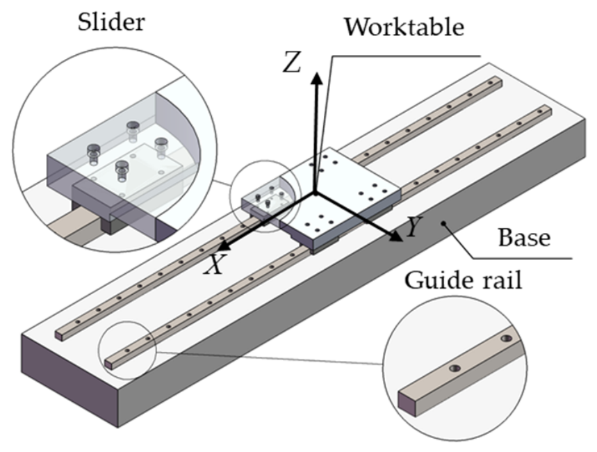
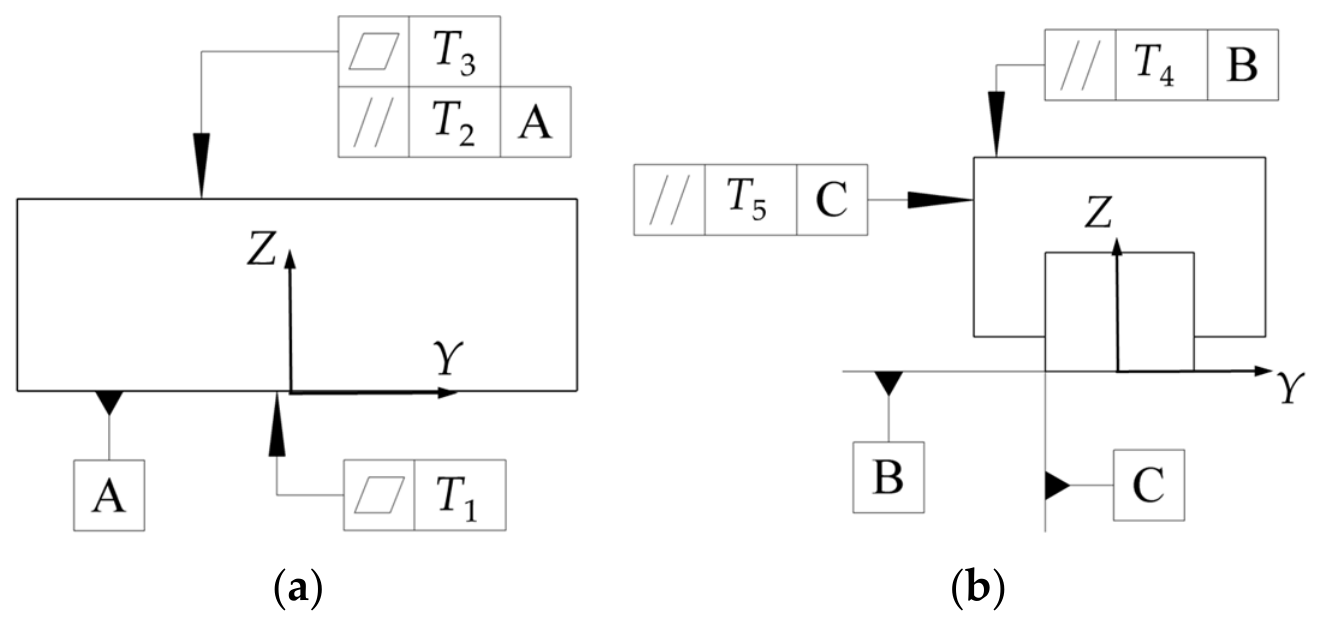
The typical structure of a linear axis is shown in Figure 1, which mainly consists of a base, two guide rails, four sliders, and a worktable. The key component design tolerances that affect its motion errors are illustrated in Figure 2. Here, T₁ and T₃ are the flatness tolerances of the upper and lower surfaces of the base, and T₂ is the parallelism tolerance between the upper and lower surfaces of the base, while T₄ and T₅ are the parallelism tolerances of the guideway–slider system in the Z-direction and Y-direction, respectively.

2.2. Description of Geometric Feature Error Variations Based on Small Displacement Torsor

The Small Displacement Torsor (SDT) is a mathematical tool based on rigid-body kinematics, used to describe the pose changes in a rigid body under small displacements. According to the Geometrical Product Specifications (GPS), the surfaces of a component can be abstracted as basic geometric features such as points, lines, and planes, and the small deviations of these geometric features from their nominal positions can be described by SDT [37,38]. An SDT can be expressed as (α, β, γ, u, v, w), where the six torsor parameters represent the small rigid-body deviations of a geometric feature relative to its nominal position in six degrees of freedom: α, β and γ denote the small rotations about the X, Y and Z axes, respectively, while u, v and w denote the small translations along the X, Y, and Z axes, respectively.

Consequently, the error variation of a geometric feature can be uniformly described by (α, β, γ, u, v, w). When a geometric feature translates along or rotates about a coordinate axis without changing its swept trajectory relative to its own geometric characteristics, the corresponding torsor parameter is set to zero. The design tolerances T₁–T₅ of the linear axis respectively constrain the error variation ranges of the geometric features to which they are applied. Among them, T₁ and T₃ are flatness tolerances, T₂ is a parallelism tolerance, and T₄ and T₅ are parallelism tolerances. Since the travel stroke of the guideway–slider system is typically much larger than its cross-sectional dimensions, T₄ and T₅ can be regarded as straightness acting on linear features. The tolerance zones of the three types of tolerances and their corresponding SDT descriptions are listed in

Table 1. SDT descriptions of linear axis tolerances.

Tolerances	Tolerance Zones	SDT
Y straightness (T5)		(0, β, γ, 0, v, w)
Z straightness (T4)
Flatness (T1, T3)		(α, β, 0, 0, 0, w)
Parallelism (T2)		(α, β, 0, 0, 0, w)

. Specifically, the error variation of the base surface can be described as (α, β, 0, 0, 0, w), and the error variation of the guideway–slider travel line can be described as (0, β, γ, 0, v, w).

2.3. Error Variation of the Base Surface Under Coupled Tolerances

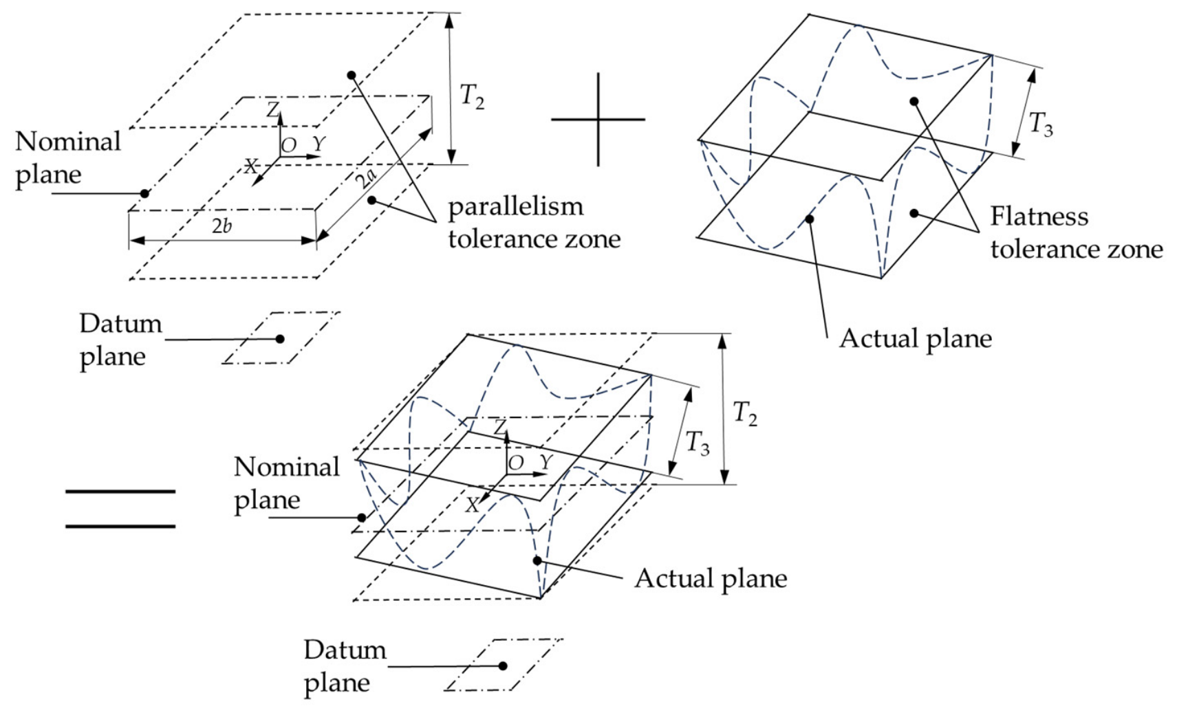
The tolerance zones of different tolerances impose constraints on the variation ranges of SDT. When multiple tolerances are applied simultaneously to the same geometric feature, the SDT variations become more complicated [39,40]. A typical case of multi-tolerance coupling occurs when the parallelism tolerance T₂ between the upper and lower surfaces of the base and the flatness tolerance T₃ of the upper surface are both specified on the same surface. It is therefore necessary to investigate the SDT variation range of a planar feature when multiple tolerances are assigned to it. In this paper, all tolerances are assumed to follow the independent principle. The tolerance modeling of the base planar feature under the coupling of parallelism and flatness is carried out based on SDT as follows.

A coordinate system is established with the center of the nominal plane as the origin and the Z-axis aligned with the normal direction of the nominal plane, as shown in Figure 3.

Under the coupling constraint of T₂ and T₃, the actual plane can only vary within the tolerance zone. Assume that the error variation of the actual plane is described by the SDT (α, β, 0, 0, 0, w), where α is the rotational deviation about the X-axis, β is the rotary deviation about the Y-axis, and w is the translational deviation along the Z-axis. The equation of this actual plane can be written as:

$$z=\alpha y-\beta x+w$$

(1)

The intersection line of the actual plane with the XOZ plane is:

$$z=-\beta x+w$$

(2)

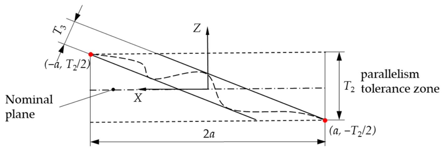
Assuming that the error variation of the actual plane is at its extreme, its projection on the XOZ plane is shown in Figure 4.

Let the nominal plane have a length of 2a and a width of 2b. When the actual plane is at its extreme error, the coordinates of the intersection points of the flatness tolerance zone with the upper and lower boundaries of the parallelism tolerance zone in the XOZ plane are (−a, T₂/2) and (a, −T₂/2), respectively. Substituting these points into Equation (2) yields the intersection lines of the upper and lower boundary planes of the flatness tolerance zone with the XOZ plane. Since these two lines are parallel and separated by a distance of T₃, we obtain:

$$-T_2/2=-{\beta }_{\max }\cdot a+w$$

(3)

$$T_2/2+T_3/\cos {\beta }_{\max }={\beta }_{\max }\cdot a+w$$

(4)

where β_max is the maximum rotation angle of the actual plane about the Y-axis under the coupled parallelism and flatness tolerances. Subtracting Equation (3) from Equation (4) gives:

$$T_2+T_3/\cos {\beta }_{\max }=2{\beta }_{\max }\cdot a$$

(5)

Since β is a small rotation angle, it can be approximated that cos β ≈ 1. Substituting this into the above yields:

$${\beta }_{\max }=(T_2+T_3)/2a$$

(6)

Similarly, we obtain:

$${\alpha }_{\max }=(T_2+T_3)/2b$$

(7)

Therefore, the SDT rotation parameters of the actual plane should not exceed the above maximum angles, and the error variation ranges under coupling are:

$$-(T_2+T_3)/2a\le \alpha \le (T_2+T_3)/2a$$

(8)

$$-(T_2+T_3)/2b\le \beta \le (T_2+T_3)/2b$$

(9)

While for the SDT translation parameter, it should not exceed the constraint imposed by the parallelism tolerance:

$$-T_2/2\le w\le T_2/2$$

(10)

Additionally, for any point (x, y) on the actual plane, the combination of the three torsor parameters must satisfy the following constraint:

$$-T_2/2\le \beta \cdot x+\alpha \cdot y+w\le T_2/2$$

(11)

Equations (8)–(11) constitute the SDT variation range of the base under the coupled constraints of parallelism and flatness. Compared with the case where only the flatness tolerance T₃ is considered, the coupled constraints of parallelism and flatness enlarge the SDT variation ranges of the upper base surface.

2.4. Error Variation of the Guideway–Slider System

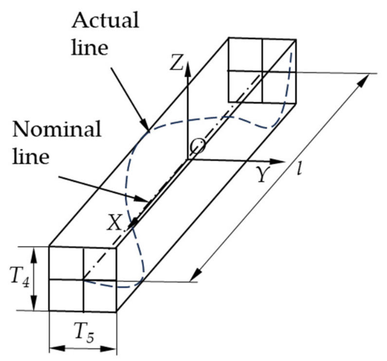
Since the stroke of the guideway–slider system is much larger than its cross-sectional dimensions, the parallelism tolerances T₄ and T₅ can be treated as straightness tolerances for the purpose of tolerance modeling.

As shown in Figure 5, the straightness errors in the Z- and Y-directions can be comprehensively described by the SDT (0, β, γ, 0, v, w), and the error variation ranges are given as follows:

$$-T_4/2\le w\le T_4/2$$

(12)

$$-T_4/l\le \beta \le T_4/l$$

(13)

$$-T_5/2\le v\le T_5/2$$

(14)

$$-T_5/l\le \gamma \le T_5/l$$

(15)

where l is the stroke of the guideway–slider system. The constraint conditions are:

$$-T_4/2\le w+\beta \cdot x\le T_4/2$$

(16)

$$-T_5/2\le v+\gamma \cdot x\le T_5/2$$

(17)

where x is any point along the stroke of the guideway–slider system. Equations (12)–(17) constitute the SDT variation ranges of the guideway–slider system under the constraints of the parallelism tolerances.

Unlike the base surface where flatness and parallelism tolerances are coupled, the parallelisms T₄ and T₅ constrain different degrees of freedom (Z- and Y-directions, respectively) of the guideway–slider system, thereby acting independently. Consequently, the coupled tolerance model of the base Equations (8)–(11) and the uncoupled tolerance model of the guideway–slider system Equations (12)–(17) collectively establish the geometric error variation ranges of the linear axis components. These SDT variation ranges serve as the inputs for the subsequent two-stage error propagation modeling and Monte Carlo Simulation.

3. Two-Stage Error Propagation Model

3.1. Overall Framework of Error Propagation for the Linear Axis

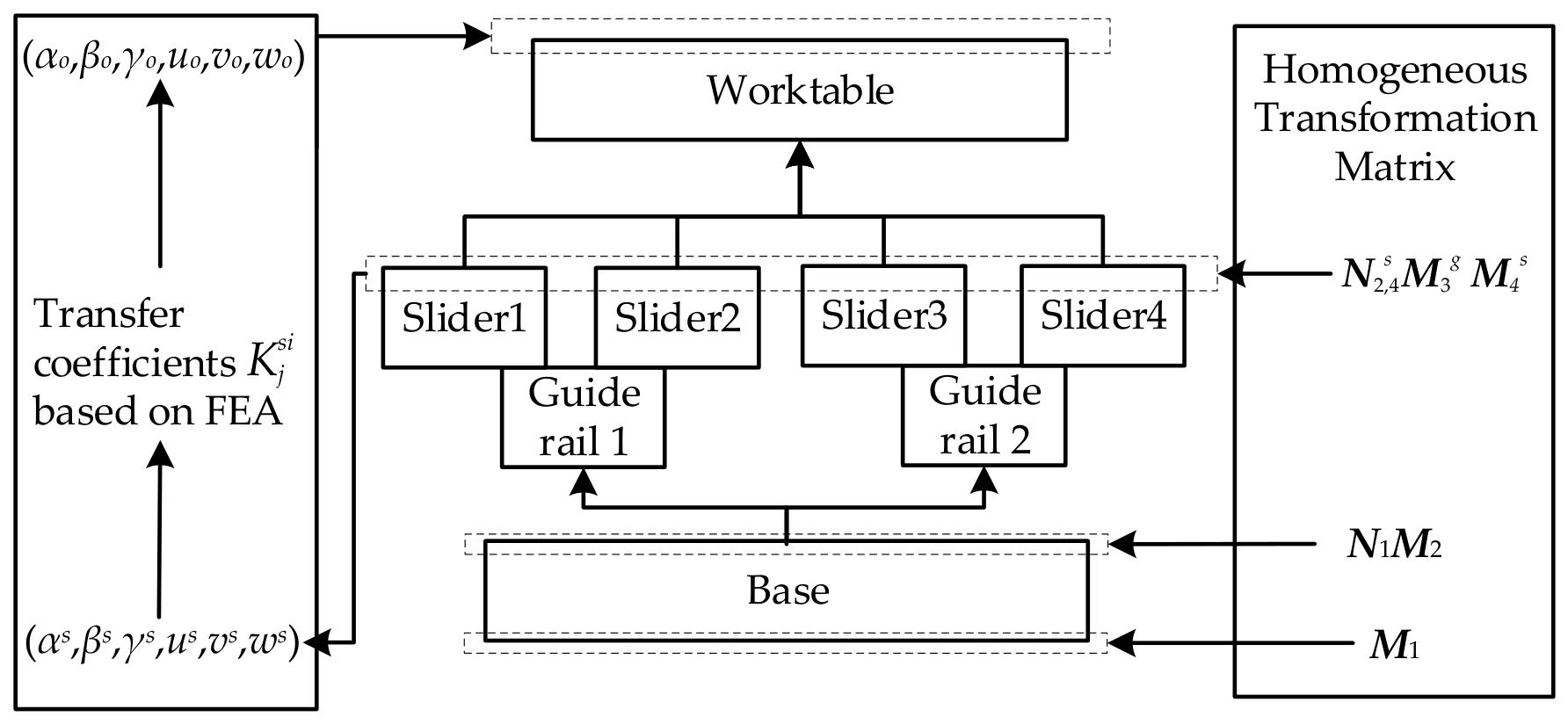
The output motion error of the linear axis is represented by the SDT parameters of the upper surface of the worktable, denoted as (α_o, β_o, γ_o, u_o, v_o, w_o), and a mapping model between the output errors and the errors of the individual components can be established. For a linear axis with two guide rails and four sliders configuration, the assembly relationship is illustrated in Figure 6. A two-stage error propagation model is constructed. In the first stage, the error propagation from the base to the four sliders follows a series relationship before the sliders are connected to the worktable, i.e., the errors are propagated sequentially along the path of “base → guide rail → slider.” Therefore, based on the HTM, four series error propagation chains from the base to the four sliders can be established. Then, in the second stage, the FEA is employed to analyze the error response of the worktable under the distinct translational errors and rotational errors of the four sliders, and a mapping model from the four-slider SDT (α^s, β^s, γ^s, u^s, v^s, w^s) to the worktable SDT is established.

3.2. Error Propagation Model from the Base to the Four Sliders

According to HTM, the actual pose transformation matrix for the final motion error output plane of slider s (s = 1, 2, 3, 4) on guideway g (g = 1, 2) with respect to the base datum plane can be expressed as:

$${\mathit{M}}^s={\mathit{M}}_1\times {\mathit{N}}_{1,2}\times {\mathit{M}}_2\times {\mathit{N}}_{2,4}^s\times {\mathit{M}}_3^g\times {\mathit{M}}_4^s(g=1,s=1,2;g=2,s=3,4)$$

(18)

Under ideal conditions without errors, the nominal pose transformation matrix is:

$${\mathit{N}}^s={\mathit{N}}_{1,2}\times {\mathit{N}}_{2,4}^s$$

(19)

where M₁, M₂, ${\mathit{M}}_3^g$, and ${\mathit{M}}_4^s$ denote the actual pose transformation matrix of the lower base surface, the upper base surface, the travel line of the guideway–slider system, and four sliders, respectively; N_1,2 denotes the nominal pose transformation matrix from the lower base surface to the upper base surface; and ${\mathit{N}}_{2,4}^s$ denotes the nominal pose transformation matrix from the upper base surface to the upper surface geometric center of slider s. These matrices are given explicitly as follows:

$$\left\{\begin{array}{lll}{\mathit{M}}_1=\left[\begin{array}{cccc}1& 0& {\beta }_1& 0\\ 0& 1& -{\alpha }_1& 0\\ -{\beta }_1& {\alpha }_1& 1& w_1\\ 0& 0& 0& 1\end{array}\right]& {\mathit{M}}_2=\left[\begin{array}{cccc}1& 0& {\beta }_2& 0\\ 0& 1& -{\alpha }_2& 0\\ -{\beta }_2& {\alpha }_2& 1& w_2\\ 0& 0& 0& 1\end{array}\right]& {\mathit{M}}_3^g=\left[\begin{array}{cccc}1& -{\gamma }_3^g& {\beta }_3^g& 0\\ {\gamma }_3^g& 1& 0& v_3^g\\ -{\beta }_3^g& 0& 1& w_3^g\\ 0& 0& 0& 1\end{array}\right]\\ {\mathit{M}}_4^1=\left[\begin{array}{cccc}1& 0& 0& 0\\ 0& 1& 0& \left|x_{2,4}^1\right|•{\gamma }_3^1\\ 0& 0& 1& -\left|x_{2,4}^1\right|•{\beta }_3^1\\ 0& 0& 0& 1\end{array}\right]& {\mathit{M}}_4^2=\left[\begin{array}{cccc}1& 0& 0& 0\\ 0& 1& 0& -\left|x_{2,4}^2\right|•{\gamma }_3^1\\ 0& 0& 1& \left|x_{2,4}^2\right|•{\beta }_3^1\\ 0& 0& 0& 1\end{array}\right]& {\mathit{M}}_4^3=\left[\begin{array}{cccc}1& 0& 0& 0\\ 0& 1& 0& \left|x_{2,4}^3\right|•{\gamma }_3^2\\ 0& 0& 1& -\left|x_{2,4}^3\right|•{\beta }_3^2\\ 0& 0& 0& 1\end{array}\right]\\ {\mathit{M}}_4^3=\left[\begin{array}{cccc}1& 0& 0& 0\\ 0& 1& 0& -\left|x_{2,4}^4\right|•{\gamma }_3^2\\ 0& 0& 1& \left|x_{2,4}^4\right|•{\beta }_3^2\\ 0& 0& 0& 1\end{array}\right]& {\mathit{N}}_{1,2}=\left[\begin{array}{cccc}1& 0& 0& x_{1,2}\\ 0& 1& 0& y_{1,2}\\ 0& 0& 1& z_{1,2}\\ 0& 0& 0& 1\end{array}\right]& {\mathit{N}}_{2,4}^s=\left[\begin{array}{cccc}1& 0& 0& x_{2,4}^s\\ 0& 1& 0& y_{2,4}^s\\ 0& 0& 1& z_{2,4}^s\\ 0& 0& 0& 1\end{array}\right]\end{array}\right.$$

(20)

Here, α₁, β₁, and w₁ are the SDT parameters constrained by the flatness tolerance T₁ of the lower base surface; α₂, β₂, and w₂ are the SDT parameters of the upper base surface under the coupled flatness tolerance T₃ and parallelism tolerance T₂; ${\beta }_3^g,{\gamma }_3^g,v_3^g,\mathrm{a}\mathrm{n}\mathrm{d} w_3^g$ (g = 1, 2) are the SDT parameters of the slider on guideway g under the constraints of the parallelism tolerance T₄ and T₅. x_1,2, y_1,2, and z_1,2 are the coordinate increments from the geometric center of the lower base surface to that of the upper base surface; $x_{2,4}^s, y_{2,4}^s, \mathrm{a}\mathrm{n}\mathrm{d} z_{2,4}^s$ (s = 1, 2, 3, 4) are the coordinate increments from the geometric center of the upper base surface to the geometric center of slider s. Consequently, the overall error transformation matrix from the base to slider s can be written as:

$${\mathit{E}}^s={\mathit{M}}^s-{\mathit{N}}^s+\mathit{I}=\left[\begin{array}{cccc}1& -{\gamma }^s& {\beta }^s& u^s\\ {\gamma }^s& 1& -{\alpha }^s& v^s\\ -{\beta }^s& {\alpha }^s& 1& w^s\\ 0& 0& 0& 1\end{array}\right]$$

(21)

where I is the 4 × 4 identity matrix. Equation (21) describes the error propagation relationship from the base to slider s, enabling mapping from the SDT of individual components to the SDT of each slider.

3.3. Error Propagation Model from the Four Sliders to the Worktable

To map the errors from the four sliders to the worktable, a simplified approach is to treat the worktable as a rigid body. Under this assumption, the SDT parameters of the worktable (α_o, β_o, γ_o, u_o, v_o, w_o) can be directly computed from the corresponding SDT parameters of the four sliders (α^s, β^s, γ^s, u^s, v^s, w^s) by geometric averaging and differencing as Equation (22):

$$\begin{array}{l}{u}_o={\displaystyle \frac{1}{4}}{\displaystyle {\displaystyle \sum _{s=1}^4}{u}^s}; v_o={\displaystyle \frac{1}{4}}{\displaystyle {\displaystyle \sum _{s=1}^4}{v}^s}; w_o={\displaystyle \frac{1}{4}}{\displaystyle {\displaystyle \sum _{s=1}^4}{w}^s}\\ {\alpha }_o={\displaystyle \frac{\frac{w^3+w^4}{2}-\frac{w^1+w^2}{2}}{D_y}}; {\beta }_o={\displaystyle \frac{\frac{w^2+w^4}{2}-\frac{w^1+w^3}{2}}{D_x}};\\ {\gamma }_o={\displaystyle \frac{1}{4}}\left({\displaystyle \frac{v^1-v^2}{D_x}}+{\displaystyle \frac{u^1-u^3}{D_y}}+{\displaystyle \frac{v^3-v^4}{D_x}}+{\displaystyle \frac{u^2-u^4}{D_y}}\right)\end{array}$$

(22)

where D_x and D_y are the installation distances between the sliders in the X- and Y-directions, respectively. Equation (22) is simple and computationally efficient, but it completely neglects the elastic deformation of the worktable and the interactions among the sliders. Consequently, it may lead to inaccurate error prediction.

Therefore, this section proposes a mapping method from the four-slider errors to the worktable errors based on the small deformation assumption and the superposition principle. The core idea of this method is to equivalently transform the errors of the four sliders into the interface surfaces between the sliders and the worktable, and then solve the response on the worktable errors through FEA.

3.3.1. Small Deformation Assumption and Superposition Principle

(1)

Small Deformation Assumption

The proposed mapping model is established under the small deformation assumption. When the deformation remains sufficiently small relative to the structural dimensions, the structural response can be approximated within the linear elastic regime. The assembly of the four sliders and the worktable constitutes a statically indeterminate system characterized by nonlinear contact interfaces. Under actual assembly conditions, the structural rigidity and the applied bolt preload define a stable localized equilibrium state. Because the slider errors (typically on the micrometer scale) act merely as micro-perturbations around this preloaded equilibrium, the stiffness of the contact interfaces remains approximately constant within this localized microscopic neighborhood. This approximately constant interfacial stiffness allows the nonlinear contact behavior to be locally linearized.

Assume that the Z-direction translational error parameter w^s of the slider s induces a Z-direction translational error parameter $w_o^{sw}$ of the worktable, denoted as $w_o^{sw}$ = f(w^s). Expanding this function by Taylor series at the zero-error state w^s = 0 yields:

$$w_o^{sw}=f(0)+f^{\prime }(0)w^s+{\displaystyle \frac{f^{″}(0)}{2!}}{(w^s)}^2+\cdots +{\displaystyle \frac{f^n(0)}{n!}}{(w^s)}^n$$

(23)

Since the errors of the four sliders are typically on the order of micrometers, which are far smaller than the structural dimensions of the linear axis, these errors constitute small deformations. Consequently, the error response of the worktable can be approximated as a linear relationship:

$$w_o^{sw}=f^{\prime }(0)w^s=K_w^{sw}{w}^s$$

(24)

where $K_w^{sw}$ denotes the transfer coefficient from the Z-direction translational error of slider s to the Z-direction translational error of the worktable. Similarly, the other error parameters α^s, β^s, γ^s, u^s and v^s of the slider s induce Z-direction translational error parameters $w_o^{s\alpha },w_o^{s\beta },w_o^{s\gamma },w_o^{su} \mathrm{a}\mathrm{n}\mathrm{d} w_o^{sv}$ of the worktable, which can be expressed as:

$$\left\{\begin{array}{l}{w}_o^{s\alpha }=K_w^{s\alpha }{\alpha }^s\\ w_o^{s\beta }=K_w^{s\beta }{\beta }^s\\ w_o^{s\gamma }=K_w^{s\gamma }{\gamma }^s\\ w_o^{su}=K_w^{su}{u}^s\\ w_o^{sv}=K_w^{sv}{v}^s\end{array}\right.$$

(25)

where $K_j^{si}$ denotes the transfer coefficient from the error parameter i (i = α, β, γ, u, v, w) of slider s to the worktable error parameter j (j = α, β, γ, u, v, w). From Equations (24) and (25), it can be seen that the small deformation assumption ensures a linear relationship between each worktable error parameter and the 24 error parameters of four sliders.

(2)

Superposition Principle

The superposition principle states that within the small deformation range, the effects of multiple independent loads or factors can be linearly superposed, i.e., the total response equals the vector sum of the responses produced by each factor acting individually.

For a linear axis with four sliders, according to the superposition principle, the worktable Z-direction translational error w_o under the combined contributions of all sliders can be expressed as the linear superposition of the contributions of each slider SDT (α^s, β^s, γ^s, u^s, v^s, w^s) acting individually:

$$w_o={\displaystyle {\displaystyle \sum _{s=1}^4}(w_o^{s\alpha }}+w_o^{s\beta }+w_o^{s\gamma }+w_o^{su}+w_o^{sv}+w_o^{sw})={\displaystyle {\displaystyle \sum _{s=1}^4}(K_w^{s\alpha }{\alpha }^s}+K_w^{s\beta }{\beta }^s+K_w^{s\gamma }{\gamma }^s+K_w^{su}{u}^s+K_w^{sv}{v}^s+K_w^{sw}{w}^s)$$

(26)

The adoption of the small deformation assumption and the superposition principle resolves the computational bottleneck associated with large-scale error prediction. The connection between the four sliders and the worktable constitutes a highly statically indeterminate and nonlinear system. In the Monte Carlo Simulation detailed in subsequent sections, a massive number of random samples need to be evaluated. Performing a complete FEA for each random sample is computationally infeasible.

However, this theoretical framework effectively decouples the complex nonlinear contact behavior into a linear combination of independent responses. Consequently, instead of executing a large number of FEA simulations, the system requires only a relatively small number to obtain transfer coefficients. Once these transfer coefficients are obtained, the subsequent massive number of sample evaluations can be executed instantaneously via linear combination.

It should be emphasized that the constancy of the transfer coefficients $K_j^{si}$ is physically bounded by the linear elastic range and stable interface states. The parameters rely on the nominal bolt preload and localized contact stiffness. Variations in bolt preload or extreme error perturbations beyond the micrometer regime could induce localized nonlinearities, which will be further discussed in the Section 5.6.

3.3.2. Mapping and Verification from Four Slider Errors to Worktable Errors

According to the small deformation assumption and the superposition principle, the remaining five SDT parameters of the worktable (α_o, β_o, γ_o, u_o, v_o) can be expressed in the same form as Equations (23)–(26):

$$\begin{array}{l}{\alpha }_o={\displaystyle \sum _{s=1}^4(K_{\alpha }^{s\alpha }{\alpha }^s}+K_{\alpha }^{s\beta }{\beta }^s+K_{\alpha }^{s\gamma }{\gamma }^s+K_{\alpha }^{su}{u}^s+K_{\alpha }^{sv}{v}^s+K_{\alpha }^{sw}{w}^s)\\ {\beta }_o={\displaystyle \sum _{s=1}^4(K_{\beta }^{s\alpha }{\alpha }^s}+K_{\beta }^{s\beta }{\beta }^s+K_{\beta }^{s\gamma }{\gamma }^s+K_{\beta }^{su}{u}^s+K_{\beta }^{sv}{v}^s+K_{\beta }^{sw}{w}^s)\\ {\gamma }_o={\displaystyle \sum _{s=1}^4(K_{\gamma }^{s\alpha }{\alpha }^s}+K_{\gamma }^{s\beta }{\beta }^s+K_{\gamma }^{s\gamma }{\gamma }^s+K_{\gamma }^{su}{u}^s+K_{\gamma }^{sv}{v}^s+K_{\gamma }^{sw}{w}^s)\\ u_o={\displaystyle \sum _{s=1}^4(K_u^{s\alpha }{\alpha }^s}+K_u^{s\beta }{\beta }^s+K_u^{s\gamma }{\gamma }^s+K_u^{su}{u}^s+K_u^{sv}{v}^s+K_u^{sw}{w}^s)\\ v_o={\displaystyle \sum _{s=1}^4(K_v^{s\alpha }{\alpha }^s}+K_v^{s\beta }{\beta }^s+K_v^{s\gamma }{\gamma }^s+K_v^{su}{u}^s+K_v^{sv}{v}^s+K_v^{sw}{w}^s)\end{array}$$

(27)

To verify the applicability of the small deformation assumption and the superposition principle, FEA was performed to examine the applicability of the mapping model within the prescribed SDT ranges. Under the small deformation assumption and the superposition principle, the variation ranges of the slider SDT were set as follows: (−6 × 10⁻⁵ ≤ α^s ≤ 6 × 10⁻⁵, −2 × 10⁻⁵ ≤ β^s ≤ 2 × 10⁻⁵, −2 × 10⁻⁵ ≤ γ^s ≤ 2 × 10⁻⁵, −3 ≤ u^s ≤ 3, −15 ≤ v^s ≤ 15, −30 ≤ w^s ≤ 30), where the rotational error parameters are in radians and the translational error parameters are in micrometers. Within these ranges, the worktable error responses were solved using FEA.

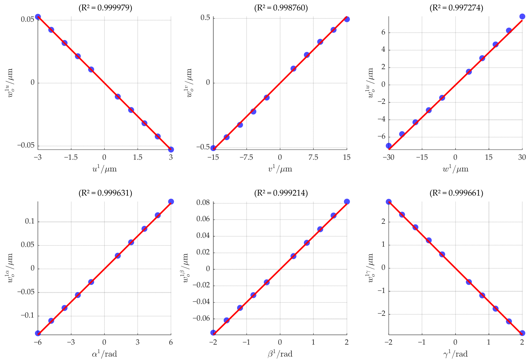
As shown in Figure 7, scatter plots of the relationship between slider errors and worktable errors were generated and fitted to linear curves. It can be observed that the SDT of Slider 1 (α¹, β¹, γ¹, u¹, v¹, w¹) and the resulting worktable error parameters $\left(w_o^{1\alpha }, w_o^{1\beta }, w_o^{1\gamma }, w_o^{1u}, w_o^{1v}, w_o^{1w}\right)$ exhibit a high degree of linear correlation. The coefficients of determination R² for all fitted curves are equal to 1. In addition, the linear correlations for the remaining sliders were also verified, with R² values all greater than 0.994. These results indicate that, within the given slider SDT variation ranges, the worktable SDT response caused by any individual SDT parameter of sliders follows a linear relationship, thus satisfying the small deformation assumption.

To verify the validity of the superposition principle, a comparative FEA test was designed. Multiple sets of values were randomly selected within the slider SDT variation ranges, and the results obtained under simultaneous variations of multiple slider SDT (Result 1) were compared with the linearly superposed results from individual slider SDT variations (Result 2). One of the comparisons is presented in

Table 2. Verification calculation results of the superposition principle.

Category	αo	βo	γo	uo	vo	wo
Result 1	1.049 × 10−4	2.831 × 10−3	7.750 × 10−3	−1.819 × 10−5	1.014 × 10−6	3.689 × 10−7
Result 2	1.021 × 10−4	2.729 × 10−3	7.703 × 10−3	−1.811 × 10−5	9.901 × 10−7	3.670 × 10−7
Relative error	2.638%	3.622%	0.604%	0.474%	2.313%	0.510%

. The relative errors remain below 3.7%, indicating good agreement between the simultaneous FEA results and the linearly superposed responses within the investigated range, thereby confirming the applicability of the superposition principle.

In summary, the FEA verification demonstrates that the error mapping model between the four slider errors and the worktable errors established using the small deformation assumption and the superposition principle is applicable. However, the validity of this model is limited to the specific SDT range.

3.3.3. Solution of Transfer Coefficients

This subsection presents a method for determining the transfer coefficients $K_j^{si}$ based on FEA. The method involves taking test points within the SDT variation ranges of the sliders, computing the deformation response of the linear axis at the output position on the upper surface of the worktable via FEA, and then fitting an error plane to obtain the SDT of the worktable. The specific steps are as follows:

Step 1: Change the error parameter i^s (i = α, β, γ, u, v, w) of slider s (s = 1, 2, 3, 4), and perform FEA to compute the worktable response under this single error condition.

Step 2: Extract a set of discrete points on the upper surface of the worktable, and fit an error plane using the least-squares method. The SDT deviation of this plane relative to the nominal plane, denoted as $\left({\alpha }_o^{si},{\beta }_o^{si},{\gamma }_o^{si},u_o^{si},v_o^{si},w_o^{si}\right)$, represents the worktable response induced by the single error parameter of the slider.

Step 3: Taking the slider error variation i^s as the independent variable and the worktable response (${\alpha }_o^{si}, {\beta }_o^{si},{\gamma }_o^{si},u_o^{si},v_o^{si},w_o^{si}$) as the dependent variables, apply the least-squares method to determine the transfer coefficients $K_j^{si}$ (j = α, β, γ, u, v, w).

Each slider error variation yields six transfer coefficients. With six error parameters for each of the four sliders, there are 24 error variation cases in total, resulting in all 6 × 24 = 144 transfer coefficients.

4. Motion Error Prediction Based on Monte Carlo Simulation

The Monte Carlo Simulation (MCS) is a numerical computational approach based on random sampling. Its fundamental principle is to estimate unknown quantities or their distributions through extensive random sampling, thereby obtaining approximate solutions via statistical calculations. In Section 2, the error variation ranges of the parameters of the linear axis were derived. Based on MCS, random error samples can be generated within these variation ranges and subsequently used as inputs to the error propagation model established in Section 3, from which the resulting worktable errors can be obtained.

4.1. SDT Generation of Linear Axis

Step 1: Determination of the distribution type of SDT.

In the forward design stage, empirical process data are typically unavailable prior to batch production. Following the Central Limit Theorem, component errors are conventionally modeled as normal distributions within the tolerance zones [41]. The sensitivity of the predictions to alternative error distributions is evaluated in Section 5.6.2. Accordingly, the generated SDT parameters are assumed to be normally distributed, with the probability density function $\phi \left(x\right)$ expressed as:

$$\phi \left(x\right)={\displaystyle \frac{1}{\sqrt{2\pi }\sigma }}{e}^{{\displaystyle \frac{{(x-\mu )}^2}{2{\sigma }^2}}}\hspace{1em}\hspace{1em}\hspace{1em}x=(\alpha ,\beta ,w)$$

(28)

where μ denotes the mean, and σ denotes the standard deviation. The effective range of a normal distribution is typically taken as ±3σ, which can be mapped to the boundaries of the error variation ranges. Therefore, for the base surface SDT (α, β, 0, 0, 0, w), based on their error variation ranges from Equations (8) to (10), the means are ${\mu }_{\alpha }={\mu }_{\beta }={\mu }_w=0$. Taking the boundaries of the error variation ranges as 3σ, the variances are ${\sigma }_{\alpha }^2=({(T_2+T_3)/6b)}^2$, ${\sigma }_{\beta }^2=({(T_2+T_3)/6a)}^2$, and ${\sigma }_w^2=({(T_2)/6)}^2$. Thus, they can be considered to follow normal distributions with the following parameters:

$$\left\{\begin{array}{c}\alpha ~N(0,{({\displaystyle \frac{T_2+T_3}{6b}})}^2)\\ \beta ~N(0,{({\displaystyle \frac{T_2+T_3}{6a}})}^2)\\ w~N(0,{({\displaystyle \frac{T_2}{6}})}^2)\end{array}\right.$$

(29)

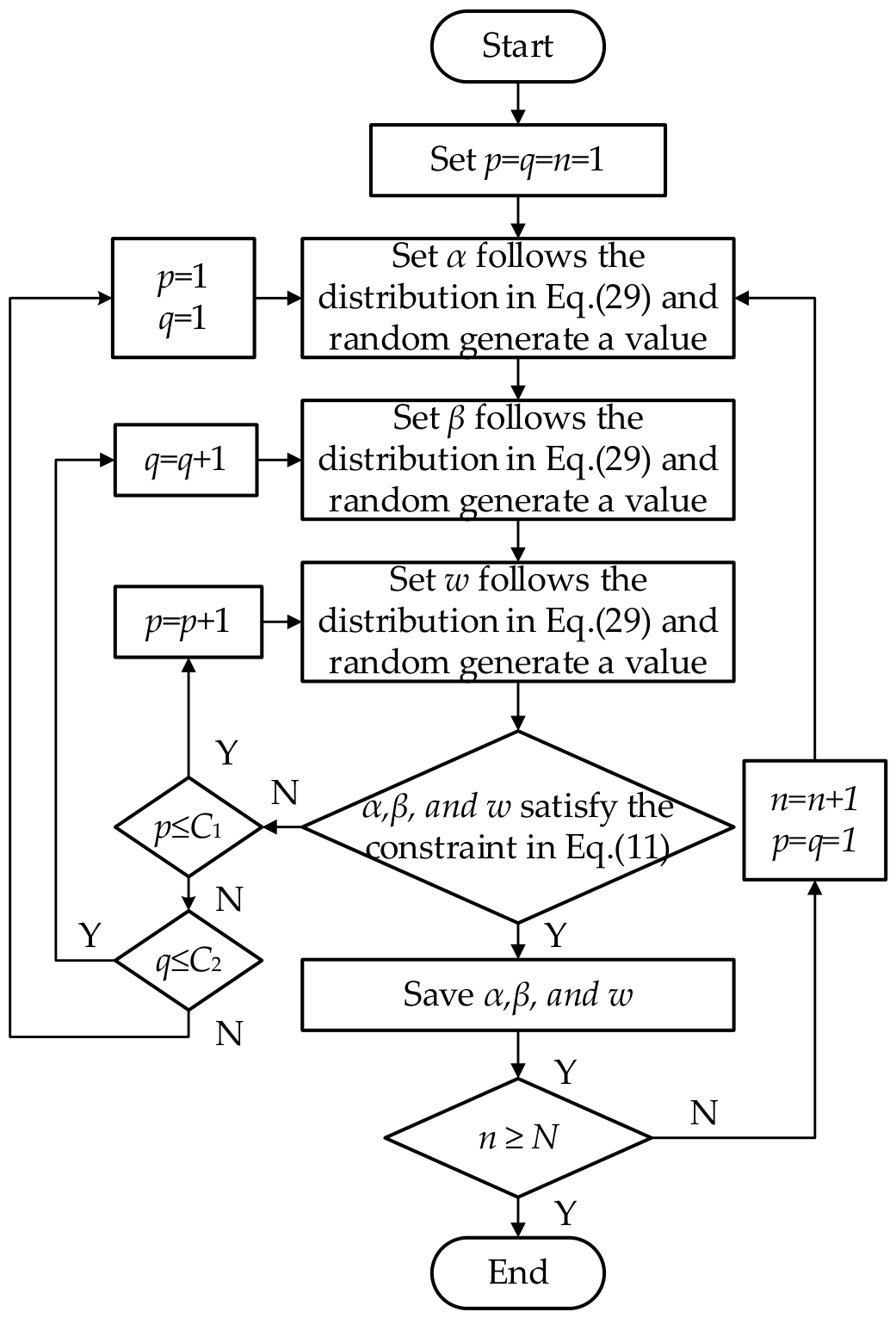
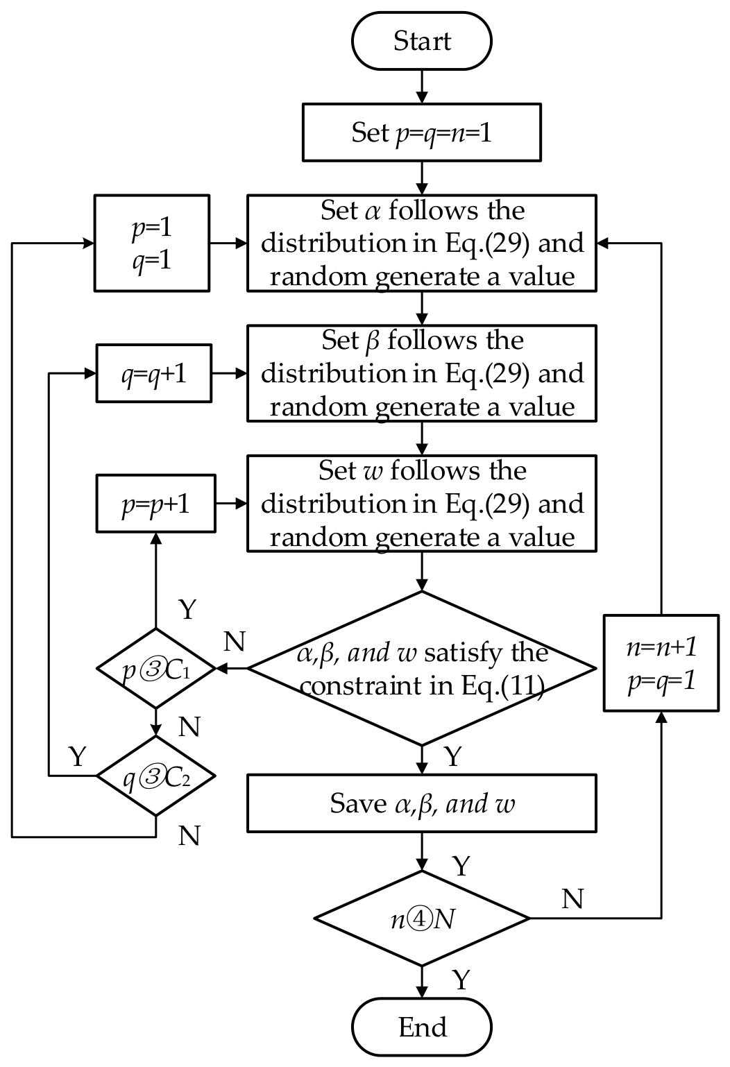
Step 2: Random generation of SDT. Based on the distribution of each torsor parameter in Equation (29), they are randomly generated according to the procedure illustrated in Figure 8.

Step 3: Constraint checking. For generated torsors, it is checked whether they satisfy the constraint conditions in Equation (11). If not, the torsor is regenerated until the constraint is satisfied.

Step 4: Iteration. Steps (2) and (3) are repeated until a sufficient number of torsors satisfying the constraints is obtained.

In Figure 8, n denotes the n-th major loop. In each major loop, one set of SDT parameter is randomly sampled, and a total of N sets are obtained. The variables p and q represent the sampling counts for w and β, respectively, within one major loop. When these counts exceed the constants C₁ and C₂, it indicates that the previously sampled parameter values are too extreme to yield values satisfying the constraints, leading to an infinite loop. In such cases, the previous parameters would be resampled. Furthermore, the random sampling order of the SDT is α → β → γ. To ensure that the sampling order does not affect the final results, sampling should be conducted for each possible order. For three SDT parameters, six possible sampling orders exist, yielding a total of 6N sets of SDT parameters.

To quantitatively evaluate the computational efficiency and numerical robustness of the MCS procedure under the constraint Equation (11), the sample acceptance rate η was monitored. For the base upper surface, generating 10,000 valid SDT parameter sets required a total of 37,570 trial evaluations, yielding an acceptance rate of η = 26.62%. This indicates that an average of only 3.76 sampling trials is required to obtain one valid parameter set. Generating the complete valid dataset required 0.48 s on a standard personal computer. The acceptance rate of 26.62% indicates that the constraint does not lead to excessive sample rejection and that the proposed sampling procedure remains computationally feasible under the specified tolerance conditions.

Similarly, for the SDT (0, β, γ, 0, v, w) of the guideway–slider system, they are assumed to follow normal distributions:

$$\left\{\begin{array}{c}\begin{array}{c}\beta ~N(0,{({\displaystyle \frac{T_4}{6l}})}^2)\\ \gamma ~N(0,{({\displaystyle \frac{T_5}{6l}})}^2)\\ v~N(0,{({\displaystyle \frac{T_5}{6}})}^2)\end{array}\\ w~N(0,{({\displaystyle \frac{T_4}{6}})}^2)\end{array}\right.$$

(30)

The SDT of the guideway–slider system is generated following the same procedure, producing 6N sets of SDT, as well.

4.2. Error Prediction Based on Error Propagation Model

The generated SDTs are substituted into Equations (18)–(21). Based on the error propagation model from the base to the sliders, 6N sets of SDT (α^s, β^s, γ^s, u^s, v^s, w^s) for the four sliders are obtained. These are then substituted into Equation (27) to compute 6N sets of SDT (α_o, β_o, γ_o, u_o, v_o, w_o) for the worktable based on the error propagation model from the four sliders to the worktable.

Although the SDT parameters randomly sampled according to Equation (29) follow normal distributions, the actual distribution types of the worktable SDT may change due to the satisfaction of constraint conditions and the subsequent error propagation calculations. Therefore, it is necessary to test the actual distribution types of the final worktable SDT. If the worktable SDT (α_o, β_o, γ_o, u_o, v_o, w_o) follows a normal distribution, the maximum likelihood estimation method is applied to estimate the mean ${\widehat{\mu }}_x$ and standard deviation ${\widehat{\sigma }}_x$ of each SDT parameter based on the 6N samples:

$$\left\{\begin{array}{cc}\begin{array}{l}{\widehat{\mu }}_x={\displaystyle \frac{1}{6N}}{\displaystyle \sum _{t=1}^{6N}{x}_t}\\ {\widehat{\sigma }}_x=\sqrt{{\displaystyle \frac{1}{6N}}{\displaystyle \sum _{t=1}^{6N}{(x_t-{\widehat{\mu }}_x)}^2}}\end{array}& (x={\alpha }_{\mathrm{o}},{\beta }_{\mathrm{o}},{\gamma }_{\mathrm{o}},u_{\mathrm{o}},v_{\mathrm{o}},w_{\mathrm{o}})\end{array}\right.$$

(31)

where x_t is the t-th sample value of a particular worktable SDT.

Taking the maximum likelihood estimates as the parameters of the normal distribution for (α_o, β_o, γ_o, u_o, v_o, w_o), the confidence interval at the 99.73% confidence level is $({\widehat{\mu }}_x-3{\widehat{\sigma }}_x,{\widehat{\mu }}_x+3{\widehat{\sigma }}_x)$. Accordingly, the actual variation interval width of the worktable error can be considered as:

$$\begin{array}{cc}{W}_x=6{\widehat{\sigma }}_x& (x={\alpha }_{\mathrm{o}},{\beta }_{\mathrm{o}},{\gamma }_{\mathrm{o}},u_{\mathrm{o}},v_{\mathrm{o}},w_{\mathrm{o}})\end{array}$$

(32)

5. Case Study

A linear axis with specified tolerance design parameters is considered as a case study to demonstrate the application of the proposed error prediction method. The structure of the linear axis is shown in Figure 1, and its tolerance values are specified as follows: T₁ = T₃ = 10 μm, T₂ = 20 μm, and T₄ = T₅ = 12 μm. The length, width, and height of the base are a = 4100 mm, b = 320 mm, and c = 120 mm, respectively. The length, width, and height of the guideway–slider system are l = 4000 mm, m = 50 mm, and h = 36 mm, respectively. The installation dimension between the four sliders is D_x = 196 mm in the X-direction and D_y = 180 mm in the Y-direction.

5.1. Random Generation of SDT

Following the procedure illustrated in Figure 8, the parameters are set as N = 10,000, C₁ = 5, and C₂ = 5. The MCS is applied to generate SDT for three geometric features: the lower base surface, the upper base surface, and the travel line of the guideway–slider system. These torsors follow normal distributions within their respective error variation ranges and satisfy the corresponding constraint conditions. Their distribution parameters are as follows:

$$\left\{\begin{array}{l}{\alpha }_1~N(0,{({\displaystyle \frac{T_1}{6b}})}^2)\\ {\beta }_1~N(0,{({\displaystyle \frac{T_1}{6a}})}^2)\\ w_1~N(0,{({\displaystyle \frac{T_1}{6}})}^2).\end{array}\right. \left\{\begin{array}{l}{\alpha }_2~N(0,{({\displaystyle \frac{T_2+T_3}{6b}})}^2)\\ {\beta }_2~N(0,{({\displaystyle \frac{T_2+T_3}{6a}})}^2)\\ w_2~N(0,{({\displaystyle \frac{T_3}{6}})}^2).\end{array}\right. \left\{\begin{array}{l}{\beta }_3^g~N(0,{({\displaystyle \frac{T_4}{6l}})}^2)\\ {\gamma }_3^g~N(0,{({\displaystyle \frac{T_5}{6l}})}^2)\\ v_3^g~N(0,{({\displaystyle \frac{T_5}{6}})}^2)\\ w_3^g~N(0,{({\displaystyle \frac{T_4}{6}})}^2)\end{array}\right.$$

(33)

For each of the above torsors, a total of 6N = 60,000 samples are obtained.

5.2. Determination of the Four-Slider SDT

The error propagation from the base to the four sliders is calculated using Equations (18)–(21), yielding 6N sets of SDT parameters (α^s, β^s, γ^s, u^s, v^s, w^s) for each slider (s = 1, 2, 3, 4).

5.3. Determination of Worktable SDT from Four-Slider SDT

The transfer coefficients $K_j^{si}$ from the SDT parameter i (i = α, β, γ, u, v, w) of slider s to the worktable SDT parameter j (j = α, β, γ, u, v, w) are determined via FEA. Then, the final worktable SDT (α_o, β_o, γ_o, u_o, v_o, w_o) are calculated by transfer coefficients $K_j^{si}$ and the four-slider SDT (α^s, β^s, γ^s, u^s, v^s, w^s).

5.3.1. Construction and Analysis of the Worktable Finite Element Model

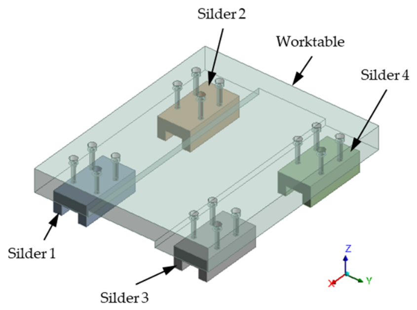
A simplified three-dimensional model of the sliders and the worktable was constructed, as shown in Figure 9. The model consists of four sliders and the worktable. The contact surfaces between the sliders and the guiderails are simplified as planes, and each contact surface is coupled to the geometric center point of the corresponding surface. The slider errors are applied as displacement loads at these center points to maximize computational efficiency. This simplification is consistent with the physical mechanism of error propagation from the sliders to the worktable. Specifically, before the four sliders are connected to the worktable, the errors of each slider originate from the geometric errors of the guiderail raceway surfaces. After connection, the errors of the four sliders are propagated to the worktable through the four bolted interfaces and interact with each other. Therefore, simplifying the slider errors as displacement loads applied at the geometric centers of the contact surfaces (i.e., the centers of the guiderail raceway surfaces) is reasonable and provides an appropriate approximation for the subsequent error mapping analysis.

The material for both the sliders and the worktable is specified as structural steel, with the performance parameters listed in

Table 3. The performance parameters of structural steel.

Parameters	Density (kg/m3)	Young’s Modulus (MPa)	Poisson’s Ratio
Value of structural steel	7850	210,000	0.3

. All structures are meshed with tetrahedral elements, with the element sizes specified in

Table 4. Mesh element sizes.

Geometric Structure	Sliders	Worktable	Mounting Hole Faces
Element size	5 mm	7 mm	3 mm

.

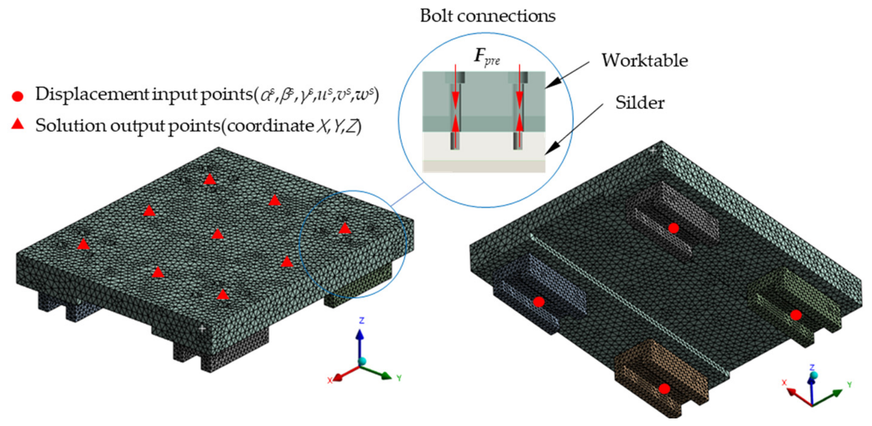
The boundary conditions are configured as shown in Figure 10. At each displacement input point, three rotational and three translational displacements (α^s, β^s, γ^s, u^s, v^s, w^s) are applied. The input point is coupled to the contact surface between the slider and the guiderail. The displacement magnitudes should remain within the slider SDT variation ranges defined in Section 3.3.2. A bolt preload F_pre is applied at the mounting holes between the sliders and the worktable, with its magnitude set to the recommended preload for bolts of 6 mm diameter and property class 10.9 [42].

The solution outputs include the X, Y, and Z directional deformations at nine points on the upper surface of the worktable, as shown in Figure 10. Based on these nine points, an error plane is fitted using the least-squares method. The deviation of this plane from the nominal position of the worktable yields the worktable SDT parameters (α_o, β_o, γ_o, u_o, v_o, w_o).

5.3.2. Solution of Transfer Coefficients

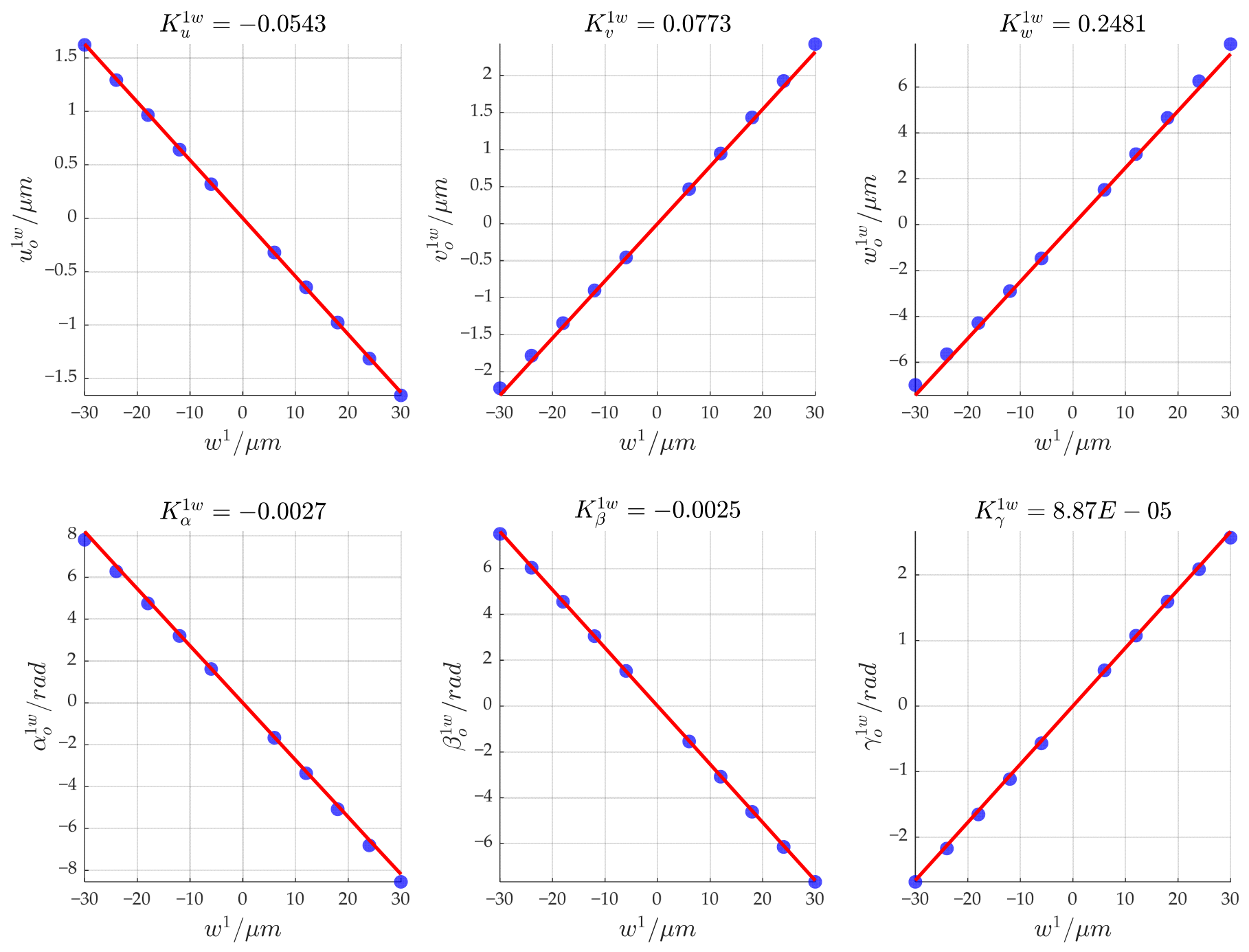
Taking the 24 SDT parameters of the four sliders as inputs and the six SDT parameters of the worktable as outputs, the transfer coefficients are determined following the procedure described in Section 3.3.3. Specifically, a single SDT input of a particular slider is varied incrementally within the slider SDT variation ranges, and FEA is performed sequentially for each variation case. Taking the variation of the Z-direction translational error w¹ of Slider 1 as an example,

Table 5. FEA results of the worktable SDT under w¹ variations.

Sliders SDT (αs/rad, βs/rad, γs/rad, us/μm, vs/μm, ws/μm)				Worktable SDT
Slider 1	Slider 2	Slider 3	Slider 4	(${\alpha }_o^{1w}$/rad,${\beta }_o^{1w}$/rad,${\gamma }_o^{1w}$/rad,$u_o^{1w}$/μm,$v_o^{1w}$/μm,$w_o^{1w}$/μm)
(0,0,0,0,0,−30)	(0,0,0,0,0,0)	(0,0,0,0,0,0)	(0,0,0,0,0,0)	(7.799 × 10−5, 7.514 × 10−5, −2.683 × 10−6, 1.622, −2.221, −6.989)
(0,0,0,0,0,−24)	(0,0,0,0,0,0)	(0,0,0,0,0,0)	(0,0,0,0,0,0)	(6.285 × 10−5, 6.039 × 10−5, −2.173 × 10−6, 1.293, −1.782, −5.648)
(0,0,0,0,0,−18)	(0,0,0,0,0,0)	(0,0,0,0,0,0)	(0,0,0,0,0,0)	(4.754 × 10−5, 4.554 × 10−5, −1.653 × 10−6, 0.966, −1.342, −4.288)
(0,0,0,0,0,−12)	(0,0,0,0,0,0)	(0,0,0,0,0,0)	(0,0,0,0,0,0)	(3.200 × 10−5, 3.052 × 10−5, −1.114 × 10−6, 0.642, −0.900, −2.897)
(0,0,0,0,0,−6)	(0,0,0,0,0,0)	(0,0,0,0,0,0)	(0,0,0,0,0,0)	(1.620 × 10−5, 1.533 × 10−5,−5.692 × 10−7, 0.319, −0.455, −1.472)
(0,0,0,0,0,6)	(0,0,0,0,0,0)	(0,0,0,0,0,0)	(0,0,0,0,0,0)	(−1.664 × 10−5, −1.540 × 10−5,5.443 × 10−7, −0.320, 0.467, 1.522)
(0,0,0,0,0,12)	(0,0,0,0,0,0)	(0,0,0,0,0,0)	(0,0,0,0,0,0)	(−3.361 × 10−5, −3.078 × 10−5,1.075 × 10−6, −0.646, 0.945, 3.079)
(0,0,0,0,0,18)	(0,0,0,0,0,0)	(0,0,0,0,0,0)	(0,0,0,0,0,0)	(−5.075 × 10−5, −4.611 × 10−5, 1.595 × 10−6, −0.976, 1.432, 4.658)
(0,0,0,0,0,24)	(0,0,0,0,0,0)	(0,0,0,0,0,0)	(0,0,0,0,0,0)	(−6.806 × 10−5, −6.139 × 10−5, 2.088 × 10−6, −1.313, 1.925, 6.258)
(0,0,0,0,0,30)	(0,0,0,0,0,0)	(0,0,0,0,0,0)	(0,0,0,0,0,0)	(−8.549 × 10−5, −7.666 × 10−5, 2.570 × 10−6, −1.657, 2.424, 7.874)

presents the FEA results of the worktable SDT under this condition.

Based on the data in Table 5, the transfer coefficients K (j = α, β, γ, u, v, w) from the Z-direction translational error w¹ of Slider 1 to the six worktable SDT parameters are obtained through linear fitting, as shown in Figure 11 and Equation (34).

$$K_j^{1w}=[\begin{array}{llllll}-0.0027\hfill & -0.0025\hfill & 8.87\times {10}^{-5}\hfill & -0.0543\hfill & 0.0773\hfill & 0.2481]\hfill \end{array}$$

(34)

Following the same procedure, all 144 transfer coefficients $K_j^{si}$ from SDT parameters i (i = α, β, γ, u, v, w) of slider s to worktable SDT parameters j (j = α, β, γ, u, v, w) are determined, with the results summarized in

Table 6. The result of all error transfer coefficients $K_j^{si}$ from sliders to worktable.

s	i	j
		α	β	γ	u	v	w
1	α	0.0036	−0.0196	−0.0310	−0.2752	−6.4655	2.3322
	β	−0.0403	−0.0050	0.0426	8.3017	0.4703	3.9643
	γ	−6.91 × 10−4	−8.36 × 10−4	0.0097	−0.1126	−0.3831	−0.1443
	u	1.74 × 10−4	1.34 × 10−6	0.0013	0.2471	−0.0125	−0.0176
	v	3.96 × 10−7	−2.98 × 10−4	0.0012	−0.0071	0.2347	0.0343
	w	−0.0027	−0.0025	8.87 × 10−5	−0.0543	0.0773	0.2481
2	α	0.0035	0.0200	0.0324	0.2863	−6.6585	2.3440
	β	0.0405	−0.0050	0.0435	8.4049	−0.5876	−3.9430
	γ	6.84 × 10−4	−8.47 × 10−4	0.0098	−0.1240	0.3778	0.1503
	u	−1.71 × 10−4	4.45 × 10−7	0.0013	0.2508	0.0089	0.0188
	v	2.61 × 10−6	2.91 × 10−4	−0.0012	0.0067	0.2405	0.0345
	w	−0.0027	0.0025	−8.91 × 10−5	0.0544	0.0764	0.2485
3	α	0.0036	0.0197	−0.0322	0.3007	−6.6756	−2.3108
	β	0.0405	−0.0052	−0.0447	8.6436	−0.4957	3.9594
	γ	−7.24 × 10−4	8.64 × 10−4	0.0099	0.1235	−0.4278	0.1569
	u	−1.72 × 10−4	−9.83 × 10−7	−0.0014	0.2576	0.0124	−0.0186
	v	2.21 × 10−7	2.96 × 10−4	0.0012	0.0059	0.2416	−0.0353
	w	0.0027	−0.0025	−8.87 × 10−5	−0.0540	−0.0775	0.2485
4	α	0.0035	−0.0198	0.0307	−0.3000	−6.3289	−2.3422
	β	−0.0404	−0.0051	−0.0413	7.9968	0.5682	−3.9639
	γ	6.54 × 10−4	7.94 × 10−4	0.0092	0.1082	0.3557	−0.1410
	u	1.70 × 10−4	−4.53 × 10−7	−0.0013	0.2380	−0.0089	0.0175
	v	2.31 × 10−6	−2.90 × 10−4	−0.0011	−0.0061	0.2298	−0.0335
	w	0.0027	0.0025	8.89 × 10−5	0.0539	−0.0762	0.2479

.

5.3.3. Solution of Worktable SDT

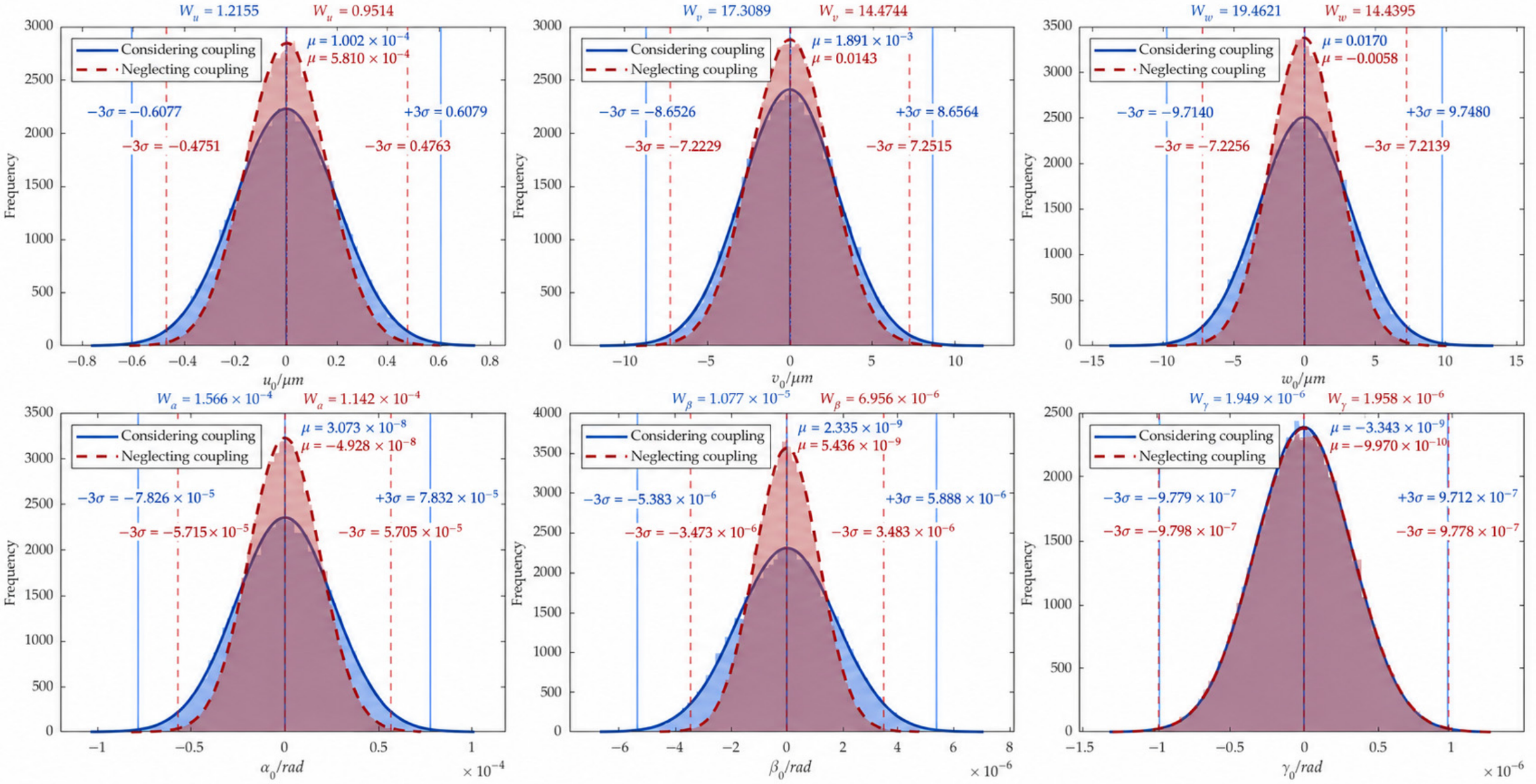
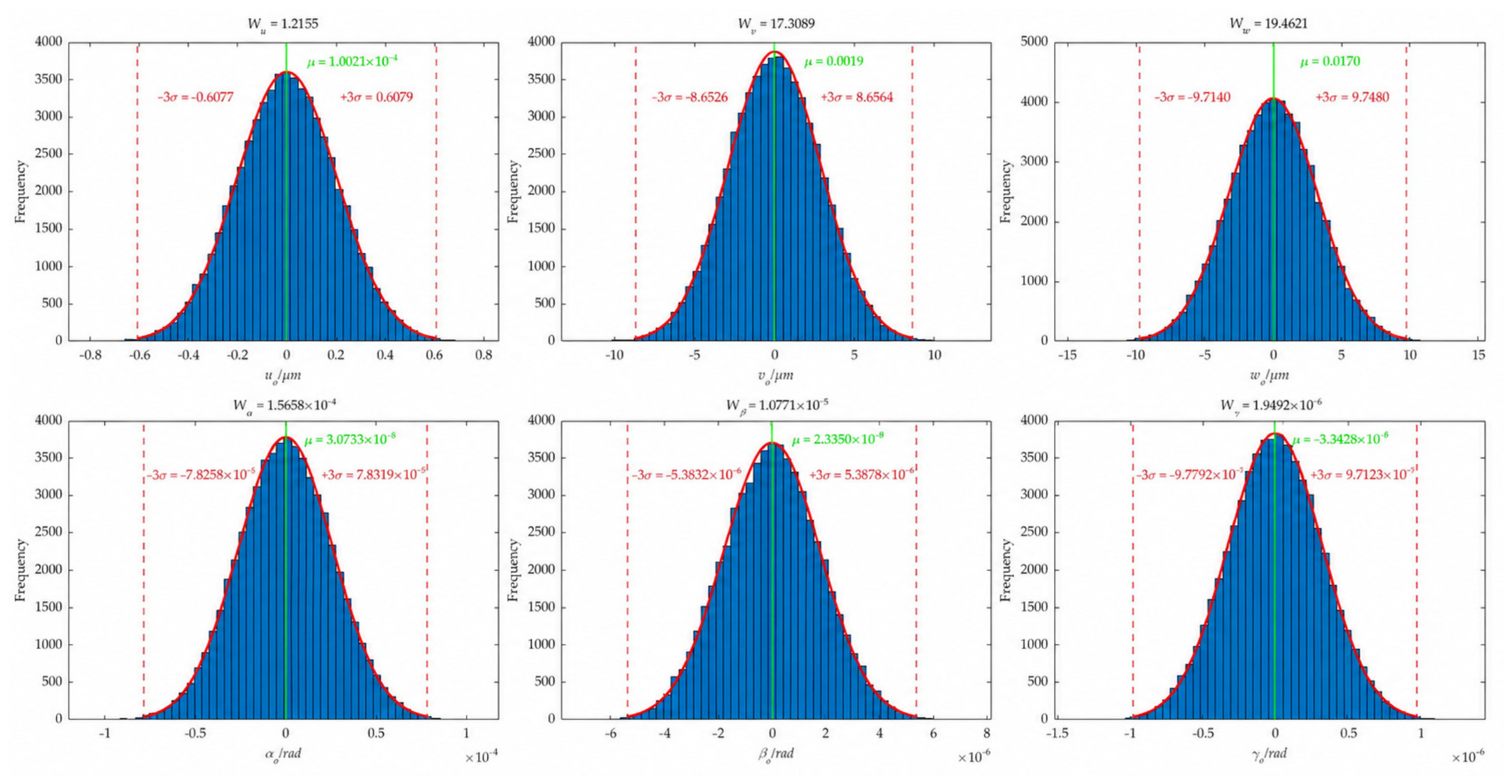
Substituting all transfer coefficients listed in Table 6 and the four-slider SDT obtained in Section 5.2 into Equations (26) and (27), the final worktable SDT are calculated. Figure 12 presents the MCS results for the six SDT parameters of the worktable. All parameters follow normal distributions, with their means close to zero. Subsequently, the variation interval width W_x of each SDT parameter is calculated using Equations (31) and (32), which characterizes the magnitude of the SDT variation range.

5.4. Comparative Evaluation and Prediction Risk Analysis

At the preliminary tolerance design stage, experimental evaluation across a large number of stochastic tolerance combinations is generally impractical. Therefore, this section focuses on method-based comparative evaluation and quantitatively examines the prediction risks associated with simplified assumptions. The comparative evaluations are conducted from two distinct perspectives: (1) whether worktable elastic deformation is considered, and (2) whether tolerance coupling is considered.

5.4.1. Comparison of Considering vs. Neglecting Worktable Elastic Deformation

This subsection compares the error prediction results obtained by the proposed method (considering worktable elastic deformation) and a simplified method (rigid-body assumption) under MCS. Based on the four-slider SDT (α^s, β^s, γ^s, u^s, v^s, w^s), the simplified method assumes that the worktable is a rigid body and calculates its SDT by geometric averaging or differencing as Equation (22).

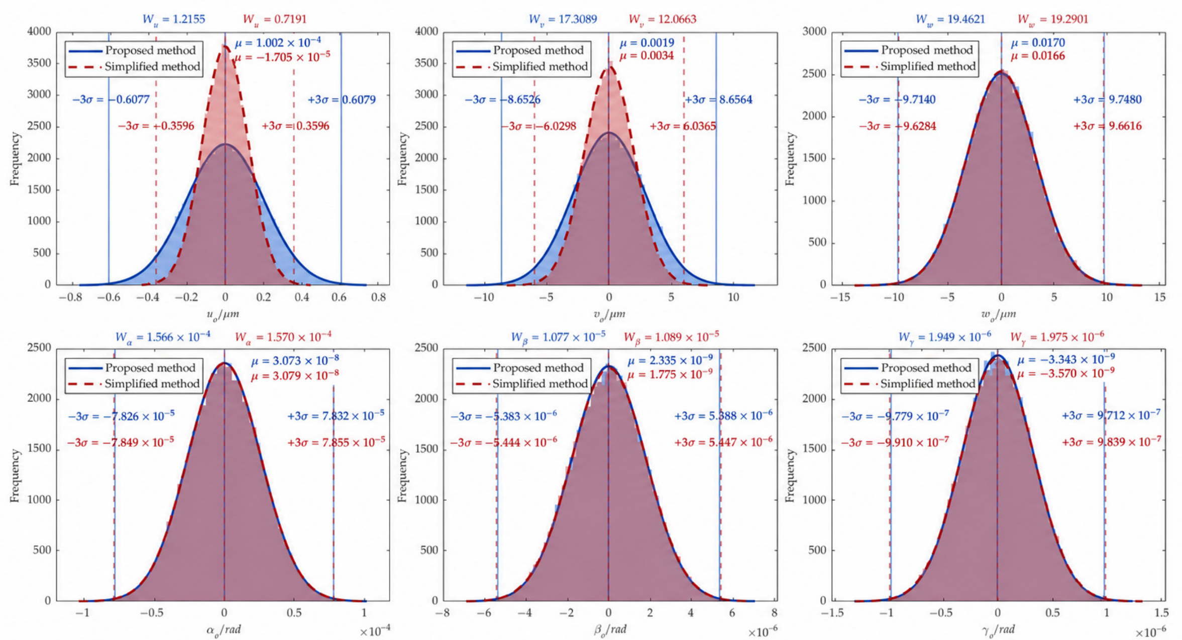
The MCS results obtained using the simplified and proposed methods are presented in Figure 13. The comparison reveals that whether worktable elastic deformation is considered has no effect on the means μ of the six worktable SDT parameters. The means are close to zero in both methods because the slider error variation ranges are symmetric about zero in both cases, and considering the elastic deformation of worktable does not introduce any systematic bias. Regarding the standard deviations σ of the six SDT parameters, the results for α_o, β_o, γ_o and w_o obtained by the proposed method are nearly identical to those from the simplified method. In contrast, the results for u_o and v_o are significantly larger than those from the simplified method.

The reasons for these differences are as follows.

The torsors α_o, β_o, and w_o are primarily influenced by the w^s of the four sliders (as can be seen from the transfer coefficients obtained via FEA in Table 6), and the transfer coefficient values are highly similar to Equation (22) of the simplified method (e.g., w_o is predominantly affected by w^s of the four sliders, with transfer coefficients of approximately 0.25). Meanwhile, γ_o is also primarily influenced by u^s and v^s, and its transfer coefficients are also similar to Equation (22). Consequently, the differences in α_o, β_o, γ_o and w_o between the two methods are minor. In contrast, for u_o and v_o, Table 6 shows that they are not only influenced by u^s and v^s of the four sliders (with transfer coefficients of approximately 0.25) but are also affected by w^s (with transfer coefficients of approximately ±0.054). The simplified method, however, only accounts for slider errors in the corresponding directions and neglects the contributions of errors in other directions, thereby leading to an underestimation of the worktable errors.

The above results indicate that the simplified method (neglecting worktable elastic deformation) leads to optimistic estimates of the worktable errors. Specifically, the variation interval widths W_uo and W_vo are underestimated by approximately 40% and 30%, respectively. Therefore, relying on the rigid-body assumption of worktable poses a potential risk in linear axis error prediction. For applications with high precision requirements, the effect of worktable elastic deformation should be incorporated to obtain reliable error predictions.

5.4.2. Comparison of Considering vs. Neglecting Tolerance Coupling

This subsection compares the error prediction results obtained by considering tolerance coupling (the result is the same as that of the proposed method) and neglecting tolerance coupling under MCS. Based on the original tolerance design values in the case study, if tolerance coupling is neglected in the analysis, the parallelism tolerance T₂ between the upper and lower base surfaces is excluded from the analysis, meaning that the upper base surface is subject only to the flatness tolerance T₃. In this case, the SDT variation range of the upper base surface changes, and the Monte Carlo sampling distribution is correspondingly adjusted to:

$$\left\{\begin{array}{l}{\alpha }_2~N(0,{({\displaystyle \frac{T_3}{6b}})}^2)\\ {\beta }_2~N(0,{({\displaystyle \frac{T_3}{6a}})}^2)\\ w_2~N(0,{({\displaystyle \frac{T_3}{6}})}^2)\end{array}\right.$$

(35)

The MCS results of considering tolerance coupling and neglecting tolerance coupling are presented in Figure 14.The results show that considering coupling has no effect on the means μ of the six worktable SDT parameters. The means are close to zero in both methods because tolerance coupling only enlarges the variation ranges of the geometric feature SDT without changing their symmetry and thus introduces no systematic bias in the sample means. However, for the standard deviations σ of the six SDT parameters, the results obtained with tolerance coupling are consistently greater than or equal to those without coupling. This is because coupling enlarges the variation ranges of α₂, β₂, and w₂ on the upper base surface, leading to a higher probability of propagating larger errors to the worktable during simulation, which ultimately results in a generally larger worktable SDT.

It is noteworthy that the standard deviation of γ_o remains nearly identical regardless of whether coupling is considered, making it the only parameter insensitive to tolerance coupling. This is because γ_o is predominantly governed by the translational errors u^s and v^s of sliders (as can be seen from the transfer coefficients in Table 6). Since tolerance coupling only enlarges the variation ranges of α₂, β₂, and w₂ on the upper base surface and has a negligible effect on the u^s and v^s, it does not influence γ_o.

The above results indicate that neglecting tolerance coupling leads to overly optimistic error predictions. For α_o, β_o, u_o, v_o, and w_o, the optimistic estimates reduce the variation interval widths W_αo, W_βo, W_uo, W_vo, and W_wo by approximately 28%, 43%, 22%, 17%, and 25%, respectively. This underestimates the tolerance-induced uncertainty of the predicted errors and may increase the risk of the linear axis failing to satisfy the specified accuracy requirements. Therefore, tolerance coupling should be incorporated into error prediction to improve the reliability of the prediction results.

5.5. Application of the Proposed Method in Tolerance Allocation

The ultimate goal of establishing an error prediction model is to guide the rational optimization of component tolerances. As demonstrated in Section 5.4, reliance on simplified models may lead to optimistic bias in the predicted error variation. If such biased models are used to guide tolerance allocation, the resulting allocation schemes may underestimate the required component precision and therefore increase the risk of failing to meet the prescribed accuracy requirements.

In high-precision engineering applications, the translational error u_o along the X-direction is typically guaranteed by the drive system (e.g., ball screw precision) and can be effectively mitigated through software compensation. Therefore, the primary objective of tolerance allocation is to restrict the uncompensated errors—namely, the translational errors (v_o, w_o) and the rotational errors (α_o, β_o, γ_o)—within stringent limits. Assume a precision linear axis requires the variation interval widths of these five uncompensated error parameters to be strictly controlled within a set of target limits W_req = {W_{α_req}, W_{β_req}, W_{γ_req}, W_{v_req}, W_{w_req}}. Specifically, the limits are set as {1.2 × 10⁻⁴ rad, 8 × 10⁻⁶ rad, 1.7 × 10⁻⁶ rad, 12 μm, 14 μm}, respectively.

Based on the initial tolerance design scheme, the predicted errors as shown in Figure 12 do not satisfy these stringent requirements. To achieve the allocation targets without altering the original design tolerance proportions, a uniform scaling factor f is applied to tighten the initial component tolerances T₁–T₅. In addition, to demonstrate the indispensability of the proposed method in tolerance allocation, three different tolerance allocation schemes are derived based on the three different prediction models discussed previously. The scaling factor f for each scheme is determined by the critical error parameter that first reaches its corresponding limit in W_req:

Scheme I (Allocated via Model Neglecting Worktable Elastic Deformation): Driven by this simplified model, a moderately relaxed scaling factor f_I = 0.72 is calculated, falsely indicating that tightening the initial tolerances to 72% is sufficient to meet all targets.

Scheme II (Allocated via Model Neglecting Tolerance Coupling): Driven by this simplified model, a highly relaxed scaling factor f_II = 0.82 is calculated, falsely indicating that tightening the initial tolerances to 82% is sufficient to meet all targets.

Scheme III (Allocated via the Proposed Model): Comprehensively considering both worktable elastic deformation and tolerance coupling, the proposed model strictly demands a scaling factor of f_III = 0.68 to guarantee all five targets are met simultaneously.

To compare the robustness of the three allocation schemes, a model-based verification is conducted. The allocated tolerances from Scheme I, II, and III are respectively substituted back into the proposed model to simulate the error outcomes considering both tolerance coupling and worktable elastic deformation. The verified results are summarized in

Table 7. Comparison of tolerance allocation schemes and the verified error variation interval widths.

Tolerance Allocation Scheme	Scaling Factor	Design Tolerances			Verified Error Variation Interval Widths
	f	T1, T3/μm	T2/μm	T4, T5/μm	Wαo/rad	Wβo/rad	Wγo/rad	Wvo/μm	Wwo/μm
Target Limits (Wreq)	-	-	-	-	1.2 × 10−4	8 × 10−6	1.7 × 10−6	12	14
Initial Scheme	1	10	20	12	1.57 × 10−4	1.08 × 10−5	1.95 × 10−6	17.31	19.46
Scheme I	0.72	7.2	14.4	8.6	1.13 × 10−4	7.79 × 10−6	1.43 × 10−6	12.54	13.97
Scheme II	0.82	8.2	16.4	9.8	1.29 × 10−4	8.83 × 10−6	1.61 × 10−6	14.31	15.86
Scheme III	0.68	6.8	13.6	8.2	1.07 × 10−4	7.33 × 10−6	1.33 × 10−6	11.86	13.22

.

As shown in Table 7, tolerance allocation schemes I and II guided by simplified models may lead to design schemes that fail to satisfy the specified accuracy requirements. The allocation in Scheme I results in violation of the target limit (W_vo = 12.54 > 12 μm), which is consistent with the finding in Section 5.4 that neglecting worktable elastic deformation underestimates the actual translational error v_o. The consequences are even more severe for Scheme II. Because neglecting tolerance coupling underestimates multiple error parameters, the model provides a dangerously loose allocation (f_II = 0.82). Consequently, during verification, W_αo, W_βo, W_vo, and W_wo simultaneously violate their target limits. Notably, W_γo is the only one that satisfies the target in Scheme II, which corroborates the earlier conclusion that the error γ_o is insensitive to tolerance coupling. In contrast, only Scheme III, allocated based on the proposed comprehensive model, successfully restricts all five spatial geometric errors within the target design limits.

Therefore, compared to simplified approaches, the proposed method provides a more physically complete basis for tolerance allocation and reduces the risk of tolerance schemes that underestimate the resulting motion error variation.

5.6. Discussion

5.6.1. Applicability of the Small Deformation Assumption and Sensitivity to Assembly Preload

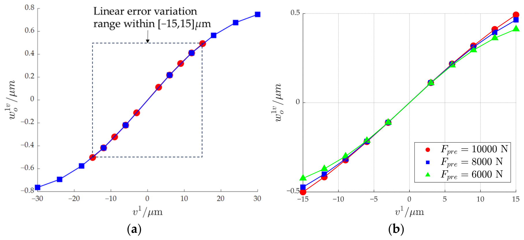
The proposed method relies on the small deformation assumption and the contact linearization of bolted joints. While this treatment decouples complex statically indeterminate interfaces into computationally efficient linear transfer coefficients, its accuracy and physical credibility are inherently governed by the error amplitude and the interface assembly state. To explicitly delineate the range of validity, sensitivity investigations were performed using the response of worktable error parameter $w_o^{1v}$ to the slider 1 translational error parameter v¹ as a representative case, as illustrated in Figure 15.

(1)

Sensitivity to error variation range

Figure 15a examines the influence of the error variation range. Within the range of v¹ in [−15, 15] μm, the worktable error response exhibits approximately linearity. In this range, the micro-scale errors are insufficient to alter the macroscopic compressive state of the contact interfaces, keeping the interfacial stiffness essentially constant. However, when the error is artificially extended to an extreme range of [−30, 30] μm, subtle nonlinear behavior emerges at the curve tails. This nonlinearity stems from the localized redistribution of contact pressure and microscopic stiffness softening under enlarged displacement load. This comparison demonstrates that the linearized contact model provides a physically credible approximation within the investigated error variation range.

(2)

Sensitivity to bolt preloads

Figure 15b illustrates the influence of three distinct bolt preloads: 10,000 N, 8000 N, and 6000 N. At the preload of 10,000 N, the interface operates deep within the contact stiffness saturation regime, yielding optimal linearity and a stable transfer coefficient. As the preload decreases to 8000 N and 6000 N, the departure from linearity initiates at a significantly smaller error amplitude. The reduction in preload degrades the contact stiffnesses of the slider–worktable interface, rendering the assembly more compliant under error excitations.

Consequently, the derived transfer coefficients $K_j^{si}$ (Table 6) are case-specific to the prescribed fastening state. While the analytical methodology (HTM + FEA + MCS) remains universally applicable across various linear axes, the transfer coefficients should be recalibrated via FEA if significant variations in fastener specifications, clamping torque, or structural rigidity occur.

5.6.2. Sensitivity to Alternative Machining Error Distributions

Actual machining errors may exhibit non-normal distributions, such as uniform distributions driven by progressive tool wear or triangular distributions resulting from conservative centering. To assess distributional sensitivity, MCS was conducted across normal, triangular, and uniform distributions under identical error variation ranges and zero means. The resulting variation interval widths W are summarized in

Table 8. Worktable motion error interval widths under different input error distributions.

Distribution	Error Variation Interval Widths					Average Relative Expansion
	Wαo/rad	Wβo/rad	Wγo/rad	Wvo/μm	Wwo/μm
Normal	1.57 × 10−4	1.08 × 10−5	1.95 × 10−6	17.31	19.46	Baseline (0%)
Triangular	1.69 × 10−4	1.13 × 10−5	2.31 × 10−6	18.84	21.47	+8.92%
Uniform	1.83 × 10−4	1.18 × 10−5	2.77 × 10−6	20.44	24.65	+17.73%

.

Owing to the higher variance of the uniform distribution, the output error intervals expand by approximately 17.73%, while the triangular distribution produces a moderate 8.92% increase. Crucially, the underestimation rates caused by neglecting elastic deformation (~40% for W_uo and W_vo) and tolerance coupling (~43% for W_βo) remain practically identical across all distributions. This is because the underestimation mechanisms are structurally governed by the transfer coefficients (Table 6) and error variation ranges rather than the assumed statistical profile.

5.6.3. Physical Consistency of Error Transfer

The FEA-derived transfer coefficients provide a physically interpretable description of the error propagation from the four sliders to the worktable. The direct translational coefficients in Table 6, such as $K_u^{1u}$ = 0.2471, $K_v^{1v}$ = 0.2347, and $K_w^{1w}$= 0.2481, are close to the classical rigid-body averaging coefficient of (1/4 = 0.25), which is consistent with the conventional kinematic formulation in Equation (22). Meanwhile, the proposed model yields non-zero cross-axis coefficients, such as $K_v^{1w}$ = 0.0773, which represent the elastic redistribution of slider errors through the worktable and are not captured by the rigid-body model.

The physical significance of these terms is also consistent with experimental observations reported by Rahmani and Bleicher [28]. In their empirical setup, introducing the Z-direction error w^s of slider directly produced a primary Z-direction error w_o of worktable and an accompanying secondary Y-direction error v_o. Moreover, w^s also influenced the rotational error α_o and β_o of the worktable, while the γ_o remained practically unaffected. This experimental pattern exhibits the same qualitative behavior as the transfer relationships in Table 6, where $K_w^{1w}$ (0.2481) dominates over $K_v^{1w}$ (0.0773), and $K_{\alpha }^{1w},K_{\beta }^{1w}$ exceed the coefficient $K_{\gamma }^{1w}$ by two orders of magnitude.

Further experimental evidence was reported by Sun et al. [36]. Their results also show that Z-direction errors w^s mainly affect the w_o, α_o and β_o of worktable, whereas Y-direction errors v^s mainly affect the v_o and γ_o of the worktable. In addition, Y-direction errors v^s of 3.35 μm in a single guideway produced a primary worktable Y-direction error of 1.66 μm and a secondary Z-direction error of 0.51 μm. Similarly, Z-direction errors w^s of 5.96 μm in a single guideway produced a primary worktable Z-direction error of 2.89 μm and a secondary Y-direction error of 0.51 μm. These observations demonstrate both the directional dominance and cross-axis redistribution of guideway errors, which are similar to the transfer characteristics obtained in Table 6.

Overall, the agreement with the experimentally observed error transfer reported in [28,36] supports the physical interpretation of the FEA-derived transfer relationships and indicates that the proposed model captures transfer mechanisms consistent with those observed in practical linear-guide systems.

5.6.4. Applicability Under Continuous Travel and Operating Conditions

The proposed method is established under a static small deformation assumption. This assumption does not mean that the motion error is evaluated at only one fixed position. In the present tolerance model, the parallelism tolerances T₄ and T₅ are imposed over the complete guideway stroke l = 4000 mm and are therefore used to define the admissible geometric error variations throughout the travel range. Consequently, the predicted error interval represents the tolerance-induced motion error envelope associated with the complete stroke under the specified geometric error boundaries.

The effects of motion load and speed are not explicitly introduced as independent variables in the present model. Instead, the adopted guideway tolerances T₄ and T₅ correspond to the selected guideway precision level, while the rated load and operating speed define the intended service conditions of the guideway. Therefore, the proposed method is primarily intended for geometric motion error prediction of the selected guideway system within its specified operating range. Under such conditions, the model evaluates the influence of geometric tolerance and worktable elastic deformation without additionally introducing load-dependent or speed-dependent dynamic error terms.

When the operating load, acceleration, or speed becomes sufficiently high to cause significant changes in structural deformation, contact conditions, inertia, or vibration, the static transfer coefficients may no longer remain constant. Such effects are beyond the scope of the present model and would require load-dependent and dynamic analyses in future work.

6. Conclusions

This paper proposes a novel method for predicting the motion errors of a linear axis that, unlike existing methods, simultaneously integrates tolerance coupling and worktable elastic deformation into a unified error propagation framework. The method addresses the limitations associated with neglecting multi-tolerance coupling and worktable elastic deformation in conventional simplified models, providing a more reliable tool for precision motion accuracy design.

(1)

An analytical model is established for the SDT variation ranges of geometric features under the coupling of flatness and parallelism tolerances on the base. The derivation results indicate that multi-tolerance coupling enlarges the SDT variation ranges of the upper base surface, thereby affecting the input conditions for subsequent error propagation.

(2)

A two-stage error propagation model is constructed from the base, through the four sliders, to the worktable. In the first stage, HTM is used to describe the series error propagation from the base to the sliders. In the second stage, based on the small deformation assumption and the superposition principle, FEA is employed to determine the transfer coefficients from slider errors to worktable errors. The model accommodates the hybrid propagation path combining both series propagation from base to sliders and parallel mapping from sliders to worktable.

(3)

Through a case study, the proposed method is compared with simplified methods that neglect either worktable elastic deformation or tolerance coupling. The MCS results show that neglecting worktable elastic deformation underestimates u_o and v_o by approximately 30% and 40%, while α_o, β_o, γ_o and w_o are nearly identical to those from the simplified method. Neglecting tolerance coupling leads to underestimations of the variation interval widths of α_o, β_o, u_o, v_o, and w_o by approximately 28%, 43%, 22%, 17%, and 25%, respectively, while γ_o is insensitive to this coupling effect. These substantial underestimations indicate that simplified methods may lead to overconfident accuracy predictions and inadequate tolerance design. A subsequent tolerance-allocation case demonstrates that the simplified models can produce non-conservative allocation schemes because of their systematic underestimation of motion error variation, whereas the proposed comprehensive model provides a more physically complete basis for tolerance allocation.

The proposed method is applicable to quasi-static motion error prediction within the investigated small deformation range and under the specified operating conditions of the selected linear guideway system. Its applicability may be limited when large deformations, significant changes in contact conditions, or pronounced load- and speed-dependent dynamic effects occur. In addition, direct experimental validation of the absolute prediction accuracy for the investigated linear axis is an important direction for future work.

References

1. Zhou, J.; Yu, H.; He, M.; Zhang, Y.; Luan, X.; Liu, Y. Application-oriented classification and performance analysis of precision linear feed mechanisms for machine tools. Sci. Prog. 2026, 109, 368504251410781. [Google Scholar] [CrossRef] [Scilit]
2. Kenno, T.; Sato, R.; Shirase, K.; Natsume, S.; Spaan, H.A.M. Influence of linear-axis error motions on simultaneous three-axis controlled motion accuracy defined in ISO 10791-6. Precis. Eng. 2020, 61, 110–119. [Google Scholar] [CrossRef] [Scilit]
3. Majda, P. Modeling of geometric errors of linear guideway and their influence on joint kinematic error in machine tools. Precis. Eng. 2012, 36, 369–378. [Google Scholar] [CrossRef] [Scilit]
4. Altintas, Y.; Verl, A.; Brecher, C.; Uriarte, L.; Pritschow, G. Machine tool feed drives. CIRP Ann. 2011, 60, 779–796. [Google Scholar] [CrossRef] [Scilit]
5. Skrypnyk, T.; Korenkov, V. Temperature compensation in ball screws of CNC machines. Mech. Adv. Technol. 2025, 9, 157–165. [Google Scholar] [CrossRef] [Scilit]
6. Sun, J.; Zhang, Y.; Ma, X.; Li, B.; Yang, M.; Xu, L.; Xin, H.; An, Q.; Zhu, L.; Bie, Q.; et al. Multi-source errors evaluation of machine tools: From research gaps to methodologies and applications. Int. J. Extrem. Manuf. 2025, 8, 022002. [Google Scholar] [CrossRef] [Scilit]
7. Wang, L.; Han, J.; Tang, Z.; Zhang, Y.; Wang, D.; Li, X. Geometric accuracy design of high performance CNC machine tools: Modeling, analysis, and optimization. Chin. J. Mech. Eng. 2025, 38, 87. [Google Scholar] [CrossRef] [Scilit]
8. Schwenke, H.; Knapp, W.; Haitjema, H.; Weckenmann, A.; Schmitt, R.; Delbressine, F. Geometric error measurement and compensation of machines—An update. CIRP Ann. 2008, 57, 660–675. [Google Scholar] [CrossRef] [Scilit]
9. Zhang, Z.; Jiang, F.; Luo, M.; Wu, B.; Zhang, D.; Tang, K. Geometric error measuring, modeling, and compensation for CNC machine tools: A review. Chin. J. Aeronaut. 2024, 37, 163–198. [Google Scholar] [CrossRef] [Scilit]
10. Greenwood, W.H.; Chase, K.W. Worst case tolerance analysis with nonlinear problems. J. Eng. Ind. 1988, 110, 232–235. [Google Scholar] [CrossRef] [Scilit]
11. Greenwood, W.H.; Chase, K.W. A new tolerance analysis method for designers and manufacturers. J. Eng. Ind. 1987, 109, 112–116. [Google Scholar] [CrossRef] [Scilit]
12. Gao, J.; Chase, K.W.; Magleby, S.P. Comparison of assembly tolerance analysis by the direct linearization and modified monte carlo simulation methods. In Proceedings of the ASME 1995 Design Engineering Technical Conferences, Boston, MA, USA, 17–20 September 1995; pp. 353–360. [Google Scholar]
13. Sepahi-Boroujeni, S.; Mayer, J.R.R.; Khameneifar, F. Efficient uncertainty estimation of indirectly measured geometric errors of five-axis machine tools via monte-carlo validated GUM framework. Precis. Eng. 2021, 67, 160–171. [Google Scholar] [CrossRef] [Scilit]
14. Guo, S.; Yang, J.; Qiao, G.; Mei, X. Assembly deviation modelling to predict and trace the geometric accuracy of the precision motion system of a CNC machine tool. Mech. Mach. Theory 2022, 169, 104687. [Google Scholar] [CrossRef] [Scilit]
15. Li, X.; Li, Z.; Jin, S.; Zhang, J.; Ding, S.; Niu, Z. A novel error equivalence model on the kinematic error of the linear axis of high-end machine tool. Int. J. Adv. Manuf. Technol. 2022, 118, 2759–2785. [Google Scholar] [CrossRef] [Scilit]
16. Zhou, X.; Li, H.; Zhu, H. A novel kinematic accuracy analysis method for a mechanical assembly based on DP-SDT theory. Int. J. Adv. Manuf. Technol. 2018, 94, 4301–4315. [Google Scholar] [CrossRef] [Scilit]
17. Wu, H.; Li, X.; Sun, F.; Zheng, H.; Zhao, Y. Optimization design method of machine tool static geometric accuracy using tolerance modeling. Int. J. Adv. Manuf. Technol. 2022, 118, 1793–1809. [Google Scholar] [CrossRef] [Scilit]
18. Fan, J.; Li, Z.; Pan, R.; Sun, K.; Chen, K. Volumetric error modeling and prediction for machine tools based on key component tolerance. Alex. Eng. J. 2025, 111, 171–180. [Google Scholar] [CrossRef] [Scilit]
19. Niu, P.; Cheng, Q.; Liu, Z.; Chu, H. A machining accuracy improvement approach for a horizontal machining center based on analysis of geometric error characteristics. Int. J. Adv. Manuf. Technol. 2021, 112, 2873–2887. [Google Scholar] [CrossRef] [Scilit]
20. Huang, Y.B.; Fan, K.C.; Lou, Z.F.; Sun, W. A novel modeling of volumetric errors of three-axis machine tools based on abbe and bryan principles. Int. J. Mach. Tools Manuf. 2020, 151, 103527. [Google Scholar] [CrossRef] [Scilit]
21. Wang, S.; He, G.; Zhang, D.; Yang, Y.; Yan, Y.; Song, Y. B-spline curve-based machine tool guide rails geometric accuracy design. Int. J. Mech. Sci. 2025, 301, 110550. [Google Scholar] [CrossRef] [Scilit]
22. Ghie, W.; Laperrière, L.; Desrochers, A. Statistical tolerance analysis using the unified jacobian–torsor model. Int. J. Prod. Res. 2009, 48, 4609–4630. [Google Scholar] [CrossRef] [Scilit]
23. Fan, J.; Wang, P.; Ren, X. A novel sensitivity analysis of translational axis operation considering key component tolerances. Int. J. Adv. Manuf. Technol. 2022, 118, 1255–1268. [Google Scholar] [CrossRef] [Scilit]
24. Du, Z.; Wu, J.; Yang, J. Geometric error modeling and sensitivity analysis of single-axis assembly in three-axis vertical machine center based on jacobian-torsor model. ASCE-ASME J. Risk Uncertain. Eng. Syst. B Mech. Eng. 2018, 4, 031004. [Google Scholar] [CrossRef] [Scilit]
25. Hui, Y.; Mei, X.; Jiang, G.; Zhao, F.; Ma, Z.; Tao, T. Assembly quality evaluation for linear axis of machine tool using data-driven modeling approach. J. Intell. Manuf. 2022, 33, 753–769. [Google Scholar] [CrossRef] [Scilit]
26. Wang, S.; He, G.; Zhang, D.; Chen, F.; Yao, C.; Yan, Y. Innovative design methods for the geometric accuracy of machine tool guide rail oriented to spatial accuracy. J. Manuf. Process. 2024, 119, 483–498. [Google Scholar] [CrossRef] [Scilit]
27. Guo, Z.; Cheng, Q.; Zhang, H.; Niu, P.; Zhang, C.; Liu, Z. Error analysis model and optimization method for guideway assembly based on elastic interaction effects. Appl. Math. Model. 2026, 156, 116774. [Google Scholar] [CrossRef] [Scilit]
28. Rahmani, M.; Bleicher, F. Experimental and numerical studies of the influence of geometric deviations in the performance of machine tools linear guides. Procedia CIRP 2016, 41, 818–823. [Google Scholar] [CrossRef] [Scilit]
29. Tong, V.-C.; Kwon, S.-W.; Hong, S.-W. Modeling of moving table with linear roller guides subjected to geometric errors in guide rails. Int. J. Precis. Eng. Manuf. 2020, 21, 1903–1919. [Google Scholar] [CrossRef] [Scilit]
30. Yan, X.; Liu, Z.; Liu, W.; Zhao, Y.; Cheng, Q.; Cai, Y. A method for predicting and improving the assembly motion accuracy of linear motion systems in precision machine tools. Precis. Eng. 2026, 99, 593–606. [Google Scholar] [CrossRef] [Scilit]
31. Guo, X.; Wang, H.; Sun, G.; Zhang, D.; Su, Z.; Hu, G. An accuracy design method for a linear feed system of machine tools considering the geometric error shape of the guideway. Machines 2026, 14, 82. [Google Scholar] [CrossRef] [Scilit]
32. Dai, S.; Zhao, L.; Liu, X.; Wang, Z.; Ji, Y.; Qiu, L.; Zhang, S.; Tan, J. A novel accuracy allocation method for machine tools: From geometric errors to manufacturing tolerances. Results Eng. 2026, 30, 110071. [Google Scholar] [CrossRef] [Scilit]
33. Xu, Y.; Tian, W.; Lin, Z.; Huang, Z.; Zhang, D. A scraping curve design method of guideway mounting surfaces considering assembly-induced errors. J. Manuf. Process. 2025, 155, 638–654. [Google Scholar] [CrossRef] [Scilit]
34. Wang, T.; Guo, P.; Liu, H.; Meng, X.; Chen, X.; Zhang, S. A novel straightness error prediction method incorporating machining errors of linear guideways. Precis. Eng. 2025, 96, 905–919. [Google Scholar] [CrossRef] [Scilit]
35. Niu, P.; Cheng, Q.; Zhang, T.; Yang, C.; Zhang, Z.; Liu, Z. Hyperstatic mechanics analysis of guideway assembly and motion errors prediction method under thread friction coefficient uncertainties. Tribol. Int. 2023, 180, 108275. [Google Scholar] [CrossRef] [Scilit]
36. Sun, G.; Chen, S.; Sun, M.; Gao, R.; Zhang, D.; Guo, X.; Zhao, J. Research on the error averaging effect of linear feed systems for precision machine tool. Ain Shams Eng. J. 2024, 15, 103101. [Google Scholar] [CrossRef] [Scilit]
37. Bourdet, P. The Concept of Small Displacement Torsor in Metrology; Series on advances in Mathematics for Applied Sciences; World Scientific: Singapore, 1996; Volume 40, pp. 110–122. [Google Scholar]
38. Peng, H.P.; Lu, W.L. Modeling of geometric variations within three-dimensional tolerance zones. J. Harbin Inst. Technol. 2018, 25, 41–49. [Google Scholar] [CrossRef]
39. Liu, Y.; Zhang, G.; Ran, Y. Geometric element error modeling considering multi-tolerance coupling and accuracy prediction of product assembly. J. Chongqing Univ. 2021, 44, 11–19. [Google Scholar]
40. Lu, C.; Liu, Z.; Ai, Y.; Yu, Z. Assembly joint surface error modeling and tolerance optimization in the case of coupled tolerance. J. Mech. Eng. 2015, 51, 108–118. [Google Scholar] [CrossRef] [Scilit]
41. Nigam, S.D.; Turner, J.U. Review of statistical approaches to tolerance analysis. Comput. Aided Des. 1995, 27, 6–15. [Google Scholar] [CrossRef] [Scilit]
42. Yan, X.; Liu, Z.; Zheng, M.; Li, Y.; Wang, Y.; Chen, W. Preload control method of threaded fasteners: A review. Chin. J. Mech. Eng. 2024, 37, 97. [Google Scholar] [CrossRef] [Scilit]
Figure 1. Structure of linear axis.
Machines 14 01083 g001
Figure 2. Key component design tolerances of linear axis: (a) base; (b) guideway–slider system.
Machines 14 01083 g002
Figure 3. Tolerance coupling of flatness and parallelism.
Machines 14 01083 g003
Figure 4. Projection on the XOZ plane when error variation is at its extreme.
Machines 14 01083 g004
Figure 5. Error variation of line.
Machines 14 01083 g005
Figure 6. Overall framework of error propagation for the linear axis.
Machines 14 01083 g006
Figure 7. The verification of the small displacement assumption.
Machines 14 01083 g007
Figure 8. The process of SDT generation based on MCS.
Machines 14 01083 g008
Figure 9. The simplified three-dimensional model of the sliders and the worktable.
Machines 14 01083 g009
Figure 10. Configuration of boundary conditions and solution output.
Machines 14 01083 g010
Figure 11. The error transfer coefficients through linear fitting based on the data in Table 5.
Machines 14 01083 g011
Figure 12. MCS results for the six SDT parameters of the worktable.
Machines 14 01083 g012
Figure 13. The MCS results and comparison of the simplified method and proposed method.
Machines 14 01083 g013
Figure 14. The MCS results and comparison of considering tolerance coupling (proposed method) and neglecting tolerance coupling.
Machines 14 01083 g014
Figure 15. Sensitivity analysis of error transfer from slider 1 to the worktable: (a) Sensitivity to error variation range; (b) Sensitivity to bolt preloads.
Machines 14 01083 g015