Motion-State-Aware Adaptive Multi-Sensor Fusion Localization Using Sliding-Window Incremental Factor Graph Optimization

Abstract

Accurate and real-time localization for unmanned vehicles in complex motion environments is challenged by asynchronous multi-sensor measurements, time-varying measurement quality, and the growing computational burden of long-term factor graph optimization. To address these problems, this study proposes AVFGO, a sliding-window incremental factor graph optimization framework for motion-state-aware adaptive multi-sensor fusion localization. IMU pre-integration is used as the primary state-propagation backbone, while asynchronous LiDAR odometry, AHRS, wheel odometry, and barometer measurements are uniformly represented as factor-graph constraints. A sliding-window marginalization mechanism bounds the optimization scale by retaining historical information as prior factors. A motion-state-aware fusion-rate strategy controls the insertion density of external factors, and a residual-driven vector-wise adaptive weighting model adjusts the covariance of heterogeneous sensors in different measurement dimensions. Field experiments on a GNSS-denied wheeled unmanned vehicle dataset show that AVFGO achieves a 3D position RMSE of 0.380 m, reducing the error by 65.36% relative to IFGO and 52.71% relative to SWIFGO. The mean single-step optimization time is 0.0389 s, corresponding to an 11.9× speedup over IFGO and a 75.81% reduction relative to SWIFGO. These results indicate that the proposed framework improves accuracy and real-time performance while remaining limited by the single-platform field-test scope, which is explicitly discussed as a direction for future validation.

1. Introduction

Continuous, reliable, and seamless high-precision localization is essential for unmanned inspection, rescue, and other intelligent mobile systems operating in complex environments. This requirement places stringent demands on the robustness, real-time performance, and environmental adaptability of navigation and localization technologies [1]. A single sensor is usually unable to provide stable and reliable pose information over long periods in complex scenarios. Inertial navigation systems are autonomous, have high output rates, and provide accurate short-term motion information, but their errors accumulate over time. GNSS can provide stable absolute positioning in open-sky environments; however, in urban canyons, tunnels, indoor and underground spaces, and environments with strong electromagnetic interference, it is vulnerable to multipath effects, signal blockage, and outages [2,3]. Multi-sensor fusion has therefore become a common solution for mobile robots and intelligent inspection platforms. Navigation sensors differ in sampling rate, measurement accuracy, observability, and failure mode, and their measurements usually arrive asynchronously. In addition, environmental changes and vehicle motion states cause sensor reliability to vary significantly over time. A multi-sensor fusion localization system should therefore support flexible sensor integration and asynchronous measurement processing, while adaptively selecting appropriate fusion strategies according to the current operating state [4]. Lynen et al. [5] proposed a robust modular filtering framework for multi-sensor fusion that handles delayed and asynchronous measurements. However, filtering methods often propagate delayed measurements to the current fusion epoch, which may introduce additional extrapolation errors. Moreover, recursive filtering marginalizes historical states and mainly relies on current innovations, making it difficult to fully exploit correlations among historical observations and obtain globally consistent estimates [6]. Factor graph optimization (FGO) represents multi-sensor constraints using a probabilistic graphical model and associates measurement factors with the corresponding state nodes according to sensor timestamps. It is therefore well suited to asynchronous, multi-rate, and plug-and-play localization problems [7]. FGO has been widely used in SLAM and has been extended to visual-inertial, LiDAR-inertial, and integrated navigation systems. For example, LIO-SAM models LiDAR odometry, IMU pre-integration, loop closure, and optional global observations as factor-graph constraints, and improves real-time performance through keyframe selection, local matching, and marginalization of historical states [8]. Tightly coupled LiDAR-inertial systems such as FAST-LIO2 further improve real-time mapping and localization in complex scenarios [9]. Adaptive and robust multi-sensor fusion has also been studied through robust kernels, switchable constraints, dynamic covariance scaling, Mahalanobis-distance consistency checks, strong-tracking filters, covariance matching, H-infinity filtering, set-membership filtering, and federated Kalman filtering. These methods address measurement outliers, model uncertainty, or sensor faults from different viewpoints. These studies demonstrate the ability of FGO to exploit historical observations and improve multi-sensor localization accuracy. Nevertheless, in conventional full-graph methods, state nodes and factors accumulate continuously with operation time, which substantially increases computational complexity and limits real-time deployment on intelligent inspection vehicles and unmanned platforms [10]. Bai et al. introduced a sliding window into the factor graph framework and performed local optimization using historical observations within the window, improving computational efficiency [11]. However, abnormal observations in degraded environments may still deteriorate estimation accuracy. Existing methods often assign fixed measurement covariances according to empirical sensor parameters and use preset weights during optimization. This strategy cannot capture the time-varying reliability of sensors under different environments, motion states, and measurement dimensions. A sensor-state- and residual-driven reliability evaluation mechanism is therefore needed within the factor graph framework to realize adaptive weight allocation across sensors and dimensions, thereby improving robustness in complex and degraded environments.

The main contributions are clarified as follows. First, a sliding-window incremental factor graph is implemented for GNSS-denied multi-sensor vehicle localization, with historical information retained through marginalization priors. Second, an IMU-assisted motion-state indicator is used to schedule factor insertion and to avoid unnecessary graph growth during steady intervals while preserving denser constraints during rapid motion. Third, a residual-driven vector-wise adaptive weighting model independently inflates LiDAR, AHRS, ODO, and barometer covariance components, enabling different measurement dimensions of the same sensor to be down-weighted according to their residual and motion-state consistency. The adaptive coefficients are treated as bounded reliability and covariance-inflation variables, rather than as newly derived sensor-noise statistics. Fourth, the engineering effectiveness of the proposed algorithm is verified by building a real-time verification platform and deploying the code.

2. Sliding-Window Incremental Factor Graph Optimization Framework

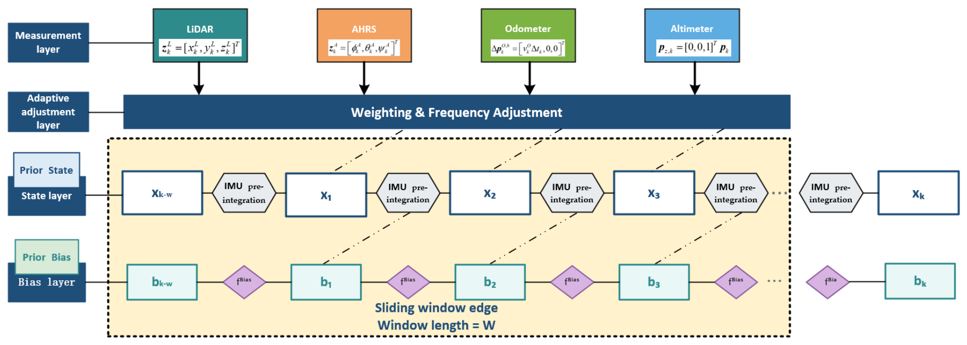
The proposed sliding-window incremental factor graph optimization framework is illustrated in Figure 1. Multi-sensor measurements are inserted as asynchronous factors according to their timestamps, while IMU pre-integration provides high-rate motion propagation between adjacent states. Only variables within the active window are optimized, and historical information is retained through marginalization-derived prior factors.

2.1. System State and Factor Construction

To fuse multi-sensor navigation information in complex motion environments, the carrier navigation state at discrete time k is defined as the state vector of the factor graph optimization system:

$$x_k=[R_k,p_k,v_k,b_{g,k},b_{a,k}]$$

(1)

where ${\mathit{R}}_k\in \mathit{S}\mathit{O}(3)$ denotes the attitude rotation matrix, ${\mathit{p}}_k\in {\mathbb{R}}^3$ denotes the position, ${\mathit{V}}_k\in {\mathbb{R}}^3$ denotes the velocity, and $b_{g,k}\in {\mathbb{R}}^3$ and $b_{a,k}\in {\mathbb{R}}^3$ denotes the gyroscope and accelerometer biases, respectively [12]. The complete state set is denoted by $\mathit{X}=\left\{x_1,x_2,\dots ,x_N\right\}$.

Given the multi-sensor measurement set $\mathit{Z}$, the maximum a posteriori estimate is written as

$${\mathit{X}}^{\ast }=\arg \underset{X}{\max } p(\mathit{X}|\mathit{Z})=\arg \underset{X}{\max } p(\mathit{X})\prod _{i}p({\mathit{z}}_i|\mathit{X}).$$

(2)

Under the Gaussian noise assumption, this estimation problem can be transformed into the following nonlinear least-squares problem:

$$X^{\ast }=\arg \underset{X}{\min }\left\{{\parallel r_0\parallel }_{{\mathsf{\Sigma }}_0^{-1}}^2+\sum _i{\parallel r_i(X)\parallel }_{{\mathsf{\Sigma }}_i^{-1}}^2\right\}$$

(3)

The IMU provides high-rate motion propagation information between adjacent state nodes. Let the measured angular velocity and specific force be denoted by ω and a, respectively. The discrete propagation model is expressed as

$${\mathit{R}}_{k+1}={\mathit{R}}_k\exp \left(({\overline{\mathit{\omega }}}_k-{\mathit{b}}_{g,k}-{\mathit{n}}_{g,k})\Delta t\right)$$

(4)

$${\mathit{v}}_{k+1}={\mathit{v}}_k+\mathit{g}\Delta t+{\mathit{R}}_k({\overline{\mathit{f}}}_{a,k}-{\mathit{b}}_{a,k}-{\mathit{n}}_{a,k})\Delta t$$

(5)

$${\mathit{p}}_{k+1}={\mathit{p}}_k+{\mathit{v}}_k\Delta t+{\displaystyle \frac{1}{2}}\mathit{g}\Delta t^2+{\displaystyle \frac{1}{2}}{\mathit{R}}_k({\overline{\mathit{f}}}_{a,k}-{\mathit{b}}_{a,k}-{\mathit{n}}_{a,k})\Delta t^2$$

(6)

To avoid adding every IMU sample as an individual state node, IMU pre-integration is adopted to compress the high-rate measurements from time i to time j into a single constraint. The corresponding IMU factor residual is

$${\mathit{r}}_{ij}^I={\left[{\mathit{r}}_{\Delta R_{ij}}^T,{\mathit{r}}_{\Delta v_{ij}}^T,{\mathit{r}}_{\Delta p_{ij}}^T,{\mathit{r}}_{b_{g,ij}}^T,{\mathit{r}}_{b_{a,ij}}^T\right]}^T$$

(7)

where

$$\left\{\begin{array}{l}{\mathit{r}}_{\Delta R_{ij}}=\mathrm{Log}\left(\Delta {\mathit{R}}_{ij}^T{\mathit{R}}_i^T{\mathit{R}}_j\right)\\ {\mathit{r}}_{\Delta v_{ij}}={\mathit{R}}_i^T\left({\mathit{v}}_j-{\mathit{v}}_i-\mathit{g}\Delta t_{ij}\right)-\Delta {\mathit{v}}_{ij}\\ {\mathit{r}}_{\Delta p_{ij}}={\mathit{R}}_i^T\left({\mathit{p}}_j-{\mathit{p}}_i-{\mathit{v}}_i\Delta t_{ij}-{\displaystyle \frac{1}{2}}\mathit{g}\Delta t_{ij}^2\right)-\Delta {\mathit{p}}_{ij}\end{array}\right.$$

(8)

2.2. Sensor Factor Construction

To maintain observability of position, velocity, and attitude, asynchronous measurements from LiDAR odometry, the barometer, attitude and heading reference system (AHRS), and wheel odometry (ODO) are fused in a unified factor graph framework. Each sensor measurement is converted into a constraint factor, and the corresponding residual model is constructed according to the physical observation characteristics of the sensor [13].

2.2.1. LiDAR Odometry Position Factor

The LiDAR front end first estimates relative scan-matching increments and then composes these increments into a local LiDAR odometry pose in the initial navigation frame after time synchronization and extrinsic calibration [14]. Therefore, the factor used here should be understood as a local pseudo-position constraint, not as a drift-free global absolute position observation. Let the three-dimensional LiDAR odometry position at time k, expressed in this local navigation frame, be

$${\mathit{z}}_k^L={[x_k^L,y_k^L,z_k^L]}^T$$

(9)

The LiDAR position residual is defined as the difference between the estimated and measured positions:

$${\mathit{r}}_k^L={\mathit{p}}_k-{\mathit{z}}_k^L$$

(10)

The corresponding cost function is

$$J_L=\sum _{k\in \left\{\mathit{L}\right\}}{\left({\mathit{r}}_k^L\right)}^T{\left({\mathsf{\Sigma }}_k^L\right)}^{-1}{\mathit{r}}_k^L$$

(11)

where $\left\{\mathit{L}\right\}$ denotes the set of LiDAR factors, and ${\mathsf{\Sigma }}_k^L$ denotes the covariance matrix propagated from the scan-matching quality, registration degeneracy indicator, and accumulated LiDAR odometry uncertainty. This factor provides local three-dimensional position constraints and suppresses short-term inertial drift, but it does not remove the long-term drift of LiDAR odometry itself. In the reported GNSS-denied experiment, the high-precision SPAN solution is used only for evaluation and is not inserted as an absolute factor.

2.2.2. ODO Velocity Factor

ODO mainly reflects forward motion. Let the forward velocity measured at time k be $v_k^O$, and let the time interval between adjacent state nodes be $\Delta t_k$. The forward displacement is

$$\Delta {\mathit{p}}_k^{O,b}={\left[v_k^O\Delta t_k,0,0\right]}^T$$

(12)

In the body coordinate frame, the corresponding ODO displacement is

$$\Delta {\mathit{p}}_k^{O,n}=R_k\Delta {\mathit{p}}_k^{O,b}$$

(13)

The residual and cost functions of the ODO factor are defined as

$$\left\{\begin{array}{c}{\mathit{r}}_k^O=({\mathit{p}}_{k+1}-{\mathit{p}}_k)-{\mathit{R}}_k{[{\mathit{v}}_k^O\Delta t_k,0,0]}^T\\ {\mathit{J}}_O={\displaystyle \sum _{k\in \left\{\mathit{O}\right\}}}{\left({\mathit{r}}_k^O\right)}^T{\left({\mathsf{\Sigma }}_k^O\right)}^{-1}{\mathit{r}}_k^O\end{array}\right.$$

(14)

where $\left\{\mathit{O}\right\}$ denotes the set of ODO factors and ${\mathsf{\Sigma }}_k^O$ denotes the covariance matrix of the odometry measurement.

2.2.3. Barometer Height Factor

The barometer provides vertical height observations. Let the barometer measurement at time k be $z_k^B$, and let the vertical component of the current position be

$${\mathit{p}}_{z,k}={[0,0,1]}^T{\mathit{p}}_k$$

(15)

The residual and cost function of this factor are defined as

$$\left\{\begin{array}{c}{r}_k^B={\mathit{p}}_{z,k}-z_k^B\\ J_B={\displaystyle \sum _{k\in \left\{\mathit{B}\right\}}}{\displaystyle \frac{{({\mathit{r}}_k^B)}^2}{{\sigma }_{Bk}^2}}\end{array}\right.$$

(16)

where $\left\{\mathit{B}\right\}$ denotes the set of barometer factors and ${\sigma }_{Bk}^2$ denotes the variance of the barometer measurement.

2.2.4. AHRS Attitude Factor

The AHRS outputs roll, pitch, and yaw observations, which are first converted into a unit quaternion using the calibrated body-frame convention. The Euler-angle notation is retained only to describe the sensor output and to report roll, pitch, and yaw errors.

$${\mathit{z}}_k^A={\left[{\varphi }_k^A,{\theta }_k^A,{\psi }_k^A\right]}^T$$

(17)

To avoid the discontinuities caused by directly performing Euler angle subtraction and envelope operations, the pose residual is mapped to a local Lie algebra. The AHRS factor minimizes the Mahalanobis norm of this tangent-space residual:

$$\left\{\begin{array}{c}{\mathit{r}}_{\mathrm{k}}^{\mathrm{A}}=\mathrm{Log}({({\mathit{R}}_{\mathrm{k}}^{\mathrm{A}})}^{\mathrm{T}}{\mathit{R}}_{\mathrm{k}}),\\ {\mathit{J}}_{\mathrm{A}}={\displaystyle \sum _{\mathrm{k}\in \left\{\mathit{A}\right\}}}{({\mathit{r}}_{\mathrm{k}}^{\mathrm{A}})}^{\mathrm{T}}{({\mathsf{\Sigma }}_{\mathrm{k}}^{\mathrm{A}})}^{-1}{\mathit{r}}_{\mathrm{k}}^{\mathrm{A}}\end{array}\right.$$

(18)

Here, $\left\{\mathit{A}\right\}$ denotes the set of AHRS factors, and ${\mathsf{\Sigma }}_k^A$ denotes the covariance matrix of the attitude residual in the local tangent space. This formulation respects the rotation geometry while still allowing component-wise roll, pitch, and yaw covariance inflation in the adaptive weighting stage.

2.3. Sliding-Window and Marginalization Mechanism

Let the sliding-window length be W. The window state set at time k is

$${\mathit{X}}_k^W=\{x_{k-W+1},x_{k-W+2},\dots ,x_k\}$$

(19)

After a new state node $x_{k+1}$ is added, the state set in the updated sliding window becomes

$${\mathit{X}}_{k+1}^W=\{x_{k-W+2},x_{k-W+3},\dots ,x_{k+1}\}$$

(20)

At this point, the earliest state in the window is removed from the active optimization variables [15]. Directly deleting this state and its associated factors would discard historical constraint information. Therefore, a marginalization mechanism is adopted to compress the removed state and its associated factors into a prior factor acting on the retained window states. The marginalized state is defined as

$$x_m=x_{k-W+1}$$

(21)

The retained state is defined as

$$x_r=\{x_{k-W+2},x_{k-W+3},\cdots ,x_{k+1}\}$$

(22)

After the factors associated with the marginalized state $x_{\mathrm{m}}$ are linearized at the current estimate, the following information matrix form is obtained:

$${\displaystyle \frac{1}{2}}{\left[\begin{array}{c}\delta x_m\\ \delta x_r\end{array}\right]}^T\left[\begin{array}{cc}{\mathit{H}}_{mm}& {\mathit{H}}_{mr}\\ {\mathit{H}}_{rm}& {\mathit{H}}_{rr}\end{array}\right]\left[\begin{array}{c}\delta x_m\\ \delta x_r\end{array}\right]-{\left[\begin{array}{c}{\mathit{b}}_m\\ {\mathit{b}}_r\end{array}\right]}^T\left[\begin{array}{c}\delta x_m\\ \delta x_r\end{array}\right]$$

(23)

where $\delta x_m$ is the increment of the marginalized state and $\delta x_r$ is the increment of the retained state. Eliminating $\delta x_m$ using the Schur complement yields the equivalent prior information acting on the retained state:

$$\left\{\begin{array}{c}{\mathit{H}}_p={\mathit{H}}_{rr}-{\mathit{H}}_{rm}{\mathit{H}}_{mm}^{-1}{\mathit{H}}_{mr}\\ {\mathit{b}}_p={\mathit{b}}_r-H_{rm}{H}_{mm}^{-1}{\mathit{b}}_m\end{array}\right.$$

(24)

where ${\mathit{H}}_p$ and ${\mathit{b}}_p$ denote the prior information matrix and prior information vector generated by marginalization, respectively.

In implementation, variables are ordered so that the state to be removed and its directly connected factors are placed in the marginalized block, while the boundary states that remain in the window are placed in the retained block. The associated factors are linearized at the current estimate, the Hessian and gradient are assembled, and the Schur complement is applied to obtain a dense prior on the retained boundary variables. The prior is stored in square-root information form as a linear residual attached to the retained states. To avoid inconsistency from repeatedly relinearizing eliminated information, the Jacobian of the marginalized prior is kept fixed at its marginalization point, while only the active factors inside the current window are relinearized in subsequent incremental updates. As a result, the number of optimized state nodes is bounded by W rather than by the full trajectory length N. If each state has dimension d and the average number of active factors per state is bounded, the dominant local linearization and factorization cost scales with the active window size rather than with N.

The sliding-window optimization objective is therefore written as

$${\mathit{X}}_{k+1}^{W\ast }=\arg \underset{X_{k+1}^W}{\min }\left\{{\mathit{r}}_p{({\mathit{X}}_{k+1}^W)}_{{\mathsf{\Sigma }}_p}^2+\sum _{i\in {\mathcal{I}}_{k+1}^W}{r}_i{({\mathit{X}}_{k+1}^W)}_{{\mathsf{\Sigma }}_i}^2\right\}$$

(25)

where ${\mathit{r}}_p({\mathit{X}}_{k+1}^W)$ denotes the historical prior factor generated by marginalization and ${\mathit{X}}_{k+1}^W$ denotes the set of valid factors in the current window.

This mechanism bounds the number of optimization variables by the window length and prevents continuous growth of the factor graph during long-term operation. States outside the window are no longer optimized explicitly, but their influence on the current window is retained through prior factors, thereby reducing accuracy degradation caused by simply removing historical nodes.

3. Adaptive Optimization Algorithm

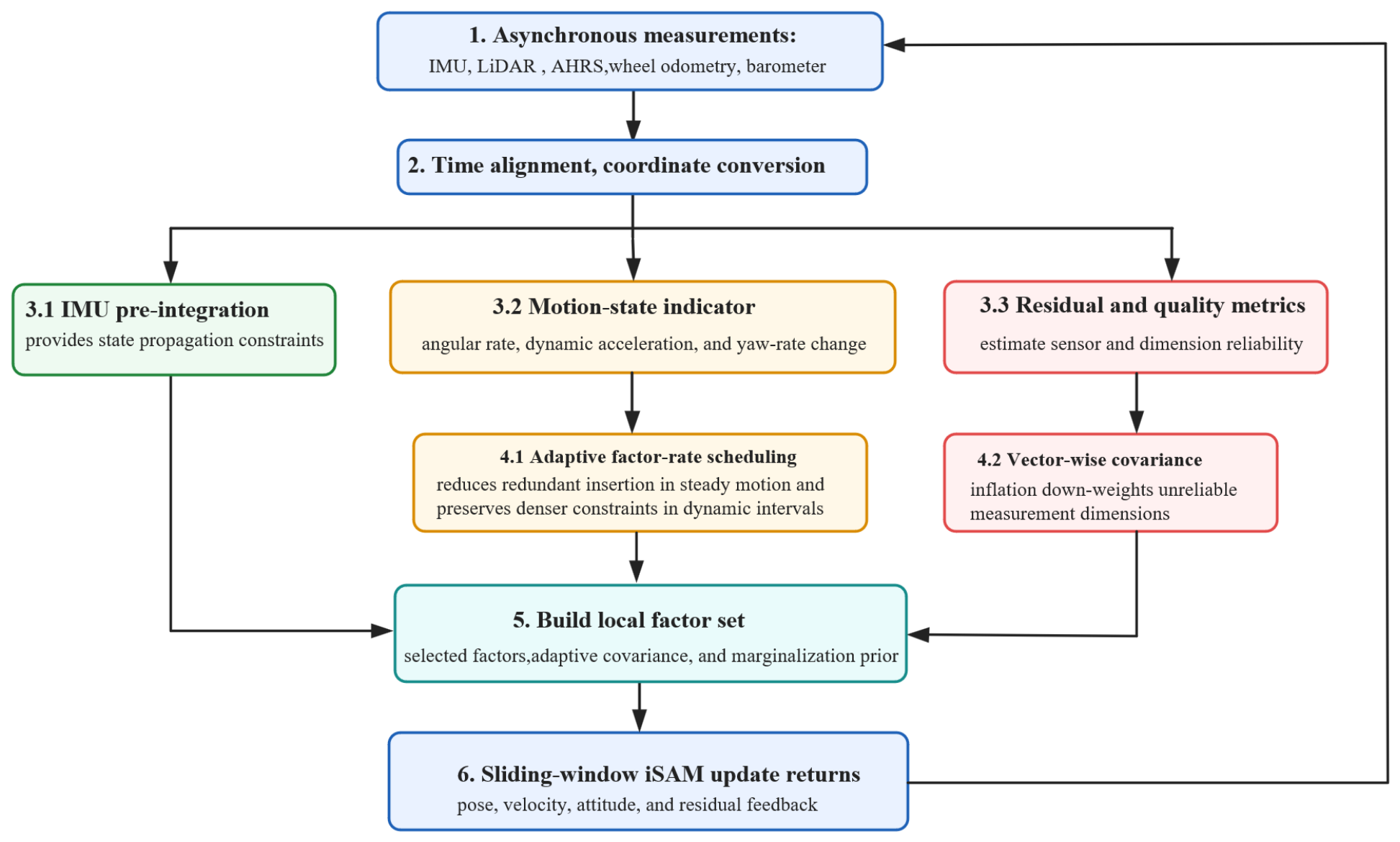
In complex motion environments, the measurement quality of navigation sensors varies over time. If fixed covariance and fixed fusion frequency are used throughout optimization, abnormal measurements may enter the factor graph with unchanged weights and contaminate the state estimate [16]. The factor graph framework is particularly suitable for adaptive processing because each sensor measurement is represented as an independent factor constraint. Factor insertion, removal, weighting, and down-weighting can be performed locally without redefining the system state. Therefore, both the insertion density of sensor factors and the contribution of each measurement dimension can be flexibly controlled. Based on the sliding-window incremental factor graph, this study proposes AVFGO, which jointly incorporates a motion-state-aware adaptive fusion-rate strategy and a residual-driven multi-source adaptive vector-wise weighting factor. The overall workflow of the proposed AVFGO method is shown in Figure 2.

3.1. Adaptive Fusion Rate Based on Motion-State Identification

In complex motion scenarios, a fixed fusion frequency leads to an inherent trade-off between computational efficiency and estimation accuracy [17,18]. Dynamically adjusting the factor insertion rate according to the motion state and environmental conditions can reduce redundant computation during steady motion and increase constraint density during highly dynamic or abnormal intervals. This enables a balance among localization accuracy, robustness, and real-time performance. During straight and low-dynamic driving, frequent insertion of external measurement factors unnecessarily enlarges the optimization graph. In contrast, during sharp turns, acceleration/deceleration, sensor anomalies, or environmental degradation, a higher insertion rate is beneficial for capturing rapid motion changes and limiting short-term error accumulation.

An IMU-assisted motion-state identification mechanism is introduced. First, the deviation between the magnitude of the specific force and gravity is defined as

$$d_{a,k}=|\parallel {\tilde{a}}_k-b_{a,k}\parallel -g|$$

(26)

A large deviation indicates that the accelerometer measurement contains significant non-gravitational acceleration; in this case, the reliability of the AHRS roll and pitch observations should be reduced.

The acceleration deviation and angular-rate indicators are smoothed over a short temporal window before thresholding, so isolated IMU spikes do not immediately switch the fusion-rate state. The thresholds are selected from nominal sensor noise, expected vehicle dynamics, and a short calibration segment, and are reported in the parameter table to make the empirical part of the scheduler explicit.

The magnitude of the angular velocity is defined as

$$d_{\omega ,k}=\parallel {\tilde{\mathit{\omega }}}_k-b_{g,k}\parallel$$

(27)

The yaw rate is calculated from the yaw angles at adjacent epochs as

$${\dot{\psi }}_k={\displaystyle \frac{\mathrm{wrap}\left({\psi }_k-{\psi }_{k-1}\right)}{\Delta t_k}}$$

(28)

Accordingly, the motion-state indicator is calculated as

$$m_k=\left\{\begin{array}{c}0,\hspace{1em}{d}_{a,k}\le {\tau }_a,d_{\omega ,k}\le {\tau }_{\omega },\left|{\dot{\psi }}_k\right|\le {\tau }_{\psi }\hfill \\ 1,\hspace{1em}{d}_{a,k}>{\tau }_a \mathrm{or} d_{\omega ,k}>{\tau }_{\omega } \mathrm{or} \left|{\dot{\psi }}_k\right|>\hfill \end{array}\right.$$

(29)

where $m_k=0$ indicates steady motion, whereas $m_k=1$ indicates turning, highly dynamic motion, or vibration.

The binary motion-state definition is used as a scheduling gate rather than as a complete behavior model of the vehicle. Real vehicle motion is continuous and includes mixed states; however, the factor insertion decision only needs to distinguish intervals in which the nominal low-rate setting is sufficient from intervals that require denser constraints or more conservative weighting. The underlying acceleration, yaw-rate, turn, and residual scores remain continuous and are used in the weighting and rebuild logic. Therefore, the binary label simplifies the scheduler while the covariance inflation and smoothing steps retain graded responses to residual magnitude and IMU dynamics. This threshold-based rule is still limited in highly complex motion environments; probabilistic multiple-model identification, hidden Markov models, or data-driven motion classifiers are more suitable for future cross-platform deployment.

Let the nominal fusion period and nominal fusion frequency of sensor s be $T_0^s$ and $f_0^s$, respectively. At time k, the fusion frequency $f_k^s$ is adjusted according to the motion state $m_k$, measurement residual $e_k^s$, and quality indicator $q_k^s$ as

$$f_k^s=f_0^s{\rho }_k^s$$

(30)

where ${\rho }_k^s$ is the fusion-rate adjustment coefficient. A smaller value is used in steady motion, whereas ${\rho }_k^s$ is increased during turning, highly dynamic motion, or abnormal measurements to increase the density of key constraints and improve the observability of adaptive weighting.

The coefficient is a resource-allocation rule for factor insertion rather than a posterior probability of a motion class. It is designed to be monotonic with respect to normalized residual and motion-intensity scores, bounded by preset minimum and maximum insertion rates, and smoothed between adjacent epochs. Consequently, the rule avoids unbounded graph growth and prevents rapid oscillation of the sensor update interval, but its numerical thresholds remain empirical and dataset dependent.

The fusion-rate adjustment coefficient is defined as

$${\rho }_k^s=1+c_m^s{m}_k+c_r^s\max \left(0,{\displaystyle \frac{e_k^s-{\tau }_r^s}{{\tau }_r^s}}\right)+c_q^s\max \left(0,{\displaystyle \frac{{\tau }_q^s-q_k^s}{{\tau }_q^s}}\right)$$

(31)

The upper and lower bounds are set as

$$\left\{\begin{array}{c}{\rho }_{\min }^s\le {\rho }_k^s\le {\rho }_{\max }^s\\ f_{\min }^s\le f_k^s\le f_{\max }^s\end{array}\right.$$

(32)

In implementation, the fusion frequency is controlled through the factor insertion interval. If the nominal insertion interval is $N_0^s$, the adaptive insertion interval is

$$N_k^s={\displaystyle \frac{N_0^s}{{\rho }_k^s}},N_{\min }^s\le N_k^s\le N_{\max }^s$$

(33)

Typical rules for adaptive fusion frequency are as follows:

$$\left\{\begin{array}{c}\left|{\dot{\psi }}_k\right|>{\tau }_{\dot{\psi }}\Rightarrow {\rho }_k^A\uparrow ,\hspace{1em}{\rho }_k^L\uparrow \\ m_k=0\Rightarrow {\rho }_k^s\downarrow \\ e_k^L>{\tau }_L\Rightarrow {\rho }_k^A\uparrow ,\hspace{1em}{\rho }_k^O\uparrow ,\hspace{1em}{\gamma }_k^L\uparrow \end{array}\right.$$

(34)

Here, increasing ${\gamma }_k^L$ reduces the weight of abnormal LiDAR factors, whereas increasing ${\rho }_k^A$ and ${\rho }_k^O$ enhances the density of attitude and motion constraints. This strategy prevents abnormal sensors from continuously biasing the estimate through high-rate measurements while preserving necessary constraints during critical motion intervals.

3.2. Residual-Driven Adaptive Weighting Factor

In practical complex environments, however, sensor reliability varies with environmental structure, vehicle motion, and measurement dimension. If fixed covariance parameters are used, abnormal measurements may contaminate the optimization process. Therefore, a multi-source adaptive vector-wise weighting factor is proposed to independently regulate the contributions of different sensors and measurement dimensions. The model is mathematically equivalent to a bounded iteratively reweighted least-squares layer: at each outer update, the current residuals and motion-quality indicators define positive covariance-inflation coefficients; with these coefficients fixed, the inner problem remains a standard Gaussian nonlinear least-squares problem.

Let the nominal covariance of sensor s at time k be ${\mathsf{\Sigma }}_{k,0}^s$, where $S\in \left\{\mathit{L},\mathit{O},\mathit{B},\mathit{A}\right\}$ denotes LiDAR, ODO, barometer, or AHRS. The adaptive adjustment matrix is constructed as

$${\mathsf{\Gamma }}_k^s=\mathrm{diag}\left({\gamma }_{k,1}^s,{\gamma }_{k,2}^s,\dots ,{\gamma }_{k,n_s}^s\right)$$

(35)

where n_s is the measurement dimension of sensor s and ${\gamma }_{k,j}^s$ is the adaptive adjustment coefficient of the j-th measurement dimension.

The effective covariance is then

$${\mathsf{\Sigma }}_{k,\mathrm{eff}}^s={\mathsf{\Gamma }}_k^s{\mathsf{\Sigma }}_{k,0}^s{\mathsf{\Gamma }}_k^s$$

(36)

Since factor weight is inversely proportional to covariance, increasing ${\gamma }_{k,j}^s$ increases the covariance of the corresponding dimension and decreases its factor weight. To avoid erroneously enhancing abnormal measurements, ${\gamma }_{k,j}^s$ is constrained as follows:

$$1\le {\gamma }_{k,j}^s\le {\gamma }_{\max }^s$$

(37)

For each measurement dimension, the normalized residual metric is explicitly computed from the actual factor residual before updating the adaptive coefficient:

$${\eta }_{k,j}^s={\displaystyle \frac{\left|{\gamma }_{k,j}^s\right|}{{\sigma }_{0,j}^s+\epsilon }}$$

(38)

$${\gamma }_{k,j}^s=\left\{\begin{array}{cc}1& {\eta }_{k,j}^s\le {\tau }_1^s\\ 1+{\alpha }^s\left({\eta }_{k,j}^s-{\tau }_1^s\right)& {\tau }_1^s<{\eta }_{k,j}^s\le {\tau }_2^s\\ {\gamma }_{\max }^s& {\eta }_{k,j}^s>{\tau }_2^s\end{array}\right.$$

(39)

where ${\tau }_1^s$ is the normal threshold, ${\tau }_2^s$ is the anomaly threshold, and ${\alpha }^s$ is the adjustment slope.

$${\overline{\gamma }}_{k,j}^s=\lambda {\overline{\gamma }}_{k-1,j}^s+(1-\lambda ){\gamma }_{k,j}^s,\hspace{1em}\lambda \in [0,1)$$

(40)

3.2.1. LiDAR Position Adaptive Weighting Factor

The basic covariance is

$${\mathsf{\Gamma }}_k^L=\mathrm{diag}\left({\gamma }_{x,k}^L,{\gamma }_{y,k}^L,{\gamma }_{z,k}^L\right)$$

(41)

The effective covariance is

$${\mathsf{\Sigma }}_{k,\mathrm{eff}}^L=\mathrm{diag}\left({({\gamma }_{x,k}^L{\sigma }_{x,L})}^2,{({\gamma }_{y,k}^L{\sigma }_{y,L})}^2,{({\gamma }_{z,k}^L{\sigma }_{z,L})}^2\right)$$

(42)

The horizontal and vertical LiDAR residuals are defined as

$$\left\{\begin{array}{c}{e}_{xy,k}^L=\sqrt{{\left({\gamma }_{x,k}^L\right)}^2+{\left({\gamma }_{y,k}^L\right)}^2}\\ e_{z,k}^L=\left|\begin{array}{c}{\gamma }_{z,k}^L\end{array}\right|\end{array}\right.$$

(43)

Considering both the residual and the motion state $m_k$, the horizontal adjustment coefficient is written as

$${\gamma }_{xy,k}^L=1+{\alpha }_L\max \left(0,{\displaystyle \frac{e_{xy,k}^L-{\tau }_{xy}^L}{{\tau }_{xy}^L}}\right)+{\beta }_L{m}_k$$

(44)

The adjustment factors are

$$\left\{\begin{array}{c}{\gamma }_{x,k}^L=\min \left({\gamma }_{xy,k}^L,{\gamma }_{\max }^L\right)\\ {\gamma }_{y,k}^L=\min \left({\gamma }_{xy,k}^L,{\gamma }_{\max }^L\right)\\ {\gamma }_{z,k}^L=\min \left[1+{\alpha }_{z,L}\max \left(0,{\displaystyle \frac{e_{z,k}^L-{\tau }_z^L}{{\tau }_z^L}}\right),{\gamma }_{\max }^L\right]\end{array}\right.$$

(45)

3.2.2. AHRS Attitude Adaptive Weighting Factor

The basic covariance is

$${\mathsf{\Gamma }}_k^A=\mathrm{diag}\left({\gamma }_{\varphi ,k}^A,{\gamma }_{\theta ,k}^A,{\gamma }_{\psi ,k}^A\right)$$

(46)

The corresponding effective covariance is

$${\mathsf{\Sigma }}_{k,\mathrm{eff}}^A=\mathrm{diag}\left[{\left({\gamma }_{\varphi ,k}^A{\sigma }_{\varphi ,A}\right)}^2,{\left({\gamma }_{\theta ,k}^A{\sigma }_{\theta ,A}\right)}^2,{\left({\gamma }_{\psi ,k}^A{\sigma }_{\psi ,A}\right)}^2\right]$$

(47)

Roll and pitch are sensitive to non-gravitational acceleration; therefore, their weighting coefficients are adjusted using the specific-force magnitude deviation:

$$\left\{\begin{array}{c}{\gamma }_{\varphi ,k}^A=\min \left[1+{\alpha }_{\varphi ,A}\max \left(0,{\displaystyle \frac{{\Delta }_{a,k}-{\tau }_a}{{\tau }_a}}\right),{\gamma }_{\max }^A\right]\\ {\gamma }_{\theta ,k}^A=\min \left[1+{\alpha }_{\theta ,A}\max \left(0,{\displaystyle \frac{{\Delta }_{a,k}-{\tau }_a}{{\tau }_a}}\right),{\gamma }_{\max }^A\right]\end{array}\right.$$

(48)

The yaw adjustment coefficient considers both yaw residual and yaw rate:

$${\gamma }_{\psi ,k}^A=\min \left[1+{\alpha }_{\psi ,A}\max \left(0,{\displaystyle \frac{\left|r_{\psi ,k}^A\right|-{\tau }_{\psi }^A}{{\tau }_{\psi }^A}}\right)+{\beta }_{\psi ,A}\max \left(0,{\displaystyle \frac{\left|{\dot{\psi }}_k\right|-{\tau }_{\psi }}{{\tau }_{\psi }}}\right),{\gamma }_{\max }^A\right]$$

(49)

3.2.3. ODO Velocity Adaptive Weighting Factor

Because ODO provides a strong constraint in the forward direction but only weak constraints laterally and vertically, the nominal covariance is set as

$${\mathsf{\Sigma }}_{k,0}^O=\mathrm{diag}({\sigma }_{f,O}^2,{\sigma }_{l,O}^2,{\sigma }_{u,O}^2)$$

(50)

The forward adjustment factor is

$${\gamma }_{f,k}^O=\min \left[1+{\alpha }_O\max \left(0,{\displaystyle \frac{\left|\begin{array}{c}{v}_k^O-{\mathit{e}}_x^T{\mathit{R}}_k^T{\mathit{v}}_k\end{array}\right|-{\tau }_v^O}{{\tau }_v^O}}\right)+{\beta }_O\max \left(0,{\displaystyle \frac{|v_k^O-v_{k-1}^O|-{\tau }_{\Delta v}^O}{{\tau }_{\Delta v}^O}}\right),{\gamma }_{\max }^O\right]$$

(51)

The lateral and vertical directions are treated as weak fixed constraints:

$$\left\{\begin{array}{c}{\gamma }_{l,k}^O={\gamma }_{l,0}^O>1\\ {\gamma }_{u,k}^O={\gamma }_{u,0}^O>1\end{array}\right.$$

(52)

3.2.4. Barometer Vertical Adaptive Weighting Factor

For the barometer height factor, the height jump $d_{h,k}^B$ and vertical consistency error $e_{h,k}^B$ are defined as

$$\left\{\begin{array}{c}{d}_{h,k}^B=\left|\begin{array}{c}{z}_k^B-z_{k-1}^B\end{array}\right|\\ e_{h,k}^B=\left|\begin{array}{c}{p}_{z,k}-z_k^B\end{array}\right|\end{array}\right.$$

(53)

The effective barometer variance is then

$${\sigma }_{B,k,\mathrm{eff}}^2={\left({\gamma }_k^B{\sigma }_{B,0}\right)}^2$$

(54)

where

$${\gamma }_k^B=\min \left[1+{\alpha }_B\max \left(0,{\displaystyle \frac{e_{h,k}^B-{\tau }_h^B}{{\tau }_h^B}}\right)+{\beta }_B\max \left(0,{\displaystyle \frac{d_{h,k}^B-{\tau }_{\Delta h}^B}{{\tau }_{\Delta h}^B}}\right),{\gamma }_{\max }^B\right]$$

(55)

Together, these models constitute the proposed adaptive vector-wise factor.

4. Experimental Validation

4.1. Experimental Setup

To verify the effectiveness of the proposed method, field experiments were conducted using a ground wheeled unmanned vehicle platform under a GNSS-denied evaluation setting. The analysis focuses on four aspects: (1) comparing AVFGO with full incremental and fixed sliding-window factor graphs; (2) isolating the effects of sliding-window optimization, scalar adaptive weighting, and vector-wise adaptive weighting; (3) reporting parameter values and runtime-complexity indicators; and (4) discussing the limitations caused by using one outdoor trajectory from one platform. The experiment therefore supports method-level validation on the collected dataset, while cross-platform and cross-scene generalization remain future work.

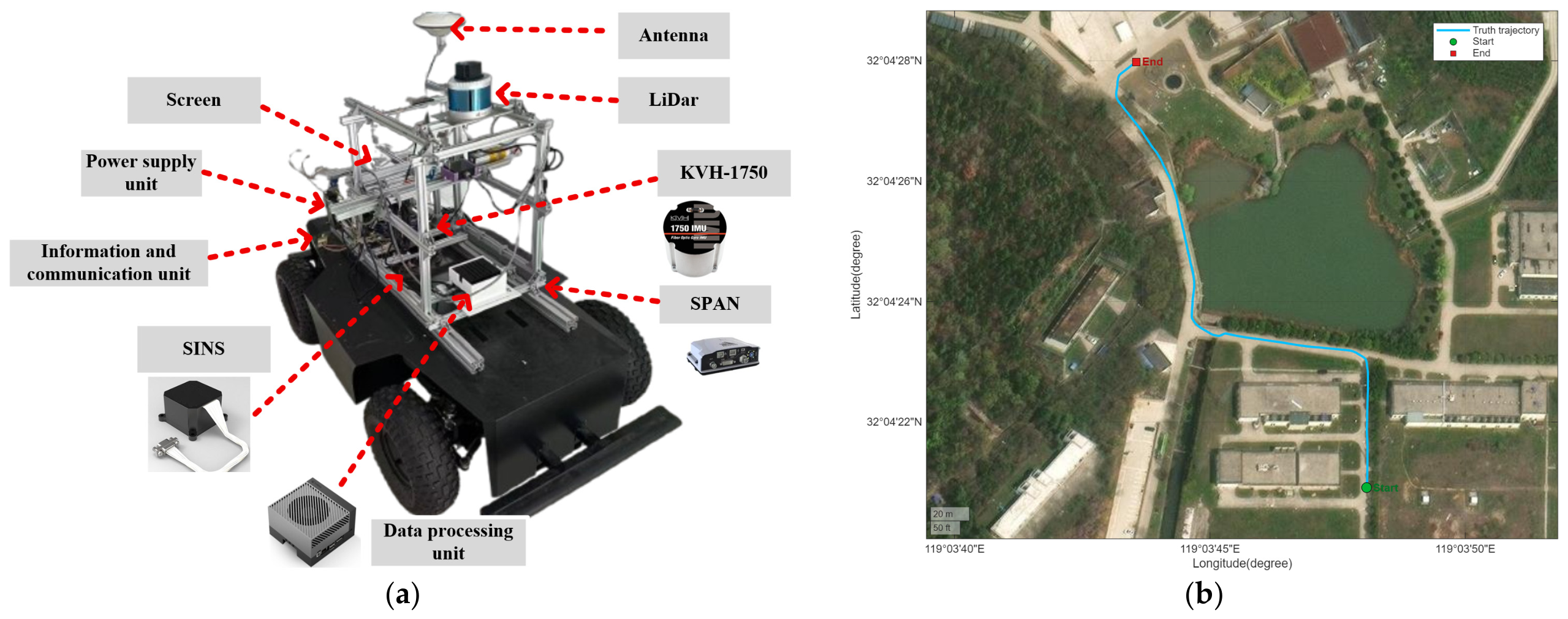
The experimental platform is shown in Figure 3. It is equipped with an NVIDIA Jetson AGX ORIN computing unit, a STIM300 IMU, a C16 LiDAR, an AHRS, wheel odometry, and a barometer as the core navigation sensors. A NovAtel SPAN-KVH1750 integrated navigation system is used only as the high-precision reference for error evaluation, and GNSS measurements are not inserted into the factor graph during the reported no-GNSS experiment. Sensor data acquisition, preprocessing, and the fusion algorithm are deployed under Ubuntu 20.04 with ROS Noetic. The main sensor parameters are listed in

Table 1. Sensor parameters.

Device		Parameter		Value
IMU	Gyroscope	Bias stability		≤5°/h
	Accelerometer			≤0.25 mg
C16 LiDAR		Distance measurement accuracy		±3 cm
Wheel odometry		Velocity accuracy (RMSE)		0.05 m/s
Barometer		Altitude measurement accuracy		±15 cm
AHRS		Magnetic field resolution		0.1 nT
SPAN-KVH1750		Position accuracy (RMSE)	Horizontal	0.15 m
			Vertical	0.09 m
		Velocity accuracy (RMSE)	Horizontal	0.02 m/s
			Vertical	0.01 m/s
		Attitude accuracy (RMSE)	Heading angle	0.035°
			Pitch angle, roll angle	0.015°

. IMU measurements are timestamped using a chip-level hardware clock to reduce integration errors caused by unstable host timestamps. The trajectory includes straight driving, turning, acceleration/deceleration, and local environmental variations, making it suitable for evaluating motion-state-aware fusion on this platform.

Thresholds were initialized from nominal sensor specifications and then adjusted on a short training segment to avoid excessive covariance inflation during steady motion. The residual thresholds are deliberately separated into normal and abnormal regions so that small residuals keep the nominal covariance, medium residuals produce gradual inflation, and large residuals reach a bounded maximum. The parameters are therefore empirical design values, not universal constants; their role is documented to improve reproducibility, and sensitivity results are reported to show how the method behaves when representative thresholds are changed. The main numerical parameters used in the final AVFGO implementation are summarized in

Table 2. Main parameter settings used in AVFGO.

Device	Parameter	Value
LiDAR factor	Residual threshold	[0.5, 0.5, 0.8] m/[2, 2, 3] m
	Adaptive gain upper bound	[6, 6, 10] (dimensionless)
AHRS factor	Residual threshold	[1, 1, 2] deg/[5, 5, 15] deg
	Adaptive gain upper bound	[6, 6, 20] (dimensionless)
Barometer factor	Residual threshold	0.30 m/1.5 m
	Adaptive gain upper bound	10 (dimensionless)
ODO factor	Forward velocity variance	0.08 (m/s)2
	Lateral/vertical variance	1.20 (m/s)2

.

4.2. Experimental Analysis

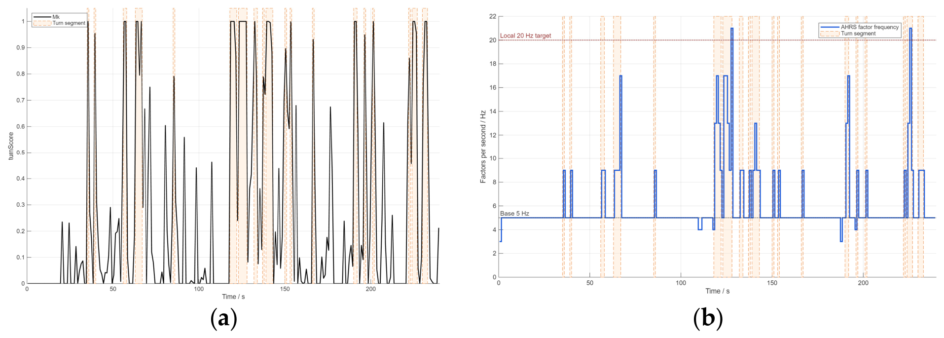
To evaluate the effectiveness of the proposed improvements, AVFGO is compared with fixed-covariance FGO, incremental full factor graph optimization (IFGO), fixed sliding-window factor graph optimization (SWIFGO), and a scalar adaptive weighting variant. Figure 4 shows the IMU-based motion-state identification and sensor frequency modulation. During steady straight motion, redundant external-factor insertion is reduced or kept at the nominal low-rate setting. During rapid-turn intervals, attitude and motion constraints are retained more densely, allowing the estimator to respond to short-term dynamics without allowing the graph size to grow unbounded.

The baseline set is intended to isolate the effects of full-graph accumulation, fixed sliding-window optimization, scalar adaptive weighting, and vector-wise adaptive weighting under the same sensor configuration. It does not constitute a complete comparison against all robust FGO strategies. Robust kernels, dynamic covariance scaling, and switchable constraints can also suppress abnormal factors, and a sensor-matched implementation of these alternatives is left as future work.

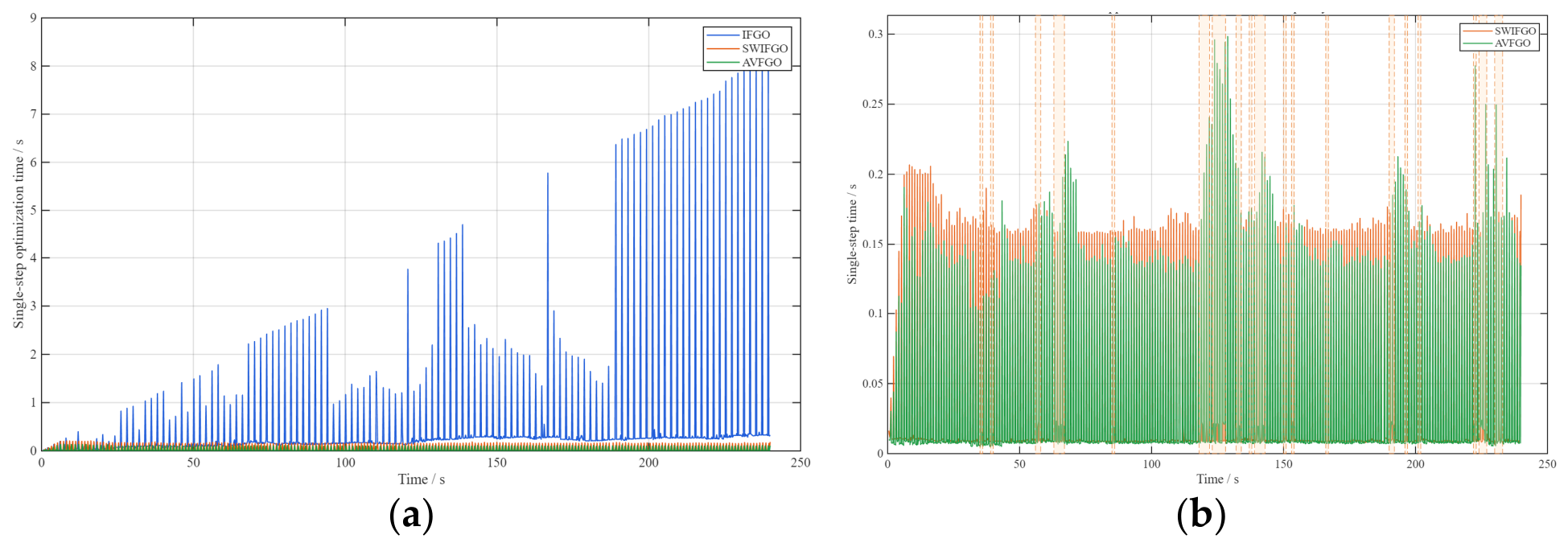
Figure 5 compares the optimization time of the algorithms. Because IFGO continuously accumulates historical states, its single-step optimization time increases with operation time, and the maximum single-step time reaches 8.18 s in the 240 s no-GNSS experiment. SWIFGO bounds the state size using a fixed window and reduces the mean time to 0.16 s. AVFGO further reduces the mean time to 0.04 s by combining bounded-window optimization with adaptive factor management. The runtime difference between AVFGO and the scalar adaptive sliding-window variant is small, so the main claim is not that vector-wise weighting alone greatly accelerates the optimizer. Instead, AVFGO maintains essentially the same real-time cost as the adaptive sliding-window variant while providing a much larger accuracy improvement. During the 61 high-dynamic samples identified by the scheduler, the AVFGO mean time increases from 0.04 s to 0.06 s, indicating that extra computation is allocated to critical motion intervals while real-time performance is preserved.

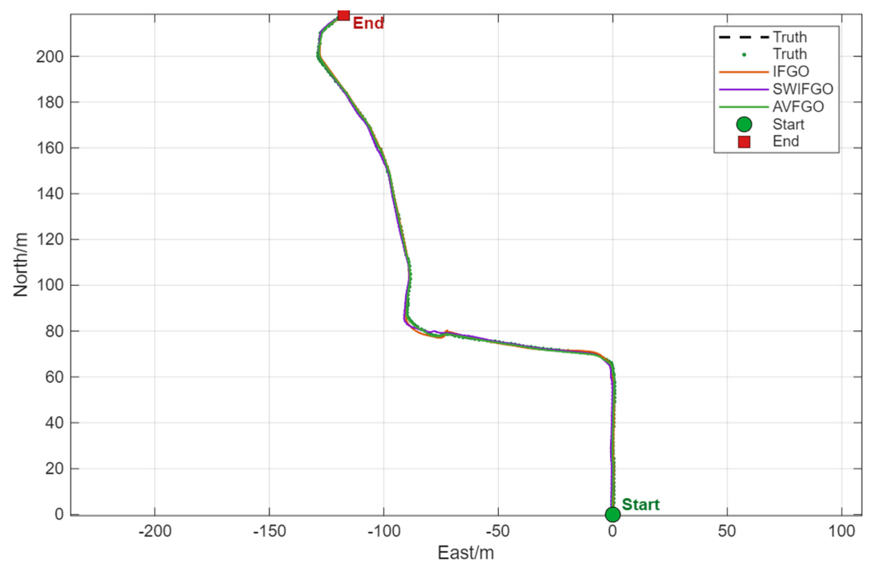
Figure 6 compares the trajectories obtained by the three methods. All methods continuously track the reference trajectory, but their errors differ in turning and locally degraded regions. The root mean square error (RMSE) over the complete experiment is used to evaluate navigation accuracy. The positioning error at time k and the overall RMSE are defined as follows

$$e_{p,k}=\sqrt{{(p_{E,k}-p_{E,k}^{\mathrm{ref}})}^2+{(p_{N,k}-p_{N,k}^{\mathrm{ref}})}^2+{(p_{U,k}-p_{U,k}^{\mathrm{ref}})}^2}$$

(56)

$$RMS{E}_p=\sqrt{{\displaystyle \frac{1}{N}}{\displaystyle \sum _{k=1}^N}{e}_{p,k}^2}$$

(57)

where $(p_{E,k},p_{N,k},p_{U,k})$ denote the estimated east, north, and up positions, respectively, and $(p_{E,k}^{ref},p_{N,k}^{ref},p_{U,k}^{ref})$ denotes the reference values provided by the ground-truth system. Attitude and velocity errors are evaluated in the same manner.

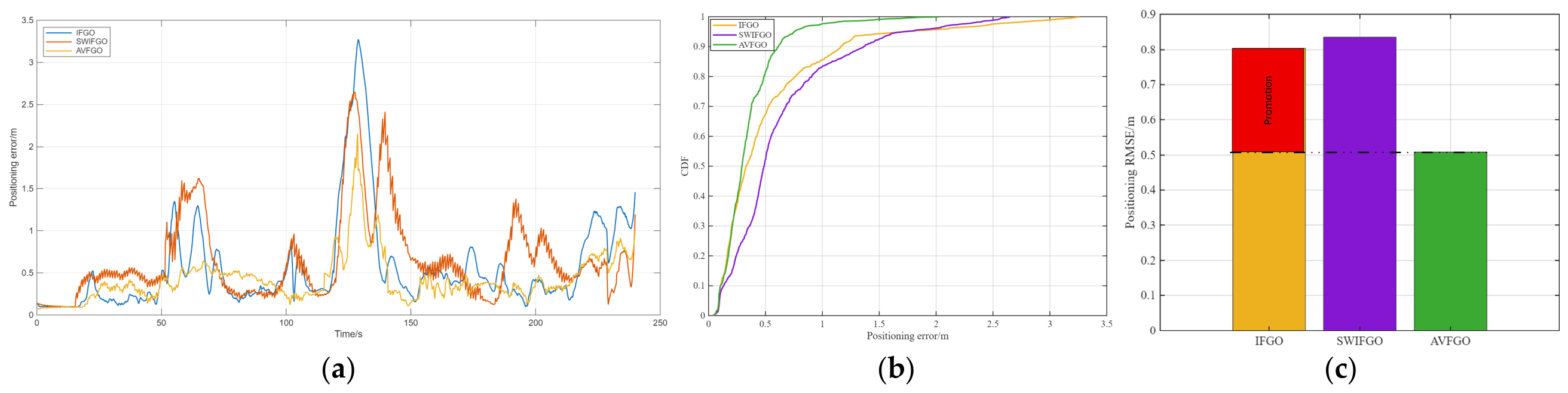
Figure 7 shows the horizontal positioning error over time. During steady driving, all methods remain bounded, whereas errors increase in turning and locally degraded intervals. AVFGO produces lower error peaks and faster recovery because the vector-wise adaptive weighting factor suppresses unreliable measurement dimensions instead of applying a single scalar weight to the whole sensor factor. The 3D position RMSE is reduced from 1.098 m for IFGO and 0.804 m for SWIFGO to 0.380 m for AVFGO, corresponding to reductions of 65.36% and 52.71%, respectively.

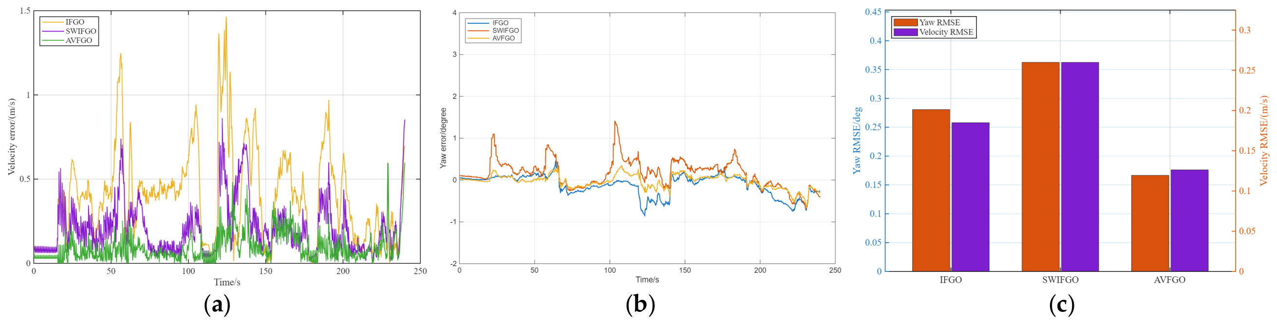
Figure 8 shows the velocity and yaw error comparison, and

Table 3. Performance comparison of different methods in the 240 s no-GNSS experiment.

Method	Position RMSE (m)	Yaw RMSE (Deg)	Mean Time (s)
Fixed covariance	1.098	0.281	0.4650
IFGO	1.098	0.281	0.4629
SWIFGO	0.804	0.691	0.1609
Scalar adaptive	0.890	0.521	0.0402
AVFGO	0.380	0.167	0.0389

summarizes the quantitative performance of the five tested variants. The scalar adaptive variant improves attitude accuracy relative to SWIFGO but does not consistently improve 3D position RMSE, showing that a single sensor-level scale factor is insufficient for heterogeneous measurement dimensions. AVFGO achieves the best overall position, roll, pitch, yaw, and computation-time balance in this dataset. The table also makes clear that the reported gain comes mainly from the combined sliding-window and vector-wise adaptive model in accuracy and robustness, whereas the computational gain over another bounded adaptive variant is marginal.

Overall, AVFGO improves the error distribution and stability of localization results in the collected complex-motion dataset. Table 3 isolates the contribution of adaptive weighting,

Table 4. Ablation study of adaptive weighting.

Variant	Position RMSE (m)	Yaw RMSE (Deg)	Interpretation
No adaptive weighting (SW fixed)	0.804	0.691	No vector-wise covariance adaptation
Scalar adaptive weighting	0.890	0.521	Sensor-level scaling improves attitude but not position
Vector adaptive weighting (proposed clean)	0.380	0.167	Dimension-wise scaling gives the best overall balance

reports the runtime-complexity evidence used to support the real-time claim,

Table 5. Runtime and bounded-window statistics.

Method	Mean Time (s)	Max Time (s)	Total Time (s)	Speedup vs. IFGO
IFGO	0.4629	8.177	551.74	1.00×
SWIFGO	0.1609	0.215	191.85	2.88×
AVFGO	0.0389	0.198	46.41	11.89×

provides diagnostic sensitivity and stress-test results, and

Table 6. Scope comparison with representative external baselines.

Method Family	Typical Focus	Relation to AVFGO	Comparison Status
VINS-Mono/visual-inertial FGO	Camera-IMU smoothing with visual feature tracking and loop handling	Shares IMU pre-integration and factor-graph smoothing but requires visual front-end measurements not used in the vehicle dataset	Discussed as related work; not a sensor-matched experimental baseline
LIO-SAM/LiDAR-inertial SLAM	LiDAR feature odometry, IMU pre-integration, local mapping, and optional loop/global constraints	Closest public factor-graph family, but primarily a SLAM mapping system rather than the LiDAR/AHRS/ODO/barometer fusion problem studied here	Discussed as related work; future direct comparison requires matched front-end configuration
FAST-LIO2/direct LiDAR-inertial odometry	High-rate direct LiDAR-inertial estimation and mapping	Provides strong real-time LiDAR-inertial baseline but does not evaluate AHRS, ODO, or barometer vector-wise adaptive weighting	Discussed as related work; no direct accuracy claim is made
Robust-kernel/switchable-constraint FGO	Outlier-robust residual weighting, dynamic covariance scaling, or latent switch variables for abnormal factors	Closest robust-estimation family to the residual-consistency idea; AVFGO differs by combining bounded vector-wise covariance inflation with motion-state factor-rate scheduling	Conceptual comparison added; a sensor-matched robust-kernel or switchable-constraint experiment is future work
AVFGO (this work)	Bounded-window multi-sensor fusion with motion-state scheduling and vector-wise covariance inflation	Targets GNSS-denied unmanned ground vehicle localization using IMU, LiDAR odometry, AHRS, ODO, and barometer	Experimentally evaluated on the reported 240 s vehicle dataset

clarifies how AVFGO differs from representative external baselines. The results show that sliding-window optimization controls graph growth, vector-wise adaptive weighting provides the largest accuracy improvement, and the bounded active window keeps the mean optimization time below the state-update period used in the experiment.

Segmented timing further shows that AVFGO uses 0.0373 s per step in non-increased-frequency intervals and 0.0555 s per step during the detected high-dynamic intervals. Thus, the scheduler increases computation only when additional constraints are useful, while the sliding window prevents long-term graph growth.

4.3. Diagnostic Sensitivity and External Baseline Positioning

To respond to the concern that the adaptive rules contain heuristic thresholds, additional diagnostic tests were organized from the existing experimental outputs. These tests are not presented as exhaustive parameter optimization; rather, they illustrate the sensitivity of the system to representative frequency, observability, and attitude-parameter changes. The results in Table 6 show that the nominal setting gives the best balance in the tested trajectory, while overly aggressive AHRS/ODO high-rate insertion or excessive LiDAR down-sampling can degrade position accuracy.

Directly rerunning every public baseline on the same sensor configuration was not feasible because several representative systems require different sensor suites, front-end maps, or loop-closure modules. In addition, robust-kernel FGO, dynamic covariance scaling, and switchable-constraint formulations require dedicated residual models and tuning for the same LiDAR/AHRS/ODO/barometer factor set [17,18]. Therefore, Table 6 is added as a scope comparison rather than an accuracy ranking. It clarifies that AVFGO is intended for bounded-window, GNSS-denied, heterogeneous vehicle-sensor fusion, while public SLAM baselines emphasize visual-inertial or LiDAR-inertial mapping pipelines. The current experiments show that AVFGO improves over fixed-covariance and scalar-adaptive variants in the reported dataset, but they do not prove superiority over all robust FGO methods.

5. Conclusions

This study proposes AVFGO, a sliding-window incremental factor-graph-based adaptive multi-sensor fusion localization method for complex motion environments. The revised manuscript clarifies that the main novelty of AVFGO lies in the integration of motion-state-aware factor scheduling and residual-driven vector-wise adaptive weighting within a bounded sliding-window factor graph, rather than in the introduction of a new factor-graph estimation principle. In the 240 s GNSS-denied field experiment, AVFGO achieves a 3D position RMSE of 0.380 m and a mean single-step optimization time of 0.0389 s, outperforming IFGO and SWIFGO in both localization accuracy and runtime on the tested platform.

Several limitations remain to be addressed in future work. The current validation is based on a single outdoor trajectory and a single wheeled platform, which limits the generalizability of the results. Therefore, repeated trials, cross-platform experiments using heterogeneous robotic systems, and cross-scene validation will be conducted to quantify statistical variability, robustness, and adaptability. In addition, controlled degradation tests involving packet loss, communication delay, sensor bias injection, abnormal measurements, and nonlinear disturbances will be introduced to further evaluate the resilience of AVFGO under challenging real-world conditions. Methodologically, the current motion-state identification rule and bounded covariance-inflation strategy will be further improved, potentially through probabilistic or learning-based motion-mode recognition and more comprehensive robust weighting models.

References

1. Qu, Y.; Yang, M.; Zhang, J.; Xie, W.; Qiang, B.; Chen, J. An Outline of Multi-Sensor Fusion Methods for Mobile Agents Indoor Navigation. Sensors 2021, 21, 1605. [Google Scholar] [CrossRef] [PubMed]
2. Wen, W.; Pfeifer, T.; Bai, X.; Hsu, L. Factor Graph Optimization for GNSS/INS Integration: A Comparison with the Extended Kalman Filter. Navig. J. Inst. Navig. 2021, 68, 315–331. [Google Scholar] [CrossRef]
3. Knight, N.; Wang, J. A Comparison of Outlier Detection Procedures and Robust Estimation Methods in GPS Positioning. J. Navig. 2009, 62, 699–709. [Google Scholar] [CrossRef]
4. Kaess, M.; Johannsson, H.; Roberts, R.; Ila, V.; Leonard, J.J.; Dellaert, F. ISAM2: Incremental Smoothing and Mapping Using the Bayes Tree. Int. J. Robot. Res. 2012, 31, 216–235. [Google Scholar]
5. Lynen, S.; Achtelik, M.W.; Weiss, S.; Chli, M.; Siegwart, R. A Robust and Modular Multi-Sensor Fusion Approach Applied to MAV Navigation. In 2013 IEEE/RSJ International Conference on Intelligent Robots and Systems; IEEE: Piscataway, NJ, USA, 2013; pp. 3923–3929. [Google Scholar]
6. Dellaert, F.; Kaess, M. Factor Graphs for Robot Perception. Found. Trends Robot. 2017, 6, 1–139. [Google Scholar] [CrossRef]
7. Wen, W.; Hsu, L.T. Towards Robust GNSS Positioning and Real-Time Kinematic Using Factor Graph Optimization. In 2021 IEEE International Conference on Robotics and Automation (ICRA); IEEE: Piscataway, NJ, USA, 2021; pp. 5884–5890. [Google Scholar]
8. Shan, T.; Englot, B.; Meyers, D.; Wang, W.; Ratti, C.; Rus, D. LIO-SAM: Tightly-Coupled Lidar Inertial Odometry via Smoothing and Mapping. In 2020 IEEE/RSJ International Conference on Intelligent Robots and Systems (IROS); IEEE: Piscataway, NJ, USA, 2020; pp. 5135–5142. [Google Scholar]
9. Xu, W.; Cai, Y.; He, D.; Lin, J.; Zhang, F. FAST-LIO2: Fast Direct LiDAR-Inertial Odometry. IEEE Trans. Robot. 2022, 38, 2053–2073. [Google Scholar] [CrossRef]
10. Zhang, J.; Singh, S. LOAM: Lidar Odometry and Mapping in Real-Time. In Robotics: Science and Systems; MIT Press: Cambridge, MA, USA, 2014. [Google Scholar]
11. Bai, X.; Wen, W.; Hsu, L.T. Time-Correlated Window Carrier-Phase-Aided GNSS Positioning Using Factor Graph Optimization for Urban Positioning. IEEE Trans. Aerosp. Electron. Syst. 2022, 58, 3370–3384. [Google Scholar] [CrossRef]
12. Qin, T.; Li, P.; Shen, S. VINS-Mono: A Robust and Versatile Monocular Visual-Inertial State Estimator. IEEE Trans. Robot. 2018, 34, 1004–1020. [Google Scholar] [CrossRef]
13. Dellaert, F. Factor Graphs and GTSAM: A Hands-On Introduction; Georgia Institute of Technology Technical Report; Georgia Institute of Technology: Atlanta, GA, USA, 2012. [Google Scholar]
14. Hu, P.; Chen, Y.; Jiang, C.; Lin, Q.; Li, W.; Qi, J.; Yu, L.; Hui Shao, H. Spectral observation and classification of typical tree species leaves based on indoor hyperspectral lidar. J. Infrared Millim. Waves 2020, 39, 372–380. [Google Scholar]
15. Olson, E.; Agarwal, P. Inference on Networks of Mixtures for Robust Robot Mapping. Int. J. Robot. Res. 2013, 32, 826–840. [Google Scholar] [CrossRef]
16. Li, X.R.; Jilkov, V.P. Survey of Maneuvering Target Tracking. Part V: Multiple-Model Methods. IEEE Trans. Aerosp. Electron. Syst. 2005, 41, 1255–1321. [Google Scholar] [CrossRef]
17. Huber, P.J. Robust Estimation of a Location Parameter. In Breakthroughs in Statistics; Kotz, S., Johnson, N.L., Eds.; Springer Series in Statistics; Springer: New York, NY, USA, 1992. [Google Scholar]
18. Sunderhauf, N.; Protzel, P. Switchable Constraints for Robust Pose Graph SLAM. In 2012 IEEE/RSJ International Conference on Intelligent Robots and Systems; IEEE: Piscataway, NJ, USA, 2012; pp. 1879–1884. [Google Scholar]
Figure 1. Sliding-window incremental factor graph optimization framework.
Machines 14 00805 g001
Figure 2. Detailed AVFGO workflow showing asynchronous sensor preprocessing, motion-state scheduling, vector-wise adaptive covariance inflation, sliding-window update, and marginalization feedback.
Machines 14 00805 g002
Figure 3. Experimental platform and trajectory. (a) Vehicle navigation test platform; (b) experimental trajectory.
Machines 14 00805 g003
Figure 4. Motion-state identification and sensor frequency modulation. (a) IMU-based motion-state identification; (b) sensor frequency modulation.
Machines 14 00805 g004
Figure 5. Optimization time comparison. (a) Algorithm time-consumption comparison; (b) impact of frequency modulation on time.
Machines 14 00805 g005
Figure 6. Trajectory comparison of different methods.
Machines 14 00805 g006
Figure 7. Positioning-error comparison. (a) Positioning error over time; (b) CDF comparison of positioning error; (c) RMSE comparison of positioning error.
Machines 14 00805 g007
Figure 8. Velocity and yaw error comparison. (a) Velocity error over time; (b) yaw error over time; (c) RMSE comparison of velocity and yaw.
Machines 14 00805 g008