PPO-Graph Explorer: A New Method for Flexible Job Shop Scheduling via Entropy-Guided Attention Networks

Abstract

The Flexible Job-shop Scheduling Problem (FJSP), a pivotal NP-hard challenge in intelligent manufacturing, has been increasingly addressed by Deep Reinforcement Learning (DRL) methods. However, existing approaches face a dilemma: Proximal Policy Optimization (PPO) ensures stability but suffers from conservative exploration, while Soft Actor–Critic (SAC) enhances exploration but lacks stability in discrete scheduling spaces. To resolve this trade-off, this study proposes PPO-Graph Explorer, a novel framework that integrates a Graph Isomorphism Attention Network (GIAN) with an Entropy-Adjusted PPO (EAE-PPO). Unlike generic Graph Transformers, our GIAN employs a structure-aware hybrid design specifically tailored for FJSP’s disjunctive graph topology. EAE-PPO introduces a structured exploration curriculum that enables the agent to mimic aggressive search behaviors early in training without sacrificing on-policy stability. Extensive experiments on standard benchmarks (Brandimarte, Hurink, Dauzère–Pérès) demonstrate our method’s superiority. Compared to state-of-the-art DRL baselines, it achieves an average makespan gap reduction of 5.1 percentage points with zero statistical outliers. Qualitative analysis further reveals an 8.95% reduction in makespan on representative instances, accompanied by a significant increase in average machine utilization from 89.0% to 98.1%.

1. Introduction

As the global manufacturing paradigm shifts from Industry 4.0 to the human-oriented and sustainable Industry 5.0 [1], the production environment is undergoing profound changes driven by the deep integration of digitalization, automation, and intelligent systems. Against this backdrop, production scheduling, as a core component of intelligent manufacturing, directly determines the operational efficiency, resource utilization, and resilience to dynamic disturbances of the system [2]. As an extension of the classic job-shop scheduling problem (JSP), the FJSP introduces dual flexibility in machine allocation and operation sequencing, resulting in an exponentially growing solution space and classifying it as a typical NP-hard combinatorial optimization problem [3]. Compared with traditional scheduling, the vast and rugged search landscape of FJSP poses a severe challenge to the optimization capabilities of algorithms: if the algorithm lacks an intrinsic driving force for effective exploration in the unknown state space, it is prone to getting trapped in local optima, thus failing to meet the demand for globally optimized scheduling in modern efficient production.

Recent breakthroughs in industrial Internet of Things (IoT) and artificial intelligence (AI) technologies have driven the transformation of scheduling paradigms towards data-driven intelligent decision-making [4,5]. Among various methods, DRL has stood out due to its end-to-end decision-making capability. Particularly, the PPO algorithm, with its superior training stability, has become the mainstream choice in this field. Statistical data shows that over 33% of DRL studies addressing JSP and FJSP problems have adopted the PPO architecture, especially in research involving model generalization to problems of different scales, where the adoption rate of PPO reaches as high as 80% [6]. Existing studies typically combine PPO with deep neural networks, integrating operation selection and machine allocation into a composite decision action, and use PPO’s clipping mechanism to limit the magnitude of policy updates, thereby ensuring the smooth convergence of the learning process of the agent [7,8]. However, this stability often comes at the expense of exploration ability. The exploration mechanism of standard PPO is essentially passive and rigid, usually relying on a fixed entropy coefficient or simple linear decay strategies. This uniform and non-adaptive randomness incentive is difficult to cope with the complex topological structure of FJSP. When the agent encounters deep local optima, PPO often converges prematurely due to the lack of sufficient directional exploration drive, resulting in the final policy remaining at a suboptimal level.

To break through the exploration bottleneck of PPO, some researchers have begun to focus on algorithms based on the maximum entropy framework, such as SAC [9]. SAC theoretically can encourage the agent to explore diverse strategies by explicitly maximizing policy entropy. In fact, Ref. [10] has attempted to apply the SAC framework to job-shop scheduling, and Refs. [11,12] have also explored the application of SAC in FJSP and fuzzy FJSP, demonstrating that entropy regularization can improve solution quality in specific scenarios. Despite these successful cases, the off-policy nature of SAC introduces severe stability issues in the discrete and strongly constrained action spaces of FJSP. SAC methods have significant limitations in offline learning environments: their generalization ability is weak, especially when scaling from small-scale instances to larger ones or facing data distribution shifts; they are sensitive to noise in training data and the training process highly depends on reward normalization to maintain stability [10]. Additionally, the SAC algorithm is extremely sensitive to learning rates and soft update coefficients, with minor parameter perturbations leading to significant fluctuations in completion times and non-convergence, and stability can only be maintained within a very narrow hyperparameter window [13]. These inherent flaws make the standard SAC, despite its exploration advantages, still lack reliability in actual complex scheduling tasks. Faced with the dilemma of “PPO’s lack of exploration” and “SAC’s lack of stability”, this paper proposes an innovative EAE-PPO method. This method aims to organically combine the training stability of PPO with the exploration advantages of the maximum entropy framework. Unlike the linear decay of standard PPO or the unstable architecture of SAC, EAE-PPO integrates a structured nonlinear exploration control mechanism within the PPO framework. Inspired by [14], we use linear and Lagrange polynomial interpolation to design a structured exploration curriculum. This mechanism allows the agent to maintain a high entropy intensity in the early training stage, imitating SAC’s active search behavior to escape local optima before smoothly transitioning to the precise exploitation stage. Crucially, this dynamic exploration is strictly confined within the truncation region of PPO, effectively avoiding the training oscillations typical of SAC. Additionally, to more accurately capture the global topological features of the workshop state, we also integrate a GIAN as the state encoder. When referring to the complete model, we use “GIAN + EAE-PPO”. When discussing the specific algorithmic component for policy optimization, we use “EAE-PPO”. Experimental results on multiple public benchmark datasets show that EAE-PPO significantly outperforms existing PPO and SAC benchmark methods in terms of solution quality and convergence stability.

The main contributions of this paper are summarized as follows:

• A novel Graph Isomorphism Attention Network (GIAN) that extracts deep topological features from process nodes, generating more expressive graph embeddings and significantly enhancing the policy network’s representation ability.
• A novel Entropy-Adjusted PPO (EAE-PPO) algorithm that introduces a structured exploration curriculum based on Lagrange polynomial interpolation. This mechanism achieves a dynamic balance between exploration and exploitation, endowing the agent with the ability to escape local optima while maintaining on-policy stability.
• Conducts extensive comparative experiments and validations on three different scales of public benchmark datasets: A comprehensive comparison is made with existing PPO variants, SAC methods, and heuristic rules, verifying the comprehensive advantages of the proposed method in terms of solution quality, convergence speed, and stability.

The remaining structure of this paper is organized as follows: Section 2 reviews related literature; Section 3 introduces the mathematical modeling process of FJSP; Section 4 elaborates on the proposed EAE-PPO method and network architecture; Section 5 presents experimental results and conducts in-depth discussions; Section 6 summarizes the paper and looks forward to future research directions.

2. Review

In contemporary complex manufacturing systems, the FJSP is not merely a theoretical construct but a critical operational challenge with extensive practical implications. Empirical studies have confirmed its ubiquity across diverse industries: in semiconductor manufacturing, FJSP manifests as a scheduling optimization problem characterized by fuzzy time intervals due to uncertainties in advanced processes [15]; in flexible workshops equipped with Automated Guided Vehicles (AGVs), it expands into an integrated optimization task combining material transportation constraints with multi-objective collaborative scheduling [16,17]. Furthermore, typical mechanical processing environments, such as turning and milling workshops [18], and hybrid production systems involving both single-piece and batch processing [19], underscore the necessity of solving FJSP to enhance operational efficiency. These examples collectively demonstrate that FJSP is a core bottleneck widely present in modern intelligent manufacturing.

In terms of solving FJSP, existing methodologies are primarily categorized into heuristic and meta-heuristic methods. Heuristic methods, often based on composite Priority Dispatching Rules (PDRs) [20], combine process sequencing rules (e.g., FIFO, MWKR) and machine allocation rules (e.g., SPT, EET) to generate feasible solutions at low computational costs [21]. Although efficient, the performance of these methods is often limited by the “shortsightedness” of manually designed rules. To address this, meta-heuristic methods with global search capabilities have been widely applied. Ref. [22] proposed an Improved Particle Swarm Optimization (IPSO) utilizing chain encoding to explore the solution space more effectively. Similarly, Ref. [23] proposed a Self-Learning Genetic Algorithm (SLGA) combining a genetic algorithm with reinforcement learning to intelligently adjust key parameters. However, despite improving solution quality, meta-heuristics are often computationally expensive due to large-scale iterative calculations, making them unsuitable for real-time requirements. Moreover, they suffer from weak generalization, as parameters optimized for specific instances are difficult to transfer to new scenarios.

Compared with the above methods, DRL offers an end-to-end decision-making paradigm by learning from interactions with the environment. In DRL-based scheduling, effective state representation is paramount. Graph Neural Networks (GNNs) have naturally become the standard for encoding the complex disjunctive graph structures of FJSP. Ref. [24] pioneered the L2D method, combining Graph Isomorphism Networks (GINs) with PPO to outperform traditional PDRs. Ref. [8] designed a Heterogeneous Graph Neural Network (HGNN) to encode job–machine relationships, achieving computational speeds 17–19 times faster than meta-heuristics. Subsequently, Ref. [7] simplified the graph structure to improve feature extraction efficiency. However, traditional GNNs rely on local message-passing mechanisms, struggling to capture long-range dependencies between operations that span multiple stages. To mitigate this, attention mechanisms have been introduced. Ref. [25] proposed a Dual-Attention Network (DAN) to explicitly model temporal dependencies and resource competition, significantly improving scheduling quality. This evolution highlights the necessity of integrating attention mechanisms to capture global topological features.

Regarding the reinforcement learning algorithm, PPO has emerged as the mainstream choice due to its superior training stability. Numerous studies have validated the effectiveness of PPO combined with GNNs or Multi-Layer Perceptron (MLP) [26,27,28], utilizing the clipping mechanism to ensure smooth convergence. Although PPO ensures stability, its exploration mechanism is essentially passive and rigid, relying on fixed entropy coefficients or linear decay. This often leads to premature convergence to local optima in the rugged search landscape of FJSP. For instance, Ref. [29] integrated Genetic Algorithms with Optuna-based hyperparameter optimization (GA-HPO PPO) for dynamic FJSP, achieving superior convergence through offline tuning of PPO’s parameters. In a different approach, Ref. [30] introduced an adaptive entropy regularization for PPO that dynamically adjusts policy entropy based on training success rates, demonstrating improved stability in unmanned aerial vehicle obstacle avoidance tasks. For multi-agent systems, Ref. [31] proposed a Weighted Entropy Regularization (WER) that modulates an agent’s entropy penalty based on its entropy relative to the team’s average entropy, thereby balancing learning across agents. However, these methods exhibit limitations when applied to the standard single-agent FJSP setting. Offline optimization approaches are computationally expensive and produce static hyperparameters that cannot adapt to training dynamics [29]. Feedback-based mechanisms rely on clear, episodic success signals that are absent in long-horizon scheduling problems where only a final makespan is available [32]. Multi-agent-aware strategies are inapplicable to our single-agent decision-making framework [31]. Crucially, none of these methods employ a structured, time-based curriculum to guide the exploration–exploitation trade-off throughout the training process.

In contrast, the SAC algorithm, based on the maximum entropy framework, encourages active exploration. Ref. [11] applied SAC with Transformer and Graph Attention Network (GAT) architectures, demonstrating that entropy regularization can improve performance by 10–20% over PPO-based methods. Similarly, Refs. [30,33] utilized SAC variants to address material matching and multi-objective dynamic scheduling, respectively. However, despite its exploration advantages, SAC exhibits severe instability in discrete and strongly constrained scheduling spaces. It is extremely sensitive to hyperparameters (e.g., temperature coefficients) and prone to training oscillations due to high variance in gradient estimation.

Synthesizing the above analysis, existing DRL-based methods face dual challenges in state representation and policy optimization. In terms of representation, traditional GNNs struggle to capture global dependencies. In terms of optimization, researchers face a dilemma: PPO offers stability but lacks exploration, while SAC offers exploration but lacks stability. Currently, there is a lack of a method that organically integrates the strengths of both. Therefore, this paper proposes a framework integrating GIAN + EAE-PPO. By leveraging a structured exploration curriculum, this method aims to achieve a dynamic balance between exploration and exploitation, breaking through the bottlenecks of existing methods in both solution quality and algorithm robustness.

3. Problem Description and Model Formulation

3.1. Problem Description

The FJSP considered in this study is an extension of the classical Job-Shop Scheduling Problem (JSSP), incorporating flexible machine constraints. The problem can be formally described as follows: There is a set of jobs $J=\{j_1, j_2, \dots , j_n\}$ and a set of machines $M=\{m_1, m_2, \dots , m_k\}$. Each job consists of a sequence of operations, denoted as $O=\{O_{1,j},O_{2,j},\dots \dots ,O_{i,j}\}$. Unlike classical JSSP, each operation $O_{i,j}$ can be processed on a compatible subset of machines $M_{i,j}\in M$, with processing times varying across different machines. The scheduling process involves two sub-problems: machine assignment and operation sequencing. The constraints are defined as follows:

(1)

Each machine can process at most one operation at a time;

(2)

Operations within the same job must follow a strict technological precedence sequence;

(3)

Once an operation begins processing, it cannot be interrupted (non-preemptive).

The objective of this study is to minimize the makespan, which represents the completion time of the entire schedule. This objective is expressed as Equation (1):

$$F=min\left(\underset{1\le i\le n}{max}{C}_i\right)$$

(1)

where $C_i$ denotes the completion time of the last operation of the job.

3.2. Disjunctive Graph Model

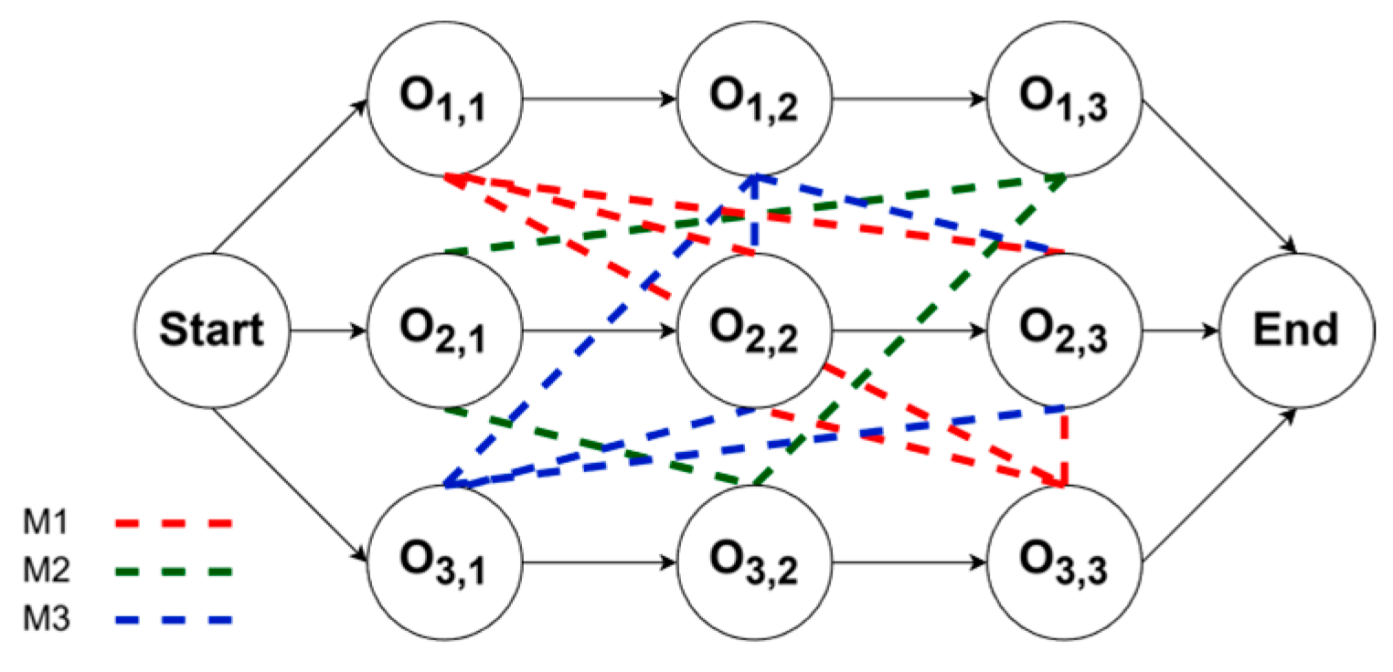
The disjunctive graph provides a standardized modeling framework for FJSP, formally defined as a tuple $G=(\mathcal{V},\mathcal{C},\mathcal{D})$. Figure 1 illustrates the disjunctive graph structure for a 3 × 3 FJSP instance (3 jobs, 3 machines). The node set $\mathcal{V}$ comprises all operation nodes $O_{i,j}$, along with two dummy nodes, representing the start and end of the scheduling process, respectively. The set of conjunctive arcs $\mathcal{C}$ (solid arrows) represents the technological precedence constraints between consecutive operations of the same job, ensuring that $O_{i,j}$ is processed before $O_{i,j+1}$. The set of disjunctive arcs $\mathcal{D}$ (dashed lines) connects pairs of operations that can be processed on the same machine, reflecting the resource constraints and mutual exclusivity.

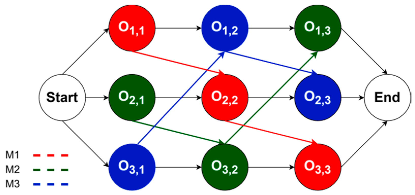
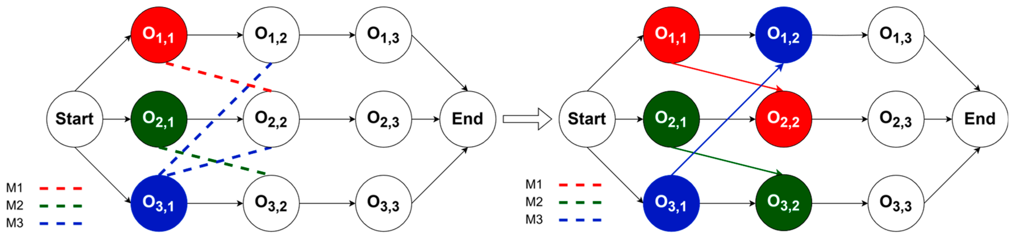
Figure 2 presents a feasible solution derived from the instance. Once the machine assignment and processing sequence are determined, the undirected disjunctive arcs are transformed into directed edges, eliminating cycles in the graph. As shown in Figure 3, the scheduling solution is constructed dynamically. Specifically, when an operation is assigned to a machine, the disjunctive arcs associated with that machine are retained and oriented to indicate the processing order (colored solid arrows), while arcs connecting to unselected machines are removed. The length of the longest path from node start to node end in the final graph corresponds to the makespan of the schedule.

3.3. Markov Decision Process

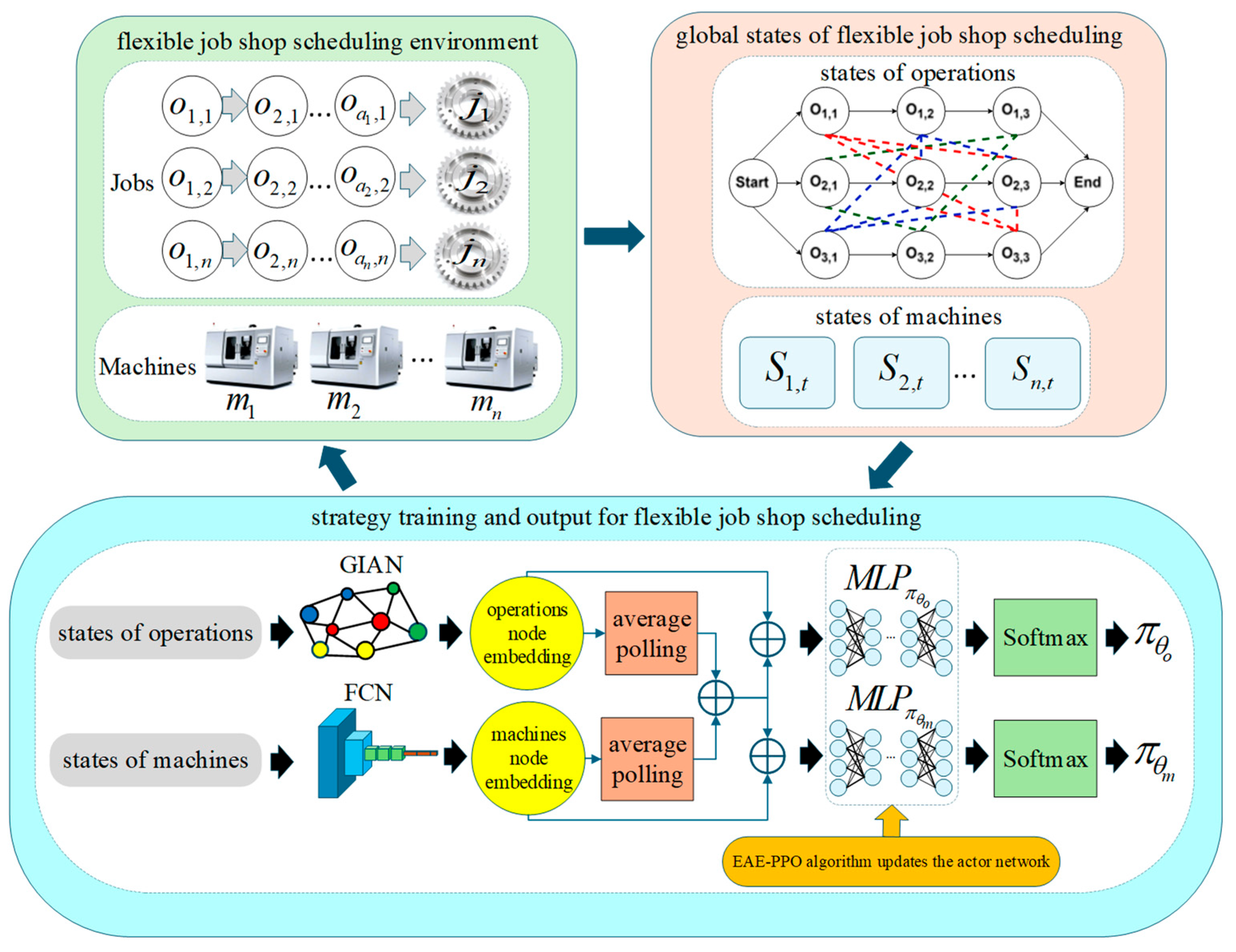
This study transforms the FJSP into a sequential decision-making problem via a Markov Decision Process (MDP). The proposed framework integrates an improved Graph Neural Network with EAE-PPO to optimize the scheduling policy. As illustrated in Figure 4, the system architecture operates as follows: within the scheduling environment (left), circles represent individual operations linked by grey block arrows indicating technological precedence constraints toward the completion of jobs (symbolized by gear icons). During the representation learning phase, the GIAN (depicted as a node-link structure) extracts topological features from these operation nodes, while a fully connected network (represented as sequential blocks) simultaneously encodes machine states. Black long arrows throughout the diagram indicate the direction of information flow. Finally, these two types of features are fused and fed into a dual-path Actor network to jointly learn operation selection and machine assignment policies; a Multilayer Perceptron outputs the action probability distribution, and scheduling decisions are executed based on a greedy policy. The specific definitions of states, actions, rewards, and policies within this MDP are detailed below.

(1)

States

To avoid ambiguity, we adopt distinct notation for different state components: $S_t^o$ denotes the operation state (features of operation nodes $O_{i,j}$), $S_t^m$ denotes the machine state (resource occupancy), and $S_t$ represents the global state combining both components.

The global state $S_t$ at decision step t is constructed by jointly considering the operation state $S_t^m$ and the machine state $S_t^m$ to reflect the dynamic characteristics of workshop. The operation state $S_t^o$ corresponds to the feature vectors of operation nodes in the disjunctive graph. The raw features of each operation node $O_{i,j}$ are defined as shown in Equation (2):

$$S_t^o=\{L{B}_t(O_{i,j}),I_t(O_{i,j})\}$$

(2)

where $L{B}_t(O_{i,j})$ presents the estimated earliest completion time of the operation. For scheduled operations, this value equals the actual completion time; for unscheduled operations, it is recursively calculated based on the completion time of the preceding operation $O_{i,j-1}$ and the minimum processing time $p_{i,j}^k$, where the $p_{i,j}^k$ refers to the processing time of $O_{i,j}$ on $m_k$ shown in Equation (3):

$$L{B}_t(O_{i,j})=L{B}_t(O_{i,j-1})+min(p_{i,j}^k)$$

(3)

where $I_t(O_{i,j})$ serves as a binary status indicator, taking a value of 1 if the operation $O_{i,j}$ has been scheduled, and 0 otherwise. The machine state $S_t^m$ captures the resource occupancy status, defined by Equation (4):

$$S_t^m=\{T_t(m_k),p_{i,j}^k\}$$

(4)

where $T_t(m_k)$ represents the time point at which the machine $m_k$ will complete its current processing task at step t.

(2)

Actions

To address the dual flexibility of FJSP, the action space at each decision step t is decomposed into two components: the operation selection action $a_{o,t}$ and the machine assignment action $a_{m,t}$. The agent first selects an operation $a_{o,t}$ from the set of feasible operations $A_{o,t}$ (operations whose predecessors have been completed). Subsequently, it selects a machine $a_{m,t}$ from the available machine set $A_{m,t}$ which is compatible with the chosen operation.

The overall policy ${\pi }_{\theta }\left(a_t\mid S_t\right)$ is accordingly decomposed into an operation sub-policy ${\pi }_{\theta }^o\left(a_{o,t}\mid S_{o,t}\right)$ and a machine sub-policy ${\pi }_{\theta }^m\left(a_{m,t}\mid a_{o,t},S_{m,t}\right)$. After executing the composite action $a_t=\left(a_{o,t},a_{m,t}\right)$, the system updates to the next state $S_{t+1}$ based on processing times and resource constraints.

(3)

Reward function

The reward serves as a scalar feedback signal to the agent, reflecting the quality of the scheduling decision. In this study, the immediate reward is designed as a composite function of the operation reward and the machine reward, as shown in Equation (5):

$$R_t=r_{t,o}+r_{t,m}$$

(5)

The operation reward $r_{t,o}$ aims to minimize the makespan and is defined as the difference in the estimated maximum completion time between two consecutive steps:

$$r_{t,o}=C(S,t)-C(S,t+1)$$

(6)

If $r_{t,o}>0$, it indicates that the action has effectively shortened the overall completion time, resulting in a positive reward; otherwise, a penalty is imposed. The machine reward $r_{t,m}$ is introduced to promote efficient and balanced equipment utilization. It is determined jointly by the average machine utilization rate $\overline{U}(s,t)$ and the load balancing index ${\sigma }_U(s,t)$, as defined in Equation (7):

$$r_{t,m}=\overline{U}(s,t)-{\sigma }_U(s,t)$$

(7)

The average machine utilization rate $\overline{U}(s,t)$ is calculated as follows:

$$\overline{U}(S,t)={\displaystyle \frac{1}{k}}{\displaystyle \sum _{m=1}^k\frac{{\displaystyle {\sum }_{o\in O_m}{p}_o}}{C_{max}(S_t)}}$$

(8)

where $p_o$ represents the set of operations already scheduled on machine $m_k$. A higher $\overline{U}(s,t)$ indicates less idle time. The load balancing index ${\sigma }_U(s,t)$ is defined as the standard deviation of utilization:

$${\sigma }_U(S,t)=\sqrt{{\displaystyle \frac{1}{k}}{\displaystyle \sum _{m=1}^k{(U_m(S,t)-\overline{U}(S,t))}^2}}$$

(9)

A smaller ${\sigma }_U(s,t)$ indicates a more uniform distribution of workload across machines, preventing single-machine overloads that could prolong the makespan.

4. Proposed Method

4.1. Algorithm Design

By using Lagrange polynomial interpolation to create a smooth exploration curriculum, our EAE-PPO provides a predefined yet flexible exploration schedule that guides the single agent from aggressive exploration to precise exploitation, a strategy not explored in the aforementioned works. While adaptive mechanisms for PPO have been explored, our EAE-PPO differs fundamentally in its approach and objective. Unlike offline hyperparameter optimization methods that produce static configurations [29], our approach implements online, dynamic entropy adjustment that continuously responds to training progress. Furthermore, unlike methods that rely on task-specific feedback, such as success rates or multi-agent signals like team-average entropy [31,32], our mechanism is driven by the overall training progress. This makes it particularly suitable for combinatorial optimization problems like FJSP, which lack clear episodic success metrics or multiple agents.

The core idea of EAE-PPO is to dynamically adjust the entropy coefficient during training to balance exploration and exploitation. In early training stages, a high entropy coefficient encourages the agent to explore diverse scheduling strategies, mimicking the aggressive search behavior of SAC. As training progresses, the entropy coefficient gradually decreases, allowing the agent to exploit the discovered high-quality solutions with precision. Unlike standard PPO’s linear decay or SAC’s fixed entropy target, our mechanism uses a structured curriculum combining linear interpolation (for monotonic decay) and Lagrange polynomial interpolation (for flexible nonlinear adjustment), enabling smooth transitions between exploration and exploitation phases while maintaining the stability guarantees of the PPO trust region. This paper proposes an adaptive entropy adjustment mechanism based on Lagrange Polynomial Interpolation to achieve state-dependent exploration intensity regulation within the PPO framework. This approach aims to enhance exploration capability while maintaining training stability. 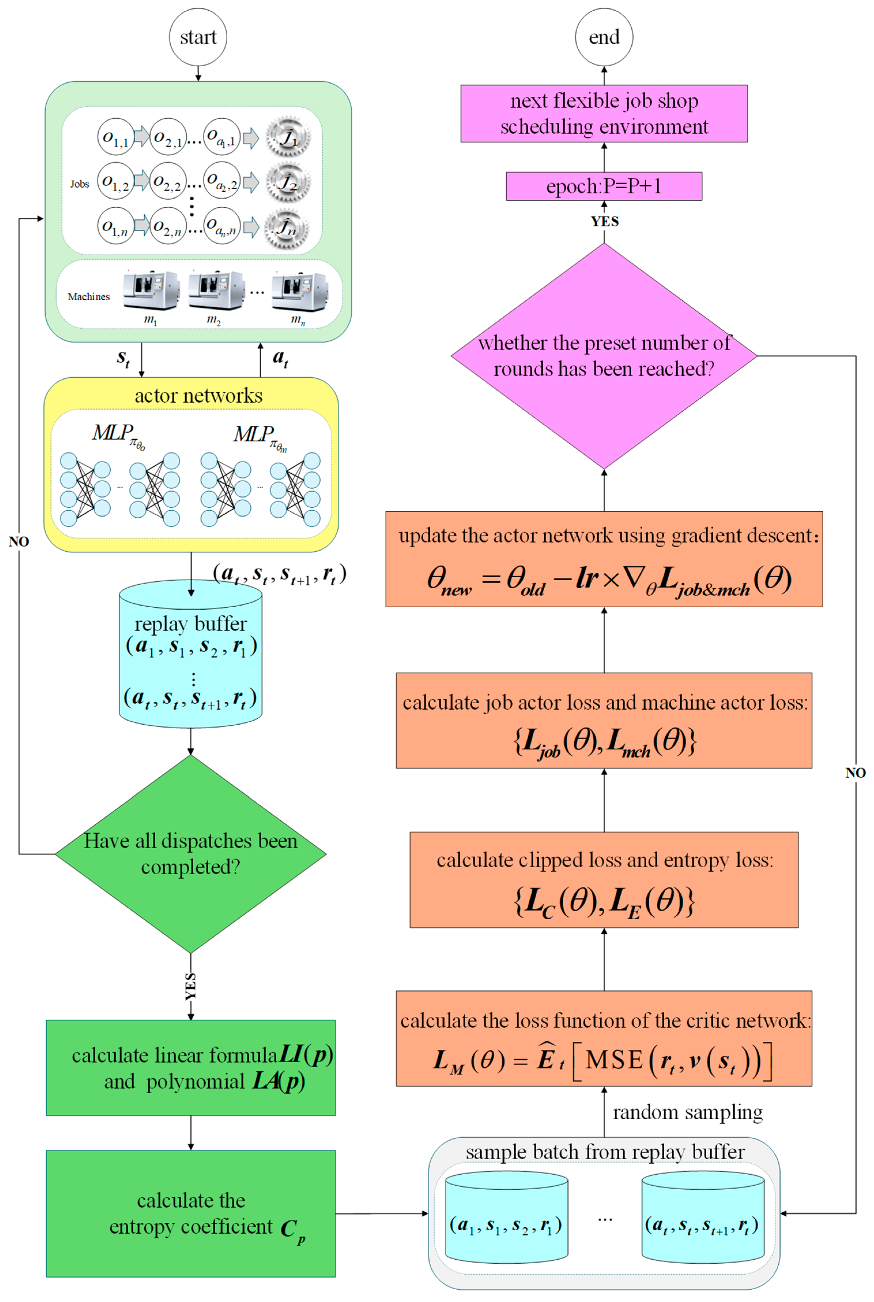The workflow of the proposed mechanism is illustrated in Figure 5. Given an FJSP instance, the policy network (Actor) first generates a complete schedule. Subsequently, the accumulated experience trajectories are leveraged to update the network parameters via the EAE-PPO algorithm. To modulate the exploration–exploitation trade-off, the entropy coefficient is initialized with a basic decay trend defined by linear interpolation:

$$LI(p)=c_s+(c_e-c_{\mathrm{s}})\times p$$

(10)

where $p$ denotes the ratio of the current training episode to the total number of episodes, while $c_s$ and $c_e$ represent the initial and terminal entropy coefficients, respectively. To further augment the flexibility of exploration regulation, Lagrange polynomial interpolation is superimposed upon the linear baseline to construct a nonlinear entropy adjustment curve:

$$LA(p)={\displaystyle \sum _i{y}_i}{\displaystyle \prod _{j\ne i}\frac{(p-p_j)}{(p_i-p_j)}}$$

(11)

$$\begin{array}{l}\{y_1,\dots ,y_n\}\in \mathcal{U}(c_s,c_e)\\ \{p_1,\dots ,p_n\}\in \mathcal{U}(0,1)\end{array}$$

(12)

Here, $\{(y_1,p_1),(y_2,p_2),\dots ,(y_n,p_n)\}$ constitutes a set of key control points defining the adjustment trajectory. The time nodes $p_i$ mark critical phases for entropy adjustment, while $y_i$ specifies the target entropy values at these nodes, thereby governing the exploration intensity at specific training stages. The values are determined via uniform distribution sampling, denoted as $\mathcal{U}$.

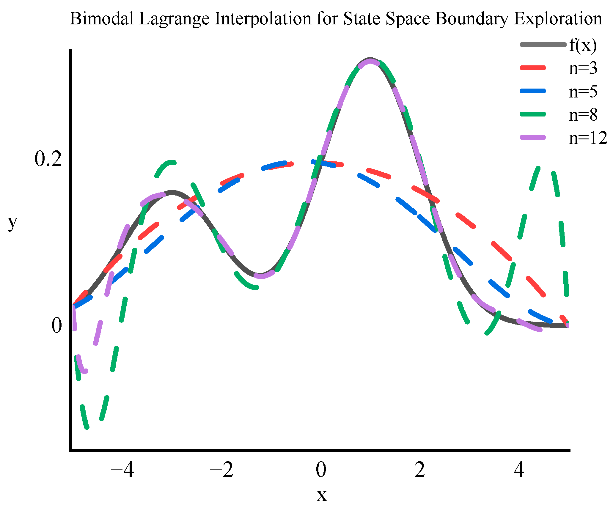
Figure 6 illustrates the approximation characteristics of Lagrange polynomials of varying orders on an example bimodal function. The black solid line represents the target function, while colored dashed lines depict polynomials constructed with different numbers of interpolation nodes. It is observed that low-order polynomials (n = 3, 5) ensure stability at interval boundaries but lack the capacity to capture complex bimodal structures, potentially resulting in insufficient exploration during intermediate phases. Conversely, high-order polynomials (n = 8, 12), while offering superior approximation accuracy, exhibit severe oscillations (Runge’s phenomenon) at the boundaries. Such oscillations can induce sharp spikes in policy gradient variance, destabilizing the training process. Consequently, a moderate polynomial order is selected to strike an equilibrium between encouraging novel solution exploration and maintaining update stability.

The final entropy coefficient $C_p$ is formulated by synthesizing the linear and polynomial components. Furthermore, the second derivative of the Lagrange polynomial is incorporated to sense curvature changes, thereby enhancing the adaptability of the exploration strategy:

$$C_p=LI(p)(1-p^d)+LI(p){(1-p)}^d{\displaystyle \frac{{\partial }^{2}LA(p)}{\partial p^2}}$$

(13)

This composite strategy ensures high exploration rates in the early training stages and facilitates a smooth transition in the mid-to-late stages through nonlinear decay and curvature perception, effectively curbing premature convergence.

Following the entropy adjustment, the network optimization involves minimizing a composite loss function. The critic network minimizes the mean squared error between the estimated value and the returns:

$${\mathcal{L}}_V(\theta )={\mathbb{E}}_{(s,a)~\mathcal{B}}\left[{\left(V_{\theta }(\varphi )-\widehat{R}(s,a)\right)}^2\right]$$

(14)

The actor network is optimized by maximizing the PPO objective, which incorporates a clipped surrogate objective to prevent excessive policy updates, augmented by the cross-entropy loss for action prediction:

$${\mathcal{L}}_C(\theta )={\mathbb{E}}_{(s,a)~\mathcal{B}}\left[\min \left\{{\displaystyle \frac{\pi (a_t|s_t)}{{\pi }_{old}(a_t|s_t)}}\widehat{A}(s,a),clip\left({\displaystyle \frac{\pi (a_t|s_t)}{{\pi }_{old}(a_t|s_t)}},1-ϵ,1+ϵ\right)\widehat{A}(s,a)\right\}\right]$$

(15)

$${\mathcal{L}}_E(\theta )=-{\displaystyle \sum _a\pi }(a_t|s_t)\log \pi (a_t|s_t)$$

(16)

The total loss function governing the Actor networks (encompassing both Operation and Machine Assigner modules) aggregates the policy objective, value error, and entropy term:

$$L\left(\theta \right)={\mathcal{L}}_C\left(\theta \right)+{\mathcal{L}}_V\left(\varphi \right)-C_P{\mathcal{L}}_E\left(\theta \right)$$

(17)

Once the total loss is computed, the parameters ${\theta }_m$ and ${\theta }_o$ of the Actor networks are updated via gradient descent. This iterative process persists until the preset number of gradient update steps is reached, at which point the model proceeds to the subsequent FJSP environment for continued optimization.

Algorithm 1 summarizes the complete training procedure of the proposed EAE-PPO framework. The algorithm integrates three key components: (1) trajectory collection via the current policy, where the agent interacts with the FJSP environment to gather experience; (2) dynamic entropy coefficient adjustment using linear and Lagrange polynomial interpolation, which adaptively regulates exploration intensity based on training progress; and (3) policy optimization through clipped surrogate objectives with entropy regularization, ensuring stable parameter updates within the PPO trust region. This structured workflow ensures that the agent remains stable on-policy learning while adaptively balancing exploration and exploitation throughout the training process. The entropy adjustment mechanism is executed once per training instance, dynamically modulating the exploration intensity to enable a smooth transition from aggressive search in early stages to precise exploitation in later stages.

Algorithm 1: EAE-PPO Training Framework

1: Input: Maximum epochs $E$, Batch size $B$, Total training instances $\left|D\right|$, Number of PPO update epochs $K$, Discount factor $\gamma$, Clipping threshold $\epsilon$, Entropy coefficient $c_s$, Final coefficient $c_e$, Polynomial degree $d$, Actor network parameters ${\theta }_{job}$ and ${\theta }_{mch}$, Critic network parameters $\varphi$. 2: for epoch = 1 to $E$ 3:   Fetch a batch of training instances from data loader (each instance is an FJSP problem) 4:   for each instance $b$ = 1 to $B$ in the batch do 5:        Reset environment, obtain initial state, Initialize trajectory lists 6:           while environment is not terminal do 7:            Select job action ${\theta }_{job}$ using old policy ${\pi }_{{\theta }_{job}}^{old}$ and log probability $log\left({\pi }_{{\theta }_{job}}^{old}\right)$ 8:            Select machine action ${\theta }_{mch}$ using old policy ${\pi }_{{\theta }_{mch}}^{old}$ and log probability $log\left({\pi }_{{\theta }_{mch}}^{old}\right)$ 9:            Execute action ($a_{job}$,$a_{mch}$), receive reward $r$, next state $s_{t+1}$ 10:          Store transition ($s$,$a_{job}$,$a_{mch}$,$r$,$log\left({\pi }_{{\theta }_{job}}^{old}\right)$, $log\left({\pi }_{{\theta }_{mch}}^{old}\right)$) into buffer 11:          Update current state $s\leftarrow s_{t+1}$ 12:          end while 13:      Compute current step index: $t$ = epoch × $\left|D\right|$+$b$ 14:      EAE-PPO Entropy Coefficient Computation: 15:      Normalized progress: $p$ = ${\displaystyle \frac{t}{T_{total}}}$ 16:      Compute linear interpolation component: $LI(p)$ 17:      Compute entropy coefficient: $C_p=LI(p)(1-p^d)$ 18:      Compute the Lagrange polynomial: $LA(p)$ 19:      Compute curvature term: $Cur=LI(p){(1-p)}^d{\displaystyle \frac{{\partial }^{2}LA(p)}{\partial p^2}}$ 20:      Update current entropy coefficient: $C_p\leftarrow C_p+Cur$ 21:         for each PPO update epoch $k$ = 1 to $K$ do 22:           Sample a batch of trajectories from buffer 23:          Compute discounted returns $\widehat{R}(s,a)$ and advantages $\widehat{A}(s,a)$ 24:           Compute policy ratios: $r_{job}(\theta )$ = ${\displaystyle \frac{\pi (a_t|s_t)}{{\pi }_{old}(a_t|s_t)}}$, similarly $r_{mch}(\theta )$ 25:           Compute clipped surrogate objectives: ${\mathcal{L}}_C^{job}(\theta )$ and ${\mathcal{L}}_C^{mch}(\theta )$ 26:           Compute value loss: ${\mathcal{L}}_V(\theta )$ 27:            Compute policy entropies: ${\mathcal{L}}_C^{job}(\theta )$ and ${\mathcal{L}}_C^{mch}(\theta )$ 28:            EAE-PPO total loss: 29:            $L^{job}(\theta )={\mathcal{L}}_C^{job}(\theta )+{\mathcal{L}}_V\left(\varphi \right)-C_P{\mathcal{L}}_E^{job}(\theta )$ 30:            $L^{mch}(\theta )={\mathcal{L}}_C^{mch}(\theta )+{\mathcal{L}}_V\left(\varphi \right)-C_P{\mathcal{L}}_E^{mch}(\theta )$ 31:            Perform gradient update on ${\theta }_{job}^{old}\leftarrow {\theta }_{job}$ and ${\theta }_{mch}^{old}\leftarrow {\theta }_{mch}$ 32: Output: Optimized policy parameters $({\theta }_{job},{\theta }_{mch})$

4.2. Graph Isomorphism Attention Network

Traditional GNNs rely on local message-passing mechanisms, which struggle to capture long-range dependencies between operations crucial for global optimization. To capture how a bottleneck machine in late stages affects early operation assignments, standard GIN would require very deep layers (>10), leading to over-smoothing [34]. Conversely, pure Transformers assume fully connected graphs, lacking the structural inductive bias to respect FJSP’s strict precedence constraints. Our GIAN bridges this gap by combining: GIN layers for local topology encoding (preserving operation precedence) and self-attention for global context capture (modeling resource contention) This hybrid architecture is specifically designed for the disjunctive graph structure of FJSP, where local constraints and global dependencies coexist. 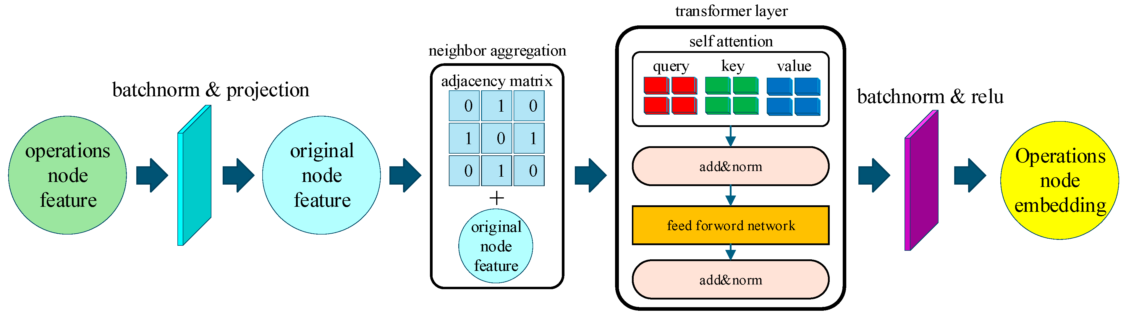As illustrated in Figure 7, GIAN is designed to embed the complex state of the scheduling disjunctive graph and extract deep node features that encapsulate both local topology and global context.

At each decision step, the scheduling environment is represented as a disjunctive graph. The embedding process proceeds as follows:

First, raw node features are preprocessed via batch normalization to standardize each dimension, followed by a linear projection layer that maps the normalized features $h_i^{(k-1)}$ from the input dimension to the hidden dimension required for aggregation. Subsequently, the processed features undergo neighborhood information aggregation within the GIN framework. The update rule is defined as follows:

$$H_i=(1+ϵ)\cdot h_i^{(k-1)}+{\displaystyle \sum _{j\in \mathcal{N}(i)}{h}_j^{(k-1)}}$$

(18)

Here, $\mathcal{N}(i)$ denotes the set of neighboring nodes for node i, and $ϵ$ is a learnable parameter or a fixed scalar. To ensure numerical stability, a mean aggregation method is adopted:

$${\displaystyle \sum _{j\in \mathcal{N}(i)}{h}_j^{(k-1)}}=D^{-1}\cdot ad{j}_x\cdot h_i^{(k-1)}$$

(19)

where $D$ is the degree of node i, used to normalize the neighborhood relationships.

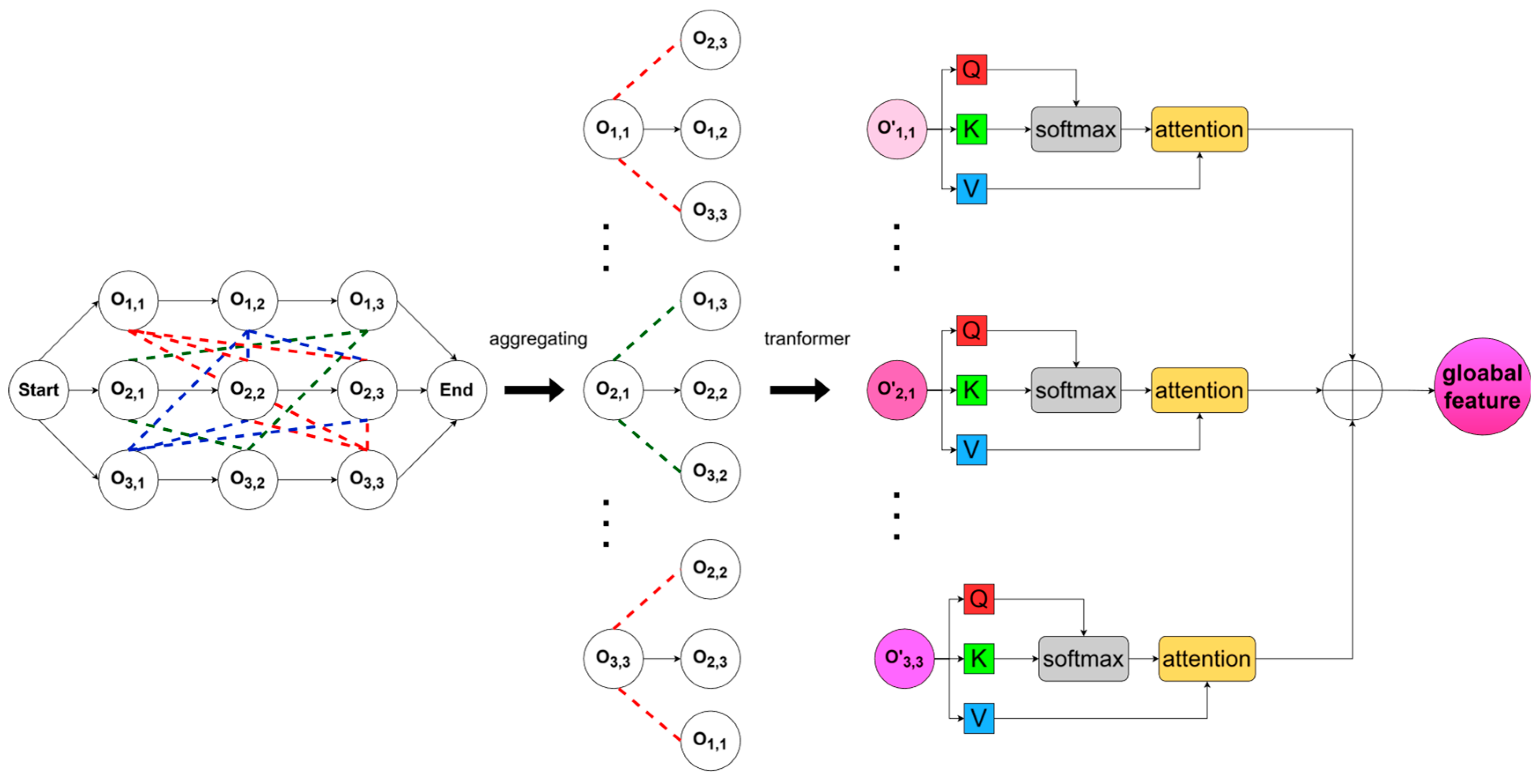
To capture global dependencies, the aggregated node representation sequence $\{H_1,H_2,\dots ,H_2\}$ is fed into a self-attention layer. The module first projects each node representation into Query ($Q$), Key ($K$), and Value ($V$) spaces, which are three distinct, learnable weight matrices,$(W^Q,W^K,W^V)\in {ℝ}^{d_L\times d_F}$, where $d_L$ is the hidden dimension and $d_F$ is the feature dimension. The projection is performed as follows:

$$Q=H\cdot W^Q,K=H\cdot W^K,V=H\cdot W^V$$

(20)

The attention mechanism calculates the similarity between queries and keys, generating attention weights via the Softmax function to produce the output representation:

$$\mathrm{Attention}(Q,K,V)=Softmax\left({\displaystyle \frac{Q{K}^T}{\sqrt{d_F}}}\right)V$$

(21)

Finally, a feedforward neural network with residual connections, layer normalization, and ReLU activation functions processes the output. As shown in Figure 8, this transformation enables the node embeddings to evolve from containing only local state information to integrating global context from all nodes in the graph. This global representation empowers the scheduling policy to foresee potential resource conflicts and operation delays, thereby generating superior global scheduling solutions.

We analyze the computational complexity of a single GIAN layer, which consists of GIN aggregation and a self-attention mechanism. Let $N$ be the number of nodes (operations) and $F$ be the feature dimension. GIN Aggregation: The complexity is $O(\left|E\right|)$, where $\left|E\right|$ is the number of edges. For sparse scheduling graphs, this is approximately linear with the number of nodes, i.e., $O(N)$. Our implementation uses a standard self-attention mechanism, which has a complexity of $O(N^{2}F)$ due to the all-to-all dot product calculation of the $Q$, $K$, $V$ matrices. The total complexity of a GIAN layer is therefore dominated by the self-attention component, resulting in $O(N^{2}F)$. This represents an increase in computational cost compared to the linear complexity of a standard GIN layer ($O(N)$). However, this trade-off is deliberately made to address a critical limitation of GNNs: the inability to capture long-range dependencies in a single layer. The quadratic complexity allows GIAN to model how a bottleneck machine at the end of the schedule can influence decisions at the very beginning, a global perspective that is crucial for achieving near-optimal solutions. As demonstrated in our ablation study (Section 5.3), this increased representational power leads to significant improvements in scheduling performance, justifying the additional computational cost for offline training. For inference, the execution time remains well within practical limits for real-time decision-making.

4.3. Scheduling Action Prediction

After processing through N layers of the GIAN encoding network, node-level embedding vectors $h_v$ are output. To obtain the global graph representation, a graph pooling operation is performed on the node features:

$$h_{\mathcal{G}}={\displaystyle \frac{1}{\left|\mathcal{O}\right|}}{\displaystyle \sum _{v\in \mathcal{O}}}{h}_v$$

(22)

Based on the features extracted by the GIAN encoder, the decoding phase employs two independent Multi-Layer Perceptrons (MLPs) to predict the operation action scores and machine action scores, respectively:

$$\begin{array}{l}{c}_v^o=ML{P}_{{\pi }_{\theta }}\left(h_v\Vert h_{\mathcal{G}}\Vert u\right)\\ c_k^m=ML{P}_{{\pi }_{\theta }}\left(h_k\Vert h_{\mathcal{G}}\Vert u\right)\end{array}$$

(23)

Here, $u$ is the machine pooling vector output by the machine-encoding FCN network, $h_k$ is the machine node feature, and the symbol∙||∙denotes the concatenation operation. Subsequently, the Softmax activation function is used to normalize the action scores, yielding the probability distributions for operation selection and machine assignment, respectively:

$$\begin{array}{l}{\pi }_{\theta }^o\left(a_{o,t}\mid s_{o,t}\right)=softmax\left(c_v^o\right)\\ {\pi }_{\theta }^m\left(a_{m,t}\mid s_{o,t},a_{o,t}\right)=softmax\left(c_k^m\right)\end{array}$$

(24)

Finally, the agent, according to the probability distributions ${\pi }_{\theta }^o\left(a_{o,t}\mid s_{o,t}\right)$ and ${\pi }_{\theta }^m\left(a_{m,t}\mid s_{o,t},a_{o,t}\right)$, samples from the current set of feasible operations $A_{o,t}$ and the corresponding set of feasible machines $A_{m,t}$, obtaining the operation action $a_{o,t}$ and the machine action $a_{m,t}$, thereby completing one step of the scheduling decision.

5. Experimental Design

Note on notation: In all figures and tables throughout Section 5, the label “Ours” refers specifically to our proposed method, GIAN + EAE-PPO (Graph Isomorphism Attention Network combined with Entropy-Adjusted PPO). For brevity and visual clarity in comparative visualizations, we use “Ours” to denote this complete framework.

5.1. Configuration

The experiments are implemented using Python 3.9 and the PyTorch 1.6.1 framework, running on a computer with an AMD Ryzen 7 5700X @3.70 GHz CPU and 64 GB RAM, NVIDIA GeForce RTX 4060 Ti. To systematically evaluate the performance of the proposed DRL scheduling method, this study designs a comprehensive assessment framework comprising parameter sensitivity analysis, ablation studies, and comparative experiments. First, the impact of key hyperparameters on algorithm performance and stability is investigated to determine the optimal parameter configuration. Second, ablation experiments are conducted to quantitatively analyze the contributions of core components, specifically the encoder modules and exploration mechanisms, validating the effectiveness of the proposed framework. Finally, to confirm the superiority and robustness of the proposed method, it is compared with classic dispatching rules and state-of-the-art DRL methods reported in the recent literature.

The training instances used in this study were generated randomly. For the testing phase, three widely recognized public benchmark datasets are employed [35,36,37]. The Hurink dataset consists of three subsets—Edata, Rdata, and Vdata—characterized by increasing levels of machine flexibility. Specifically, Edata offers limited machine options, whereas Vdata allows almost all operations to be processed on multiple machines. The Brandimarte dataset represents a classic benchmark where the majority of operations possess machine flexibility with varying processing times. The Dauzère–Pérès dataset, while similar to Hurink in processing time characteristics, features a significantly higher average number of operations per job, presenting a challenge in terms of problem scale. To ensure a fair and rigorous comparison, we adopted a multi-faceted approach for hyperparameter settings. For established DRL baselines published in the literature (e.g., HGNN + PPO, DAN + PPO, GAT + SAC), we used the hyperparameter configurations reported in their respective original papers to ensure we are comparing against their validated state-of-the-art performance. For baseline methods constructed by us for direct comparison (i.e., GIN + SAC and GIAN + SAC), we performed hyperparameter tuning under the same computational budget as our proposed method to ensure a fair comparison of the algorithmic components (SAC vs. EAE-PPO). The best heuristic rules (BRs) were selected by testing multiple common dispatching rules and reporting the best result for each dataset. While this hybrid approach may introduce a slight tuning bias for literature-based baselines, we argue that the substantial and statistically significant performance gap observed across 17 diverse problem scales (Section 5.4) strongly suggests that the superiority of our method is driven by its fundamental design rather than minor hyperparameter differences. Testing on these datasets with varying characteristics and complexities allows for a comprehensive verification of the proposed method’s efficiency and generalization.

To ensure reproducibility, all hyperparameters used for the proposed GIAN + EAE-PPO model are detailed in Appendix A (

Table A5. Hyperparameter Settings for GIAN+EAE-PPO.

Category	Hyperparameter	Value
GIAN Encoder	GIAN Layers (Depth)	3
	Hidden Dimension	128
	Attention Heads	1
	Activation Function	ReLU
PPO Algorithm	Learning Rate ($\alpha$)	0.001
	Discount Factor ($\gamma$)	0.99
	GAE Lambda ($\lambda$)	0.95
	Clipping Threshold ($\epsilon$)	0.2
	PPO Update Epochs ($K$)	5
	Batch Size	64
EAE-PPO	Initial Entropy Coeff. ($c_s$)	0.15
	Final Entropy Coeff. ($c_e$)	0.01
	Lagrange Polynomial Degree ($d$)	5
	Control Points ($p$, $y$)	[(0.8, 0.15),(0.6, 0.11),(0.4, 0.07),(0.2, 0.03),(0, 0.01]
Training	Total Episodes	200

). These settings were determined based on the sensitivity analysis presented in Section 5.2 and established best practices from the literature.

5.2. Sensitivity Analysis

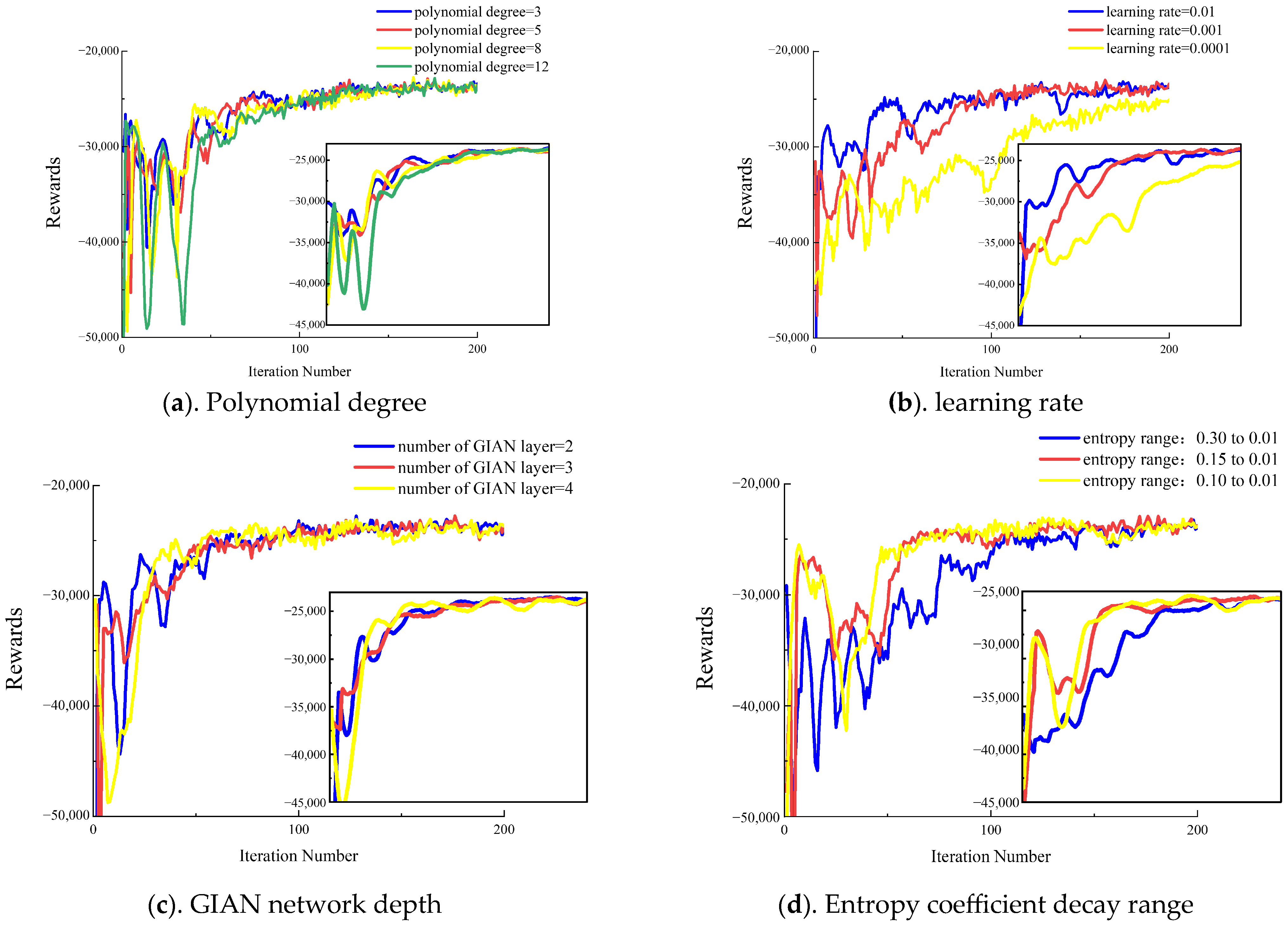
To ensure the robustness of the GIAN model trained with the EAE-PPO algorithm and to determine its optimal configuration, this section conducts a systematic sensitivity analysis on core hyperparameters. The impact of four key hyperparameters—the degree of the Lagrange polynomial, the learning rate, the GIAN network depth, and the entropy coefficient decay range—on the training process is investigated under a consistent baseline configuration. The reward iteration curves for these scenarios are presented in Figure 9, where the subplots in the lower right corner display smoothed training curves using a moving average with a window size of 15 to clearly illustrate convergence trends.

(1)

Polynomial degree

As shown in Figure 9a, the algorithm eventually achieves convergence across different Lagrange interpolation degrees. However, high-degree settings (e.g., d = 8, 12) introduce significant reward fluctuations during the early training stages. This phenomenon can be attributed to the numerical characteristics of high-degree Lagrange interpolation. While the linear interpolation term ensures a fundamental monotonic decay of the entropy coefficient to maintain stability, and the trust region constraint of PPO limits the policy update step size, high-degree polynomials are prone to “Runge’s phenomenon” near the interval ends (corresponding to the initial 50 iterations). This leads to severe oscillations in the entropy coefficient and its second derivative. Consequently, the regulator becomes overly sensitive to the iteration count, amplifying gradient noise when the policy is immature, which manifests as high-frequency oscillations in the reward curve.

(2)

Learning rate

Figure 9b illustrates the training curves under different learning rates. It is observed that learning rates of 0.01 and 0.001 both allow the algorithm to converge near the optimal solution. However, the setting of 0.01 exhibits higher variance in the later stages of convergence, indicating reduced stability compared to 0.001. Conversely, when the learning rate is reduced to 0.0001, although the algorithm eventually approaches the optimal solution, the convergence speed is significantly compromised, with limited performance improvement observed within 200 iterations.

(3)

GIAN network depth

To determine the optimal model complexity, Figure 9c compares the performance of GIAN architectures with varying depths. The results indicate that both 2-layer and 3-layer models converge to similar high-performance levels. However, the 2-layer model exhibits greater fluctuation in the early training phase, whereas the 3-layer model demonstrates the fastest and most stable convergence. Notably, increasing the depth to 4 layers does not yield performance gains; instead, it reduces training stability and results in a slightly inferior final convergence level. This degradation suggests that an overly deep network structure may impede gradient propagation efficiency or lead to overfitting of noise in the early training stages.

(4)

Entropy coefficient decay range

The initial value and decay strategy of the entropy coefficient jointly determine the trajectory of policy exploration intensity. Figure 9d compares three different initial entropy settings. An initial entropy of 0.15 decaying linearly to 0.01 achieves the best balance between sufficient exploration and convergence stability. Increasing the initial entropy to 0.30 results in excessive early-stage exploration, thereby retarding convergence. In contrast, reducing the initial entropy to 0.10 restricts exploration capability, increasing the risk of entrapment in local optima and yielding an inferior final performance.

In summary, the experimental results indicate that while training dynamics vary under different hyperparameter configurations, the proposed method exhibits high stability, with no instances of divergence. The choice of hyperparameters primarily influences convergence speed and smoothness rather than the feasibility of optimization. Based on these findings, the parameter combination that achieves the optimal trade-off among training stability, convergence speed, and scheduling performance is selected. Consequently, all subsequent experiments in this study adopt the following configuration:

• Network Architecture: 3-layer GIAN encoder;
• Optimizer: Adam with a learning rate of 0.001;
• EAE-PPO Parameters: Lagrange interpolation degree d = 5, with the entropy coefficient linearly decaying from 0.15 to 0.01.

5.3. Ablation Experiments

This study conducted ablation experiments to investigate the impact of the Entropy Adaptive Exploration (EAE) strategy and the Graph Isomorphism Attention Network (GIAN) structure on algorithm performance. Three method variants were evaluated: the baseline method (GIN + PPO), the intermediate method introducing only the entropy adaptive exploration module (GIN + EAE-PPO), and the proposed method (GIAN + EAE-PPO).

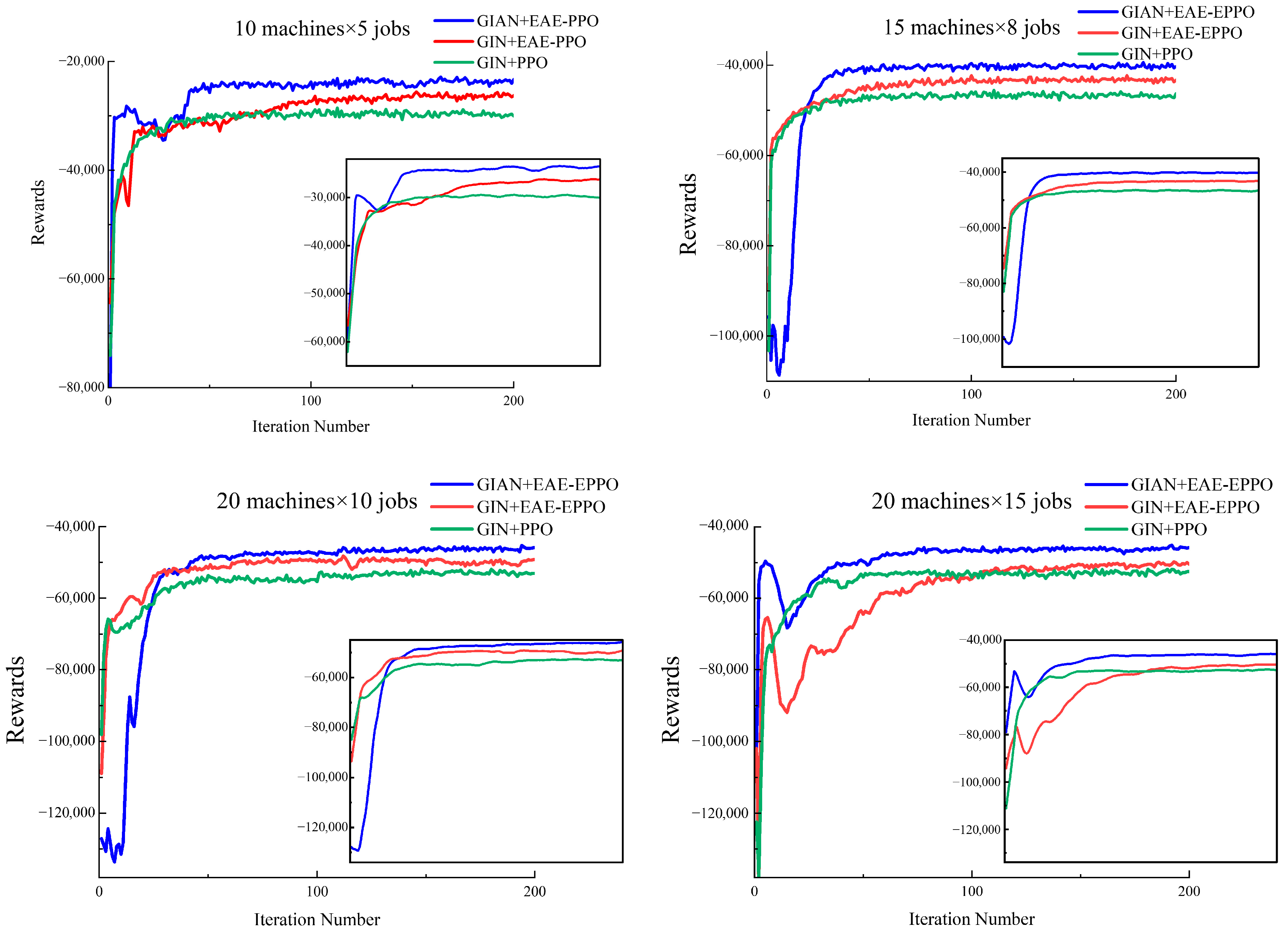
Figure 10 presents the reward iteration curves for these methods across four diverse problem scales: 10 × 5 (small), 15 × 8 (medium), 20 × 10 (large), and 20 × 15 (extra-large). The results reveal a consistent performance hierarchy across all scales: GIAN + EAE-PPO (blue) outperforms GIN + EAE-PPO (red), which in turn surpasses GIN + PPO (green). Specifically, the EAE-PPO module effectively enhances training stability and convergence smoothness, particularly mitigating fluctuations in the later training stages. The GIAN structure accelerates convergence speed and improves final performance, demonstrating superior representation capability compared to the standard GIN encoder. Notably, on the most challenging 20 × 15 scale, despite exhibiting higher variance in early training stages (episodes 0–50) due to the expanded state-action space, GIAN + EAE-PPO still converges to superior performance, demonstrating robust scalability. The smoothed training curves (insets) clearly show that the performance ranking remains stable regardless of problem size, indicating that the contributions of both components are not scale-dependent on the matrices.

To further assess the scheduling performance of different algorithms, the methods were applied to the Brandimarte benchmark dataset.

Table 1. The performance of the three methods in the Brandimarte example.

Scale	Instances	UB	GIN + PPO	GIN + EAE-PPO	GIAN + EAE-PPO
10 × 6	MK01	40	47	42	42
10 × 6	MK02	26	32	32	33
15 × 8	MK03	204	208	204	204
15 × 8	MK04	60	71	70	68
15 × 8	MK05	173	188	179	177
10 × 15	MK06	58	79	77	70
20 × 5	MK07	144	150	154	150
20 × 10	MK08	523	531	541	527
20 × 10	MK09	307	352	338	331
20 × 15	MK10	198	253	249	240
	Gap	0.00%	15.31%	12.85%	10.22%

reports the scheduling results for each instance, where “UB” denotes the known upper bound of the optimal solution, and bold values indicate the best results obtained. The relative scheduling gap (Gap), reflecting the solution quality of the algorithm, is calculated as follows:

$$Gap={\displaystyle \sum _{a\in Instances}}\left({\displaystyle \frac{C_{max}(a)-UB(a)}{UB(a)}}\right)\times 100\%$$

(25)

As shown in Table 1, GIAN + EAE-PPO achieves the best scheduling results in 9 out of 10 instances and demonstrates a significantly lower average Gap (10.22%) compared to GIN + PPO (15.31%) and GIN + EAE-PPO (12.85%). This performance ranking aligns with the convergence trends observed in Figure 10, indicating that the enhanced stability and faster convergence during training effectively translate into superior generalization performance and final scheduling quality. It is noteworthy that the advantages of GIAN + EAE-PPO are particularly prominent on larger-scale or structurally complex instances (e.g., MK06, MK09, MK10). This demonstrates that the combination of the graph isomorphism attention mechanism and the adaptive exploration strategy possesses superior adaptability and scalability for complex scheduling environments.

To comprehensively verify that the observed improvements are not scale-dependent, we systematically evaluated the three methods across diverse problem sizes. Figure 10 presents training dynamics on four representative scales spanning from 10 × 5 to 20 × 15, demonstrating remarkable consistency in convergence patterns. The performance ordering (GIAN + EAE-PPO > GIN + EAE-PPO > GIN + PPO) is preserved across all scales, from the smallest to the largest instances. Table 1 further quantifies these improvements across six distinct scales in the Brandimarte dataset (10 × 6, 15 × 8, 10 × 15, 20 × 5, 20 × 10, 20 × 15). Problem complexity is categorized as follows:

• Small-scale (10 × 6): GIAN + EAE-PPO achieves an average gap of 8.9% (instances MK01-MK02), outperforming GIN + PPO (11.8%) by 2.9 percentage points;
• Medium-scale (15 × 8, 10 × 15, 20 × 5): Average gap of 10.1% (instances MK03-MK07), outperforming GIN + PPO (14.2%) by 4.1 percentage points;
• Large-scale (20 × 10, 20 × 15): Average gap of 10.6% (instances MK08-MK10), outperforming GIN + PPO (17.7%) by 7.1 percentage points.

The consistent improvement margins across all scales (overall average of 5.1 percentage points) demonstrate that both the GIAN encoder and the EAE-PPO mechanism contribute robustly to performance gains regardless of problem complexity. These results validate the effectiveness and necessity of the core components proposed in this study, confirming strong generalizability across diverse problem characteristics.

5.4. Comparison Experiments

To systematically evaluate the comprehensive performance of the proposed method, this study compares it against three categories of representative approaches: heuristic dispatching rules (BRs), PPO-based DRL methods, and SAC-based DRL methods. The specific baselines are detailed as follows:

• PPO-based Methods: Including GIN + PPO [7], HGNN + PPO [8], DAN + PPO [25], and MLP + PPO [27];
• SAC-based Methods: Including GIN + SAC, GIAN + SAC, GAT + SAC [11], and SAC-AMBER [33], which utilizes manual feature extraction and adaptive multi-buffer experience replay;
• Best heuristic rules (BRs): Representing traditional methods; BR denotes the composite dispatching rule (e.g., FIFO + EET, MOPNR + EET, or MWKR + EET) that yields the best performance on the respective dataset;

Table A1. Makespan of different methods based on the Brandimarte dataset.

Scales	Instances	UB	BR	GIN+ PPO	HGNN+ PPO	DAN+ PPO	MLP+ PPO	GAT+ SAC	SAC amber	GIN+ SAC	GIAN+ SAC	Ours
10 × 6	MK01	40	49	47	49	43	44	44	46	45	43	42
10 × 6	MK02	26	43	30	43	29	31	31	30	30	31	30
15 × 8	MK03	204	205	204	216	204	211	207	223	204	204	204
15 × 8	MK04	60	78	76	75	69	78	69	80	71	68	67
15 × 8	MK05	173	184	178	190	176	183	177	180	185	182	177
10 × 15	MK06	58	92	79	103	86	74	77	72	79	73	69
20 × 5	MK07	144	214	152	212	148	156	151	163	158	154	149
20 × 10	MK08	523	541	541	523	523	524	531	526	531	531	527
20 × 10	MK09	307	350	335	349	335	326	334	339	334	339	331
20 × 15	MK10	198	278	236	264	230	241	245	253	254	247	237
	Gap	0.00%	28.98%	13.60%	30.04%	11.21%	13.25%	11.96%	15.31%	13.77%	11.48%	8.51%

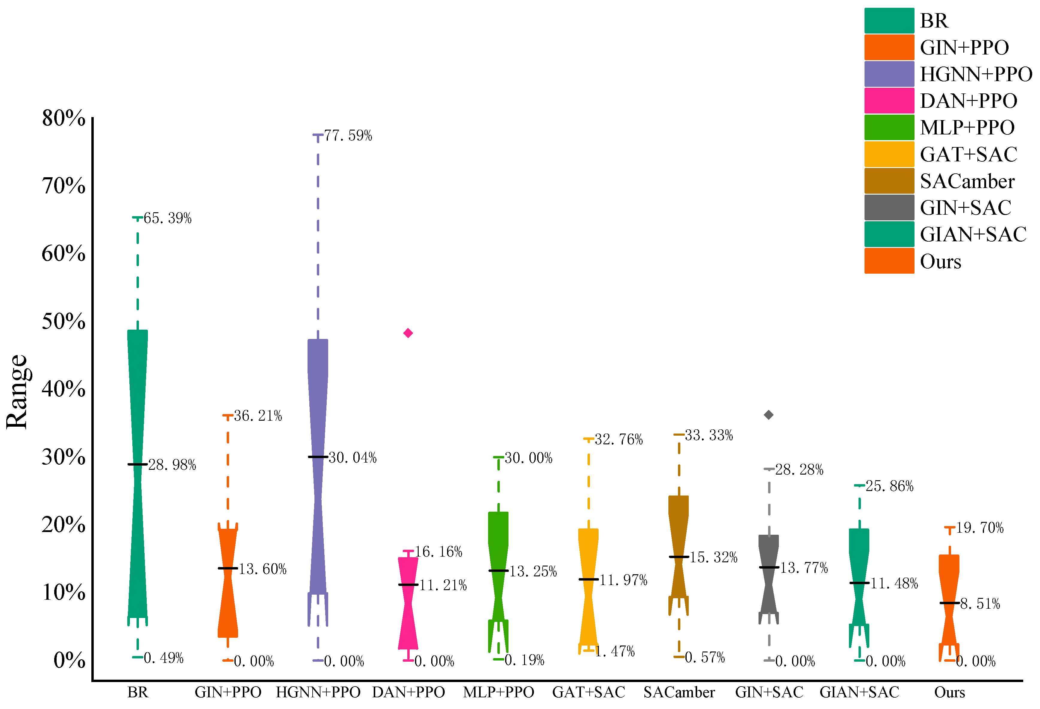
and Figure 11 present the average scheduling gap (Gap) and the boxplot distributions for the Brandimarte dataset, where the diamonds above the boxes represent outliers. The proposed GIAN + EAE-PPO demonstrates significant superiority in both solution quality and stability, achieving a Gap of 8.51%. This performance not only significantly surpasses the traditional heuristic rules but also outperforms all PPO-based and SAC-based variants.

Regarding SAC-based methods, distinct limitations are observed. SAC-AMBER exhibits a larger average gap compared to deep-network-based SAC methods, highlighting the insufficiency of manual feature extraction relative to deep neural representations. A detailed comparison between GIN + SAC and GIN + PPO reveals a critical characteristic: although GIN + SAC achieves a lower average gap, it exhibits multiple statistical outliers (marked as red dots in Figure 11), indicating occasional catastrophic performance degradation. Specifically, the outliers of GIN + SAC extend beyond 1.5 × IQR from the upper quartile, with the worst-case gap reaching 32%, significantly higher than its average performance. In contrast, GIN + PPO, despite having a higher average gap, demonstrates more predictable behavior with fewer outliers. This suggests that while SAC’s maximum entropy framework can discover high-quality solutions, it lacks the robustness guarantees necessary for reliable deployment in production environments.

Furthermore, when SAC is combined with more complex architectures (GIAN + SAC and GAT + SAC), a specific phenomenon emerges: while the distances between the extremes (edges) and quartiles are narrowed—indicating suppression of extreme outliers—the interquartile range (IQR) actually widens compared to GIN + SAC. This reveals a key finding: combining SAC with complex feature extraction does not eliminate instability but systematically shifts it. The powerful representation capabilities constrain instability from the distribution boundaries to the core region, increasing the variance of the middle 50% of results. Consequently, the instability is internalized from the randomness of exploration into the volatility of convergence. In contrast, GIAN + EAE-PPO exhibits the most compact boxplot positioned at the lowest level, demonstrating that the proposed combination of graph attention and adaptive entropy regulation successfully achieves a dual improvement in solution quality and algorithmic robustness.

Table A2. Makespan of different methods based on the Hurink dataset.

Scales	Instances	UB	BR	GIN + PPO	HGNN + PPO	DAN + PPO	MLP + PPO	GIN + SAC	GIAN + SAC	Ours
10 × 5	la(1–5)	531	617	627	593	592	610	622	610	573
15 × 5	la(6–10)	808	874	882	869	857	872	898	883	845
20 × 5	la(11–15)	1051	1134	1145	1118	1120	1127	1143	1122	1098
10 × 10	la(16–20)	732	860	872	826	833	812	850	836	810
15 × 10	la(21–25)	841	1050	1036	959	967	978	1042	1017	979
20 × 10	la(26–30)	1091	1276	1283	1229	1223	1226	1268	1264	1216
30 × 10	la(31–35)	1578	1738	1747	1697	1664	1712	1735	1724	1687
15 × 15	la(36–40)	1057	1249	1259	1216	1203	1182	1258	1235	1179
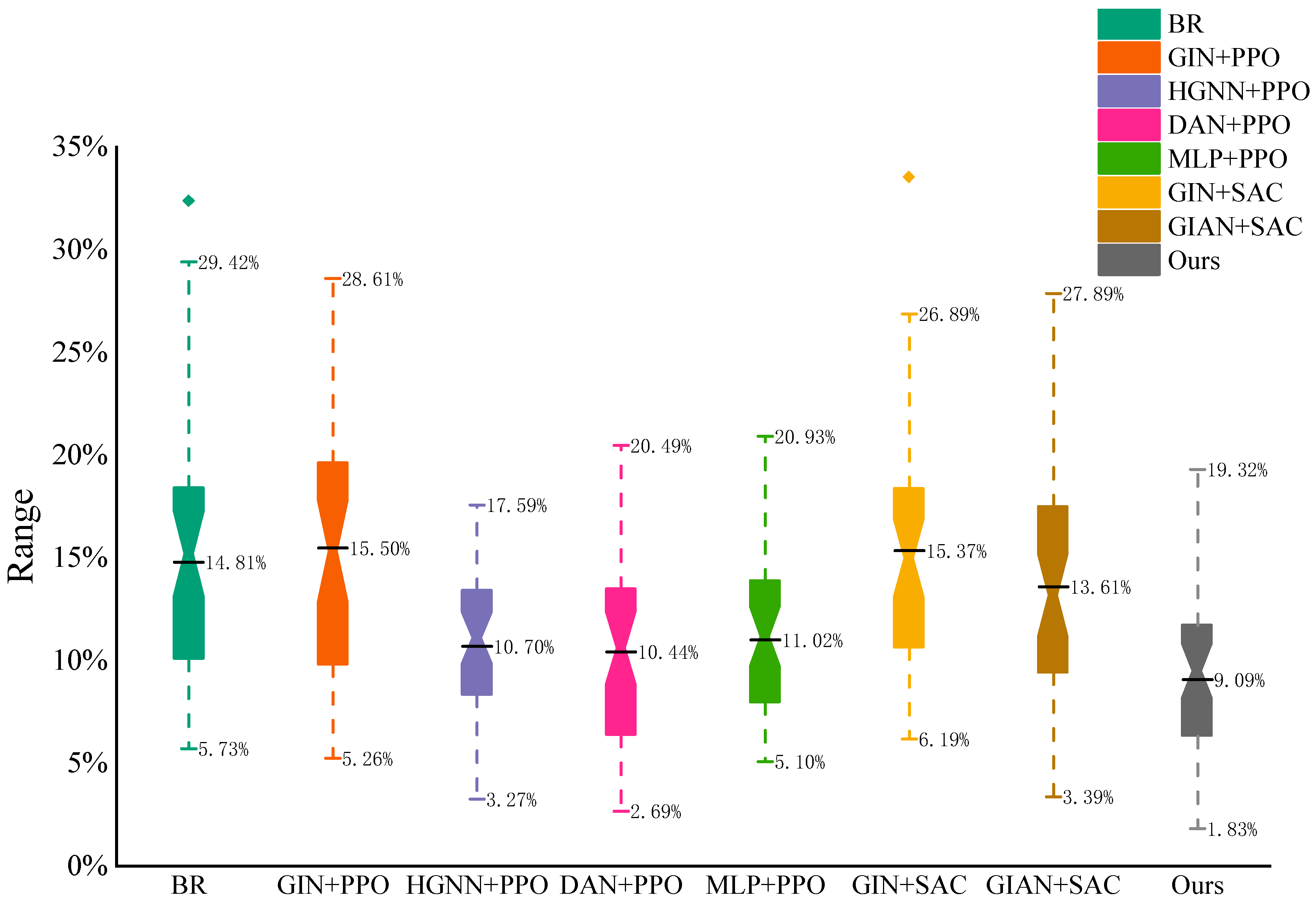
	Gap	0.00%	14.81%	15.50%	10.70%	10.44%	11.02%	15.37%	13.61%	9.09%

and Figure 12 illustrate the generalization performance on the Hurink benchmark. The proposed method achieves the best overall performance with an average gap of 9.09%, significantly outperforming BR (14.81%), HGNN + PPO (10.70%), and DAN + PPO (10.44%). This demonstrates exceptional adaptability across varying problem scales (from 10 × 5 to 30 × 10). Conversely, SAC-based methods perform poorly, with GIN + SAC and GIAN + SAC achieving gaps of only 15.37% and 13.61%, respectively. This suggests that offline policy learning relying solely on maximum entropy struggles to balance exploration and exploitation under the varied flexibility configurations of the Hurink dataset. The compact boxplot of the proposed method in Figure 11 further confirms that the interpolation-based entropy regulation of EAE-PPO effectively suppresses training oscillations, maintaining the ability to escape local optima while ensuring stable convergence.

Table A3. Makespan of different methods based on the Dauzère–Pérè dataset.

Scales	Instances	UB	BR	GIN + PPO	HGNN + PPO	DAN + PPO	MLP + PPO	GIN + SAC	GIAN + SAC	Ours
10 × 25	01a	2518	3138	3109	2847	2865	2947	2983	2998	2855
10 × 25	02a	2231	2416	2603	2478	2533	2495	2558	2709	2429
10 × 25	03a	2229	2359	2366	2294	2306	2320	2425	2662	2304
10 × 25	04a	2503	3109	3093	2856	2879	3037	3001	3146	2898
10 × 25	05a	2216	2525	2573	2473	2415	2496	2570	2608	2412
10 × 25	06a	2203	2410	2508	2262	2331	2286	2382	2547	2299
15 × 25	07a	2283	2897	2857	2736	2643	2820	2977	2783	2711
15 × 25	08a	2069	2321	2386	2191	2230	2259	2376	2336	2247
15 × 25	09a	2066	2170	2209	2097	2104	2155	2185	2203	2141
15 × 25	10a	2291	2786	2805	2635	2664	2721	2819	2810	2651
15 × 25	11a	2063	2401	2356	2227	2210	2206	2282	2358	2260
15 × 25	12a	2034	2203	2186	2090	2094	2157	2202	2196	2121
20 × 25	13a	2260	3044	2811	2739	2622	2755	2811	2811	2696
20 × 25	14a	2167	2347	2353	2218	2224	2277	2467	2383	2313
20 × 25	15a	2167	2325	2385	2193	2197	2202	2318	2343	2254
20 × 25	16a	2255	2821	2861	2723	2737	2680	2926	2916	2696
20 × 25	17a	2141	2356	2365	2224	2207	2309	2369	2450	2280
20 × 25	18a	2137	2308	2363	2185	2172	2216	2344	2312	2231
	Gap	0.00%	15.01%	15.68%	8.89%	8.80%	11.02%	15.22%	16.64%	9.76%

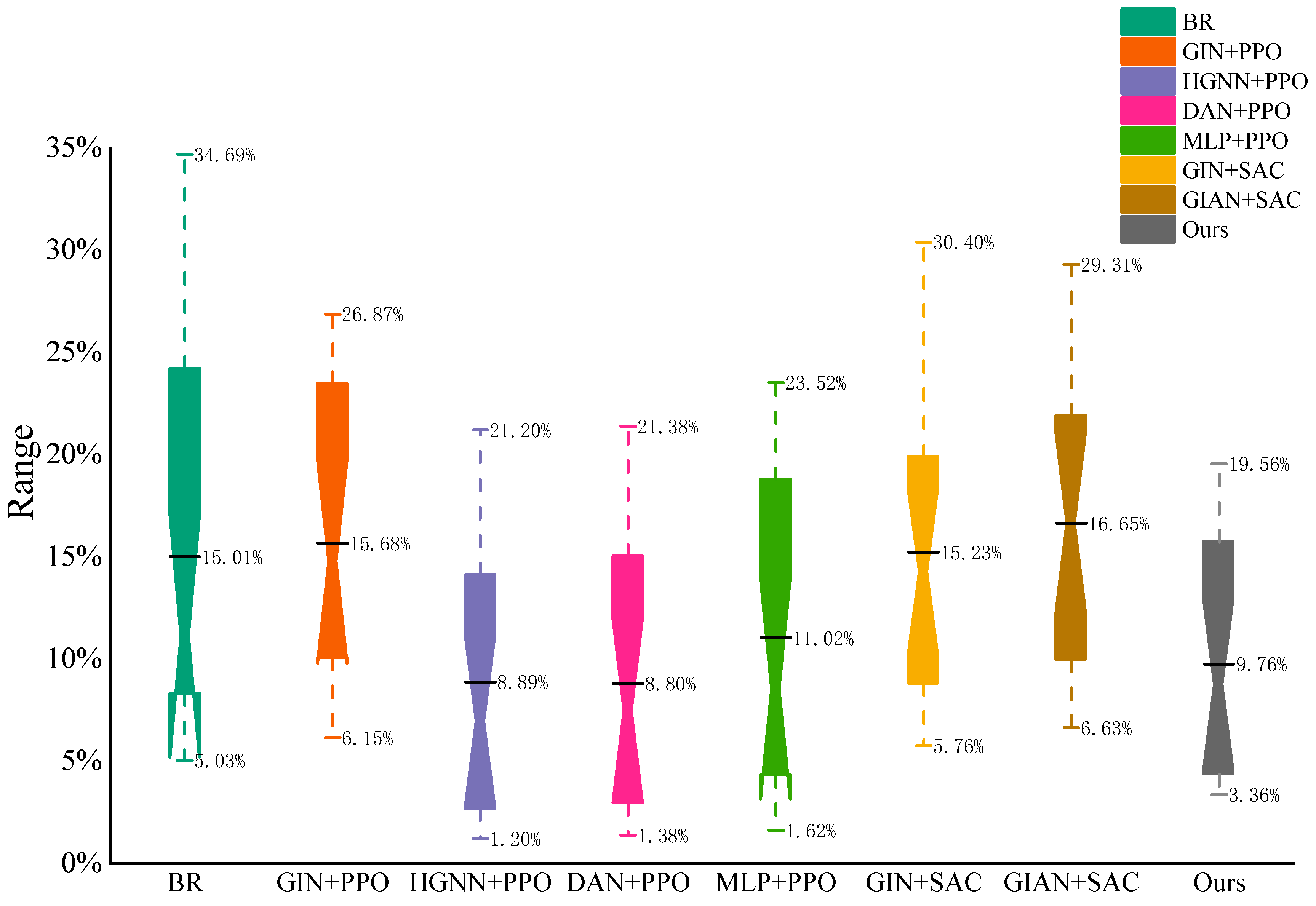
and Figure 13 present the comparison on the Dauzère–Pérès dataset. This dataset is characterized by notably long operation sequences, posing a severe challenge to policy stability and sequential planning over extended decision horizons. The proposed GIAN + EAE-PPO method achieves an average scheduling gap (Gap) of 9.76%, significantly outperforming the best heuristic rule (15.01%) and the baseline GIN + PPO (15.68%). It is observed that HGNN + PPO and DAN + PPO exhibit a slight advantage in average metrics on this specific dataset. However, a comprehensive analysis of the distribution in Figure 12 reveals the superior robustness of the proposed method. The boxplot for GIAN + EAE-PPO is the most compact, featuring significantly shorter distances between the edges and quartiles compared to the competitors. In contrast, SAC-based methods show clear performance degradation with expanded interquartile ranges, and even the PPO-based baselines exhibit greater variability.

This distribution characteristic indicates that GIAN + EAE-PPO possesses superior consistency and output robustness. By effectively capturing long-range dependencies between operations through the GIAN encoder and leveraging the smooth exploration mechanism of EAE-PPO, the agent successfully overcomes cumulative errors and fluctuations inherent in long-sequence decision-making. Consequently, it maintains an efficient search trajectory while effectively avoiding entrapment in local optima or training divergence, which are common pitfalls for maximum entropy frameworks in high-dimensional spaces.

To rigorously assess the superiority of the proposed method, we conducted paired t-tests across all benchmark datasets, with detailed results provided in

Table A4. Paired t-Test Results Across Three Benchmark Datasets.

Dataset	Baseline	Mean Diff.	t-Test	p-Value	Significance
	BR	−0.20474	−3.516	0.00656	**
	GIN + PPO	−0.05088	−3.184	0.04651	*
	HGNN + PPO	−0.21533	−3.226	0.01039	*
	DAN + PPO	−0.02703	−0.887	0.39767	×
Brandimarte	MLP + PPO	−0.04738	−2.684	0.02501	*
	GAT + SAC	−0.03461	−2.743	0.02273	*
	SACamber	−0.06811	−3.276	0.00958	**
	GIN + SAC	−0.05261	−3.113	0.01244	*
	GIAN + SAC	−0.02969	−4.661	0.00118	**
	BR	−0.05723	−11.401	<0.0001	****
	GIN + PPO	−0.06409	−11.293	<0.0001	****
	HGNN + PPO	−0.01616	−3.509	0.00115	**
Hurink	DAN + PPO	−0.01356	−3.058	0.00401	**
	MLP + PPO	−0.01933	−3.791	0.00051	***
	GIN + SAC	−0.06288	−12.789	<0.0001	****
	GIAN + SAC	−0.04524	−11.88	<0.0001	****
	BR	−0.05251	−5.876	<0.0001	****
	GIN + PPO	−0.05924	−10.963	<0.0001	****
	HGNN + PPO	0.00867	1.854	0.08112	†
Dauzère–Pérè	DAN + PPO	0.00953	1.798	0.08991	†
	MLP + PPO	−0.01268	−2.213	0.0408	*
	GIN + SAC	−0.05472	−8.885	<0.0001	****
	GIAN + SAC	−0.06891	−7.724	<0.0001	****

Note: * p < 0.05; ** p < 0.01; *** p < 0.001; **** p < 0.0001; × = not significant; † = marginally significant (p < 0.10) Negative Mean Diff. indicates our method achieves lower makespan (better).

. Results demonstrate that GIAN + EAE-PPO achieves statistically significant improvements over the majority of baselines:

• On the Hurink dataset, our method significantly outperforms all baselines with p < 0.001, including recent DRL methods such as HGNN + PPO (t = −3.509, p = 0.001) and DAN + PPO (t = −3.058, p = 0.004).
• On the Brandimarte dataset, significant improvements are observed over 8 out of 9 baselines. Notably, while the comparison with DAN + PPO does not reach statistical significance (p = 0.398), our method still achieves a lower mean makespan, suggesting comparable or slightly superior performance.
• On the Dauzère dataset, our method significantly outperforms traditional methods (BR, GIN + PPO) and SAC-based approaches (p < 0.0001). The comparisons with HGNN + PPO and DAN + PPO show marginal trends (p = 0.081 and 0.090, respectively), which is expected given that these represent state-of-the-art methods on this specific dataset.

Overall, the statistical analysis confirms that GIAN + EAE-PPO achieves robust and significant performance gains across diverse problem scales and flexibility configurations, validating its effectiveness as a general-purpose FJSP solver.

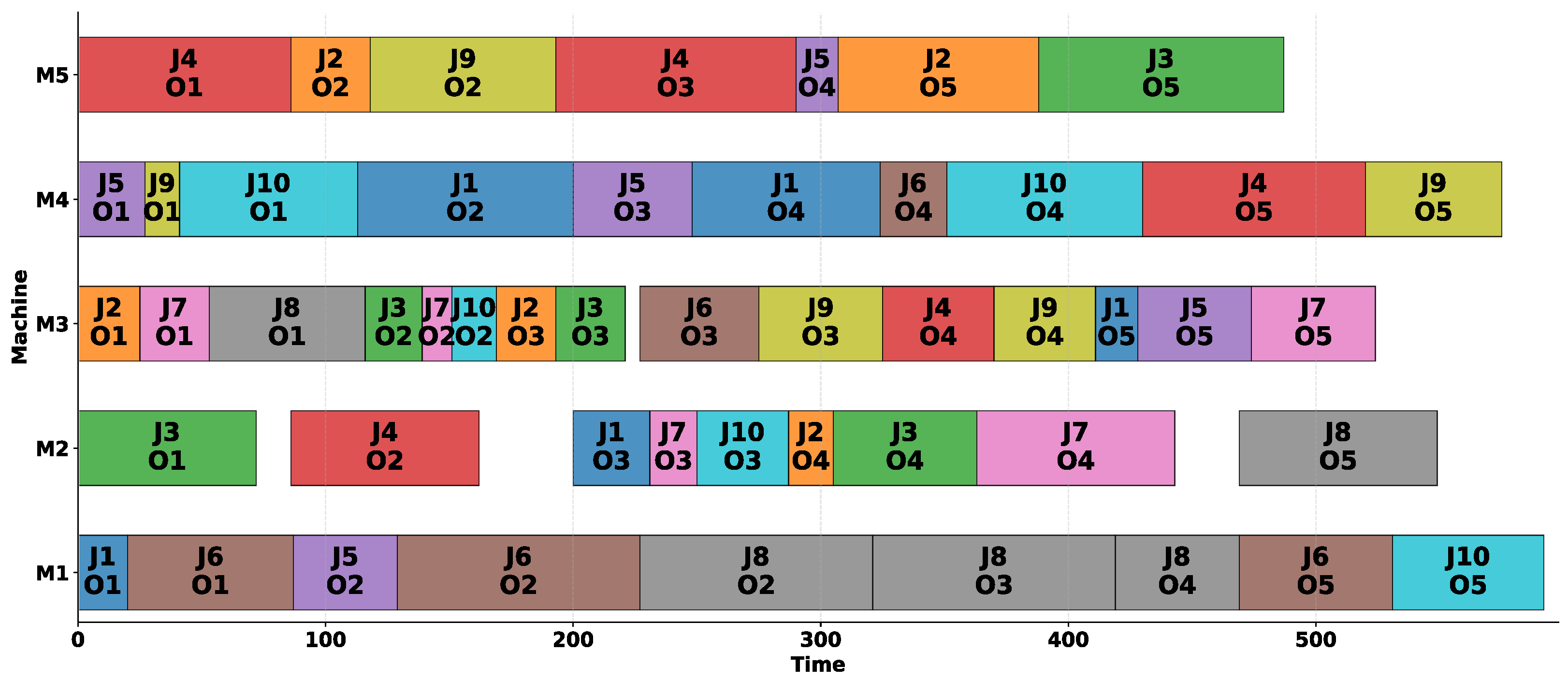
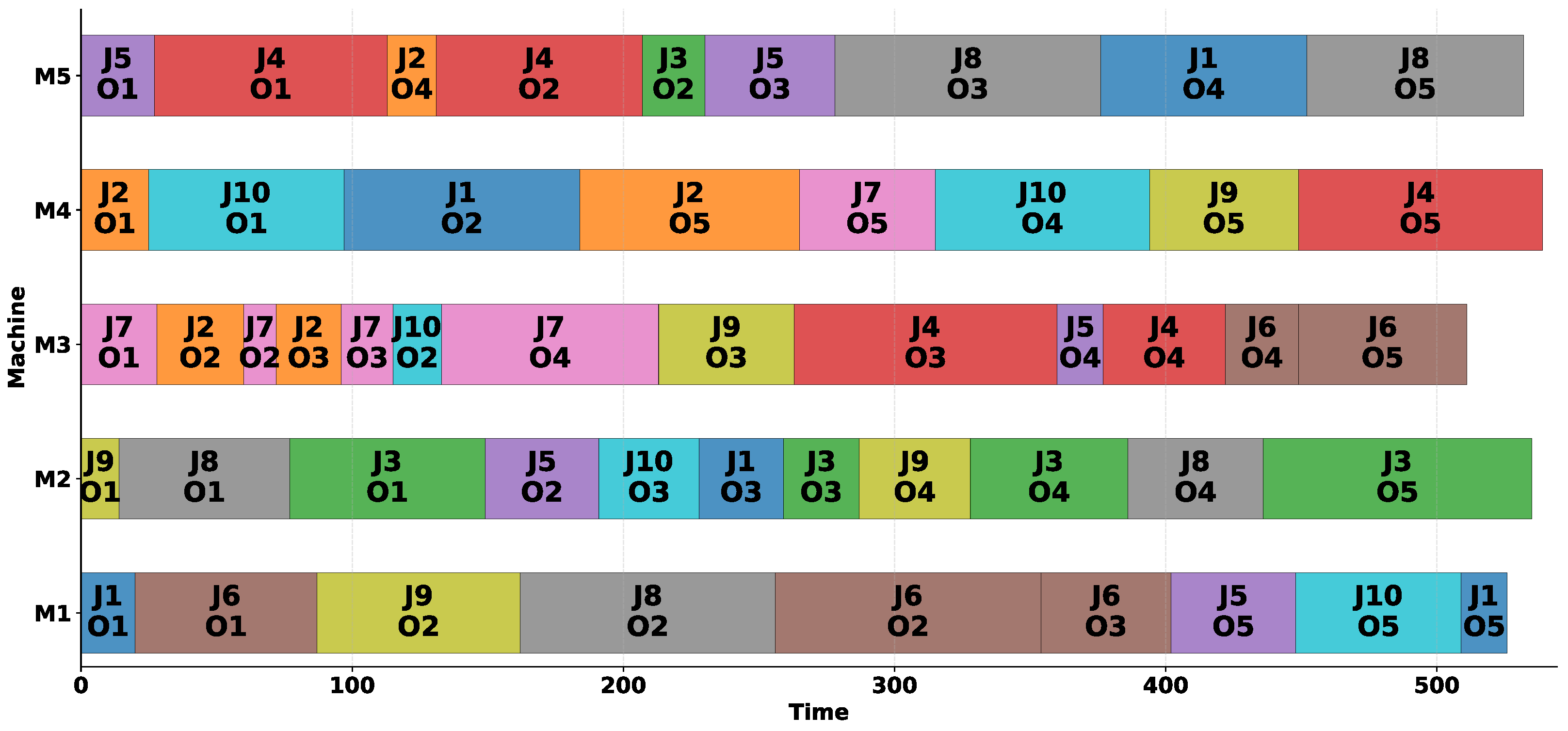
To intuitively demonstrate the scheduling quality, Figure 14 and Figure 15 present Gantt charts for instance la02 from the Hurink dataset, comparing the composite heuristic rule (FIFO + EET, makespan = 592) with the proposed method (makespan = 539, 8.95% improvement). Beyond the quantitative gain, qualitative examination reveals distinct characteristics: The heuristic schedule (Figure 14) exhibits severe idle time concentration, particularly on Machine M5, which remains largely idle from time 300 to 592 (approximately 49% of the makespan). The average machine utilization is only 89.03%, with significant load imbalance across machines. In contrast, the proposed method (Figure 15) generates a more compact schedule with minimal idle gaps. All machines maintain high activity levels throughout the scheduling horizon, achieving 98.08% average utilization. The workload is more evenly distributed, preventing bottlenecks and maximizing temporal parallelism. This visual comparison confirms that GIAN+EAE-PPO not only achieves lower makespan values but also generates more efficient and balanced schedules suitable for practical deployment.

Based on the experimental results across three public datasets, the following conclusions can be drawn: The proposed GIAN + EAE-PPO method achieves a superior balance between scheduling performance and policy stability. Compared to SAC-based methods, it effectively suppresses policy fluctuations and overcomes performance oscillations caused by estimation volatility, as evidenced by compact boxplots and lower mean values. Compared to PPO-based methods, it significantly enhances exploration efficiency in complex solution spaces through the synergistic design of the graph attention encoder and the entropy adaptive exploration mechanism. Consequently, the proposed method demonstrates robust and state-of-the-art performance in solving the Flexible Job Shop Scheduling Problem.

5.5. Robustness Analysis and Boundary Cases

While the average performance metrics demonstrate the superiority of GIAN + EAE-PPO, a comprehensive evaluation requires examining outliers and boundary cases to assess algorithmic robustness. Outlier Identification. We systematically analyzed instances where our method exhibits higher-than-average scheduling gaps.

Table 2. Outlier Analysis—Instances with Highest Gaps.

Dataset	Instance	Scale	UB	Ours	Gap (%)	Best Baseline	Baseline Gap (%)	Relative Rank
Brandimarte	MK10	20 × 15	198	237	19.7	DAN + PPO: 230	16.1	3rd/10
Brandimarte	MK06	10 × 15	58	69	19.0	SAC-amber: 72	24.1	1st/10
Hurink	La(21–25)	15 × 10	841	979	16.4	HGNN + PPO: 959	14.0	2nd/8
Dauzère	16a	20 × 25	2255	2696	19.6	MLP + PPO: 2680	18.8	2nd/8
Dauzère	13a	20 × 25	2260	2696	19.3	DAN + PPO: 2622	16.0	2nd/8
Dauzère	07a	15 × 25	2283	2711	18.7	DAN + PPO: 2643	15.8	3rd/8

summarizes the identified outliers across three datasets.

A critical finding emerges: high scheduling gaps do not necessarily indicate poor algorithmic performance. On instance of MK06 (Gap = 19.0%), our method achieves the best absolute makespan (69) among all compared methods, outperforming the second-best baseline by 4.2%. Similarly, on instances 16a and 13a, where gaps approach 20%, the absolute makespan values remain highly competitive, differing from the best baselines by less than 1%. These results suggest that elevated gaps often reflect inherent instance difficulty rather than algorithmic weakness. Notably, in 4 out of 6 identified outlier cases, our method achieves top-2 rankings. As visualized in Figure 11, Figure 12 and Figure 13, the box plots reveal critical distributional differences across methods. A particularly striking finding is the complete absence of statistical outliers in GIAN + EAE-PPO across all three benchmark datasets. In contrast, several baseline methods exhibit outliers: DAN + PPO shows 1 outliers on Brandimarte, GIN + SAC exhibits 1 outlier on Brandimarte and 1 outlier on Hurink. The traditional heuristic rule (BR) also suffers from 1 outliers on Hurink datasets. This zero-outlier characteristic of our method demonstrates exceptional consistency and effective worst-case control, confirming that the EAE-PPO mechanism successfully maintains stable convergence while avoiding the catastrophic failures occasionally observed in SAC-based approaches.

Cross-scale analysis reveals robust performance across diverse problem sizes. On the Brandimarte dataset, our method handles instances ranging from 10 × 6 to 20 × 15 with an overall gap of 8.51%. On the Hurink dataset, spanning from 10 × 5 to 30 × 10, the overall gap is 9.09%. On the Dauzère dataset, featuring the largest instances (up to 20 × 25), the gap is 9.76%. This consistent performance across scales demonstrates effective generalization. Examination of challenging instances (Table 2) reveals common characteristics: high machine flexibility (>80% of operations processable on multiple machines), unbalanced job–machine ratios (e.g., 10 jobs with 25 machines in Dauzère), and long operation sequences (>20 operations per job), suggesting potential directions for future adaptive mechanisms.

6. Conclusions

In this study, an end-to-end framework integrating a GIAN and an EAE-PPO is proposed to address the FJSP. This approach aims to balance the trade-off between stability and exploration in DRL while overcoming the limitations of traditional GNNs in representing global long-range dependencies. A structured exploration curriculum mechanism based on linear and Lagrange polynomial interpolation is designed, which enables the on-policy framework to achieve exploratory capabilities akin to off-policy learning. Additionally, the GIAN is utilized to enhance state representation, facilitating intelligent scheduling decisions in complex industrial scenarios and promoting the evolution towards Industry 5.0.

Numerical experiments across standard benchmark datasets, including Brandimarte, Hurink, and Dauzère–Pérès, demonstrate the effectiveness and superiority of the proposed method compared to mainstream PPO-based and SAC-based methods. In particular, the proposed framework exhibits superior convergence consistency and robustness when handling large-scale tasks with long operation sequences, effectively mitigating the training oscillation problems often observed in maximum entropy methods.

For future work, we will consider the impact of stochastic disturbances, such as machine failures and dynamic order insertions, on real-time adaptability. Extending the online adaptive capability of the EAE mechanism to dynamically adjust exploration strategies based on environmental feedback is a key direction. Moreover, more refined modeling methods, such as HGNNs, can be explored to capture the complex dynamic relationships between heterogeneous entities like personnel and AGVs, further enhancing the generalization capability in real-world dynamic shop floor environments.