4.1. The Gas Turbine Machine Control via the Proposed Method
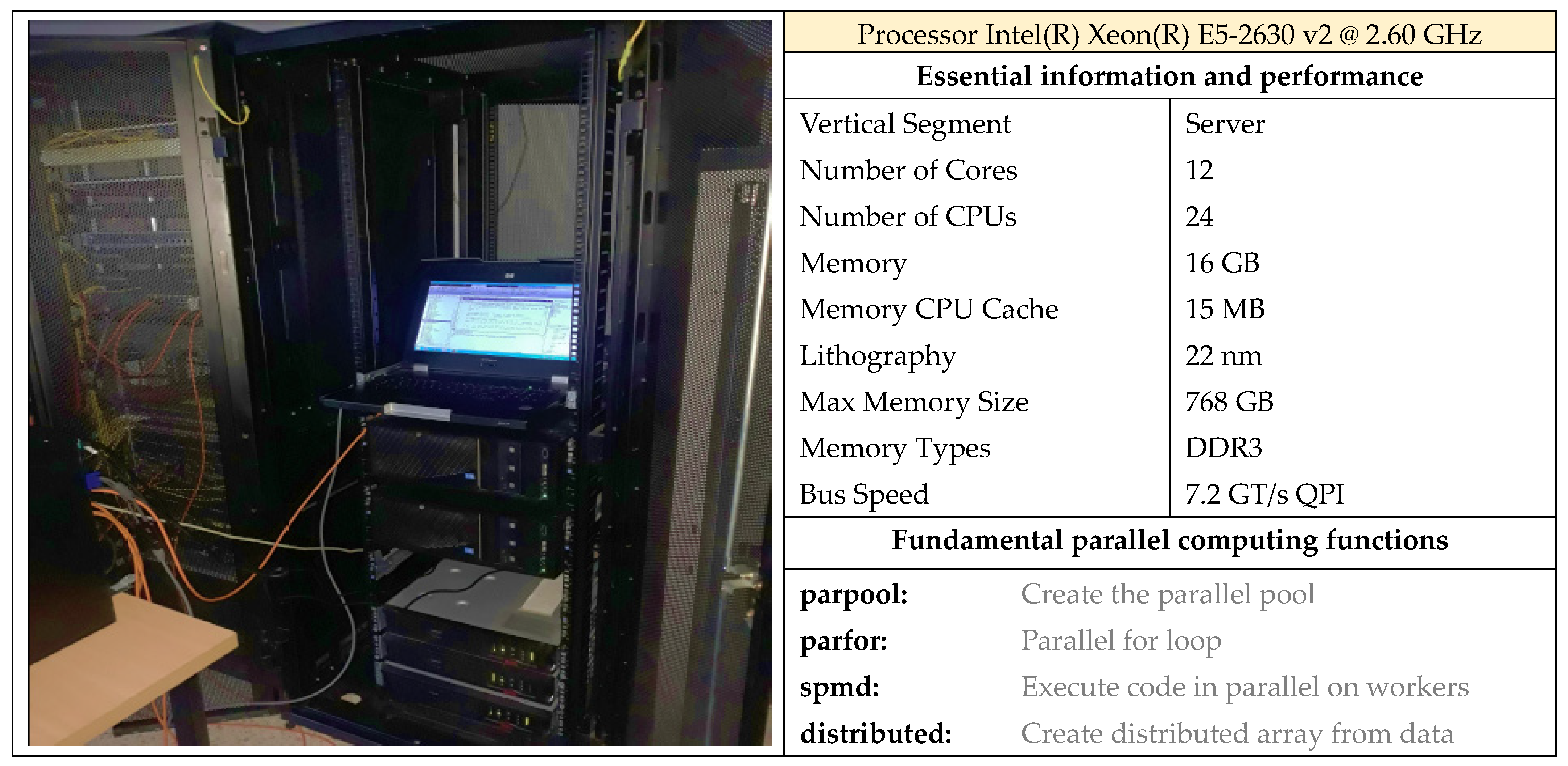
This section studies the GE MS5001P gas turbine at M’SILA power plant (Algeria), selected for its available real-time data. The plant has 22 single-shaft turbines driving the main generators. Each turbine includes an axial compressor, a combustion chamber, and a multi-stage turbine. Rare start-up/shutdown transients are excluded [
29,
30,
31,
32]. Key characteristics of this gas turbine machine are in
Table 1.
The single-shaft industrial gas turbine GE MS5001P is considered to operate in the vicinity of a nominal steady-state condition under ISO ambient conditions. The dynamic model is derived by linearizing the nonlinear thermodynamic equations about a selected equilibrium (trim) point [
34].
Assumptions:
Numerous parameters influence gas turbine dynamics (
Appendix A), with their impact varying according to their role within the main sections of the turbine, namely the compressor, the combustion chamber, and the turbine. In this study, the modeling effort is deliberately restricted to the two principal output variables of the GEMS5001P gas turbine under normal operating conditions: the rotor speed and the exhaust gas temperature. These outputs are directly affected by, and dynamically coupled with, three main variables: the gas control valve (GCV), the axial compressor discharge temperature (TCD), and the axial compressor discharge pressure (PCD) [
28].
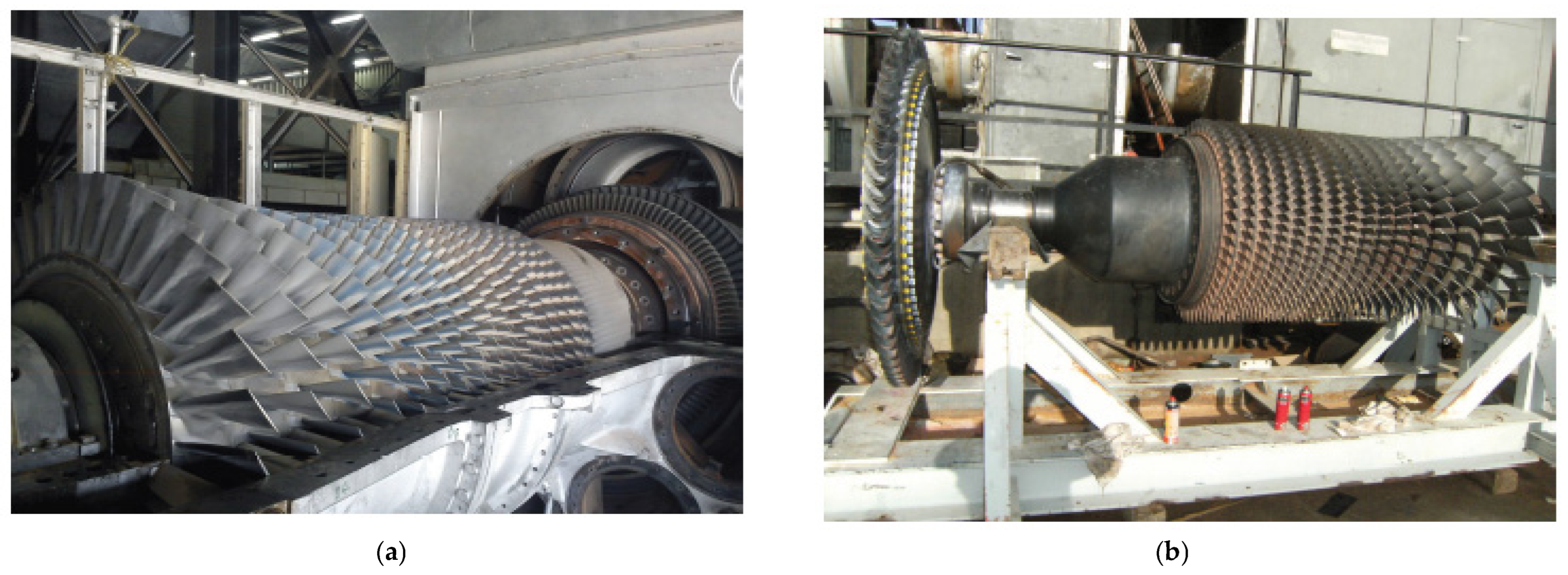
Figure 1. illustrates the axial compressor of the GE 5001P gas turbine and the turbine section of the same system.
The overall dynamics of the gas turbine can be described by a nonlinear multivariable state–space model that captures the coupled mechanical, thermodynamic, and fluid-flow phenomena of the compressor–combustor–turbine assembly. The nonlinear model is expressed as
where
,
, and
. The state vector is defined as
with
is the rotor speed,
and
are the compressor discharge temperature and pressure,
is the turbine inlet temperature,
is the exhaust gas temperature, and
is the shaft torque. These states describe the dominant nonlinear interactions between the rotating shaft dynamics and the thermal processes occurring in the compressor, combustor, and turbine. The input vector is given by
where
denotes the gas control valve position governing the fuel mass flow rate into the combustor, and
is the input compressor discharge temperature, which indirectly affects combustion efficiency and downstream thermal dynamics [
30,
31,
32,
33]. The complex nonlinear model can be written as
where
is the shaft inertia.
,
are the turbine and compressor efficiency factors.
is the fuel mass flow rate (controlled via GCV
).
is the air mass flow rate through the compressor.
,
are the specific heats.
,
,
are gains capturing rotor-compressor coupling, and
is the thermal time constant.
is the steady-state compressor pressure as a function of rotor speed,
is the pressure time constant.
,
representing the effect of fuel flow and compressed air on turbine temperature.
captures the dynamic coupling between rotor speed and exhaust gas temperature,
is exhaust thermal constant.
is a mechanical gain and
is the shaft torque time constant. The measured outputs are selected as
since rotor speed and exhaust gas temperature are the most relevant performance indicators during normal operating conditions.
This is now a completely explicit nonlinear model, including all six states, two inputs, and the outputs. It is suitable for simulation, control design, and linearization. The linear model is obtained by
linearization around a steady operating point . The states’ deviations considered are as follows: the rotor speed
, the compressor discharge temperature
, the compressor discharge pressure
, the turbine inlet temperature
, the exhaust gas temperature
, and the shaft torque
. These states capture the dominant interactions among the compressor, combustor, and turbine, including both thermal and mechanical dynamics. The system is influenced by two independent inputs: the gas control valve
, which modulates the fuel flow into the combustor, and the compressor discharge temperature reference
, which affects the air–fuel mixture and consequently the downstream thermal states. The two measured outputs are the rotor speed and the exhaust gas temperature, denoted as
and
, which are the primary indicators of turbine performance in normal operating conditions [
28,
30].
Finally, the linear model is obtained by linearizing the nonlinear dynamics around a nominal steady-state operating point
, corresponding to normal turbine operation, leading to the deviation model
. The operating point is computed by solving the trimming conditions
using optimization-based methods. The state-space matrices
,
, and
can, in principle, be obtained by evaluating the Jacobians of the nonlinear system
at the nominal operating point
. However, since many of the physical constants and parameters are not known a priori, an identification-based approach is employed to derive an approximate continuous linear model that accurately captures the system dynamics around the operating point [
34].
4.2. Recursive Methods for Continuous Time System Identification
The multivariable continuous time recursive least square (MCTRLS) is an algorithm stated to minimize the criterion
So that the least square estimate is
For adaptive control applications, we are interested in recursive formulation where the parameters are updates continuously on the basis of input output data. Such update may be obtained by defining
Finally, we can write (with some forgetting Factor) this steps in Algorithm 2.
| Algorithm 2 Multivariable Continuous Time Recursive Least Square |
| Step 1: | Input , and form the data matrix | If we define the matrix then |
| Step 2: | | |
| Step 3: | | |
| Step 4: | | |
Linear continuous-time systems can be described in two main ways: the state-space (internal) representation, which captures the system’s dynamics via state variables, and the input-output representation, expressed either as a time-domain differential equation or as an order transfer function in the s-domain. Previously, we reviewed identification methods based on numerical integration, which require measurements of all states and inputs. In contrast, the method presented here relies only on the input sequences and a single output sequence to estimate the continuous-time system parameters.
The trapezoidal rule approximates the integrand
by a linear function over each interval
. Within this interval, the linear approximation—known as a trapezoidal pulse function—can be expressed as follows:
Here,
denotes
. The identification method requires successive integrals of
to estimate the continuous-time system parameters. Accordingly, a set of approximate formulas is used to compute these integrals. Over the interval
, the area under the linear approximation of
equals the standard trapezoidal integral. The recursive formula for the first and second integral of
then can be expressed as follows:
In general, we can express the
integral of
by the following equation
Now, the identification problem can be easily solved by simple applying this equation to the differential equation of continuous-time systems. Consider the MIMO continuous-time system described by
or by
The identification problem now is to estimate the parameters
and
. Integrating both sides of the above equation
times with respect to
over the subinterval
, we obtain
where the differences are
,
and
. The quantities
and
are the
integrals of
and
at the
sampling instant, respectively.
A multivariable continuous-time identification is performed via a trapezoidal integration–based recursive least squares (RLS) scheme as shown in Algorithm 3.
| Algorithm 3 Multivariable Continuous Time Trapezoidal Integral RLS (For a 2nd order MDFD model) |
| 1 | Given: |
| 2 | |
| 3 | |
| 4 | |
| 5 | |
| 6 | %-----Initial Values-----% |
| 7 | ; | % with θ = [D1′;D2′;N1′;N2′] |
| 8 | ; ; | % Covariance matrix |
| 9 | ; ; ; ; | % Initialize integral states |
| 10 | |
| 11 | %-----Data Acquisition-----% |
| 12 | For k = 1:N, ; End % where represents the real system dynamics. |
| 13 | For k = 2:N-1 |
| 14 | %-------Integrations-------% |
| 15 | | % Local trapezoidal integrals |
| 16 | | % Cumulative 1st integral |
| 17 | | % Local 2nd order integrals |
| 18 | | |
| 19 | %-------RLS Algorithm-------% |
| 20 | ; | % Output increment |
| 21 | ; | % Regressor vector |
| 22 | ; | % RLS gain |
| 23 | ; | % Parameter update |
| 24 | ; | % Covariance update |
| 25 | End |
As discussed previously, it is often preferable to identify the parameters of a continuous-time system directly from discrete input-output measurements. The core concept is to integrate the system’s differential equations over each sampling interval, yielding relationships between the sampled input-output data and the unknown model parameters. For instance, consider a state-space representation where the state is assumed measurable and is a white noise process. where , , and . The terms , , are parameter matrices. The objective is to identify the system matrices from sampled input–state data and collected at , for . The sampling period is assumed sufficiently small to preserve the system dynamics. In practice, the identification is complicated by measurement noise.
If we integrate the differential equation in
between the limits
and
, we obtain
and
Exact evaluation of the integrals is infeasible since only noisy samples of
, and
are available. Therefore, the integrals are approximated using sampled data under an assumed model structure. Numerical integration–based identification methods are adopted, assuming a minimal (controllable and observable) system realization. If we choose a trapezoid to approximate the area of a typical panel, then we have the Trapezoidal rule, that is
By using this identification method we see that the discrete-time system obtained is identical to the one calculated by the bilinear z transformation. Clearly, if we have all the state measurements and the input samples, the parameters
and
can be easily estimated by applying the least squares approach
Or in compact form we write
By using the ordinary least square we obtain
whose optimal values is given by
where the matrix
can be approximated by
Now let us implement this identification method using Algorithm 4.
| Algorithm 4 Multivariable Continuous Time Identification (For a Gas Turbine Model) |
| 1 | Given: |
| 2 | | % Sampling period |
| 3 | | % Initial and final time |
| 4 | | % Input and state vectors |
| 5 | | % Parameter matrix |
| 6 | | % Number of samples |
| 7 | | % The overall time grid |
| 8 | | % Initial values |
| 9 | %----- Data Acquisition -----% |
| 10 | For k = 1:N, ; End
% where represents the real system dynamics. |
| 11 | %-------State Space Model by Ordinary Least Squares (OLS) Algorithm-------% |
| 12 | For k = 1:N−1 |
| 13 | ; | % Update time index |
| 14 | ; ; | % Trapezoidal rule for state and input |
| 15 | ; ; | % Increment over ∆t and regression row |
| 16 | ; ; | % Stack regressor matrix and state vector |
| 17 | ; | % Advance time |
| 18 | End |
| 19 | ; | % Batch OLS (offline estimation) |
| 21 | ----------------------------------------------------------------------------------- |
| 22 | In previous code we have seen the identification by the OLS algorithm which requires of providing the data instantaneously, due to such reason we must change the identification scheme to the recursive version. |
| 23 | ----------------------------------------------------------------------------------- |
| 24 | %-------State Space Model by RLS Algorithm-------% |
| 25 | ; ; | % Initial parameter and covariance matrix |
| 26 | For k = 1:N |
| 27 | ; ; | % Time update |
| 28 | ; ; | % Trapezoidal integration |
| 29 | ; ; | % Increment and instantaneous regressor |
| 30 | ; | % RLS gain computation |
| 31 | ; | % Parameter update |
| 32 | ; | % Covariance update |
| 33 | ; ; | % Extract estimated system matrices |
| 34 | End |
The identified model is validated using statistical and performance metrics. The “Akaike Information Criterion” (AIC) and the “Final Prediction Error” (FPE) assess the accuracy–complexity trade-off, the “Root Mean Square Error” (RMSE) measures average prediction error, and “Variance Accounted For” (VAF) indicates how well the model reproduces output dynamics. Together, these indices ensure both accuracy and robustness. The AIC for an estimated model: where is the loss function, is the number of estimated parameters and is the number of samples in the estimation data set. The Akaike’s FPE is defined by . The normalized , is given by the expression: . The “variance accounting for” is defined as follows: . The optimal system order corresponds to the minima of AIC, FPE, RMSE and the maximum of VAF.
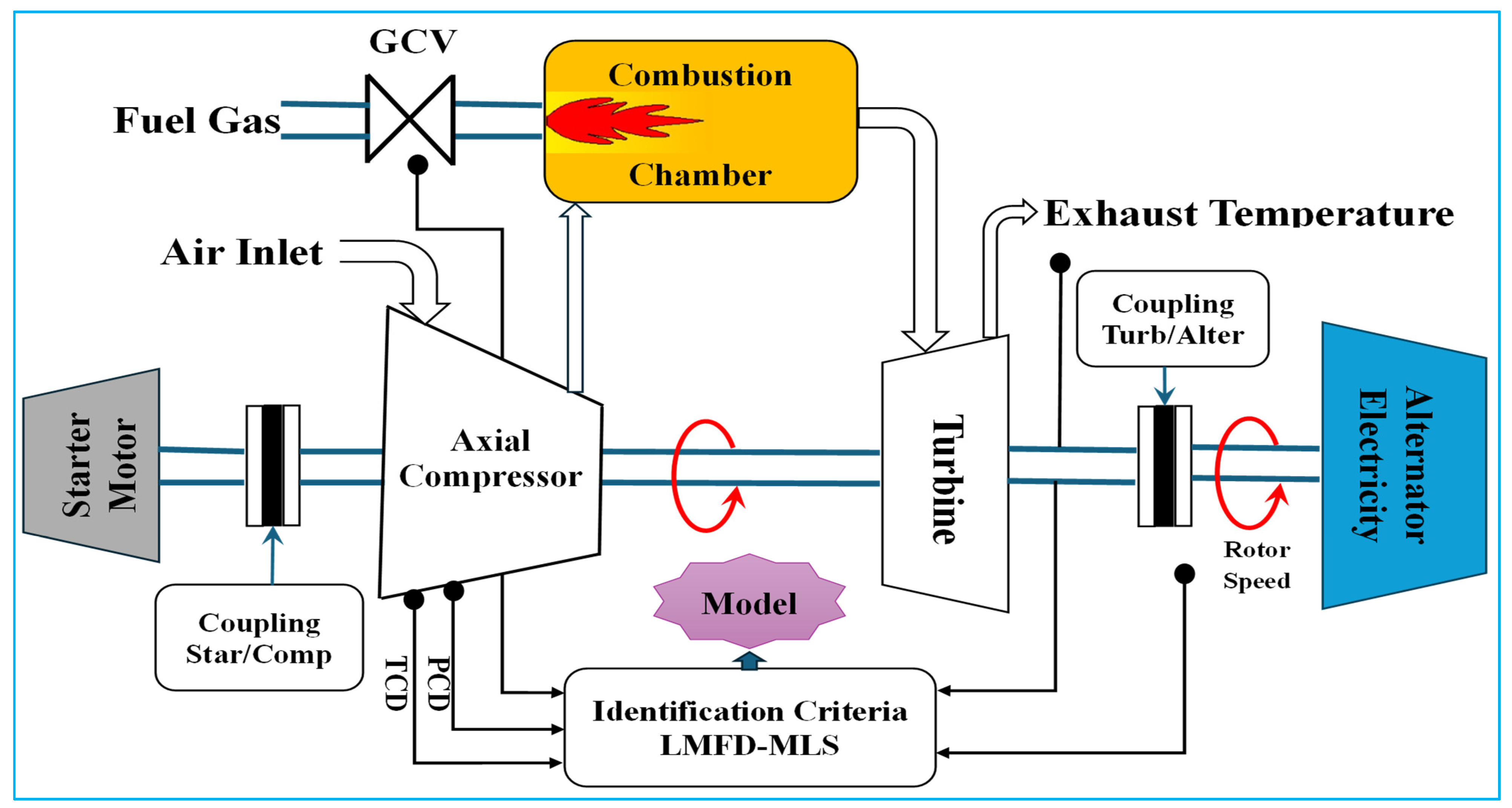
A schematic diagram for turbine identification is shown in
Figure 2, illustrating the system inputs and outputs, the main components (axial compressor, combustion chamber, and turbine), and the electrical alternator as the load [
31].
The following state-space representation models the gas turbine dynamics
Gas control valve (fuel flow command);
Compressor discharge temperature reference;
Rotor speed;
Exhaust gas temperature.
Physical Interpretation: Rotor speed is governed by shaft torque and turbine temperature, while compressor discharge temperature and pressure are strongly coupled, and exhaust temperature reflects combustion and turbine expansion dynamics. Shaft torque provides the link between thermal and mechanical subsystems. The GCV influences fuel flow, turbine temperature, torque, and speed, whereas the TCD reference regulates compressor and exhaust thermal states. Within this context, block controllability represents the ability to regulate these coupled mechanical–thermal subsystems through the available actuators. The identification results are evaluated by comparing the model-predicted outputs with the measured data.
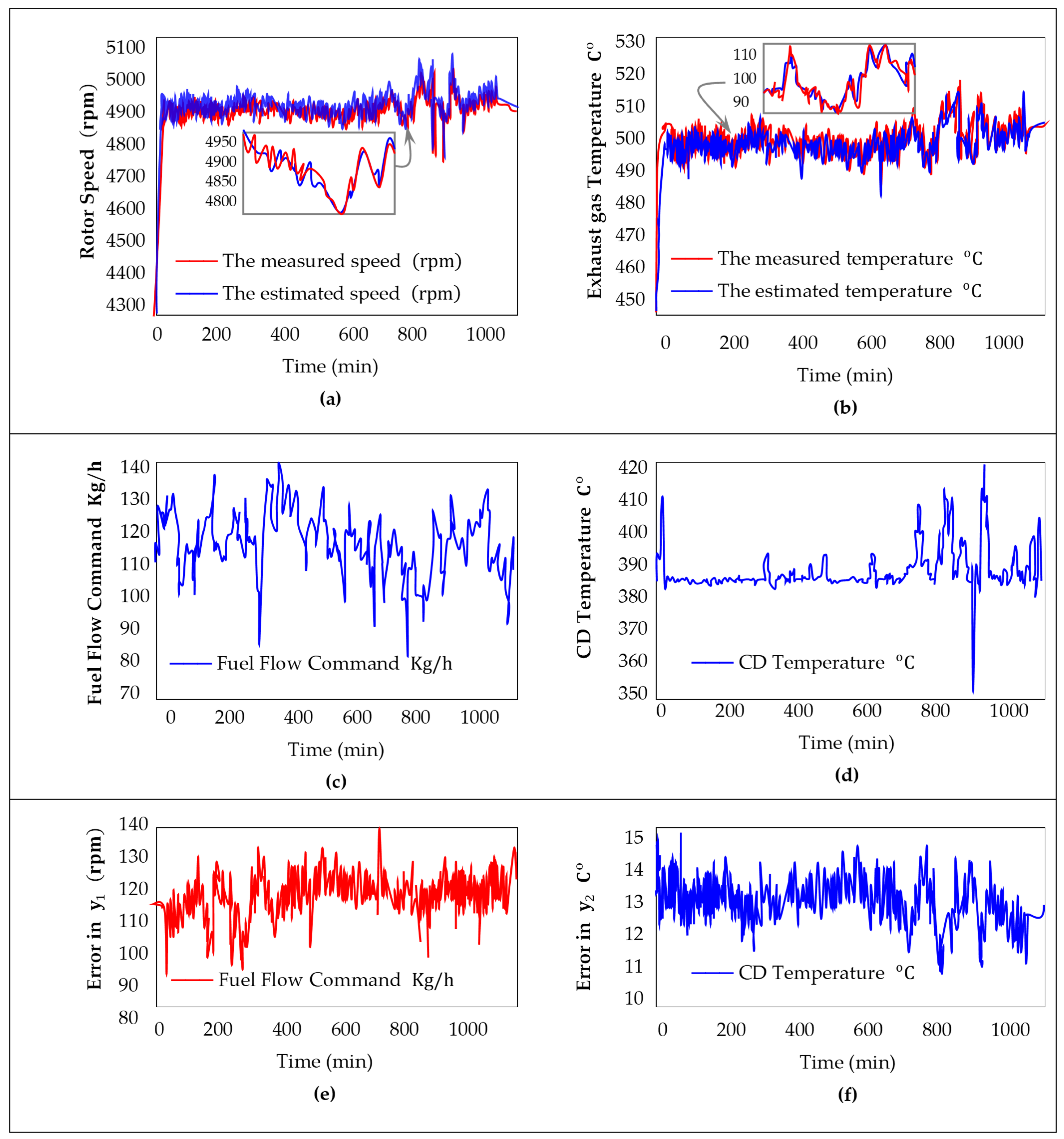
Figure 3 shows the temporal evolution of the input signals, the resulting state trajectories, and the corresponding outputs.
Figure 3 illustrates the temporal evolution of the system inputs, states, and outputs, together with the associated modeling errors. Specifically,
Figure 3a compares the measured and estimated rotor speed
, while
Figure 3b presents the measured and estimated exhaust gas temperature
, showing a close agreement in both cases. The applied fuel flow command is depicted in
Figure 3c, and the corresponding combustion chamber (TCD) temperature response is shown in
Figure 3d. The modeling accuracy is further assessed through the error signals, defined as the difference between measured and estimated outputs, where
Figure 3e shows the error in rotor speed
and
Figure 3f shows the error in exhaust gas temperature
. As observed, the errors remain small over the entire operating range, indicating that the identified model accurately captures the system dynamics and provides a reliable basis for control design.
Table 2 shown below clarifies the change in the orders
until the best one is reached. From the results of this table, it can be concluded that the best model, which fits the minima of AICs, FPEs, RMSEs, the maximum of VAF validation criteria, and the minimum loss function without pole/zero cancelation (left coprime), is the model of order
with number of blocks
.
4.3. Supervisory Control of the Gas Turbine Machine
In order to fulfill the main objective of this paper, the proposed algorithm is implemented on the studied system in accordance with the previously described steps.
- ✓
The ratio equals to , it is an integer.
- ✓
The block controllability matrix is satisfied as (full rank).
- ✓
The transformation matrix is calculated by Equations (31)–(33).
- ✓
Construct the desired right block roots such that is nonsingular.
- ✓
Find the matrix coefficient and by Equations (34) and (35).
- ✓
The feedback gain matrix is calculated based on (32) or (48).
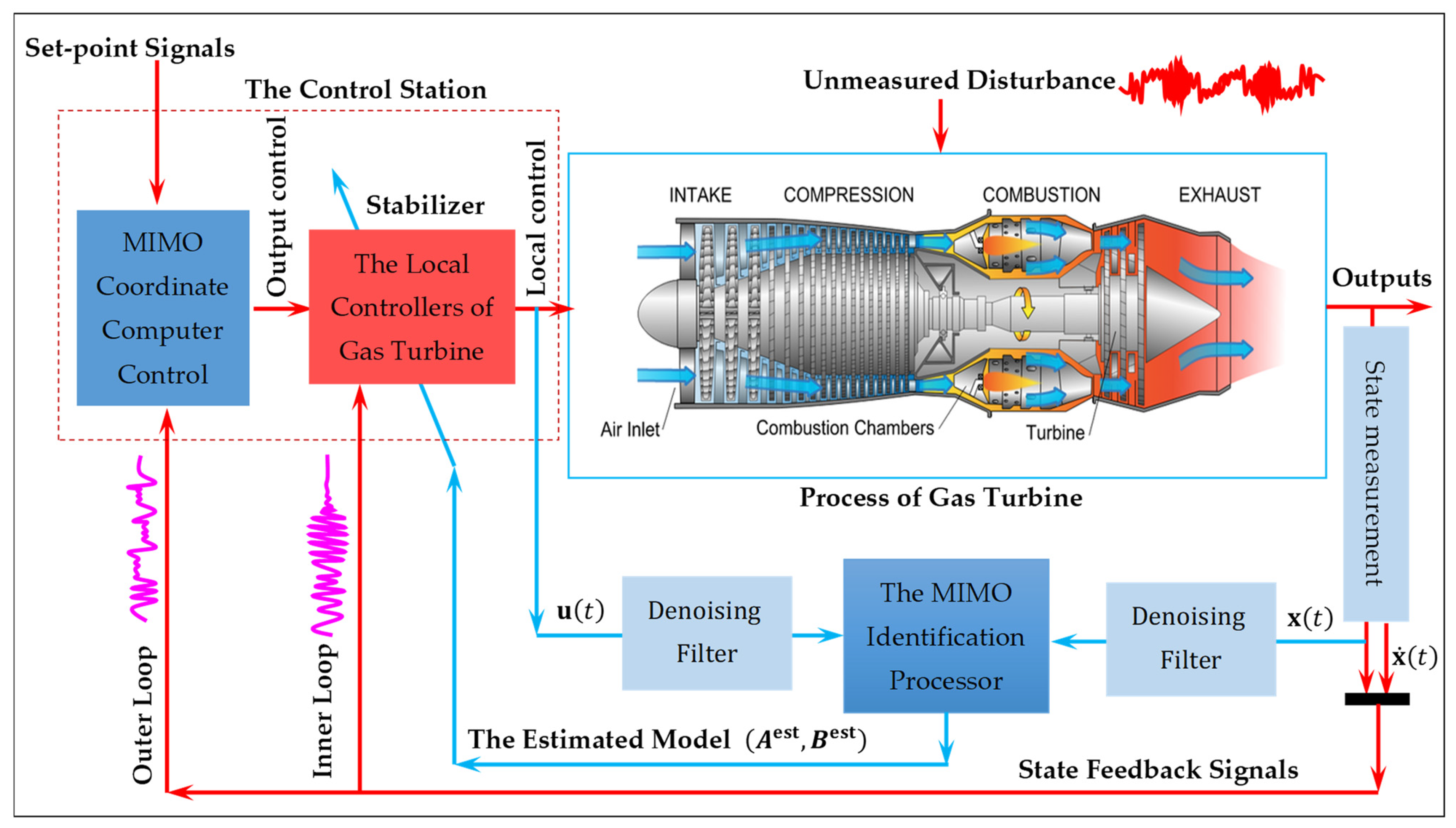
The overall supervisory control architecture, including the reference adjustment mechanism, is illustrated in
Figure 4.
In recent years, various control strategies have been proposed for multivariable gas turbine systems, involving trade-offs between performance, robustness, and computational complexity. Robust and adaptive methods such as H∞ and sliding mode control effectively handle uncertainties and disturbances but often increase controller complexity and tuning sensitivity [
29,
30]. Model Predictive Control (MPC) provides systematic constraint handling and multi-objective optimization, yet its computational burden can limit real-time implementation for fast dynamics [
32]. Matrix-based and linear algebraic approaches, including generalized eigenstructure assignment and block polynomial methods [
27,
36], are closely related to the present work through closed-loop pole assignment and structured state feedback, but typically assume full state availability or suffer from higher algebraic complexity in MIMO extensions. Observer-based schemes address state unavailability at the cost of added dynamics and noise sensitivity [
37,
38].
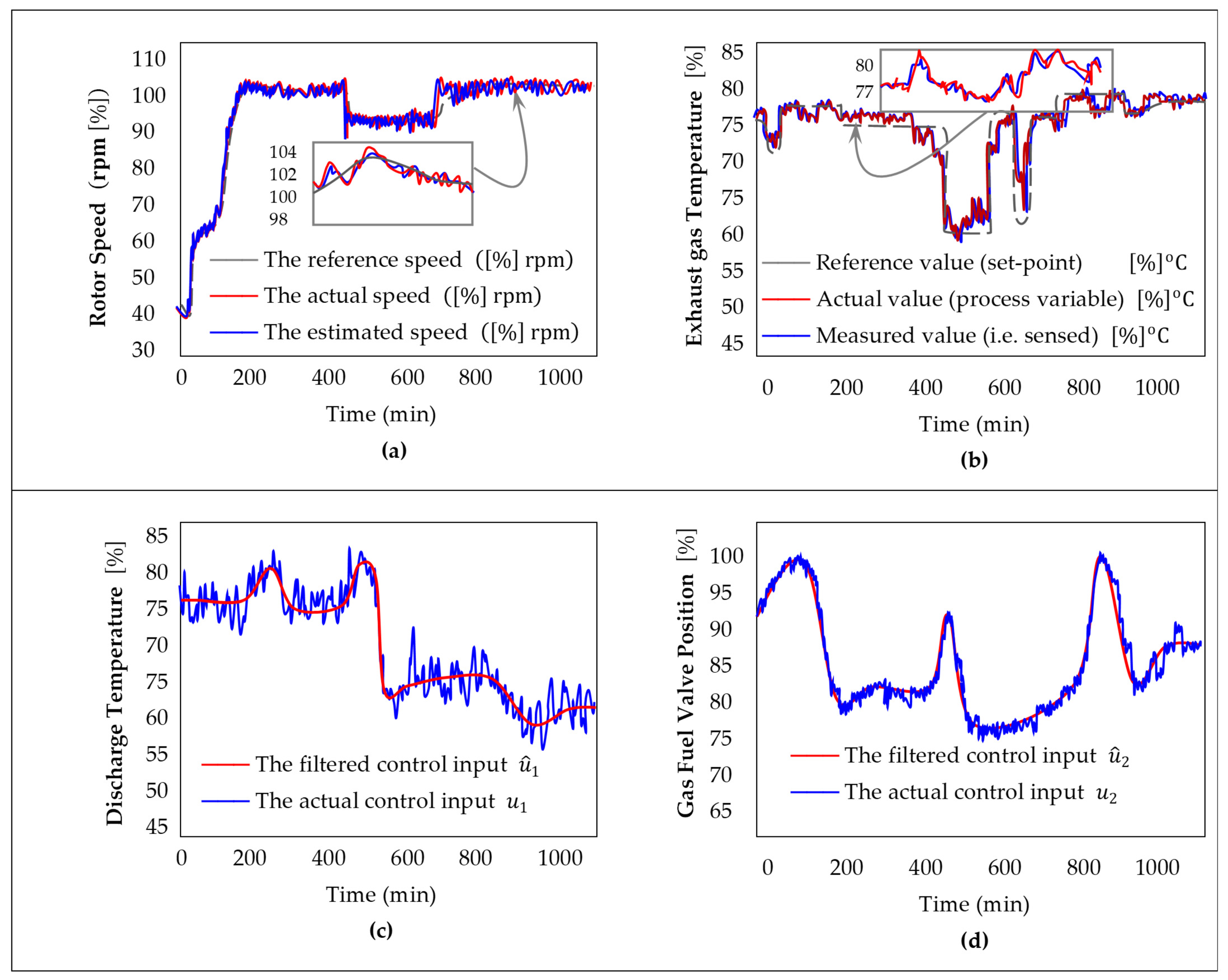
Figure 5 illustrates the dynamic response of the system variables and control inputs. Subplots (a) and (b) show the rotor speed and exhaust gas temperature, respectively, comparing the reference values (setpoints), actual values (process variables), and measured values obtained from sensors. Subplots (c) and (d) present the filtered control inputs alongside the actual control signals, demonstrating the effectiveness of the control strategy in tracking the references and maintaining system stability.
The proposed state-derivative feedback leverages the time derivatives of key mechanical and thermal states to enhance closed-loop performance. By incorporating derivative information, the controller improves damping, reduces overshoot, and accelerates transient response, particularly for rotor speed and shaft torque, which exhibit faster dynamics. In practical implementations, since direct measurement of state derivatives is often infeasible due to sensor limitations and noise sensitivity, the proposed approach relies on estimated derivatives obtained through adaptive filtering techniques that ensure accurate estimation while attenuating measurement noise. Compared to conventional state-feedback approaches, this method achieves superior stability and robustness while maintaining a low computational burden, making it well-suited for real-time control of industrial gas turbines. To demonstrate its effectiveness and advantages, a comparative study (
Table 3) is conducted with classical and recent control strategies, including classical pole placement with stable eigenvalue assignment [
39], discrete time linear quadratic regulator (DLQR) based on minimizing energy criteria [
35], eigenstructure assignment with separate placement of eigenvalues and eigenvectors [
36], stabilizing linear multivariable gas turbine model via sliding mode control [
34], and the proposed linear algebraic state and state-derivative feedback method based on matrix polynomial theory, which simplifies implementation by directly leveraging measurable derivatives and ensures competitive pole placement capabilities.
The table compares the feedback gain norms (,,) for different control methods applied to the gas turbine system. The proposed method and DLQR exhibit relatively low gain magnitudes, indicating moderate control effort and less aggressive feedback, while linear sliding mode shows the highest norms, reflecting stronger control action. Classical pole placement and Eigen-Structure Assignment lie in between, with Eigen-S having slightly higher norms due to the complexity of eigenvector shaping. Overall, the proposed state-derivative feedback achieves a good balance between performance and control effort.
Let
,
and
be the
eigenvalue, right and left eigenvectors of
, respectively, and let
be the
eigenvalue of
(
i = 1, 2, …,
n). Then, the eigenvalue sensitivity is defined as
. The individual relative change in eigenvalues is
for
i = 1, 2, …,
n. Let
be the set of eigenvalues of an
matrix denoted by
and assuming that all the eigenvalues are stable
and have been arbitrarily assigned to guarantee performance. The three robust stability measures are defined by the following:
where
denotes the smallest singular value, and
in such a manner:
, the matrix
is the diagonal form of
, and
[
7].
The sensitivity of the closed-loop eigenvalues with respect to perturbations in the system matrix is presented in
Table 4, where the proposed method consistently exhibits lower sensitivity values compared to the other methods.
As shown in
Table 5, the proposed method exhibits the smallest relative eigenvalue variations under perturbations while achieving the largest stability margins
,
, and
, confirming its superior robustness performance.
From
Table 4 and
Table 5, it is observed that the proposed method yields significantly lower eigenvalue sensitivities
and smaller relative variations
under perturbations compared with the classical and recent control strategies. Moreover, the associated stability measures
–
attain their highest values for the proposed approach, indicating improved robustness margins and enhanced tolerance to modeling uncertainties.
Table 6 compares the settling time (
) and maximum peak (
) of each state for different control methods.
The proposed method achieves the fastest settling times and the lowest overshoots across all states, indicating superior transient response and damping. While DLQR and ES-assignment also show moderate improvements over pole placement, linear sliding mode reduces overshoot for some states but does not consistently outperform the proposed approach. Overall, the results highlight the effectiveness of the proposed state-derivative feedback in improving both speed of response and peak suppression.
Table 7 summarizes a qualitative comparison of the considered control methods in terms of gain norm, time-domain specifications, robust stability, and robust performance.
The results of the feedback gain matrix
, obtained by applying all the steps of the proposed state-derivative feedback algorithm, are compared with other control methods, including pole placement, DLQR, Eigen-Structure Assignment, and linear sliding mode. The comparison, summarized in
Table 7, is performed under the same conditions, including identical initial state values, desired pole locations, and a consistent level of injected disturbances. The qualitative evaluation considers key criteria such as norms, time specifications, robust stability measures (
,
,
,
), and robust performance
, highlighting the relative advantages of each method.