An Integrated Control Strategy for Trajectory Tracking of a Crane-Suspended Load

Abstract

With the advancement of intelligent technologies, industrial production systems are being profoundly transformed by artificial intelligence algorithms. To address persistent challenges, such as cargo swing and low operational efficiency during the lifting processes of all-terrain cranes, this research investigates an intelligent control algorithm designed for swing suppression and high-stability payload trajectory control. Firstly, a nonlinear dynamic model of the crane system was derived using the Euler–Lagrange formulation based on a simplified three-dimensional representation. A linear time-varying model predictive control (LTV-MPC) strategy was then designed to incorporate real-time feedback during luffing and slewing motions to monitor the payload’s swing state. On this basis, the controller predicts the desired trajectory and applies negative feedback to adjust the control input, thereby steering the system toward the optimal trajectory and aligning it with the target path. Secondly, a comparative analysis was conducted among four scenarios: the natural swing state of the payload and three control strategies—LTV-MPC, sliding mode control (SMC), and PID control—under both single-input and dual-input conditions. Finally, an experimental platform was established, employing the YOLOv12 algorithm for real-time detection and trajectory tracking of the suspended payload. The experimental results validate the effectiveness of LTV-MPC in suppressing cargo swing. Under single-input control, LTV-MPC achieved the best performance in both stabilization time (3.05 s for luffing condition one and 1.15 s for luffing condition two) and steady-state error (0.003–0.007°). The swing angle, θ₁, was reduced by 91.9%, 54.2%, and 59.3% compared to the natural swing state, SMC, and PID, respectively. In dual-input control, LTV-MPC attained a steady-state error of only 0.0008° under “luffing condition two,” while during slewing operations, it also outperformed SMC and PID in both settling time (26.05 s) and precision (0.008°).

1. Introduction

One of the key factors restricting the operational efficiency of cranes is the payload oscillation during hoisting operations with wire–rope systems, which is induced by rope flexibility and acceleration-induced loads, thus preventing smooth and rapid cargo placement [1]. Given the potential hazards and uncertainties associated with manual operation, efficient control methods need to be designed to enhance the control performance of boom crane systems and effectively suppress payload swing—a challenge that is difficult to overcome even for skilled operators [2]. Previous studies have extensively examined crane systems and payload swing (oscillation) control from various perspectives, with notable findings. In 2019, Tayfun and Soyguder [3] employed classical PID control, fuzzy logic control, and a PID-type fuzzy adaptive controller to regulate the system. In the same year, Dong-Hoon Lee [4] et al. investigated methods for suppressing unexpected vertical vibration in the load, applying several control strategies, including PID control, sliding mode control, and feedback linearization. In 2020, Charles [5] et al. represented the essential nonlinear dynamics of crane systems using a state-space fuzzy model with a compact rule base. In 2021, Christofer Bernardo [6] et al. adopted fuzzy intelligent control for load anti-sway, combined with a classic proportional–derivative (PD) controller tuned via the Ziegler–Nichols method for trolley lateral positioning. Johan [7] et al. derived hanging load dynamics and associated crane kinematics to develop a two-degrees-of-freedom anti-swing controller. Similarly, Die Hu [8] et al. established a dynamic model for a dual-vessel crane system based on the Lagrangian formulation, proposing a controller capable of achieving precise dual-boom positioning while effectively eliminating payload swing. Luo Kai [9] et al. numerically solved the nonlinear deformation displacement at the boom tip using differential equations and coordinate transformation. Subsequently, they proposed a hoisting-luffing coordination strategy based on a preset luffing cylinder extension length via a stepwise progressive approach. In 2022, Tian Gao [10] et al. described frequency analyses of double-pendulum swing and twisting for eccentric loads. Huaitao Shi [11] et al. proposed a novel nonlinear coupled tracking and anti-sway controller, which ensures stable trolley startup and operation by incorporating a smooth reference trajectory. In 2023, Bilgin and Melek [12] designed an additional telescopic boom for anti-sway control, employing a Particle Swarm Optimization Proportional–Derivative–Second Derivative (PSO-PDD²) control system. Fan Bo [13] et al. developed a novel control strategy based on load-energy coupling by analyzing the coupling relationships among various state variables of the crane, achieving both system positioning and elimination of residual payload swing. Sun Mingxiao [14] et al. proposed a PD-based trajectory tracking strategy that accounts for hoisting-length changes. In addressing the limitations of traditional anti-swing control algorithms in tackling ship-mounted crane operations—specifically, the neglect of coupling between rope length variation and swing angle—Yu [15] et al. established a three-dimensional dynamic mathematical model of an overhead crane and investigated the dynamic characteristics of the swing angle. Their methodology provides a valuable reference for related research. Based on nonlinear dynamic modeling of a crane, Shenhao Tong [16] et al. designed a novel variable-structure controller by partitioning the nonlinear system into two subsystems containing displacement and swing angle information. Based on the geometric parameters of a revolving offshore crane vessel, Dapeng Zhang [17] et al. developed a corresponding marine crane model and investigated the motion responses of the suspended payload under various wave conditions. In 2024, Li Dong [18] et al. proposed an adaptive coupled tracking and anti-swing control strategy, designing a controller for adaptive trajectory tracking. Wang Hongdu [19] et al. developed an adaptive fuzzy disturbance observer (FDO)-based control scheme to suppress the swing of a mooring–heavy lift crane (HLC)–cargo system under wave disturbances. Segura [20] et al. designed a novel robust observer-based proportionally retarded controller for perturbed two-dimensional crane systems, accounting for variable rope length. Tom Kusznir [21] et al. proposed a novel nonlinear model predictive control (NMPC) approach to control an underactuated overhead crane system. In the same year, Jingzheng Lin [22] et al. proposed a novel model predictive control (MPC) method that successfully accounted for constraints on both system inputs and outputs while maintaining satisfactory control performance even under persistent ship roll and heave disturbances. In 2025, Abut [23] applied two distinct control methods to the system; the designed control algorithms aim to stabilize the pendulum arms in an upright position and drive the trolley to its equilibrium point.

Based on the existing research foundation, this study introduces a modified model predictive control (MPC) strategy by incorporating linear time-varying inputs, referred to as LTV-MPC. This approach is designed for trajectory tracking and swing prediction of the suspended load in an all-terrain crane system. Simulation comparisons were conducted under identical operating conditions against the natural swing state, SMC, and conventional PID control. The results confirm that the proposed LTV-MPC method effectively suppresses payload swing during both luffing and slewing motions.

2. Selection of Predictive Models

MPC is a model-based optimization strategy that solves an optimal control problem in a finite time domain at each sampling instant. Through a feedback mechanism, the current control input is determined and adjusted via negative feedback based on prediction results, thereby achieving optimal control. MPC explicitly accommodates state and input constraints in multivariable systems while demonstrating superior trajectory tracking performance and robustness. The all-terrain crane represents a typical underactuated system, where the number of degrees of freedom exceeds the number of independent control inputs. Significant coupling exists among its state variables, complicating the control design. To facilitate research, the underactuated system is simplified into a two-input–two-output (TITO) system: the acceleration and hoisting speeds serve as the two control inputs, while the swing angles, θ₁ and θ₂, in the luffing and slewing motions constitute the two control outputs. Both state constraints (swing angle limits) and input constraints (actuator physical limitations) are imposed. Based on a small-angle linearized model derived from calculations, either LTV-MPC or linear time-invariant MPC (LTI-MPC) may be considered. However, during luffing and slewing operations, system parameters such as rope length, l, and boom angle, α, vary over time, resulting in a time-varying system. To address this time-varying nature, LTV-MPC is employed. At each sampling instant, the system model is updated according to the current l and α, and the optimization problems are subsequently solved.

3. Mathematical Model

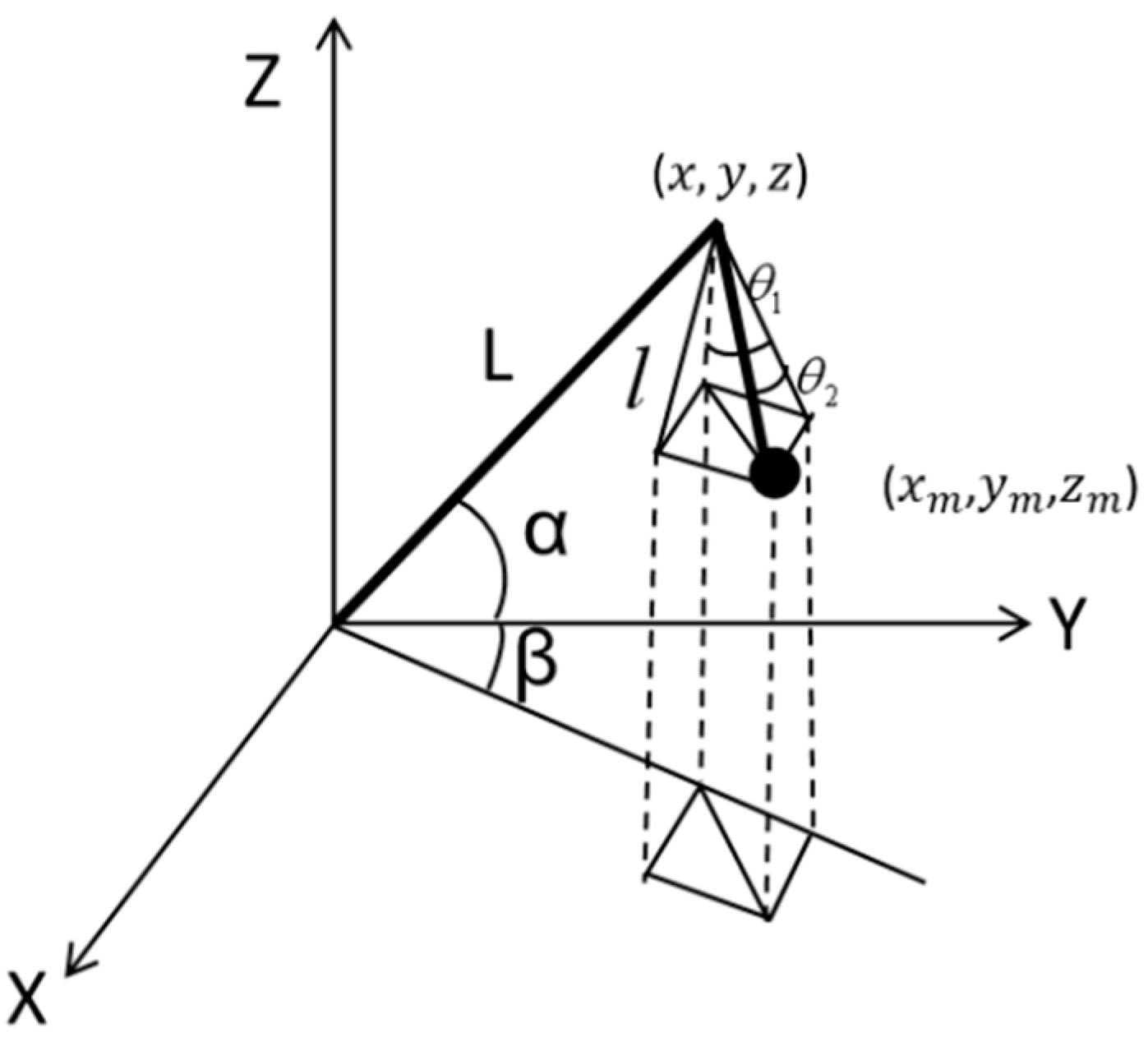
When studying the motion of all-terrain cranes during luffing–hoisting and slewing operations, a simplified dynamic model is established using the Euler–Lagrange method [24]. The following modeling simplifications are adopted: the super-lift device is neglected; the telescopic boom is idealized as a uniform straight beam; and the base is fixed at the coordinate origin. The payload is modeled as a point mass suspended from the boom tip via an inextensible rope. Luffing motion is driven by the luffing cylinder, slewing motion is provided by a slewing mechanism, and hoisting motion is controlled by a mechanism that adjusts the rope length between the boom tip and the payload. Let $\left(x,y,z\right)$ denote the coordinates of the boom tip, and $(x_m,y_m,z_m)$ represent the coordinates of the payload. Define ${\theta }_1$ as the swing angle of the rope in the luffing direction relative to the vertical and ${\theta }_2$ as the swing angle in the slewing direction relative to the vertical. The angle between the boom and the horizontal plane is denoted by α, while β represents the slewing angle relative to the vertical plane. The boom length is denoted by L and the rope length by l.

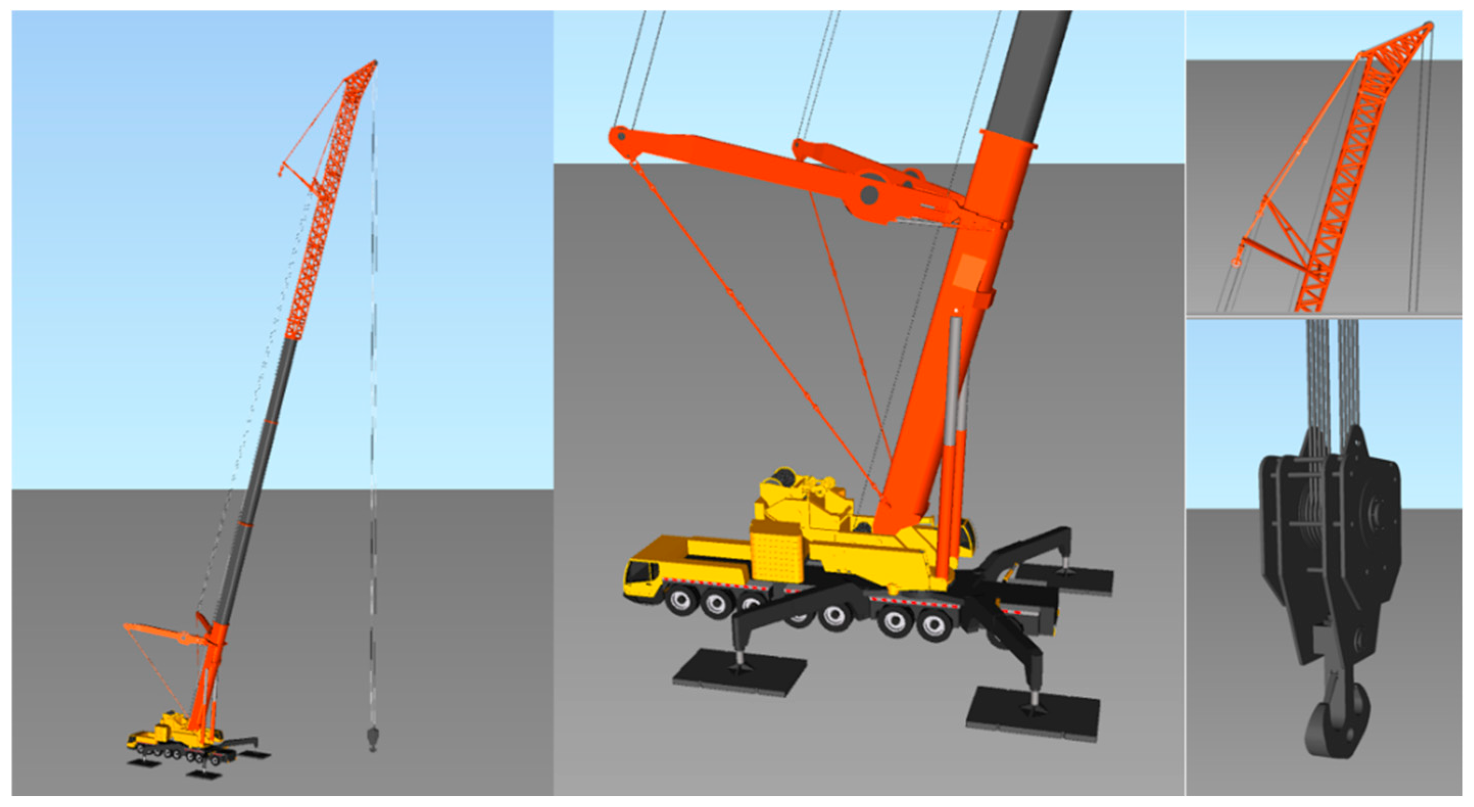
The actual all-terrain crane and its simplified three-dimensional dynamic model are illustrated in Figure 1 and Figure 2, respectively.

The position of the boom tip and the position of the load at any point in inertial space can be expressed as Equations (1) and (2):

$$\left\{\begin{array}{c}x=L\mathit{cos}\alpha \mathit{sin}\beta \\ y=L\mathit{cos}\alpha \mathit{cos}\beta \\ z=L\mathit{sin}\alpha \end{array}\right.$$

(1)

$$\left\{\begin{array}{c}{x}_m=x+l\mathit{sin}{\theta }_1\mathit{cos}{\theta }_2\mathit{sin}\beta +l\mathit{sin}{\theta }_2\mathit{cos}\beta \\ y_m=y+l\mathit{sin}{\theta }_1\mathit{cos}{\theta }_2\mathit{cos}\beta -l\mathit{sin}{\theta }_2\mathit{sin}\beta \\ z_m=z-l\mathit{cos}{\theta }_1\mathit{cos}{\theta }_2\end{array}\right.$$

(2)

The velocity equations of the payload are given in Equations (3)–(5):

$$\begin{array}{l}\begin{array}{c}{\displaystyle \frac{d{x}_m}{dt}}=l{\dot{\theta }}_{2}cos\beta cos{\theta }_2-l\dot{\beta }sin\beta sin{\theta }_2\end{array}\\ +L\stackrel{•}{\beta }\mathit{cos}\alpha cos\beta -L\dot{\alpha }sin\alpha sin\beta \\ +l{\stackrel{•}{\theta }}_{1}sin\beta \mathit{cos}{\theta }_1\mathit{cos}{\theta }_2-l{\stackrel{•}{\theta }}_2\mathit{sin}{\theta }_1\mathit{sin}\beta \mathit{sin}{\theta }_2\\ +l\stackrel{•}{\beta }cos\beta \mathit{sin}{\theta }_1\mathit{cos}{\theta }_2\end{array}$$

(3)

$$\begin{array}{l}\begin{array}{c}{\displaystyle \frac{d{y}_m}{dt}}=l{\stackrel{•}{\theta }}_1\mathit{cos}\beta \mathit{cos}{\theta }_1\mathit{cos}{\theta }_2-l{\stackrel{•}{\theta }}_2\mathit{sin}\beta \mathit{cos}{\theta }_2\end{array}\\ -L\stackrel{•}{\beta }cos\alpha \mathit{sin}\beta -l\stackrel{•}{\beta }cos\beta sin{\theta }_2\\ -L\stackrel{•}{\alpha }\mathit{sin}\alpha \mathit{cos}\beta -l\stackrel{•}{\beta }sin\beta \mathit{sin}{\theta }_1\mathit{cos}{\theta }_2\\ -l{\stackrel{•}{\theta }}_{2}cos\beta \mathit{sin}{\theta }_1\mathit{sin}{\theta }_2\end{array}$$

(4)

$$\begin{array}{c}{\displaystyle \frac{d{z}_m}{dt}}=L\stackrel{•}{\alpha }\mathit{cos}\alpha +l{\stackrel{•}{\theta }}_1\mathit{sin}{\theta }_1\mathit{cos}{\theta }_2+l{\stackrel{•}{\theta }}_2\mathit{cos}{\theta }_1\mathit{sin}{\theta }_2\end{array}$$

(5)

The kinetic energy, T, and potential energy, V, of the load are given by Equations (6) and (7), respectively.

$$T=0.5m(({\displaystyle \frac{d{x}_m}{dt}}{)}^2+({\displaystyle \frac{d{y}_m}{dt}}{)}^2+({\displaystyle \frac{d{z}_m}{dt}}{)}^2)$$

(6)

$$V=mg(L\mathit{sin}\alpha -l\mathit{cos}{\theta }_1\mathit{cos}{\theta }_2)$$

(7)

The Lagrangian operator, L, is defined by Equations (8) and (9).

$$L=T-V$$

(8)

$${\displaystyle \frac{d}{dt}}({\displaystyle \frac{\partial L}{\partial \stackrel{•}{q_i}}})-{\displaystyle \frac{\partial L}{\partial q_i}}=Q_{{\theta }_i}(i=\mathrm{1,2}\dots \dots )$$

(9)

In Equations (8) and (9), L denotes the Lagrangian operator of the system, whose value equals the difference between kinetic energy and potential energy; $q_i$ represents the generalized coordinate of the system, $Q_{{\theta }_i}$ signifies the generalized force, and $i$ indicates the number of degrees of freedom of the particle system. Selecting ${\theta }_1$ and ${\theta }_2$ as the generalized coordinates leads to Equation (10).

$$\begin{array}{c}{Q}_1={\displaystyle \frac{d}{dt}}\left({\displaystyle \frac{\partial L}{\partial \dot{{\theta }_1}}}\right)-{\displaystyle \frac{\partial L}{\partial {\theta }_1}}\\ Q_2={\displaystyle \frac{d}{dt}}\left({\displaystyle \frac{\partial L}{\partial \dot{{\theta }_2}}}\right)-{\displaystyle \frac{\partial L}{\partial {\theta }_2}}\end{array}$$

(10)

During crane operation, the swing angle of the payload must be constrained within a specified range to ensure safe and stable transportation. According to Clause 4.4.2 of Chinese specification JGJ276-2012, Safety Technical Code for Lifting and Hoisting in Construction, the maximum allowable deviation angle of the wire rope shall not exceed 6°. In practice, the swing angle typically varies within ±10° (0.1745 rad). For small values of θ, the sine function can be approximated by the angle itself, and the cosine function can be approximated as 1. Therefore, applying small-angle linearization to the generalized coordinates yields the linearized equation, Equation (11).

$$\begin{array}{c}{\stackrel{••}{\theta }}_1=\stackrel{••}{\beta }{\theta }_2{\mathit{cos}}^2\beta -{\displaystyle \frac{L{\theta }_1\left[\stackrel{••}{\alpha }\mathit{cos}\alpha -{\stackrel{•}{\alpha }}^2\mathit{sin}\alpha \right]}{l}}-{\displaystyle \frac{g{\theta }_1}{l}}-{\displaystyle \frac{c_1{\stackrel{•}{\theta }}_1}{m{l}^2}}\\ {\stackrel{••}{\theta }}_2={\dot{\beta }}^2{\theta }_2-\stackrel{••}{\beta }{\theta }_2-2{\stackrel{•}{\theta }}_1\dot{\beta }+{\displaystyle \frac{L\left[\left({\dot{\alpha }}^2\mathit{sin}\alpha -\ddot{\alpha }\mathit{cos}\alpha \right){\theta }_2-\stackrel{••}{\beta }\mathit{cos}\alpha +2\dot{\alpha }\dot{\beta }\mathit{sin}\alpha \right]}{l}}-{\displaystyle \frac{g{\theta }_2}{l}}-{\displaystyle \frac{c_2{\stackrel{•}{\theta }}_2}{m{l}^2}}\end{array}$$

(11)

In the equation, $Q_1=-c_1{\stackrel{•}{\theta }}_1,Q_2=-c_2{\stackrel{•}{\theta }}_2$. For detailed calculation procedures, see Appendix A.

For heavy machinery systems such as cranes, the damping ratio typically ranges from 0.001 to 0.05, contingent upon system design parameters, including structural friction, hydraulic damping, and aerodynamic resistance. In scenarios involving freely swinging cargo with only aerodynamic damping considered, the theoretical damping ratio may approximate 0.001–0.01. Through free oscillation simulations and computational analysis, a damping ratio of 0.0198—rounded to 0.02 for practical application—has been selected to ensure operational safety during hoisting procedures.

4. Design of LTV-MPC Controller

The MPC can be summarized as a three-step process. LTV-MPC extends this framework by incorporating time-varying dynamics through a linear time-varying (LTV) model. This approach updates the model at each time step, predicts future states, and solves the optimization problem with relatively low computational overhead, making it suitable for real-time control applications. At each time instant, the system is discretized, and the state matrix is computed based on current system parameters to determine the optimal control input by solving the optimization problem, with the model being updated iteratively at every time step.

4.1. Prediction Model

At time instant k, based on the current state, x(k), and an assumed future control sequence,$\mathbf{U}\left(\mathbf{k}\right) = \left[\mathrm{u}\right(\mathrm{k}\left|\mathrm{k}\right), \mathrm{u}(\mathrm{k} + 1\left|\mathrm{k}\right),\dots , \mathrm{u}(\mathrm{k} + \mathrm{N} - 1\left|\mathrm{k}\right)]$; thus, the future state trajectory over the prediction horizon, N, can be expressed by the following equation, based on the current state, x(k), and an assumed future control sequence.$\mathbf{X}\left(\mathbf{k}\right) = \left[\mathrm{x}\right(\mathrm{k} + 1\left|\mathrm{k}\right), \mathrm{x}(\mathrm{k} + 2\left|\mathrm{k}\right),\dots , \mathrm{x}(\mathrm{k} + \mathrm{N}\left|\mathrm{k}\right)]$. The discrete state-space representation is formulated as Equation (12).

$$\left\{\begin{array}{c}x(k+1)=A\left(k\right)\ast x\left(k\right)+B\left(k\right)\ast u\left(k\right)\\ y=c\left(k\right)\ast x\left(k\right)\end{array}\right.$$

(12)

Based on Equation (12), a recursive prediction is performed using a time-varying model, resulting in Equation (13).

$$\begin{array}{c}x\left(k+1|k\right)=A\left(k\right)\ast x\left(k\right)+B\left(k\right)\ast u\left(k|k\right)\\ x\left(k+2|k\right)=A\left(k+1\right)\ast x\left(k+1|k\right)+B\left(k+1\right)\ast u\left(k+1|k\right)\\ x\left(k+3|k\right)=A\left(k+2\right)\ast x\left(k+2|k\right)+B\left(k+2\right)\ast u\left(k+2|k\right)\\ \dots \\ x\left(k+N|k\right)=A\left(k+N-1\right)\ast x\left(k+N-1|k\right)+B\left(k+N-1\right)\ast u\left(k+N-1|k\right)\end{array}$$

(13)

Equation (13) is transformed into a matrix form, with its state transition matrix given by Equation (14).

$$\mathit{S}\mathit{x}(\mathit{k})=\left[\begin{array}{c}A\left(k\right)\\ A(k+1)\ast A\left(k\right)\\ A(k+2)\ast A(k+1)\ast A\left(k\right)\\ \begin{array}{c}\dots \\ A(k+N-1)\ast A(k+N\ast 2)\ast \dots A\left(k\right)\end{array}\end{array}\right]$$

(14)

The input matrix is given by Equation (15).

$$\mathit{S}\mathit{u}(\mathit{k})=\left[\begin{array}{ccccc}B\left(k\right)& 0& 0& \dots & 0\\ A(k+1)\ast B\left(k\right)& B(k+1)& 0& \dots & 0\\ A(k+2)\ast A(k+1)\ast B\left(k\right)& A(k+2)\ast B(k+1)& B(k+2)& \dots & 0\\ \dots & \dots & \dots & \dots & 0\\ \dots & \dots & \dots & \dots & 0\end{array}\right]$$

(15)

4.2. Error Prediction

Error prediction constitutes a core objective of LTV-MPC. It refers to the deviation between the predicted system state (or output) and the desired reference trajectory over the prediction horizon. This sequence of prediction errors directly determines the value of the optimization cost function, J. The anticipated system behavior is defined as Equation (16).

$${\mathit{X}}_{\mathit{r}\mathit{e}\mathit{f}}\left(\mathit{k}\right)=\left[x_{ref}\right(k+1);x_{ref}(k+2);\dots ;x_{ref}(k+N\left)\right]$$

(16)

The corresponding reference input sequence is given by Equation (17).

$${\mathit{U}}_{\mathit{r}\mathit{e}\mathit{f}}\left(\mathit{k}\right)=\left[u_{ref}\right(k);u_{ref}(k+1);\dots ;u_{ref}(k+N-1\left)\right]$$

(17)

State error prediction is defined as Equation (18).

$${\mathit{E}}_{\mathit{x}}\left(\mathit{k}\right)=X\left(k\right)-X_{ref}\left(k\right),E_u\left(k\right)=U\left(k\right)-U_{ref}\left(k\right)$$

(18)

The quadratic form of the cost function, J, is given by Equation (19).

$$\begin{array}{c}\mathit{J}(\mathit{x}(\mathit{k}),\mathit{u}(\mathit{k}))={\displaystyle \frac{1}{2}}U(k{)}^{T}H(k)U(k)+f(k{)}^{T}U(k)+cons\mathit{tan}t(k)\end{array}$$

(19)

In the aforementioned expression, H(k) denotes the Hessian matrix, defined as $\mathbf{H}\left(\mathbf{k}\right) = 2({\mathrm{Su}\left(\mathrm{k}\right)}^{\mathrm{T}}*\mathrm{Q}*\mathrm{Su}\left(\mathrm{k}\right) + \mathrm{R})$, where Q and R are block-diagonal weighting matrices. Q represents the weight matrix for the state prediction error at the i-th step; a larger weight emphasizes tracking accuracy at that step. R corresponds to the weight matrix for the control input error at the i-th step; a larger weight implies more conservative utilization of the control input, thereby promoting smoother control behavior at the potential cost of reduced response speed.

The function f(k) represents the gradient vector, which incorporates information from the current state and the reference trajectory: $\mathbf{f}\left(\mathbf{k}\right) = 2*[{\mathrm{Su}\left(\mathrm{k}\right)}^{\mathrm{T}}*\mathrm{Q}*\mathrm{Su}\left(\mathrm{k}\right) - {\mathrm{X}}_{\mathrm{ref}} - \mathrm{R}{\mathrm{U}}_{\mathrm{ref}}$. The term constant(k) denotes a conventional component that does not influence the optimal solution.

The selection of weight matrices $\mathit{Q}$ and $\mathbf{R}$ critically influences the control performance of LTV-MPC and must be specifically designed according to the system dynamics and control objectives. The key design principles are as follows:

A block-diagonal structure is adopted for $\mathit{Q}=diag(Q_1,Q_2,\dots Q_N)$, where ${\mathit{Q}}_{\mathit{i}}ϵR^{n\times n}(i=1,\dots ,N)$ is the weighting sub-matrix for the state prediction error at the i-th step. For key states requiring strict tracking (e.g., position and velocity in mechanical systems), the weighting coefficients in the corresponding dimensions can be increased. Meanwhile, to improve tracking accuracy for near-term trajectories, a “weight-decreasing strategy” can be applied, ${\mathit{Q}}_{\mathbf{1}}>{\mathit{Q}}_{\mathbf{2}}>\dots >{\mathit{Q}}_{\mathit{N}}$ (e.g., using exponential decay ${\mathit{Q}}_{\mathit{i}}={\alpha }^i{Q}_0,\alpha ϵ\left(\mathrm{0,1}\right)$), so that the optimization focuses more on errors close to the current time.

Similarly, a block-diagonal structure is used for $\mathit{R}=diag\left({\mathit{R}}_{\mathbf{1}},{\mathit{R}}_{\mathbf{2}},\dots {\mathit{R}}_{\mathit{N}-\mathbf{1}}\right)$, where ${\mathit{Q}}_{\mathit{j}}ϵR^{m\times m}(j=\mathrm{0,1},\dots ,N-1)$ is the weighting sub-matrix for the control input error at the j-th step. Increasing the coefficients in $\mathit{R}$ penalizes large changes in control inputs, which helps reduce control energy and improve smoothness but may slow down the system response. Conversely, decreasing $\mathit{R}$ can accelerate the response but may lead to control input oscillations. In practice, a trial-and-error approach can first be used to determine the order of magnitude of $\mathit{R}$ (e.g.,$\mathit{R}=\gamma I,\gamma ϵ [{10}^{-3}, {10}^0]$), followed by simulation comparisons of tracking error and input smoothness under different $\gamma$ values to ultimately determine the optimal parameter. The specific forms of $\mathit{Q}$ and $\mathit{R}$ are given by Equation (20).

$$\mathit{Q}=\left[\begin{array}{cccc}{Q}_1& 0& \dots & 0\\ 0& Q_2& \dots & 0\\ ⋮& ⋮& \ddots & ⋮\\ 0& 0& \mathrm{\dots }& Q_N\end{array}\right],\mathit{R}=\left[\begin{array}{cccc}{R}_1& 0& \dots & 0\\ 0& R_2& \dots & 0\\ ⋮& \mathrm{⋮}& \ddots & \mathrm{⋮}\\ 0& 0& \dots & R_{N-1}\end{array}\right]$$

(20)

In the formula, ${\mathit{Q}}_{\mathbf{1}}=\left[\begin{array}{cc}{q}_{\theta ,1}& 0\\ 0& q_{\dot{\theta },1}\end{array}\right],\dots ,{\mathit{Q}}_{\mathit{N}}=\left[\begin{array}{cc}{q}_{\theta ,N}& 0\\ 0& q_{\dot{\theta },N}\end{array}\right]$,${\mathit{R}}_{\mathbf{1}}=\left[\begin{array}{cc}{r}_{\ddot{\alpha },1}& 0\\ 0& r_{\ddot{l},1}\end{array}\right],\dots ,{\mathit{R}}_{\mathit{N}-1}=\left[\begin{array}{cc}{r}_{\ddot{\alpha },N-1}& 0\\ 0& r_{\ddot{l},N-1}\end{array}\right]$.

By employing an LTV model for prediction, the LTV-MPC controller is capable of anticipating the impact of future dynamic variations on tracking performance. This foresight enables the adjustment of both current and future control actions, constituting the fundamental mechanism for its efficacy in handling time-varying systems.

4.3. Rolling Optimization

Rolling-horizon optimization constitutes a defining feature that distinguishes MPC from alternative control strategies. In LTV-MPC, this methodology entails solving—at each sampling instant, k—a finite time domain optimization problem (formulated as a Quadratic Programming problem, QP) online, utilizing the most recent system state x(k) and the updated time-varying models, A(k + i) and B(k + i). The solution yields an optimal control sequence, u(k), from which only the first element, u(k|k), is implemented. At each time step k, the following convex QP problem is solved. Equation (21) is given below.

$$\mathit{min}\left\{U(k)\right\}J(x(k),u(k))={\displaystyle \frac{1}{2}}U(k{)}^{T}H(k)U(k)+f(k{)}^{T}U(k)$$

(21)

Within the input constraints, the minimum and maximum bounds on the state variables, denoted as ${\mathit{X}\mathit{m}\mathit{a}\mathit{x}}_{\mathit{m}\mathit{i}\mathit{n}}$, and the rate constraints on the control inputs, denoted as ${\mathit{U}\mathit{m}\mathit{a}\mathit{x}}_{\mathit{m}\mathit{i}\mathit{n}}$, for the optimal control action are recalculated at each time step based on the most recent measured state x(k). This process inherently compensates for model inaccuracies, unmodeled disturbances, and measurement noise, which constitutes the fundamental source of robustness in LTV-MPC. Furthermore, at each time instant k, the most up-to-date time-varying models, A(k + i) and B(k + i), are employed to formulate the optimization problem, enabling the controller to adapt in real time to variations in system dynamics. All constraints are explicitly incorporated into each optimization problem, ensuring that—under the assumption of an accurate prediction model—both the applied control inputs and the predicted state trajectories satisfy all prescribed limitations.

5. Single-Input Control Comparison

The luffing speed parameter of the crane is determined by the manufacturer during the design and manufacturing process, typically measured in meters per second (m/s). The specific value of this parameter depends on the operational environment and requirements and thus may vary across different crane models and application scenarios. In this study, the luffing hoisting time is set to 22 s. The slewing motion starts at 22 s and continues until the system stabilizes, with the total simulation duration set to 32 s.

5.1. Control Law Formulation

System state variables are defined as Equation (22):

$$x=[{\theta }_1, {\stackrel{•}{\theta }}_1,{\theta }_2,{\stackrel{•}{\theta }}_2{]}^T$$

(22)

Controlling the input is defined as Equation (23):

$$U=[u_1,u_2]$$

(23)

In the formula, $\stackrel{••}{\alpha }={\stackrel{••}{\alpha }}_{ref}+u_1,\stackrel{••}{\beta }={\stackrel{••}{\beta }}_{ref}+u_2$, ${\stackrel{••}{\alpha }}_{ref}, {\stackrel{••}{\beta }}_{ref}$; for the feedforward term, $u_1$ serves as the control variable superimposed on $\stackrel{••}{\alpha }$, and $u_2$ is the control variable superimposed on $\stackrel{••}{\beta }$. The state-space equations are presented as Equation (24).

$$x_{dot}=A\left(t\right)\ast x+B\left(t\right)\ast u+d\left(t\right)$$

(24)

where $\mathit{d}\left(\mathit{t}\right)$ is the disturbance term (including the reference trajectory and known disturbances). The time-varying matrices $\mathbf{A}\left(\mathbf{t}\right)$, $\mathbf{B}\left(\mathbf{t}\right)$, and $\mathit{d}\left(\mathit{t}\right)$ are given by Equations (25)–(27), respectively.

$$A\left(t\right)=\left[\begin{array}{cccc}0& 1& 0& 0\\ {\displaystyle \frac{-g}{l}}& {\displaystyle \frac{-c_1}{m{l}^2}}& 0& 0\\ 0& 0& 0& 1\\ 0& 0& {\displaystyle \frac{-g}{l}}& {\displaystyle \frac{-c_2}{m{l}^2}}\end{array}\right]$$

(25)

$$B\left(t\right)=\left[\begin{array}{cc}0& 0\\ {\displaystyle \frac{L\mathit{cos}\alpha }{l}}& 0\\ 0& 0\\ 0& {\displaystyle \frac{L\mathit{cos}\alpha \mathit{cos}\beta }{l}}\end{array}\right]$$

(26)

$$d\left(t\right)=\left[\begin{array}{c}0\\ {\displaystyle \frac{L{\stackrel{•}{\alpha }}^2\mathit{sin}\alpha +L\stackrel{••}{\alpha }\mathit{cos}\alpha }{l}}\\ 0\\ {\displaystyle \frac{L\stackrel{••}{\beta }\mathit{cos}\alpha \mathit{cos}\beta -L{\stackrel{•}{\beta }}^2\mathit{cos}\alpha \mathit{sin}\beta }{l}}\end{array}\right]$$

(27)

Subsequently, a QP problem is formulated, and the continuous system is discretized using a zero-order hold method. $\mathit{x}(\mathit{k}+1)=x(k)+A(t)\ast x(k)+B(t)\ast u(k)+\stackrel{•}{d}(t)$, constructing the predictive equation. $\mathit{Y}=psi\ast x\left(k\right)+Gamma\ast U+Theta\ast D$, where $\mathit{Y}$ is the predicted state sequence, $\mathit{U}$ is the control input sequence, and $\mathit{D}$ is the disturbance sequence. The objective function, J, is formulated as follows: $\mathit{J}=Y^{T}QY+U^{T}RU$. Within this framework, Q and R represent block-diagonal weighting matrices. The control sequence, U, is obtained by solving the QP problem with imposed constraints, from which the first control input, u(k), is applied. The constraint conditions are specified as Equation (28).

$$\begin{array}{c}\left|u_1\right|\le {\displaystyle \frac{0.1rad}{s^2}},\left|u_2\right|\le {\displaystyle \frac{0.1rad}{s^2}}\\ -{\displaystyle \frac{0.05rad}{s^2}}\le u\le {\displaystyle \frac{0.05rad}{s^2}}\end{array}$$

(28)

Prior to detailing the controller parameters, the core physical parameters of the crane system are first defined to establish a constraint basis for controller tuning, as presented in

Table 1. Core physical parameters.

Parameter Symbol	Physical Meaning	Value	Unit
$L$	Boom length	29.5	$\mathrm{m}$
$m$	Payload Mass	1000	$\mathrm{k}\mathrm{g}$
$g$	Gravitational acceleration	9.81	$\mathrm{m}/{\mathrm{s}}^2$
$\zeta$	Sway angle damping ratio	0.02	$\mathrm{N}·\mathrm{s}/\mathrm{m}$
$U_{max}$	Maximum angular acceleration input limit	0.05	$\mathrm{r}\mathrm{a}\mathrm{d}/{\mathrm{s}}^2$
${ddl}_{max}$	Maximum rope length acceleration limit	0.05	$\mathrm{m}/{\mathrm{s}}^2$
${\theta }_{max}$	Maximum allowable sway angle	0.1	$\mathrm{r}\mathrm{a}\mathrm{d}$
$dt$	Simulation time step	0.05	$\mathrm{s}$
Total simulation time	Lifting + slewing phase	32	$\mathrm{s}$

, below.

The parameters in Table 1 are determined based on the actual engineering parameters of an all-terrain crane from a specific company, in conjunction with simulation stability requirements. This ensures that the system model closely reflects reality and that numerical singularities are avoided. The parameter settings for the LTV-MPC control strategy are summarized in

Table 2. The parameter settings for the LTV-MPC control strategy.

Parameter Type	Parameter Symbol	Value	Unit
Time-domain parameters	$\mathrm{Prediction} \mathrm{horizon} (N_p$)	30	step
	$\mathrm{Control} \mathrm{horizon} (N_c$)	20	step
State weighting matrix (Q)	$\mathrm{Sway} \mathrm{angle}, {\theta }_1$$; \mathrm{weight}, Q_{{\theta }_1}$	1000	-
	$\mathrm{Sway} \mathrm{angle}, {\theta }_2$$; \mathrm{weight}, Q_{{\theta }_2}$	1000	-
	$\mathrm{Rope} \mathrm{length} \mathrm{weight}, Q_l$	100	-
Control input weighting matrix (R)	Angular acceleration, $\ddot{\alpha }$; weight $R_{\ddot{\alpha }}$	0.1	-
	$\mathrm{Angular} \mathrm{acceleration}, \ddot{\beta }$$; \mathrm{weight} R_{\ddot{\beta }}$	0.1	-
	$\mathrm{Rope} \mathrm{length} \mathrm{acceleration}, ddl;$$\mathrm{weight} R_{ddl}$	0.01	-

.

The basis for obtaining the data in Table 2, above, is as follows. The parameters were designed by considering the trade-offs between “control performance (rapid sway angle convergence),” “computational complexity (real-time capability),” and “input constraints (avoidance of saturation),” based on the receding-horizon optimization mechanism of LTV-MPC and tailored to the time-varying characteristics of the crane’s “luffing-slewing” two-phase operation.

Prediction horizon ($N_p$): The dominant time constant of the crane’s sway system is approximately 1.5 s. Therefore, $N_p$ is set to 30 (30 × 0.05 s = 1.5 s) to ensure coverage of at least one complete oscillation cycle of the sway angle.

Control horizon ($N_c$): $N_c$ is set to 20, following the engineering experience $N_c$ ∈ [0.5 $N_p$, 0.8 $N_p$]. A value of $N_c$ that is too large leads to a drastic increase in the dimensionality of the QP problem, while a value that is too small compromises control flexibility. Thus, $N_c$ = 20 was chosen to balance control degrees of freedom with computational load.

State weighting matrix (Q): The priority is “sway angle suppression > rope length tracking.” Consequently, $Q_{{\theta }_1}$ = $Q_{{\theta }_2}$ = 1000 to emphasize rapid convergence of the sway angles to zero, while relatively relaxing the penalty on rope length tracking error.

Control input weighting matrix (R): The priority is “rope length acceleration < angular acceleration.” This allows moderate variation in rope length acceleration to compensate for sway, while restricting excessive angular acceleration that could cause mechanical shock.

The weighting matrices were optimized via a grid search. When $Q_{\theta }$ ∈ [800, 1200], $Q_l$ ∈ [50, 150], and $R$ ∈ [0.01, 0.2], LTV-MPC’s QP solver achieves a 100% success rate, with no control input saturation and minimal ISE for the sway angle. The parameters listed above were ultimately selected based on this optimization.

SMC achieves robust disturbance rejection through the design of sliding surfaces and switching control laws, with relevant parameters shown in

Table 3. SMC controller parameters.

Parameter Symbol	Description	Value	Unit
${\lambda }_1,{ \lambda }_2$	$\mathrm{Sliding} \mathrm{surface} \mathrm{convergence} \mathrm{rate} ({\theta }_1$$, {\theta }_2$ channels)	1.5	-
$k_1, k_2$	$\mathrm{Switching} \mathrm{gain} ({\theta }_1$, ${\theta }_2$ channels)	0.5	-
$\varphi$	Boundary layer thickness (for chattering suppression)	0.05	$\mathrm{r}\mathrm{a}\mathrm{d}$

.

The basis for obtaining the data in Table 3, above, is grounded in the “reachability” and “stability” conditions of sliding mode control ($\dot{s}s$ < 0, where s is the sliding surface), while simultaneously restraining the chattering issue inherent in traditional SMC and adapting to parameter variations and disturbances in the crane’s sway angle system.

Sliding surface convergence rate $\lambda$ = 1.5: The sliding surface is defined as $s=\lambda \theta +\dot{\theta }$. The parameter $\lambda$ determines the exponential decay rate of the sway angle. It is designed based on the characteristic equation $s^2+\lambda s+{\displaystyle \frac{g}{L}}=0$, ensuring a pole real part of −0.75 to meet the required stability margin. Switching gain, k = 0.5: The gain must satisfy the k > ||disturbance upper bound + modeling error||. Through simulation testing, the maximum estimated disturbance in the crane’s sway system (including terms from the reference trajectory derivative and coupling due to rope length variations) is approximately 0.3. Therefore, k = 0.5 is selected to guarantee sliding mode reachability. Boundary layer thickness, $\varphi$ = 0.05 rad: The sign function is replaced by a saturation function, sat ($s/\varphi$). The value of $\varphi$ is set to 50% of the maximum allowable sway angle (${\theta }_{max}$ = 0.1 rad). This choice effectively suppresses chattering without significantly compromising control precision.

The PID controller is employed to directly suppress the sway angles in both the luffing direction (${\theta }_1$) and the slewing direction (${\theta }_2$). A positional PID algorithm is utilized, and its parameters are listed in

Table 4. PID controller parameters.

Channel	Type	Parameter Symbol	Value	Unit
${\theta }_1$, ${\theta }_2$ sway angle	Proportional gain	$k_{p1,2}$	1.2	-
	Integral gain	$k_{i1,2}$	0.1	-
	Derivative gain	$k_{d1,2}$	2.0	-

.

The basis for obtaining the data in Table 4, above, is as follows. The PID parameters were tuned by combining the “engineering trial-and-error method” with “stability constraints,” taking into account the characteristics of the crane’s sway angle system—namely, being underdamped, highly inertial, and disturbance-prone. The primary objectives were to rapidly suppress the sway angle, avoid significant overshoot, and keep the control inputs within their limits. Proportional gain ($k_p$ = 1.2): This is the dominant parameter governing the convergence speed of the sway angle. Its value is derived from the system’s open-loop gain (estimated as ${\displaystyle \frac{g}{L}} \approx 0.33 \mathrm{r}\mathrm{a}\mathrm{d}/{\mathrm{s}}^2$). This setting ensures a responsive system while preventing overshoot (an excessively high $k_p$ leads to oscillations, whereas a value that is too low results in sluggish convergence). Integral gain ($k_i$ = 0.1): This gain is used to eliminate steady-state sway angle errors (e.g., residual sway after a disturbance). Since the system exhibits negligible steady-state error, $k_i$ is set to a relatively small value to prevent integral windup (an overly large $k_i$ tends to increase overshoot). Derivative gain ($k_d$ = 2.0): This gain suppresses the rate of change of the sway angle, thereby enhancing the system’s damping to compensate for the crane sway system’s inherent weak damping. Its value is matched to the weighting of the angular velocity to avoid amplification of high-frequency noise. The final parameter set was determined through iterative testing.

5.2. Comparison of Single-Input Control Effects

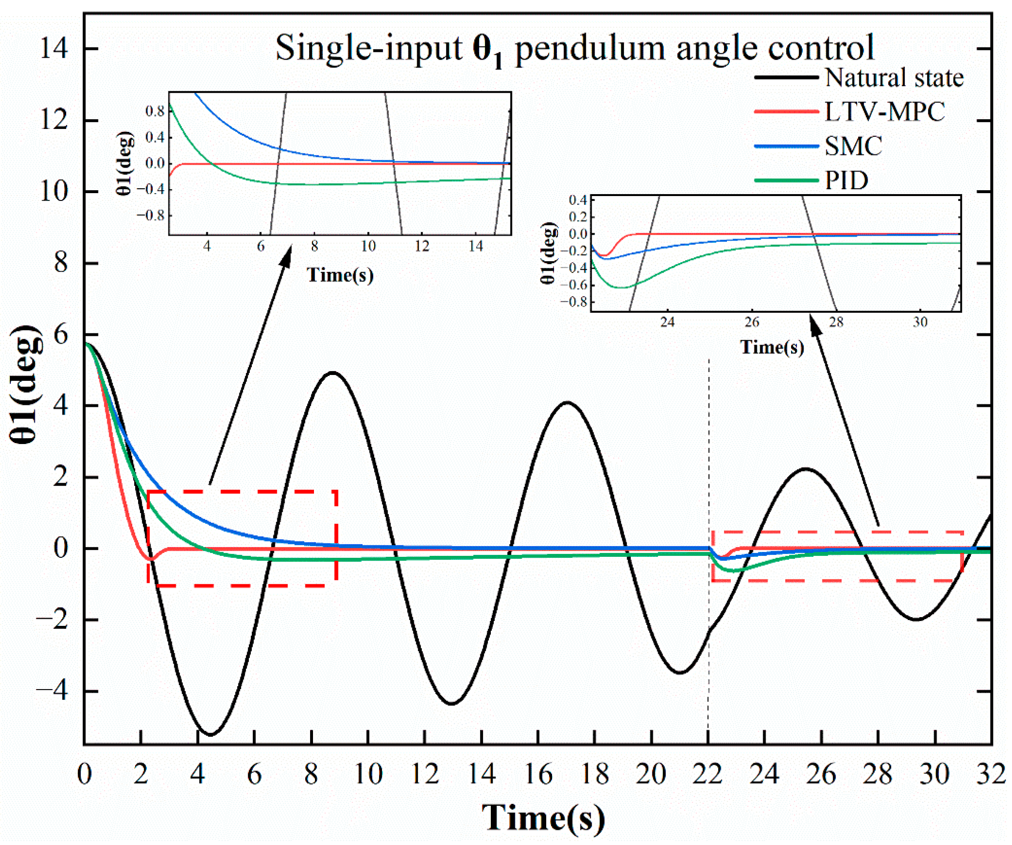
Focusing on single-input control using the luffing angle, α, a comparative analysis assessed the effectiveness of LTV-MPC in suppressing payload oscillations during crane luffing and slewing operations. The performance of LTV-MPC was compared with the uncontrolled system response, SMC, and PID control. Single-input ${\theta }_1$ pendulum angle control is shown in Figure 3.

Figure 3 illustrates the performance of single-input luffing control. Under LTV-MPC, the settling time for payload swing suppression was 3.05 s during luffing, with the control input active between 0.75 s and 3.25 s. The system settled within 0.007° of the equilibrium point (set to 0°). During slewing, swing suppression in the luffing direction was achieved in 1.15 s (starting at 22 s), with control input applied from 21.95 s to 23.4 s and settling within 0.003° of equilibrium.

In contrast, SMC required 7.5 s to suppress swing during luffing (control input: 0.25 s to 7.4 s), settling within 0.154° of equilibrium. During slewing, suppression in the luffing direction took 3.5 s (total time: 25.5 s; control input: 22.65 s to 28.1 s), achieving a residual deviation of 0.069°.

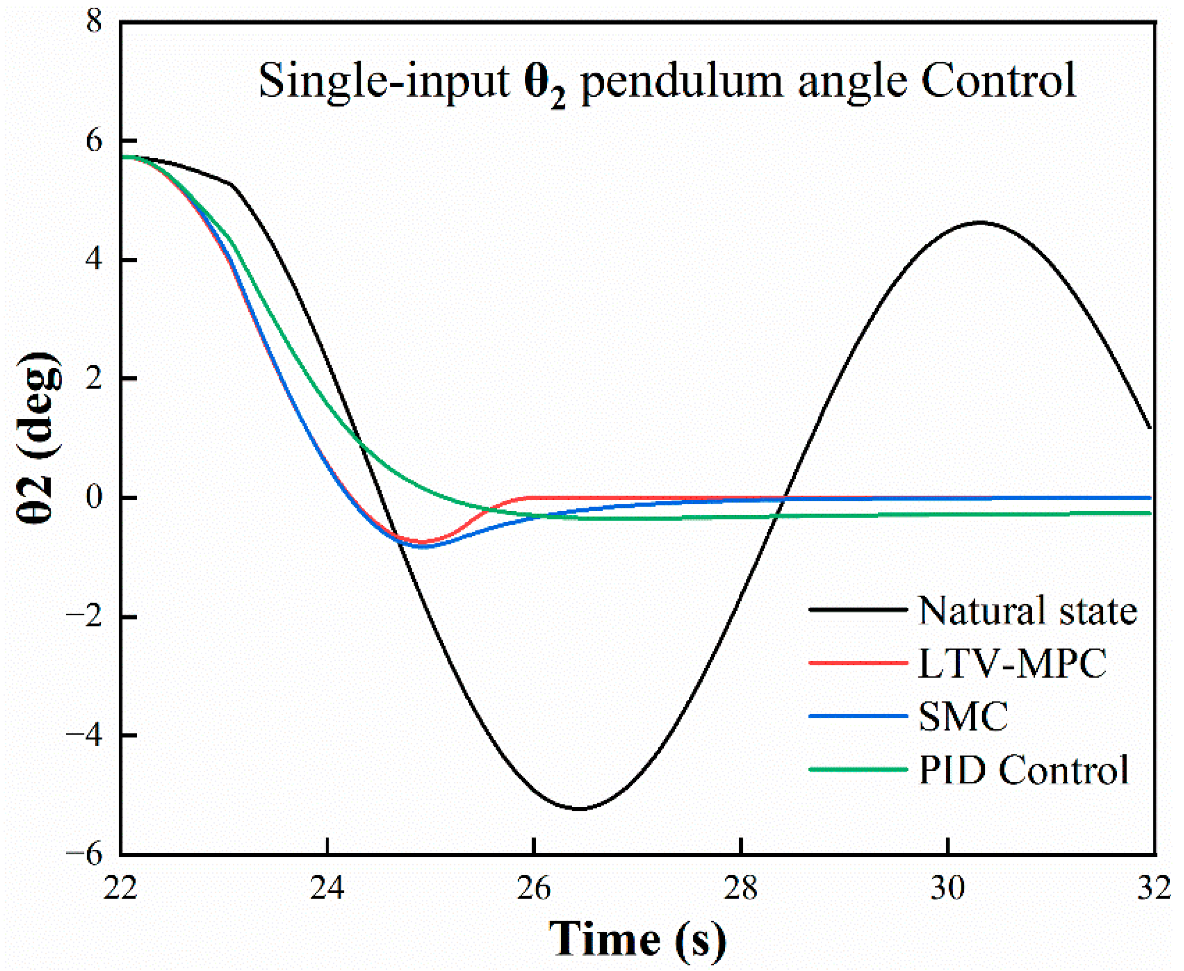
Similarly, PID control required 8 s for swing suppression during luffing (control input: 0.15 s to 6.5 s), settling within 0.321° of equilibrium. During slewing, suppression required 4.35 s (total time: 26.35 s; control input: 22.2 s to 27.6 s), resulting in a residual deviation of 0.136°. Single-input ${\theta }_2$ pendulum angle control is shown in Figure 3.

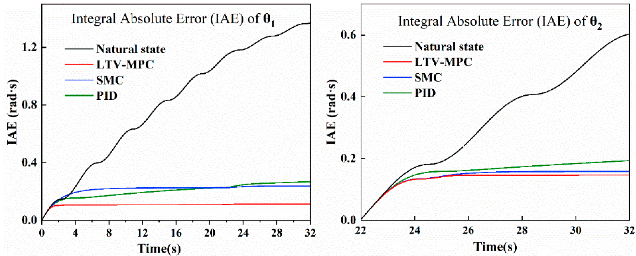
Figure 4 demonstrates the performance of single-input slewing control. Under LTV-MPC, swing during slewing was suppressed within 4.45 s (total time: 26.45 s), with control input applied from 22.95 s to 26.7 s. The system settled within 0.015° of the equilibrium point and maintained stable swing angles throughout the remaining simulation duration. In comparison, SMC required 5.15 s (total time: 27.15 s) to suppress swing during slewing (control input: 22 s to 22.65 s), settling within 0.04° of equilibrium. PID control achieved swing suppression in 4.05 s (total time: 26.05 s) during slewing (control input: 22 s to 26.6 s), resulting in a residual deviation of 0.28° from equilibrium. Comparison of IAE curve performance is shown in Figure 5.

In the integral absolute error (IAE) curve, a smaller value indicates superior performance, while a larger value corresponds to greater deviations. Figure 5 compares the error accumulation of θ₁ and θ₂ under four scenarios: the uncontrolled state and three control strategies—LTV-MPC, SMC, and PID. The corresponding IAE data are presented in

Table 5. IAE data indicators.

Status and Strategy	${\mathit{\theta }}_1$	${\mathit{\theta }}_2$
Natural state	1.37	0.6
LTV-MPC	0.11	0.15
SMC	0.24	0.16
PID	0.27	0.19

.

As shown in Table 5, under the natural state, the IAE of ${\theta }_1$ reaches 1.37, and that of ${\theta }_2$ reaches 0.6. Figure 5 indicates that the error accumulates rapidly over time in this case, demonstrating a large system error and poor stability without control. In contrast, the LTV-MPC strategy achieves an IAE of 0.11 for ${\theta }_1$ and 0.15 for ${\theta }_2$, which are the lowest among the three control methods. The corresponding curves show that error accumulation increases very slowly and stabilizes rapidly, indicating the best control performance. The SMC method results in an IAE of 0.24 for ${\theta }_1$ and 0.16 for ${\theta }_2$, outperforming PID but slightly inferior to LTV-MPC, thus ranking second in control effectiveness. The PID controller yields the highest IAE values among the three strategies, with 0.27 for ${\theta }_1$ and 0.19 for ${\theta }_2$, accompanied by greater error accumulation and less effective control performance.

Based on the IAE metric, it can be concluded that the LTV-MPC control demonstrates the best performance in suppressing error accumulation for both ${\theta }_1$ and ${\theta }_2$, followed by SMC, while PID exhibits relatively weak effectiveness. In contrast, the natural state leads to severe error accumulation, indicating that the introduction of control strategies significantly enhances both the precision and stability of the system.

Based on the single-input control curves and IAE results presented above, the following conclusions are drawn regarding payload swing suppression: During luffing, both SMC and PID control require longer settling times and exhibit larger steady-state deviations from equilibrium compared to LTV-MPC. Continuous minor control inputs are also required to maintain stability after initial suppression. In contrast, LTV-MPC achieves superior stability under equivalent conditions. During slewing, while PID control initially approaches equilibrium most rapidly, it requires extended stabilization time and results in larger residual deviations, resulting in higher energy consumption for stability maintenance. Conversely, LTV-MPC converges most rapidly to equilibrium and attains the closest proximity to it. From a practical engineering perspective—where safety and stability are paramount requirements—the experimental results confirm that LTV-MPC delivers the highest stability performance.

5.3. Comparison of Dual-Input Control Effects

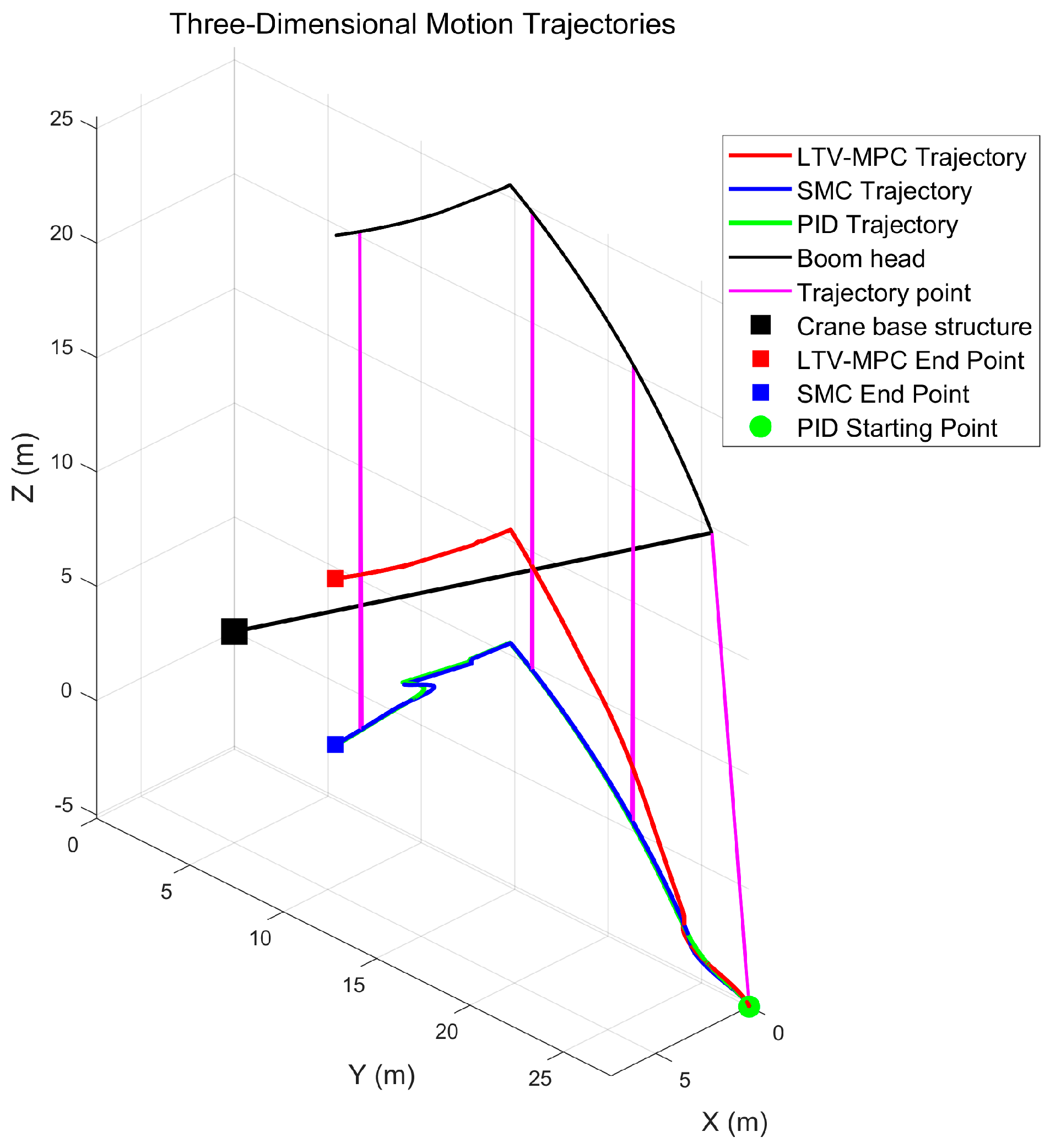
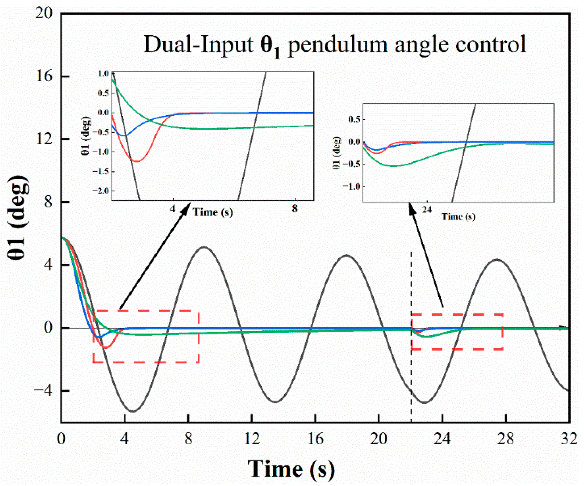
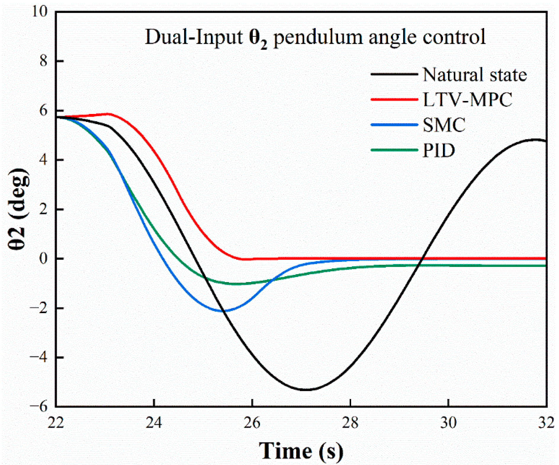
In the dual-input control scheme, the luffing angular rate and rope hoisting rate are designated as the two control inputs. Through coordinated variation in these inputs, the system enables effective payload swing suppression while ensuring operational stability. The comparative trajectory tracking performance of the three control strategies is illustrated in Figure 6.

Figure 6 presents payload trajectory tracking curves for the three-dimensional crane system, implemented on the Matlab/Simulink (R2022b) simulation platform. The figure compares trajectories under four scenarios: the uncontrolled state and three control strategies—LTV-MPC, SMC, and PID. Dual-input amplitude swing angle control efficacy is shown in Figure 7.

Figure 7 illustrates the swing angle control performance under a dual-input configuration. With LTV-MPC control, the settling time for swing suppression during the luffing process is 4.3 s, with a residual deviation of 0.009° from the equilibrium point. During slewing operations, swing suppression in the luffing direction is achieved within 1.45 s (23.45 s total), settling merely 0.0008° from equilibrium and maintaining this precision until the simulation concludes. In contrast, the dual-input SMC method requires 4.85 s for luffing swing suppression, with control input active from 0.35 s to 4.5 s, resulting in a steady-state error of 0.015°. During slewing, it achieves suppression in 2.4 s (24.4 s total) through control input applied between 20.05 s and 25.5 s, settling within 0.011° of the equilibrium point. Similarly, PID control demonstrates a luffing settling time of 4.4 s with control input from 0.15 s to 6.5 s, yet it exhibits a significantly larger deviation of 0.4° after stabilization. During slewing operations, it requires 4.2 s (26.2 s total) for suppression, with control input spanning 22.2 s to 27.6 s, ultimately settling 0.047° from the target position. Dual-input rotary pendulum angle control efficacy is shown in Figure 8.

Figure 8 demonstrates the slewing swing angle control performance. The LTV-MPC method suppresses the slewing swing within 4.05 s (26.05 s total), achieving a minimal residual deviation of only 0.008° from the equilibrium point while exhibiting excellent robustness after suppression. In comparison, the SMC method requires 6.4 s (28.4 s total) to suppress the payload swing, with control input applied from 22 s to 28.2 s, resulting in a steady-state error of 0.028°. The PID control method takes 6.8 s (28.8 s total) to achieve suppression during the slewing process, with control input active between 21.95 s and 28.2 s, yet it leaves a considerably larger deviation of 0.288° from the equilibrium point. The results of the robustness test are shown in Figure 9, below.

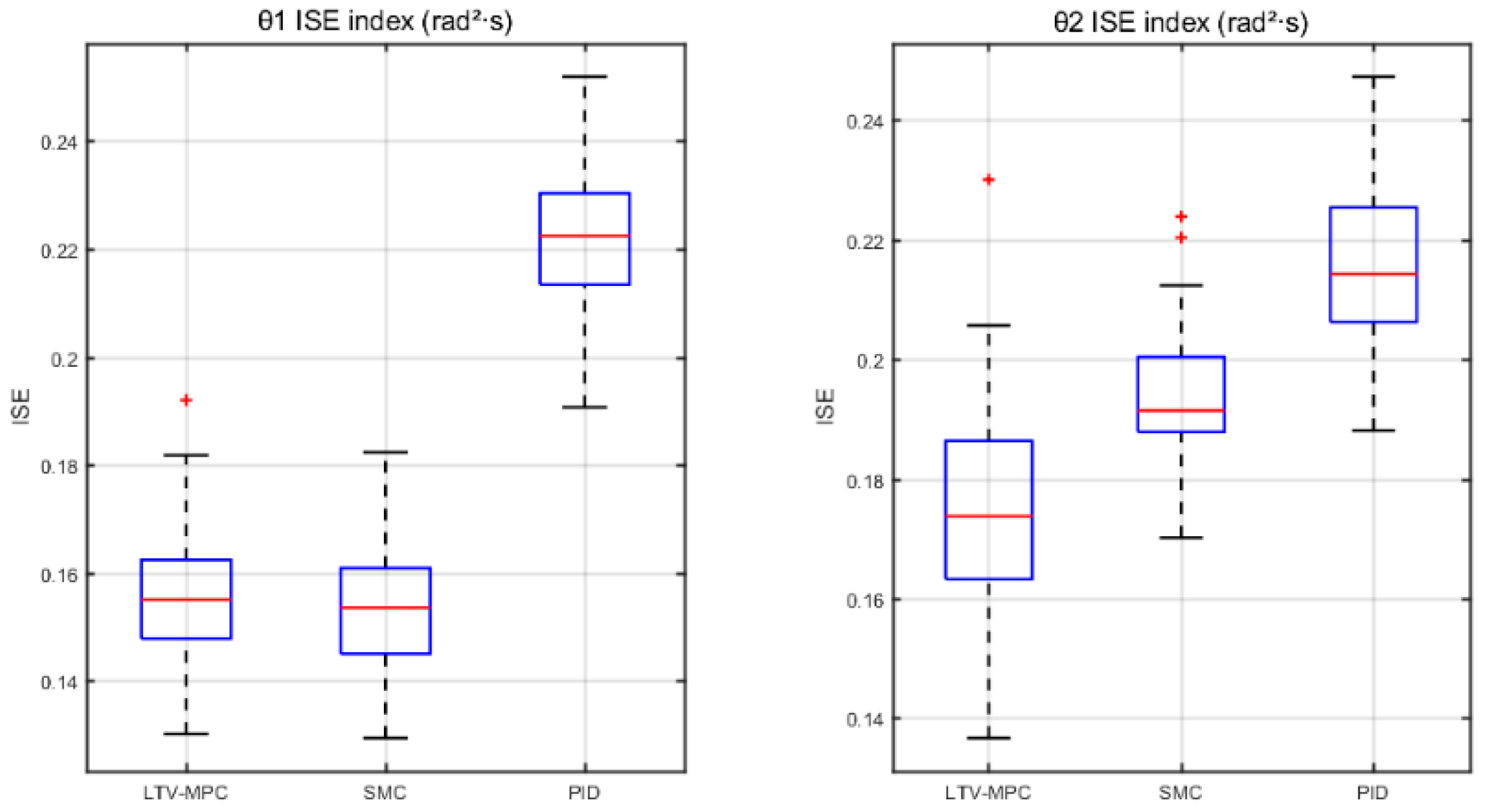
The robustness test results reflect the cumulative error of the sway angle over the entire operational time horizon, making it a more sensitive performance metric than the maximum sway angle. Red “+” indicates an outlier—an extreme value exceeding the whisker range—representing data deviating from the overall distribution. The “++” symbol denotes multiple outliers. A smaller mean value indicates higher control accuracy, while a smaller standard deviation signifies stronger robustness. The analysis is conducted separately for the ${\theta }_1$ direction (dominated by the lifting phase) and the ${\theta }_2$ direction (dominated by the slewing phase). The results are presented in

Table 6. ISE analysis in the ${\theta }_1$ direction.

Controller	Mean Value	Standard Deviation	Accuracy Ranking	Robustness Ranking
SMC	0.1545	0.0122	1	1
LTV-MPC	0.1562	0.0126	2	2
PID	0.2222	0.0133	3	3

and

Table 7. ISE analysis in the ${\theta }_2$ direction.

Controller	Mean Value	Standard Deviation	Accuracy Ranking	Robustness Ranking
LTV-MPC	0.1753	0.0174	1	1
SMC	0.1943	0.0113	2	2
PID	0.2159	0.0140	3	3

.

The underlying mechanisms are analyzed based on the data presented in Table 6, above. The invariance principle of sliding mode control renders it insensitive to parameter variations in mass and damping. The designed boundary layer ($\varphi$ = 0.05) suppresses chattering while preserving a fast disturbance rejection capability, resulting in minimal cumulative error with low oscillation. The predictive mechanism of LTV-MPC (with $N_p$ = 30) enables anticipatory compensation for changes in the elevation angle. However, time-varying parameters lead to a model–plant mismatch, necessitating online matrix updates that introduce minor errors. Consequently, it exhibits a marginally higher mean value and slightly greater fluctuations compared to SMC.

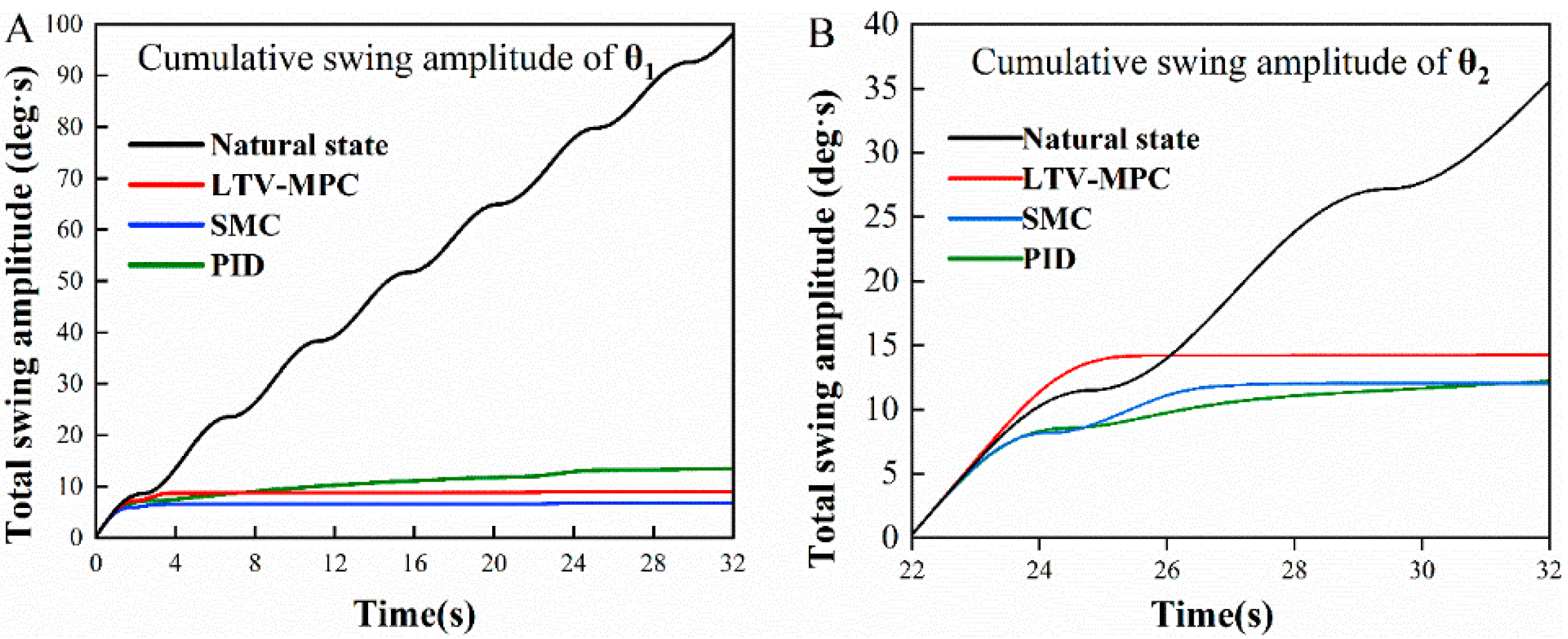
The underlying mechanisms are analyzed based on the data presented in Table 7. During the slewing phase, LTV-MPC activates the $dd\beta$ control channel, where its prediction horizon enables advance planning of control inputs to compensate for dynamic disturbances induced by slewing angular acceleration. The time-varying model adapts to phase nonlinearities, resulting in minimal ISE. By contrast, the sliding surface, $s_2={\lambda }_2{\theta }_2+{\dot{\theta }}_2$, in SMC exhibits slight dynamic tracking lag relative to LTV-MPC’s predictive mechanism. During the slewing acceleration phase, the switching gain, $k_2$ = 1.0, provides insufficient speed for disturbance rejection. However, the inherent robustness of sliding mode control results in the smallest standard deviation and the most stable oscillations. The cumulative angular displacement curve is shown in Figure 10.

Figure 10 presents the cumulative swing amplitude curves and ISE metric, comparing the θ₁ and θ₂ swing accumulation characteristics across the uncontrolled state and three control strategies (LTV-MPC, SMC, PID). The cumulative amplitude curve reflects angular deviation progression over time, where lower values indicate enhanced swing suppression. Similarly, reduced ISE values denote diminished squared error accumulation, signifying superior control precision.

In Figure 10A, From an overall trend perspective, in the cumulative swing amplitude of θ₁, the curve under the natural state rises rapidly, approaching approximately 100°·s around 30 s, indicating severe swing accumulation. In contrast, under the control of LTV-MPC, SMC, and PID, the curves remain almost flat, maintaining an extremely low accumulation level, demonstrating that the control strategies effectively suppress the swing accumulation of θ₁. In Figure 10B, Regarding the cumulative swing amplitude of θ₂, the curve under the natural state also surges rapidly, exceeding 35°·s around 30 s. Under the control strategies, the curve’s increase is significantly lower than that in the natural state. The cumulative swing amplitudes for LTV-MPC, SMC, and PID are maintained at approximately 15°·s, 12°·s, and 12°·s, respectively, indicating substantial suppression of swing. The quantitative ISE comparison across strategies is detailed in

Table 8. ISE data indicators.

Control Strategy	${\mathit{\theta }}_1$	${\mathit{\theta }}_2$
LTV-MPC	34.72	71.12
SMC	34.72	43.97
PID	31.29	40.61

.

As indicated in Table 6, SMC achieves optimal θ₁ ISE performance, whereas PID yields superior θ₂ ISE results. This outcome stems from LTV-MPC’s “model prediction and rolling optimization” logic: for time-varying systems, it tolerates certain transient error fluctuations to ensure stability and tracking rapidity. Although these fluctuations exhibit minimal absolute error accumulation (reflected in superior IAE performance), their instantaneous squared values are amplified by the ISE metric, resulting in comparatively higher ISE values.

Based on the dual-input control curve results, all three methods demonstrate comparable initial payload suppression times at luffing motion onset. However, LTV-MPC maintains the closest proximity to the equilibrium point, whereas PID exhibits the largest deviation. During slewing operations, specifically in luffing-direction control, both LTV-MPC and SMC deliver satisfactory performance.

Comparative analysis of single-input and dual-input scenarios reveals that while PID achieves payload swing suppression, it incurs larger equilibrium deviations and higher energy consumption. Although SMC approaches LTV-MPC’s suppression performance, its efficacy depends critically on sliding surface design and suffers from inherent chattering. This suppression comes at the cost of stability compromise, limiting practical viability in engineering applications. Conversely, LTV-MPC ensures smooth process transitions, effective swing suppression, minimal equilibrium deviation, reduced energy consumption, and enhanced stability. The proposed LTV-MPC method necessitates solving high-dimensional QP problems iteratively. Computational overhead escalates significantly during rapid parameter fluctuations, potentially inducing control latency. Furthermore, multivariate coupling in the crane sway system increases QP dimensionality. Additionally, current disturbance modeling incorporates only structured perturbations, excluding unstructured disturbances like platform vibration. In practical applications, external disturbances typically exhibit persistent and time-varying characteristics.

In 2024, Zhao [25] et al. from Wuhan University of Science and Technology designed control methods for a tower crane under different sway conditions to achieve precise positioning and sway suppression. By adjusting the damping coefficient, anti-sway control was implemented during variations in trolley displacement and slewing angle. Their best-reported results achieved a settling time of approximately 7 s with a residual sway angle within 2°. In contrast, our method completely suppresses oscillation during luffing and slewing operations within 5 s while maintaining the residual sway angle below 0.5°, demonstrating superior performance.

6. Suspended Load Experimental Platform

Due to practical constraints in full-scale experimentation, a scaled crane prototype was assembled at the Shanxi Key Laboratory of Intelligent Logistics Equipment. The YOLO v12 algorithm was employed for suspended load detection.

6.1. Experimental Platform Construction

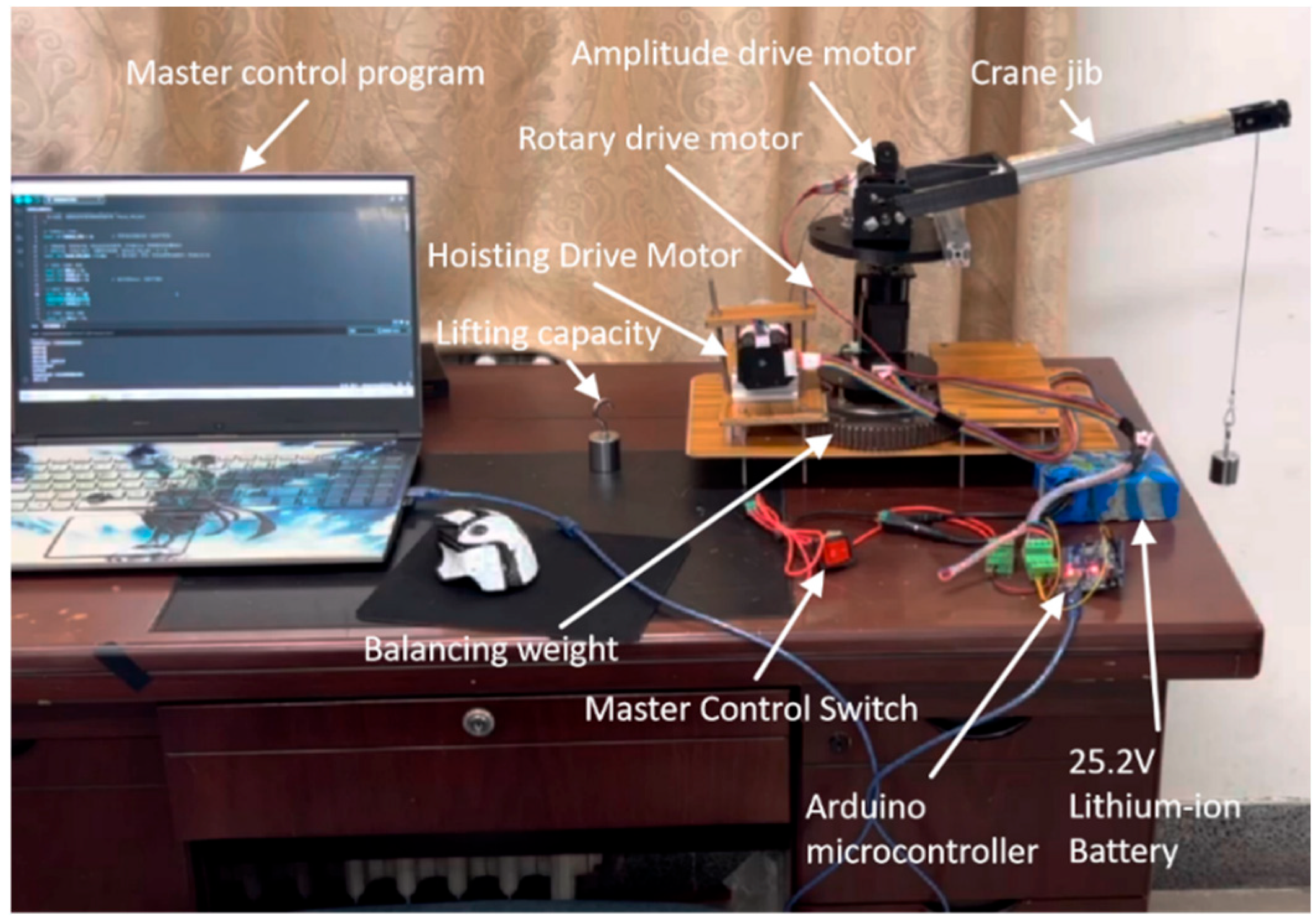
The experimental platform comprises three gear motors governing luffing, slewing, and wire rope actuation. Post-assembly and electrical integration, operational integrity was verified prior to experimentation. The configured platform structure is illustrated in Figure 11.

Figure 11 documents all experimental equipment captured within the Shanxi Provincial Key Laboratory of Intelligent Logistics Equipment. Corresponding to the platform configuration in Figure 11, technical specifications for critical components were compiled and are presented in

Table 9. Key equipment technical specifications.

Equipment Name	Model/Specification	Core Technical Parameters
Gear Motor (Yixing Technology, Wenzhou, China)	42HS4815A4	Reduction ratio: 5.2; Holding Torque: 3.6 kg · cm; Rated Output Torque: 0.55 N · m; Body Length: 48 mm; Step Angle: 1.8°;
Stepper Closed-Loop Driver (ZDT, Guangzhou, China)	42 Stepper closed-loop driver	Mainboard Model: Emm42_V5.0; Main Control Chip: Cortex-M4F Core; Control Mode: Pulse Control; Supply Voltage: 9–28 V DC; Rated Operating Current: 0–3000 mA (Continuous Output)
Boom(Bingcheng Metal Manufacturing Plant, Hangzhou, China)	European standard 2020L-1.5 aluminum profile	Usable Length: 40 cm; Cross-Sectional Dimensions: 20 mm × 20 mm; Linear Weight: 0.47 kg/m
Wire Rope (Hongyi Steel Rope, Guangzhou, China)	304 stainless steel core	Diameter: 1.5 mm (Suitable for a 500 g load)
Counterweight (Bora Machinery, Yantai, China)	Annular Counterweight	Dimensions: Outer Diameter 160 mm × Inner Diameter 80 mm × Height 27 mm; Mass: 5.5 kg; Material: HT200 Gray Cast Iron
Hoisted load (Hengshi Technology, Ningbo, China)	Standard Weight	Specification: 500 g; Accuracy Class: M1 Class; Surface Finish: Mirror Polish
Microcontroller (Chuanglebo, Changsha, China)	Arduino UNO R3	Core Control Chip: ATmega328P; Operating Voltage: 5 V; Programming Environment: VSCode (with PlatformIO plugin);

.

6.2. Experiment Result

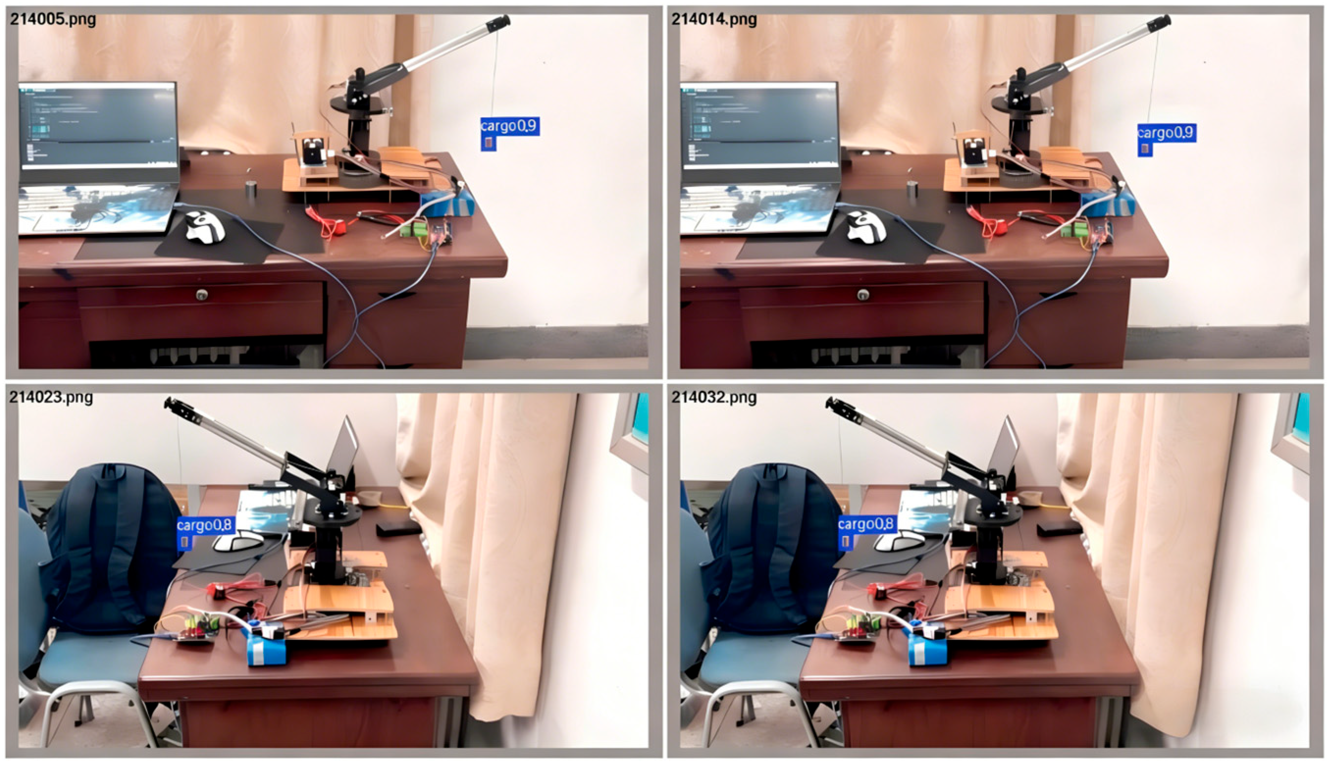
To comprehensively validate the LTV-MPC strategy’s efficacy in payload swing suppression during all-terrain crane lifting operations, a series of controlled hoisting tests was conducted on the experimental platform. For precise trajectory acquisition, the YOLOv12 deep learning architecture was meticulously trained and utilized, generating four comparative datasets under uncontrolled and LTV-MPC-controlled conditions during luffing and slewing maneuvers. Due to substantial image data volume, space limitations preclude full visualization; consequently, a selective approach presents only luffing-motion results herein. Corresponding batch annotation outputs detailing payload detection performance are detailed in Figure 12.

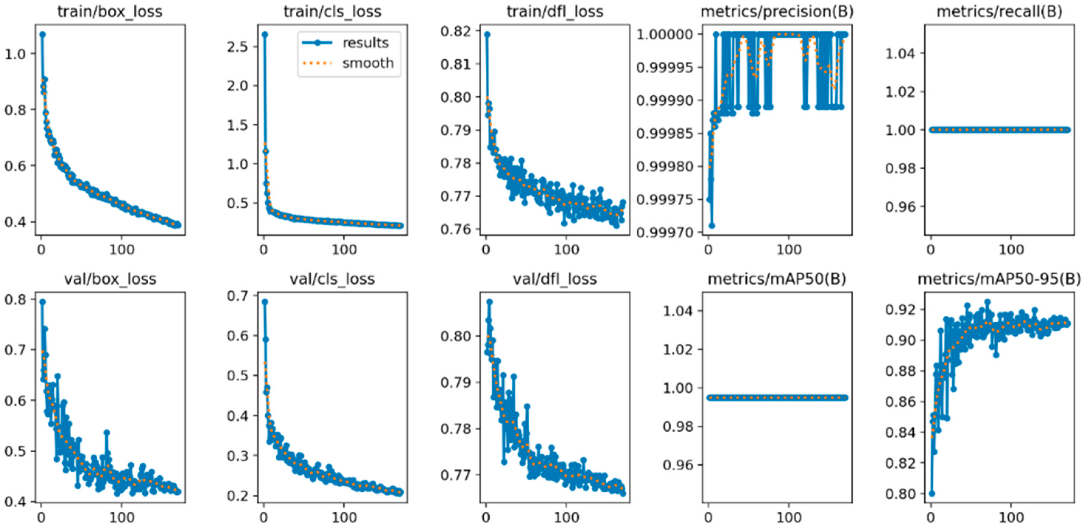
Figure 13 depicts critical loss metrics during model training. These curves collectively demonstrate stable convergence behavior throughout the training epochs. A total of 1750 annotated object instances were utilized for model development.

The first row displays three training loss curves (train/box_loss, train/cls_loss, and train/dfl_loss). Specifically, train/box_loss represents the bounding box regression loss, with the horizontal axis indicating training epochs and the vertical axis showing the loss values. train/cls_loss denotes the classification loss; its rapid decline to a low level with subsequent stabilization reflects continuously decreasing classification errors and improving classification accuracy for categories in the training set. train/dfl_loss represents the distribution focal loss, which refines bounding box coordinate regression by predicting coordinates through probability distributions rather than fixed values.

The second row shows three validation loss curves (val/box_loss, val/cls_loss, val/dfl_loss), which reflect the model’s generalization capability on unseen data. All validation loss curves follow trends highly consistent with their training counterparts, with final loss values closely matching those of the training set. This indicates no significant overfitting, confirming excellent generalization performance on new data.

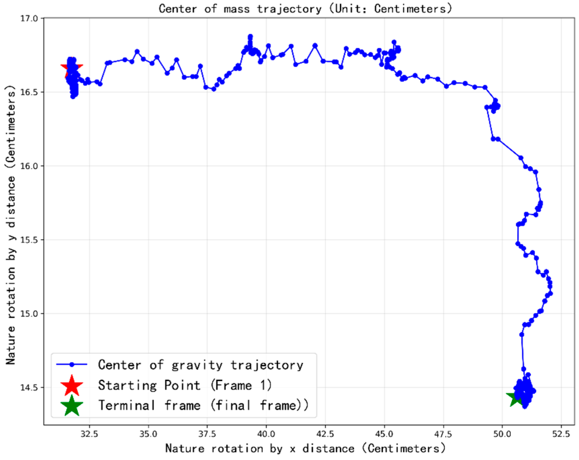
In the key metrics of the control algorithm under luffing conditions shown in Figure 13, the training set loss curves exhibit an overall declining trend with smooth progression, while the validation set loss curves also show a descending trend and appear significantly more stable compared to the natural state during luffing operations. This indicates that the gear motor, combined with the LTV-MPC method, can effectively maintain stability while successfully reducing payload swing. Among the remaining four subplots, metrics/precision (B) approaches 1.0, metrics/recall (B) remains stable around 1.0, metrics/mAP50 (B) (mean average precision at IoU ≥ 0.5) converges close to 1.0, and metrics/mAP50-95 (B) (mean average precision over IoU 0.5–0.95) shows a continuous upward trend. These results demonstrate excellent convergence of the model training, with validation loss trends consistent with the training set and no significant overfitting. The strong generalization capability, along with core metrics such as precision, recall, and mAP, all approaching 1.0, sufficiently confirms the highly successful training of the object detection model. Trajectory tracking under natural state variation conditions is shown in Figure 14.

Figure 14 shows a chaotic, irregular trajectory under natural luffing. Dense point clusters with large, unpredictable fluctuations in the initial region indicate severe cargo oscillations and poor stability. The considerable start–end point separation and absence of clear direction reveal random, oscillatory motion with poor convergence and uncontrolled movement. This erratic pattern causes significant payload swinging, reducing precision and risking crane instability, thereby compromising safety and efficiency trajectory tracking under variable amplitude control state conditions, as shown in Figure 15.

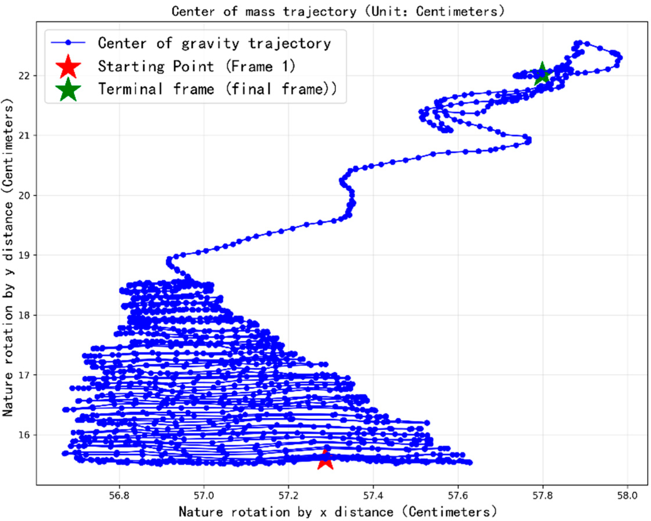
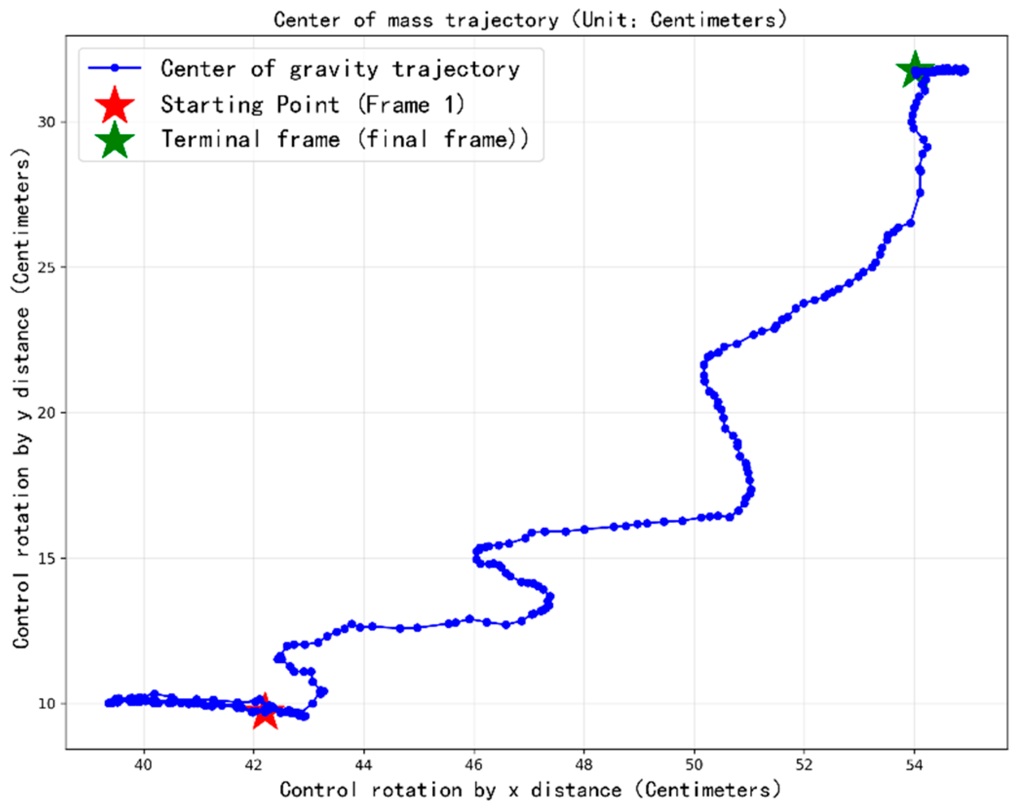
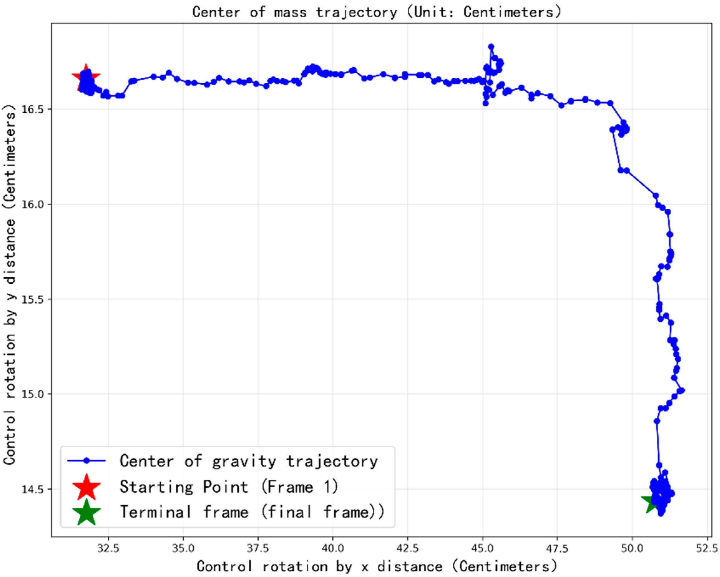
As shown in Figure 15, the luffing operation under the control algorithm produces a smooth and coherent trajectory, following a regular path from start to end without erratic fluctuations. The cargo’s center of gravity shows minimal oscillation, indicating substantially improved stability. Its movement progresses gradually and stepwise along the planned path toward the target, reflecting clear control objectives and favorable convergence. This demonstrates the ability of LTV-MPC to accurately plan the center of gravity trajectory. The resulting smooth and stable motion effectively reduces cargo swing, improves lifting precision, and enhances both safety and operational efficiency—particularly evident in high-precision, complex lifts where hoisting performance is significantly improved. Trajectory tracking under natural state reversion conditions is shown in Figure 16.

In Figure 16, within the intermediate region (x ≈ 37.5–45.0 cm, y ≈ 16.5–16.8 cm), the trajectory exhibits pronounced vertical oscillations with high frequency and large amplitude, indicating significant swinging of the cargo’s center of gravity in inertial space during natural slewing and poor stability. The trajectory lacks clear, stable directional guidance, and the fluctuations in the intermediate region represent irregular, ineffective oscillations. The path from the start to the end point shows poor controllability and convergence, reflecting the uncontrollable motion of the cargo’s center of gravity during natural slewing.

In Figure 17, the trajectory within the corresponding region (x ≈ 37.5–45.0 cm, y ≈ 16.5–16.8 cm) appears significantly smoother with pronounced suppression of oscillations, retaining only minimal local adjustments. The cargo’s center of gravity moves more steadily, demonstrating substantially enhanced stability. The path from start to end remains regular and continuous, exhibiting no excessive oscillations even in directional transition areas. The cargo’s center of gravity follows the planned trajectory with precision, showing strong convergence and well-defined control objectives, which reflects LTV-MPC’s accurate regulation capability for slewing trajectories.

The experimental platform employs a geometrically scaled model (scale factor κ = 1:75) featuring a 0.4 m maximum boom length and 0.5 kg payload capacity, while simulation parameters replicate a full-scale crane (29.5 m boom, 1000 kg payload). Although dynamic similarity was maintained for fundamental sway modes, significant scale effects remain unaddressed. Full-scale boom flexibility (EI ≈ 10⁹ N·m²) induces multimodal vibrations absent in the rigid aluminum profiles (EI ≈ 10⁴ N·m²) of the scaled model. Wire rope elasticity (E = 1.1 × 10¹¹ Pa) in industrial cranes causes 0.8–1.2% dynamic length variations, a phenomenon not captured by the scaled model’s stiffer steel cables (E = 2.1 × 10¹¹ Pa, diameter 1.5 mm). Environmental factors like wind resistance (Re > 10⁶) generate nonlinear disturbances negligible at the scaled model’s Reynolds number (Re ≈ 10⁴). Additionally, industrial hydraulic actuators achieve 0–300-bar pressure transitions in under 100 ms, outperforming the scaled gear motors’ bandwidth.

These limitations stem from laboratory constraints, including spatial restrictions (<100 m²), safety protocols, and budgetary caps (<USD 15 k), precluding full-scale validation.

7. Conclusions

Based on the Matlab/Simulink simulation results, comparison between single- and dual-input control reveals that in single-input control, the LTV-MPC method demonstrates optimal performance in both luffing and slewing processes regarding both settling time and post-suppression stability. In luffing control, the mean value is slightly lower than SMC. This is due to time-varying parameters leading to a model–plant mismatch, necessitating online matrix updates that introduce minor errors. Consequently, it exhibits a marginally lower mean value. In slewing control, although LTV-MPC achieves the lowest mean value, its standard deviation remains low. While LTV-MPC demonstrates superior overall robustness, it also faces challenges in compensating for dynamic disturbance delays.

In the experimental platform tests, comparison between the natural state and LTV-MPC control under both luffing and slewing conditions shows that LTV-MPC contributes to noticeable swing suppression according to the experimental data. Therefore, for both single- and dual-input control scenarios, LTV-MPC exhibits superior performance compared to SMC and PID strategies in maintaining stability while suppressing payload swing in all-terrain crane operations.

For future research, efforts can be directed along the following three avenues. First, we can design an adaptive horizon strategy that dynamically adjusts $N_p$ and $N_c$ based on the magnitude of the sway angle error (reducing the horizon when the error is small to decrease computational load). Second, we can introduce stochastic process models (e.g., Gaussian white noise; Markov processes) to simulate dynamic wind resistance and platform vibrations, thereby refining disturbance scenario design. A “rigid + flexible” coupled multibody dynamics model should be established to comprehensively account for the flexible characteristics of the boom and wire ropes. This involves incorporating flexible factors into the simulation model, such as an Euler–Bernoulli beam model for the boom and a spring-damper model for the wire rope to enhance consistency between simulation and reality. Third, we can construct a medium-scale experimental testbed equipped with industrial-grade actuators and sensors to mitigate scale effects. Hardware-in-the-loop (HIL) simulation experiments can then be conducted by coupling the actual controller with a high-fidelity simulation model, striking a balance between experimental authenticity and cost control.

References

1. Liang, C. Research on Coupling Suppression Control and Experiment of Crane Operation and Load Swing; Southwest Jiaotong University: Chengdu, China, 2019; p. 000418. [Google Scholar]
2. Chen, H.; Yang, T.; Sun, N.; Fang, Y. Motion Trajectory-Based Transportation Control for 3-D Boom Cranes: Analysis, Design, and Experiments. IEEE Trans. Ind. Electron. 2019, 66, 3636–3646. [Google Scholar] [CrossRef]
3. Tayfun, A.; Soyguder, S. Real-time control and application with self-tuning PID-type fuzzy adaptive controller of an inverted pendulum. Ind. Robot 2019, 46, 159–170. [Google Scholar]
4. Lee, D.; Kim, T.-W.; Ji, S.-W.; Kim, Y.-B. A study on load position control and vibration attenuation in crane operation using sub-actuator. Meas. Control 2019, 52, 794–803. [Google Scholar] [CrossRef]
5. Charles, A.; Daniel, L.; Daniel, P.; Goran, A.; Igor, Š. Nonlinear modeling and robust LMI fuzzy control of overhead crane systems. J. Frankl. Inst. 2020, 358, 1376–1402. [Google Scholar]
6. Bernardo, C.; de Lima, L.E.M. Anti-balance Load Control System Applied to an Overhead Crane Prototype Activated by Voice Commands. IEEE Lat. Am. Trans. 2021, 19, 834–843. [Google Scholar] [CrossRef]
7. Johan, K.; Ebbesen, M.K.; Hansen, M.R. Anti-swing control of a hydraulic loader crane with a hanging load. Mechatronics 2021, 77, 102599. [Google Scholar] [CrossRef]
8. Hu, D.; Qian, Z.; Fang, Y.; Chen, Y. Modeling and nonlinear energy-based anti-swing control of underactuated dual ship-mounted crane systems. Nonlinear Dyn. 2021, 106, 1–16. [Google Scholar] [CrossRef]
9. Luo, K.; Teng, R.; Fan, C. Research on the Lifting and Luffing Coordination Strategy of All-Terrain Cranes. Chin. J. Constr. Mach. 2021, 19, 313–317. [Google Scholar]
10. Tian, G.; Huang, J.; Singhose, W. Eccentric-load dynamics and oscillation control of industrial cranes transporting heterogeneous loads. Mech. Mach. Theory 2022, 172, 104800. [Google Scholar] [CrossRef]
11. Shi, H.; Yao, F.; Yuan, Z.; Tong, S.; Tang, Y.; Han, G. Correction to: Research on nonlinear coupled tracking controller for double pendulum gantry cranes with load hoisting/lowering. Nonlinear Dyn. 2022, 109, 1253. [Google Scholar] [CrossRef]
12. Bilgin, B.; Melek, E. Heave and horizontal displacement and anti-sway control of payload during ship-to-ship load transfer with an offshore crane on very rough sea conditions. Ocean. Eng. 2023, 267, 113309. [Google Scholar]
13. Fan, B.; Zhang, Y.; Sun, L.; Wang, L.; Liao, Z. Passivity and underactuated modeling-based load energy coupling control for three-dimensional overhead crane systems. Mechatronics 2023, 96, 103062. [Google Scholar] [CrossRef]
14. Sun, M.; Luan, T.; Tan, Z.; Wang, W. Swing Reduction Control of Ship Crane Based on Rope Length Change. Arab. J. Sci. Eng. 2023, 48, 15597–15608. [Google Scholar] [CrossRef]
15. Yu, Z.; Dong, H.; Liu, C. Research on Swing Model and Fuzzy Anti Swing Control Technology of Bridge Crane. Machines 2023, 11, 579. [Google Scholar] [CrossRef]
16. Tong, S.; Shi, H.; Zhou, P.; Xu, W.; Ma, J. Research on accurate motion control of cable crane based on variable structure sliding mode. J. Braz. Soc. Mech. Sci. Eng. 2023, 45, 316. [Google Scholar] [CrossRef]
17. Zhang, D.; Zhao, B.; Zhu, K.; Jiang, H. Dynamic Analysis of Full-Circle Swinging Hoisting Operation of a Large Revolving Offshore Crane Vessel under Different Wave Directions. J. Mar. Sci. Eng. 2023, 11, 197. [Google Scholar] [CrossRef]
18. Li, D.; Xie, T.; Li, G.; Yao, J.; Hu, S. Adaptive coupling tracking control strategy for double-pendulum bridge crane with load hoisting/lowering. Nonlinear Dyn. 2024, 112, 8261–8280. [Google Scholar] [CrossRef]
19. Wang, H.; Yang, W.; Yang, X.; Wang, J.; Shi, C. Fuzzy disturbance observer-based fuzzy swing suppression control of a ‘mooring-heavy lift crane-cargo’ coupled system. Intell. Mar. Technol. Syst. 2024, 2, 21. [Google Scholar] [CrossRef]
20. Segura, V.R.; Miranda-Colorado, R.; Rodriguez-Arellano, J.A.; Aguilar, L.T. Observer-based proportional-retarded controller for payload swing attenuation of 2D-crane systems including load hoisting-lowering. ISA Trans. 2024, 155, 15511–15517. [Google Scholar]
21. Kusznir, T.; Smoczek, J. Nonlinear Model Predictive Control with Evolutionary Data-Driven Prediction Model and Particle Swarm Optimization Optimizer for an Overhead Crane. Appl. Sci. 2024, 14, 5112. [Google Scholar] [CrossRef]
22. Lin, J.; Fang, Y.; Lu, B.; Cao, H.; Hao, Y. Constrained model predictive control for 3-D offshore boom cranes. Control. Eng. Pract. 2024, 142, 105741. [Google Scholar] [CrossRef]
23. Abut, T. An Inverted Pendulum System Control with Fuzzy Linear Quadratic Regulator Method: Experimental Validation. Comput. Mater. Contin. 2025, 85, 4023–4042. [Google Scholar] [CrossRef]
24. Fang, C.; Ma, J.; Wang, C.; Zhang, X. A Motion Planning-based Adaptive Control Method for an Underactuated Crane System. IEEE Trans. Control. Syst. Technol. 2012, 20, 241–248. [Google Scholar] [CrossRef]
25. Zhao, J. Research on the Positioning and Anti-Swing Method of Tower Crane Based on Sliding Mode Control; Wuhan University of Science and Technology: Wuhan, China, 2025. [Google Scholar]
Figure 1. All-terrain crane lifting system.
Machines 14 00024 g001
Figure 2. Three-dimensional coordinate system of an all-terrain crane.
Machines 14 00024 g002
Figure 3. Single-input amplitude control efficacy.
Machines 14 00024 g003
Figure 4. Single-input rotary control efficacy.
Machines 14 00024 g004
Figure 5. Comparison of IAE curve performance.
Machines 14 00024 g005
Figure 6. Trajectory tracking curves of the three control methodologies.
Machines 14 00024 g006
Figure 7. Dual-input amplitude swing angle control efficacy.
Machines 14 00024 g007
Figure 8. Dual-input rotary pendulum angle control efficacy.
Machines 14 00024 g008
Figure 9. Robustness test results.
Machines 14 00024 g009
Figure 10. Cumulative angular displacement curve.
Machines 14 00024 g010
Figure 11. Experimental platform demonstration.
Machines 14 00024 g011
Figure 12. Batch annotation results for object detection.
Machines 14 00024 g012
Figure 13. Visualization summary of key performance indicators for LTV-MPC control under variable amplitude operating conditions.
Machines 14 00024 g013
Figure 14. Trajectory tracking under natural state variation conditions.
Machines 14 00024 g014
Figure 15. Trajectory tracking under variable amplitude control state conditions.
Machines 14 00024 g015
Figure 16. Trajectory tracking under natural state reversion conditions.
Machines 14 00024 g016
Figure 17. Trajectory tracking under state reversal control conditions.
Machines 14 00024 g017