Dynamic Siting and Coordinated Routing for UAV Inspection via Hierarchical Reinforcement Learning

Abstract

To enhance the efficiency and reduce the operational costs of large-scale Unmanned Aerial Vehicle (UAV) inspection missions limited by endurance, this paper addresses the coupled problem of dynamically positioning landing/takeoff sites and routing the UAVs. A novel Hierarchical Reinforcement Learning (H-DRL) framework is proposed, which decouples the problem into a high-level strategic deployment policy and a low-level tactical routing policy. The primary contribution of this work lies in two architectural innovations that enable globally coordinated, end-to-end optimization. First, a coordinated credit assignment mechanism is introduced, where the high-level policy communicates its strategic guidance to the low-level policy via a learned “intent vector,” facilitating intelligent collaboration. Second, an Energy-Aware Graph Attention Network (Ea-GAT) is designed for the low-level policy. By endogenously embedding an energy feasibility model into its attention mechanism, the Ea-GAT guarantees the generation of dynamically feasible flight paths. Comprehensive simulations and a physical experiment validate the proposed framework. The results demonstrate a significant improvement in mission efficiency, with the makespan reduced by up to 16.3%. This work highlights the substantial benefits of joint optimization for dynamic robotic applications.

1. Introduction

In recent years, Unmanned Aerial Vehicles (UAVs) have been established as indispensable tools for a multitude of large-scale civilian and industrial operations [1,2,3]. The increasing demand for automated infrastructure inspection, particularly in domains such as power line maintenance, oil and gas pipeline surveillance, and post-disaster assessment, has highlighted the significant potential of UAV technology [4,5]. The automation of such tasks holds substantial socio-economic importance, offering the potential to reduce operational costs, enhance the reliability of critical infrastructure, and mitigate risks to human personnel in hazardous environments [6]. However, the operational range and autonomy of these platforms are fundamentally constrained by their limited battery endurance, which has emerged as a critical bottleneck for extended, fully autonomous missions [7,8]. A prevailing strategy to mitigate this limitation is the deployment of a network of landing and takeoff sites. These sites, acting as hubs for battery swapping or recharging, can theoretically enable continuous, long-duration missions. The overall efficiency of such a system, nevertheless, is critically dependent on the strategic placement of these sites [9].

To address the optimization of UAV operations, a significant body of research has been produced. The existing solutions can be broadly classified into two main categories: decoupled two-stage methods [10] and monolithic optimization methods [11].

Decoupled two-stage methods represent a conventional and widely adopted approach. In this paradigm, the problem is decomposed into two sequential sub-problems: a facility location problem (siting) followed by a Vehicle Routing Problem (VRP) [12]. For the initial siting stage, various algorithms have been employed to determine the optimal placement of a fixed number of sites. Classical optimization techniques, such as K-Means clustering for identifying task-dense areas [13] and mixed-integer linear programming (MILP) for formal optimization [14], are commonly utilized. Once the sites are fixed, the subsequent routing stage is addressed. A plethora of algorithms have been applied to this VRP sub-problem. Classical graph-based algorithms, including Dijkstra’s algorithm and A* [15], perform well in static environments but exhibit limited adaptability to dynamic changes. To handle more complex VRPs, heuristic and meta-heuristic algorithms have been extensively investigated. These include evolutionary approaches like genetic algorithms (GAs) [16] and swarm intelligence techniques such as particle swarm optimization (PSO) [17] and ant colony optimization (ACO) [18]. The primary drawback of all decoupled methods, however, is their inherent suboptimality. Since the siting decision is made without full knowledge of the optimal routes it will enable, the final solution is seldom globally optimal [19].

In contrast, monolithic optimization methods attempt to solve the siting and routing problems jointly within a single, unified framework to pursue global optimality. Traditional monolithic approaches often formulate the problem as a large-scale MILP [20] or a complex constraint satisfaction problem [21]. Due to the NP-hard nature of this joint optimization problem [22], the computational complexity of these exact methods grows exponentially with the problem scale, rendering them intractable for the large-scale, dynamic scenarios frequently encountered in real-world inspection missions.

With the advent of artificial intelligence, Deep Reinforcement Learning (DRL) has emerged as a powerful monolithic paradigm for solving complex sequential decision-making problems under uncertainty [23,24]. DRL-based agents can learn sophisticated policies directly from interaction with dynamic environments [25], making them a promising candidate for the PDFDRP. While DRL has been successfully applied to various UAV control problems, such as autonomous navigation [26,27] and data collection [28], applying a standard, “flat” DRL model to the joint siting and routing problem presents significant, unique challenges. The action space is vast and hybrid, and the sparse and significantly delayed rewards associated with a strategic siting decision make the credit assignment problem exceptionally acute [29]. This suggests that a more structured approach is necessary. While general-purpose Hierarchical Reinforcement Learning frameworks like Feudal Networks (FuN) [30] or the options framework [31] provide foundational ideas for temporal and state abstraction, they do not explicitly address the challenge of coordinating between distinct strategic (siting) and tactical (routing) domains, nor do they offer a natural mechanism for communicating fine-grained strategic preferences. A specialized hierarchical architecture is therefore required [32].

This leads to the central research questions of this paper: Can a hierarchical learning structure effectively decompose the complex joint problem while maintaining end-to-end optimization? And can specialized mechanisms be designed to facilitate efficient communication [33] and handle hard physical constraints within such a framework? To address these questions, this paper proposes a novel Hierarchical Reinforcement Learning (H-DRL) framework. The main innovations and contributions of this work are as follows:

• A Hierarchical Reinforcement Learning Framework for Joint Optimization. The dynamic UAV siting and routing problem is, for the first time, formulated and solved within an H-DRL framework. This architecture naturally decouples the problem into high-level strategic decisions and low-level tactical decisions, while a coordinated, end-to-end optimization process is maintained.
• A Coordinated Credit Assignment Mechanism via Intent Vectors. An innovative credit assignment mechanism is proposed. The high-level policy communicates its strategic “intent” to the low-level policy through a learned vector. This approach facilitates intelligent collaboration and addresses the credit assignment challenge inherent in hierarchical systems.
• An Energy-Aware Graph Attention Network (Ea-GAT) for Feasible Routing. A novel graph neural network, designated Ea-GAT, is designed for the low-level routing policy. By explicitly embedding an energy feasibility model into its attention mechanism, this network endogenously handles the UAV’s hard endurance constraints.

The remainder of this article is organized as follows. In Section 2, the problem formulation is presented. In Section 3, the proposed H-DRL framework is detailed. In Section 4, the feasibility and effectiveness of the proposed method are assessed. Finally, the conclusions are presented in Section 5.

2. Problem Formulation

This section provides a formal description of the dynamic UAV siting and routing problem. First, an overview of the system components and operational scenario is presented. Then, a mathematical model is established, defining the decision variables, objective function, and constraints. Finally, the problem is formulated as a Hierarchical Markov Decision Process (HMDP) to lay the groundwork for the proposed reinforcement learning solution.

2.1. System Overview

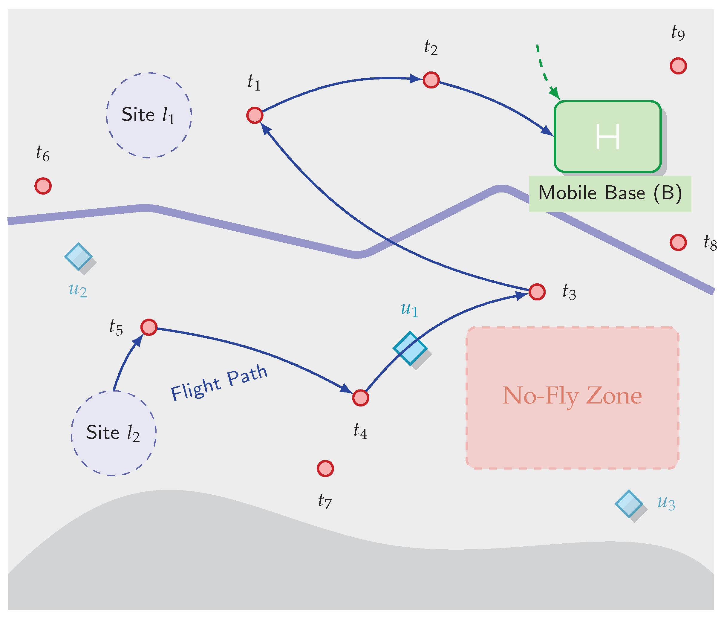
The operational scenario considered in this study involves a centralized system responsible for coordinating a fleet of UAVs to perform inspection tasks over a large geographical area. The key components of this system are illustrated in Figure 1.

The operational area is defined as a two-dimensional workspace $\mathcal{A}\subset {\mathbb{R}}^2$. Within this area, a set of inspection targets, denoted by $\mathcal{T}=\{t_1,t_2,\dots ,t_N\}$, must be visited by UAVs. Each target $t_i\in \mathcal{T}$ is characterized by its fixed coordinates ${\mathbf{p}}_i=(x_i,y_i)$ and a priority level, ${\rho }_i\in {\mathbb{R}}^{+}$. A higher value of ${\rho }_i$ indicates a more urgent or important task.

The system employs a fleet of M homogeneous UAVs, denoted by $\mathcal{U}=\{u_1,u_2,\dots ,u_M\}$. Each UAV is characterized by a maximum flight endurance $E_{max}$, which limits the maximum duration or distance of a single flight sortie, and is assumed to fly at a constant speed $v_{\mathrm{uav}}$.

Ground support is provided by a set of candidate locations for landing and takeoff sites, $\mathcal{L}=\{l_1,l_2,\dots ,l_K\}$, and a single mobile base, B. The base serves as the operational hub for UAVs to be launched, retrieved, and serviced (e.g., battery swapping), a process which takes a fixed time ${\tau }_b$. The mobile base can be repositioned to strategic locations and moves at a speed $v_{\mathrm{base}}$.

The dynamism of the problem is a key characteristic. The set of tasks is time-varying, denoted as $\mathcal{T}\left(k\right)$ at a discrete time step k. New tasks can be stochastically generated. Furthermore, the priorities of existing tasks can also change over time, i.e., ${\rho }_i\left(k\right)$. Similarly, environmental constraints, such as no-fly zones, can also be dynamic, denoted as $\mathrm{NFZ}\left(k\right)$ [34]. The proposed framework is designed to generate policies that are robust and adaptive to these real-time changes.

2.2. Mathematical Model

The problem is formally defined as the Dynamic UAV Facility Deployment and Routing Problem (PDFDRP). This problem is known to be NP-hard, as it combines complex aspects of both the facility location and vehicle routing problems [22]. The goal is to determine a joint policy for deploying the mobile base and routing the UAVs to minimize the overall mission completion time.

2.2.1. Decision Variables

The solution to the PDFDRP is a set of policies that determine two types of decisions over a time horizon. The first is the base deployment policy, which specifies the sequence of locations. ${\mathbf{p}}_B\left(k\right)$ for the mobile base B at different time steps k. The second is the UAV routing policy, which for each UAV $u_j$ and each sortie, defines an ordered sequence of tasks to visit, denoted by a path ${\mathcal{P}}_j=(t_{j1},t_{j2},\dots )$. The objective is to find the optimal set of policies that minimizes the overall makespan while satisfying all constraints.

2.2.2. Objective Function

The primary objective is to minimize the makespan, $J_{\mathrm{makespan}}$, which is defined as the time at which the last inspection task is completed. Let $C\left(t_i\right)$ be the completion time for task $t_i$. The objective function is given by

$$min{J}_{\mathrm{makespan}}=\underset{t_i\in \mathcal{T}}{max}\left\{C\left(t_i\right)\right\}$$

(1)

Minimizing the makespan implicitly encourages the system to reduce UAV flight time and base relocation time, thus capturing the trade-off between deployment and operational costs.

2.2.3. Constraints

A feasible solution to the PDFDRP must satisfy several operational constraints. First, the task coverage constraint requires that every task in the set $\mathcal{T}$ must be visited exactly once by a UAV.

The second and most critical constraint is the UAV endurance constraint. For any single flight sortie of a UAV, the total time consumed cannot exceed its maximum endurance $E_{max}$. A sortie consists of the flight from the base to a sequence of one or more tasks and the return flight to the base. Let a sortie’s path be a sequence of points $({\mathbf{p}}_{\mathrm{base}}^{\mathrm{start}},{\mathbf{p}}_1,\dots ,{\mathbf{p}}_k,{\mathbf{p}}_{\mathrm{base}}^{\mathrm{end}})$. The constraint is formulated as

$${\displaystyle \frac{\parallel {\mathbf{p}}_1-{\mathbf{p}}_{\mathrm{base}}^{\mathrm{start}}\parallel }{v_{\mathrm{uav}}}}+\sum _{i=1}^{k-1}{\displaystyle \frac{\parallel {\mathbf{p}}_{i+1}-{\mathbf{p}}_i\parallel }{v_{\mathrm{uav}}}}+{\displaystyle \frac{\parallel {\mathbf{p}}_{\mathrm{base}}^{\mathrm{end}}-{\mathbf{p}}_k\parallel }{v_{\mathrm{uav}}}}\le E_{max}$$

(2)

where $\parallel ·\parallel$ denotes the Euclidean distance.

Third, the path feasibility constraint dictates that the flight path of any UAV must not intersect with any no-fly zone.

Finally, the synchronization constraint ensures that a UAV must start and end its sortie at a designated base or site. Let $t_{\mathrm{start}}$ be the launch time and $t_{\mathrm{end}}$ be the retrieval time. The start and end waypoints of a sortie path must correspond to the facility location at the respective times.

The PDFDRP is an NP-hard problem, as it generalizes both the facility location and vehicle routing problems. The dynamic and coupled nature of the decisions motivates the use of a learning-based approach, which is detailed in the following sections.

2.3. Hierarchical Markov Decision Process Formulation

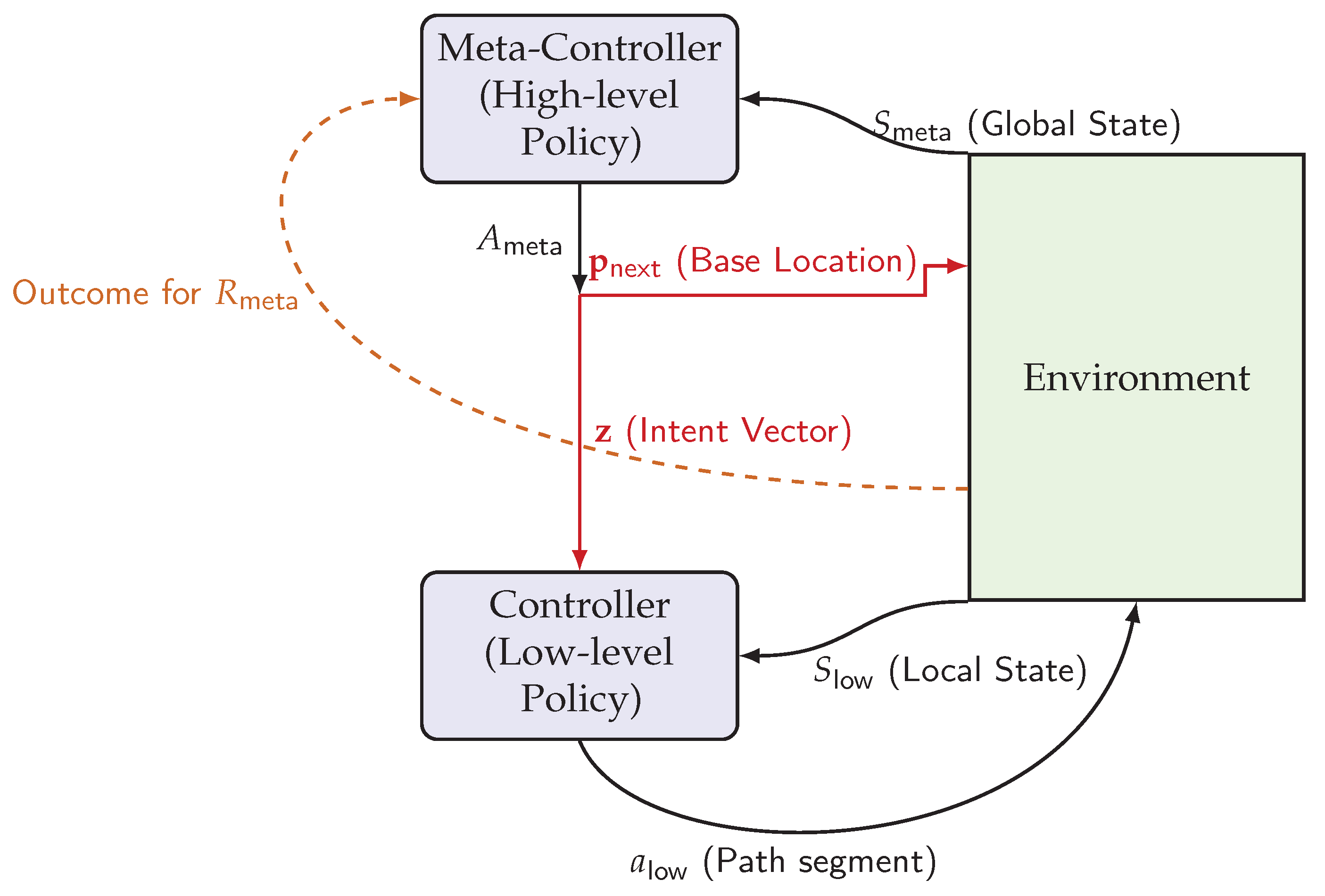
To effectively address the coupled and dynamic nature of the PDFDRP, the problem is formulated as a Hierarchical Markov Decision Process (HMDP) [30]. This hierarchical structure, illustrated in Figure 2, decomposes the complex, monolithic decision-making problem into two manageable, interconnected layers: a high-level (meta-controller) policy for strategic deployment and a low-level (controller) policy for tactical routing. The components of the high-level and low-level MDPs are defined below.

2.3.1. High-Level MDP

The high-level MDP is responsible for the strategic deployment of the mobile base B. Its objective is to learn a policy ${\pi }_{\mathrm{meta}}\left(A_{\mathrm{meta}}\right|S_{\mathrm{meta}})$ that maximizes the long-term cumulative reward.

The state $S_{\mathrm{meta}}\in {\mathbb{R}}^{H\times W\times C}$ provides a global, macroscopic snapshot of the entire mission, represented as a multi-channel feature map, suitable for processing by a convolutional neural network (CNN). It includes channels representing the spatial distribution of uncompleted tasks, the current locations of all UAVs, the location of the mobile base, and a map of known hazards.

The action $A_{\mathrm{meta}}=(l,\mathbf{z})$, where $l\in \{1,\dots ,K\}$ is the index of the selected candidate location and $\mathbf{z}\in {\Delta }^{K^{\prime }}$ is the intent vector, where ${\Delta }^{K^{\prime }}$ is the $(K^{\prime }-1)$-dimensional simplex. This composite action determines the next strategic location for the base and communicates tactical guidance to the low-level policy.

The reward $R_{\mathrm{meta}}$ is a delayed reward, calculated after the low-level policy has completed its sub-task. It is a function of the tasks completed, the cost of base relocation, and a term measuring consistency between the strategic intent $\mathbf{z}$ and the actual performance of the executed sorties.

2.3.2. Low-Level MDP

The low-level MDP is responsible for the tactical routing of a single UAV for one sortie. Its objective is to learn a policy ${\pi }_{\mathrm{low}}\left(A_{\mathrm{low}}\right|S_{\mathrm{low}})$ that generates an energy-feasible path to maximize the rewards defined by the intent vector.

The state $S_{\mathrm{low}}$ is formulated as a graph $\mathcal{G}=(\mathcal{V},\mathcal{E})$, where $\mathcal{V}$ is the set of nodes representing the UAV, assigned tasks, and base locations. This graph-based representation is highly effective for capturing the topological relationships in routing problems [35]. Each node $v\in \mathcal{V}$ is associated with a feature vector ${\mathbf{h}}_v\in {\mathbb{R}}^{D_v}$, including coordinates and remaining energy for the UAV node.

The action $A_{\mathrm{low}}\in {\mathcal{T}}_{\mathrm{unvisited}}$ is the selection of the next task to visit from the set of currently unvisited tasks for the current sortie.

The reward $R_{\mathrm{low}}$ is an immediate reward whose structure is dynamically modulated by the intent vector $\mathbf{z}$. It balances objectives such as path length, task completion, and safety, according to the high-level strategy. The detailed design of these components is presented in the next section.

3. The Proposed H-DRL Framework

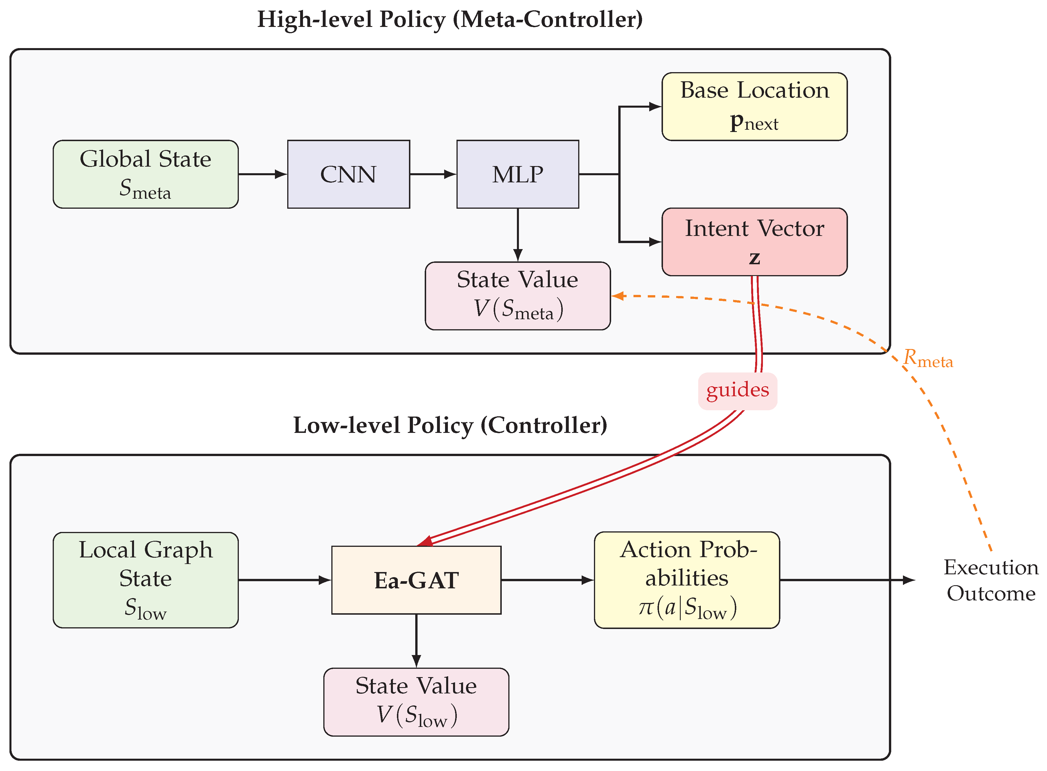
To solve the HMDP formulated in the previous section, a novel Hierarchical Reinforcement Learning (H-DRL) framework is proposed. This framework is designed to effectively manage the distinct responsibilities of strategic deployment and tactical routing through specialized high-level and low-level policies. The architecture enables end-to-end training, allowing the two policies to co-evolve and discover globally coordinated solutions. The overall architecture of the proposed framework is depicted in Figure 3, and the detailed design of each component is presented in the subsequent sections.

3.1. High-Level Policy for Proactive Deployment

The high-level policy, or meta-controller, is responsible for learning a long-term strategy for mobile base deployment. It operates at a lower frequency, making decisions at the beginning of each macro-episode, which typically encompasses one or more low-level sorties.

3.1.1. State Representation

The high-level state $S_{\mathrm{meta}}\in {\mathbb{R}}^{H\times W\times C}$ provides a global, macroscopic snapshot of the entire mission, formulated as a multi-channel image-like tensor. This representation is processed by a convolutional neural network (CNN) [36] to extract salient spatial features. The state consists of C channels, including the following: (1) a task density map, where each pixel value represents the number or cumulative priority of uncompleted tasks in that region; (2) a UAV location map, indicating the current positions of all UAVs; (3) a base location map, marking the position of the mobile base B; and (4) a hazard map, encoding the locations of static and dynamic no-fly zones.

3.1.2. Action Space

The meta-controller outputs a composite action $A_{\mathrm{meta}}=(l,\mathbf{z})$, where $l\in \{1,\dots ,K\}$ is the index of the selected candidate base location. The second component is the intent vector $\mathbf{z}\in {\mathbb{R}}^{K^{\prime }}$, which communicates strategic guidance to the low-level policy. Each dimension of $\mathbf{z}$ is semantically anchored to a specific, measurable tactical objective (e.g., speed, coverage, safety), and the vector is generated by a softmax output layer, ensuring it lies on the simplex.

This composite action structure is a deliberate design choice to enable joint, end-to-end optimization. By generating both the location and the intent in a single forward pass, the policy network is compelled to learn the intricate dependencies between where to operate and how to operate. The two components are not independent but are synergistically linked. For example, selecting a base location l that is far from the main task cluster may only be optimal if paired with an intent vector $\mathbf{z}$ that prioritizes long-range, high-coverage sorties. Conversely, positioning the base amidst a dense cluster of tasks might be best served by an intent that prioritizes speed to rapidly service them. The framework learns these complex interactions by evaluating the final mission outcome ($R_{\mathrm{meta}}$) that results from the combined ‘(l, z)’ decision, thereby avoiding the suboptimality inherent in decoupled, two-stage decision-making processes.

3.1.3. Network Architecture

The high-level policy is implemented as an actor–critic architecture [37], trained using Proximal Policy Optimization (PPO) [38]. The network takes the state $S_{\mathrm{meta}}$ as input. The CNN backbone extracts a feature vector, which is then passed to two separate Multi-Layer Perceptron (MLP) heads. The actor head outputs a probability distribution over the discrete base locations and the parameters of the Dirichlet distribution for the continuous intent vector $\mathbf{z}$ [39]. The critic head outputs a scalar value representing the estimated value of the current state.

3.1.4. Coordinated Credit Assignment

A key innovation of this framework is the coordinated credit assignment mechanism, which ensures the intent vector $\mathbf{z}$ learns to represent meaningful, transferable strategies rather than just a set of arbitrary reward weights. This is realized through the design of the high-level reward function $R_{\mathrm{meta}}$:

$$R_{\mathrm{meta}}=w_{\mathrm{perf}}{R}_{\mathrm{performance}}+w_{\mathrm{consist}}{R}_{\mathrm{consistency}}-w_{\mathrm{dep}}{C}_{\mathrm{deployment}}$$

(3)

where $w_{\mathrm{perf}}$, $w_{\mathrm{consist}}$, and $w_{\mathrm{dep}}$ are weighting coefficients.

The performance reward, $R_{\mathrm{performance}}$, and the deployment cost, $C_{\mathrm{deployment}}$, are straightforward metrics of mission outcome and cost. The crucial component for semantic learning is the consistency reward, $R_{\mathrm{consistency}}$. This reward establishes a closed-loop feedback mechanism that calibrates the meaning of the intent vector.

The intent vector $\mathbf{z}$ can be viewed as the high-level policy’s expectation of the low-level policy’s behavior. To calculate the consistency reward, a corresponding vector of a posteriori metrics, ${\mathbf{z}}_{\mathrm{actual}}\in {\mathbb{R}}^K$, is computed from the actually executed low-level trajectory. Each component of ${\mathbf{z}}_{\mathrm{actual}}$ is a normalized measure corresponding to a dimension of $\mathbf{z}$ (e.g., inverse of time taken for speed, number of tasks visited for coverage, etc.). The consistency reward is then defined by the similarity between the intended and the actual behavior, for instance, using negative cosine distance:

$$R_{\mathrm{consistency}}=-\left(1-{\displaystyle \frac{\mathbf{z}·{\mathbf{z}}_{\mathrm{actual}}}{\parallel \mathbf{z}\parallel \parallel {\mathbf{z}}_{\mathrm{actual}}\parallel }}\right)$$

(4)

This reward structure compels the meta-controller to learn an internal model of the low-level policy’s capabilities. It is rewarded for issuing intents that are not only effective (leading to high $R_{\mathrm{performance}}$) but also understandable and executable by the low-level controller (leading to high $R_{\mathrm{consistency}}$). Through this continuous calibration, the dimensions of $\mathbf{z}$ converge to represent meaningful and transferable strategic intents.

3.2. Low-Level Policy with Energy-Aware Attention Network (Ea-GAT)

The low-level policy, or controller, is responsible for generating a feasible and efficient flight path for a single UAV sortie, guided by the intent vector from the meta-controller. Given the combinatorial and sequential nature of the routing problem, this policy is implemented using a graph-based neural network architecture.

3.2.1. Graph-Based State Representation

The local state $S_{\mathrm{low}}$ for a given sortie is formulated as a fully connected graph $\mathcal{G}=(\mathcal{V},\mathcal{E})$. The set of nodes $\mathcal{V}$ includes a node for the UAV’s current location, nodes for all unvisited tasks assigned to this sortie, and a node representing the final destination base/site. Each node $v\in \mathcal{V}$ is associated with a feature vector ${\mathbf{h}}_v\in {\mathbb{R}}^{D_v}$. For a task node, ${\mathbf{h}}_v$ contains its coordinates. For the UAV node, the feature vector is augmented with its critical remaining endurance, $E_{\mathrm{rem}}$. This graph representation effectively captures the topological relationships essential for routing decisions.

3.2.2. Energy-Aware Graph Attention Network

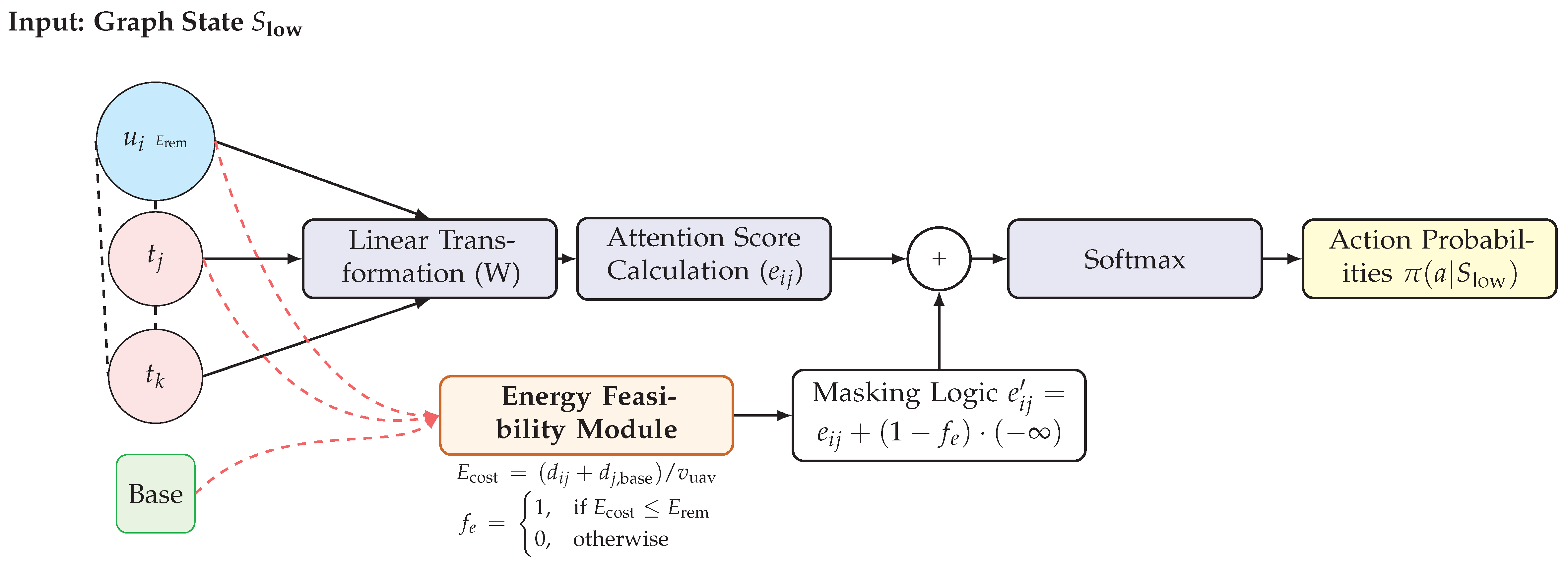
The core of the low-level policy is the proposed Energy-Aware Graph Attention Network, the architecture of which is shown in Figure 4. This network is designed to select the next task to visit by computing an attention-based probability distribution over all feasible successor nodes.

A standard Graph Attention Network (GAT) [40] computes the attention coefficient $e_{ij}$ between a query node i (the UAV’s current location) and a key node j (a candidate next task) as

$$e_{ij}=a(\mathbf{W}{\mathbf{h}}_i,\mathbf{W}{\mathbf{h}}_j)$$

(5)

where $\mathbf{W}$ is a learnable linear transformation, and a is a shared attention mechanism (e.g., a single-layer feed-forward network). The coefficients are then normalized using a softmax function to obtain the attention weights ${\alpha }_{ij}$.

The primary innovation of the Ea-GAT lies in the integration of an energy feasibility model directly into this attention mechanism. An energy feasibility function, $f_e(i,j)$, is introduced to modulate the attention scores. This function calculates the estimated energy cost $E_{\cos \mathrm{t}}(i,j)$ for the UAV to travel from its current location i to a candidate task j and subsequently return to the final destination base ${\mathbf{p}}_{\mathrm{base}}^{\mathrm{end}}$:

$$E_{\mathrm{cost}}(i,j)={\displaystyle \frac{\parallel {\mathbf{p}}_j-{\mathbf{p}}_i\parallel +\parallel {\mathbf{p}}_{\mathrm{base}}^{\mathrm{end}}-{\mathbf{p}}_j\parallel }{v_{\mathrm{uav}}}}$$

(6)

The feasibility function $f_e(i,j)$ then returns a value indicating whether this path segment is viable given the UAV’s remaining energy $E_{\mathrm{rem}}\left(i\right)$:

$$f_e(i,j)=\left\{\begin{array}{cc}1,\hfill & \mathrm{if}{E}_{\mathrm{cost}}(i,j)\le E_{\mathrm{rem}}\left(i\right)\hfill \\ 0,\hfill & \mathrm{otherwise}\hfill \end{array}\right.$$

(7)

A hard-gating function is used here for clarity, though a soft, differentiable version (e.g., using a sigmoid) can be employed in practice. The original attention coefficients $e_{ij}$ are then masked by this feasibility value before normalization. The masked coefficient $e_{ij}^{\prime }$ is computed as

$$e_{ij}^{\prime }=e_{ij}+(1-f_e(i,j))·(-\infty )$$

(8)

Applying the softmax function to these masked coefficients effectively assigns zero probability to any energy-infeasible actions, ensuring that only viable tasks are considered for the next step. This end-to-end approach guarantees that all generated paths are inherently feasible with respect to the UAV’s endurance.

3.2.3. Intent-Driven Reward Shaping

The final output of the Ea-GAT is a probability distribution over all feasible next tasks. An action is sampled from this distribution to select the next destination. The rewards, $R_{\mathrm{low}}$, used to train this policy are shaped by the intent vector $\mathbf{z}=(z_1,z_2,z_3)$ received from the meta-controller. The reward function is a linear combination of sub-rewards:

$$R_{\mathrm{low}}=z_1{R}_{\mathrm{speed}}+z_2{R}_{\mathrm{coverage}}+z_3{R}_{\mathrm{safety}}+R_{\mathrm{terminal}}$$

(9)

where $R_{\mathrm{speed}}$ is a negative reward proportional to the distance traveled, $R_{\mathrm{coverage}}$ is a positive reward for visiting a new task, $R_{\mathrm{safety}}$ is a penalty for flying close to hazards, and $R_{\mathrm{terminal}}$ is a large positive or negative reward for successfully completing the sortie or failing (e.g., due to energy depletion), respectively. This mechanism allows the low-level agent to adapt its routing behavior to align with the current high-level strategy.

3.3. Training Procedure

The H-DRL framework is trained in an end-to-end, alternating fashion. The training process cycles through experience collection and network updates. During experience collection, the high-level policy first selects a base location ${\mathbf{p}}_{\mathrm{next}}$ and an intent vector $\mathbf{z}$. Subsequently, the low-level policy, conditioned on $\mathbf{z}$, executes a full sortie by generating a sequence of actions until a terminal state is reached. The resulting trajectories, containing states, actions, and rewards for both levels, are stored in separate replay buffers.

The network parameters for both policies are updated by sampling mini-batches from their respective buffers. As specified in

Table 1. Hyperparameters for the DRL agent training.

Hyperparameter	Value	Description
DRL Algorithm	PPO
Learning Rate ($\alpha$)	3 × 10−4	For both actor and critic networks
Discount Factor ($\gamma$)	0.99	For advantage estimation
PPO Epsilon ($ϵ$)	0.2	Clipping parameter
GAE Lambda ($\lambda$)	0.95	For Generalized Advantage Estimation
Number of Epochs	10	Number of optimization epochs per update
Minibatch Size	128	Size of mini-batches for SGD
Optimizer	Adam
High-level Update Freq. ($U_{\mathrm{meta}}$)	10	Update meta-controller every 10 episodes
Low-level Update Freq. ($U_{\mathrm{low}}$)	2	Update controller every 2 episodes

, the low-level policy is updated more frequently (every $U_{\mathrm{low}}=2$ episodes) than the high-level policy (every $U_{\mathrm{meta}}=10$ episodes). This difference in update frequency is a key aspect of hierarchical training: the low-level controller requires more frequent updates to quickly master the fine-grained, tactical routing task under various strategic intents, while the high-level meta-controller learns from the aggregated outcomes of multiple low-level episodes, allowing it to focus on the slower, long-horizon strategic deployment policy. The actor–critic networks for both levels are trained using the PPO algorithm with the Adam optimizer [41]. This alternating training scheme ensures that both policies co-evolve and adapt to each other, leading to a robust and globally coordinated solution. The detailed training procedure is outlined in Algorithm 1.

Algorithm 1 Training Algorithm for the H-DRL Framework

1: Initialize high-level policy network ${\pi }_{\mathrm{meta}}\left({\theta }_{\mathrm{meta}}\right)$ and critic $V_{\mathrm{meta}}\left({\varphi }_{\mathrm{meta}}\right)$ 2: Initialize low-level policy network ${\pi }_{\mathrm{low}}\left({\theta }_{\mathrm{low}}\right)$ and critic $V_{\mathrm{low}}\left({\varphi }_{\mathrm{low}}\right)$ 3: Initialize replay buffers ${\mathcal{D}}_{\mathrm{meta}}$ and ${\mathcal{D}}_{\mathrm{low}}$ 4: for episode = 1 to $N_{\mathrm{episodes}}$ do 5:    Get initial global state $S_{\mathrm{meta}}$ 6:    // — High-level Decision Making — 7:    Select high-level action $A_{\mathrm{meta}}=(l,\mathbf{z})\sim {\pi }_{\mathrm{meta}}\left(S_{\mathrm{meta}}\right)$ 8:    Execute base relocation to location l, incur cost $C_{\mathrm{deployment}}$ 9:    Initialize cumulative low-level reward $R_{\mathrm{cumulative}\_\mathrm{low}}\leftarrow 0$ 10:    for sortie = 1 to $N_{\mathrm{sorties}}$ do 11:      Get initial local state $S_{\mathrm{low}}$ for a UAV at location l 12:      Initialize trajectory buffer ${\tau }_{\mathrm{low}}$ 13:      while $S_{\mathrm{low}}$ is not terminal do 14:         // — Low-level Path Planning — 15:         Select low-level action $a_{\mathrm{low}}\sim {\pi }_{\mathrm{low}}\left(S_{\mathrm{low}}\right)$ 16:         Execute action $a_{\mathrm{low}}$, observe next state $S_{\mathrm{low}}^{\prime }$ and reward $R_{\mathrm{low}}$ 17:         Store $(S_{\mathrm{low}},a_{\mathrm{low}},R_{\mathrm{low}},S_{\mathrm{low}}^{\prime })$ in ${\tau }_{\mathrm{low}}$ 18:         $S_{\mathrm{low}}\leftarrow S_{\mathrm{low}}^{\prime }$ 19:         $R_{\mathrm{cumulative}\_\mathrm{low}}\leftarrow R_{\mathrm{cumulative}\_\mathrm{low}}+R_{\mathrm{low}}$ 20:      end while 21:      Store trajectory ${\tau }_{\mathrm{low}}$ in ${\mathcal{D}}_{\mathrm{low}}$ 22:    end for 23:    // — High-level Reward Calculation and Storage — 24:    Calculate $R_{\mathrm{performance}}$ and $R_{\mathrm{consistency}}$ from the executed sorties 25:    $R_{\mathrm{meta}}\leftarrow w_{\mathrm{perf}}{R}_{\mathrm{performance}}+w_{\mathrm{consist}}{R}_{\mathrm{consistency}}-w_{\mathrm{dep}}{C}_{\mathrm{deployment}}$ 26:    Get next global state $S_{\mathrm{meta}}^{\prime }$ 27:    Store $(S_{\mathrm{meta}},A_{\mathrm{meta}},R_{\mathrm{meta}},S_{\mathrm{meta}}^{\prime })$ in ${\mathcal{D}}_{\mathrm{meta}}$ 28:    // — Network Updates — 29:    if episode mod $U_{\mathrm{low}}==0$ then 30:      Sample mini-batch from ${\mathcal{D}}_{\mathrm{low}}$ and update ${\theta }_{\mathrm{low}},{\varphi }_{\mathrm{low}}$ using PPO 31:    end if 32:    if episode mod $U_{\mathrm{meta}}==0$ then 33:      Sample mini-batch from ${\mathcal{D}}_{\mathrm{meta}}$ and update ${\theta }_{\mathrm{meta}},{\varphi }_{\mathrm{meta}}$ using PPO 34:    end if 35: end for

4. Experiments and Results

This section presents a series of comprehensive experiments designed to evaluate the performance of the proposed H-DRL framework. The evaluation is conducted in two stages: first, a set of extensive simulation experiments are performed to compare the framework against several baseline methods under various scenarios; second, a physical experiment is conducted to validate the feasibility and practical advantages of the proposed approach in a real-world setting.

4.1. Experimental Setup

4.1.1. Simulation Environment

All simulation experiments were conducted in a custom-built environment developed in Python 3.8, utilizing libraries such as NumPy for numerical operations and PyTorch for implementing the neural network models. The operational area is a two-dimensional square grid of size $100\times 100$ units. Inspection tasks are represented by points with coordinates randomly sampled from a uniform distribution within this area, unless specified otherwise. For dynamic scenarios, new tasks are introduced at predefined intervals during the mission execution.

All simulation experiments were conducted in a custom-built environment developed in Python (version 3.8, Python Software Foundation, Wilmington, DE, USA). The environment utilized core scientific computing libraries, including NumPy for numerical operations, and PyTorch (version 2.0, Meta AI, Menlo Park, CA, USA) for implementing the neural network models. The operational area is a two-dimensional square grid of size $100\times 100$ units. Inspection tasks are represented by points with coordinates randomly sampled from a uniform distribution within this area, unless specified otherwise. For dynamic scenarios, new tasks are introduced at predefined intervals during the mission execution.

4.1.2. System and Algorithm Parameters

The key parameters for the simulated UAV system are summarized in

Table 2. UAV system and environment parameters.

Parameter	Value
Operational Area Size	$100\times 100$ units
Number of UAVs (M)	3
UAV Speed ($v_{\mathrm{uav}}$)	1.0 unit/s
UAV Endurance ($E_{max}$)	40 s
Mobile Base Speed ($v_{\mathrm{base}}$)	0.5 units/s
Battery Service Time (${\tau }_b$)	5 s
Number of Static Sites (K)	5 (for static methods)
Number of Tasks (N)	20, 50, 100

. These parameters are selected to reflect realistic operational characteristics where endurance is a significant constraint. The hyperparameters used for training the proposed H-DRL framework and its variants are detailed in Table 1. These values were determined through preliminary experiments and are kept consistent across all relevant test cases to ensure a fair comparison.

4.1.3. Performance Metrics

To provide a comprehensive evaluation, the performance of all algorithms is assessed using the following metrics:

Makespan: This is the primary metric, defined as the total time elapsed from the start of the mission until the last task is completed. It provides a holistic measure of the overall mission efficiency.

Total Flight Distance: This metric is the sum of the distances traveled by all UAVs throughout the mission. It serves as a proxy for the total energy consumption and operational cost of the UAV fleet.

Base Relocation Distance: This metric measures the total distance traveled by the mobile base. It reflects the cost associated with the deployment and logistical effort of the ground support system.

Success Rate: This metric is particularly relevant for challenging dynamic scenarios. It is defined as the percentage of missions successfully completed (i.e., all tasks visited) out of a large number of independent runs. A failure may occur if the system cannot find a feasible solution within a given time limit or due to poor adaptive decisions.

4.2. Baseline Methods

To rigorously evaluate the performance of the proposed H-DRL framework, it is compared against five baseline methods. These baselines include traditional decoupled approaches, a simplified HRL variant, as well as ablated versions of our own framework, designed to isolate and verify the effectiveness of its key innovative components.

4.2.1. Static Two-Stage (S-TS)

This baseline represents a common and practical approach to the problem. It decouples the problem into two sequential stages: siting and routing. In the first stage, the K-Means clustering algorithm [42] is used to partition the task locations into K clusters. The centroid of each cluster is then designated as the location for a fixed static site. In the second stage, the tasks are assigned to their nearest site, and a state-of-the-art VRP solver, LKH-3 [43], is employed to find the optimal routes for the UAVs operating from each site to cover the assigned tasks. This method serves as a benchmark for traditional, non-learning-based optimization.

4.2.2. Two-Stage Greedy (TS-G)

This baseline represents a stronger heuristic-based approach, similar to the one used in the physical experiment. In the first stage, it determines the single best fixed location for a base by selecting the candidate site that minimizes the average distance to all task points. In the second stage, it employs a greedy routing policy: from the fixed base, a UAV is dispatched and always travels to the nearest unvisited task until its endurance limit forces it to return. This process is repeated until all tasks are covered. This baseline tests the efficacy of simple, local heuristics against our learning-based global optimization.

4.2.3. H-DRL with Naive Communication (H-DRL w/Naive Comm)

This baseline serves as a comparison to other advanced HRL methods by implementing a simpler, discrete form of inter-layer communication. In this variant, the high-level policy does not generate a continuous intent vector $\mathbf{z}$. Instead, it outputs a discrete “tactic mode” from a predefined set (e.g., {‘FASTEST_MODE’, ‘COVERAGE_MODE’}). The low-level policy then switches to a corresponding, fixed reward function based on this discrete command. This baseline is designed to test whether the continuous, fine-grained guidance provided by our intent vector offers a significant advantage over simpler, discrete forms of hierarchical control.

4.2.4. H-DRL Without Coordination (H-DRL w/o Coor)

This is the first ablated version of our proposed framework, designed to specifically evaluate the contribution of the coordinated credit assignment mechanism. In this version, the high-level policy does not output an intent vector $\mathbf{z}$. Consequently, the low-level policy is trained with a fixed reward function that uses a predefined, static weighting of the sub-rewards (e.g., speed, coverage, safety). By comparing our full framework to this baseline, the benefits of the dynamic, intent-driven guidance can be quantified.

4.2.5. H-DRL with Standard GAT (H-DRL w/GAT)

This second ablated version is designed to verify the effectiveness of the Ea-GAT. In this baseline, the low-level policy’s architecture is replaced with a standard Graph Attention Network (GAT) that does not have the built-in energy feasibility module. To handle the endurance constraint, this version relies solely on a large negative reward (penalty) for sorties that violate the energy limit. This comparison will demonstrate the superiority of the proposed end-to-end feasibility mechanism over traditional penalty-based reward shaping.

4.3. Simulation Results and Analysis

This section presents the results of the simulation experiments. The analysis is structured into three parts: first, the convergence behavior of the learning-based methods is examined; second, the performance of all algorithms is compared in static scenarios of varying scales; finally, the adaptability and robustness of the methods are evaluated in a dynamic scenario.

4.3.1. Convergence Analysis

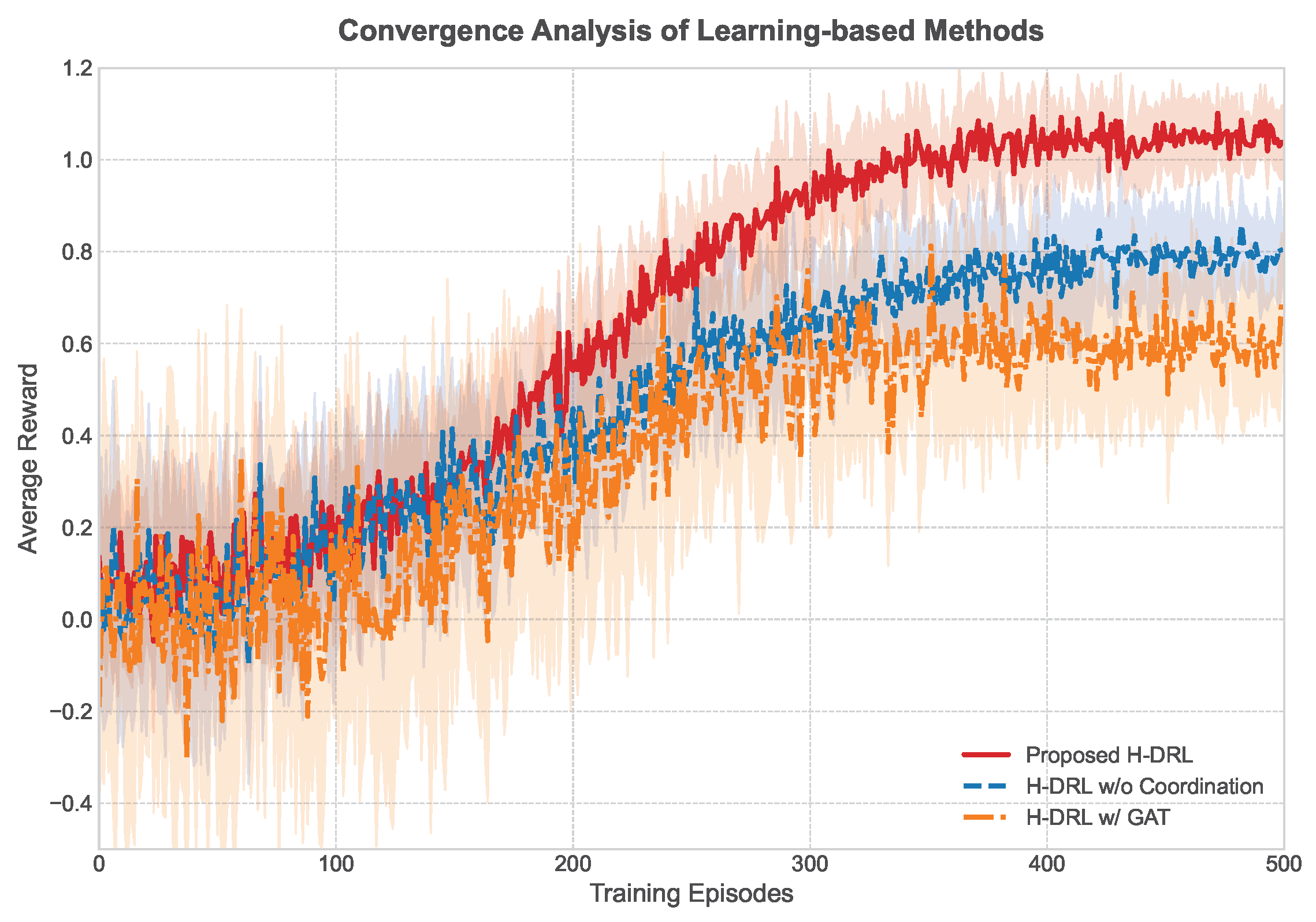
The learning curves for the proposed H-DRL framework and its two ablated versions (H-DRL w/o Coor and H-DRL w/GAT) are presented in Figure 5. The curves plot the average mission reward as a function of training episodes.

As observed in the figure, the proposed full H-DRL framework demonstrates superior convergence properties. It achieves a higher final reward and converges faster than both ablated baselines. The H-DRL w/o Coor variant learns significantly slower, indicating that the intent vector and the coordinated credit assignment mechanism provide a more effective and targeted learning signal for the high-level policy. The H-DRL w/GAT variant initially learns quickly but plateaus at a lower reward level and exhibits higher variance. This suggests that relying solely on penalty-based rewards makes it difficult for the agent to consistently discover energy-feasible, high-quality policies, highlighting the stability and effectiveness of the proposed Ea-GAT architecture.

4.3.2. Performance on Static Scenarios

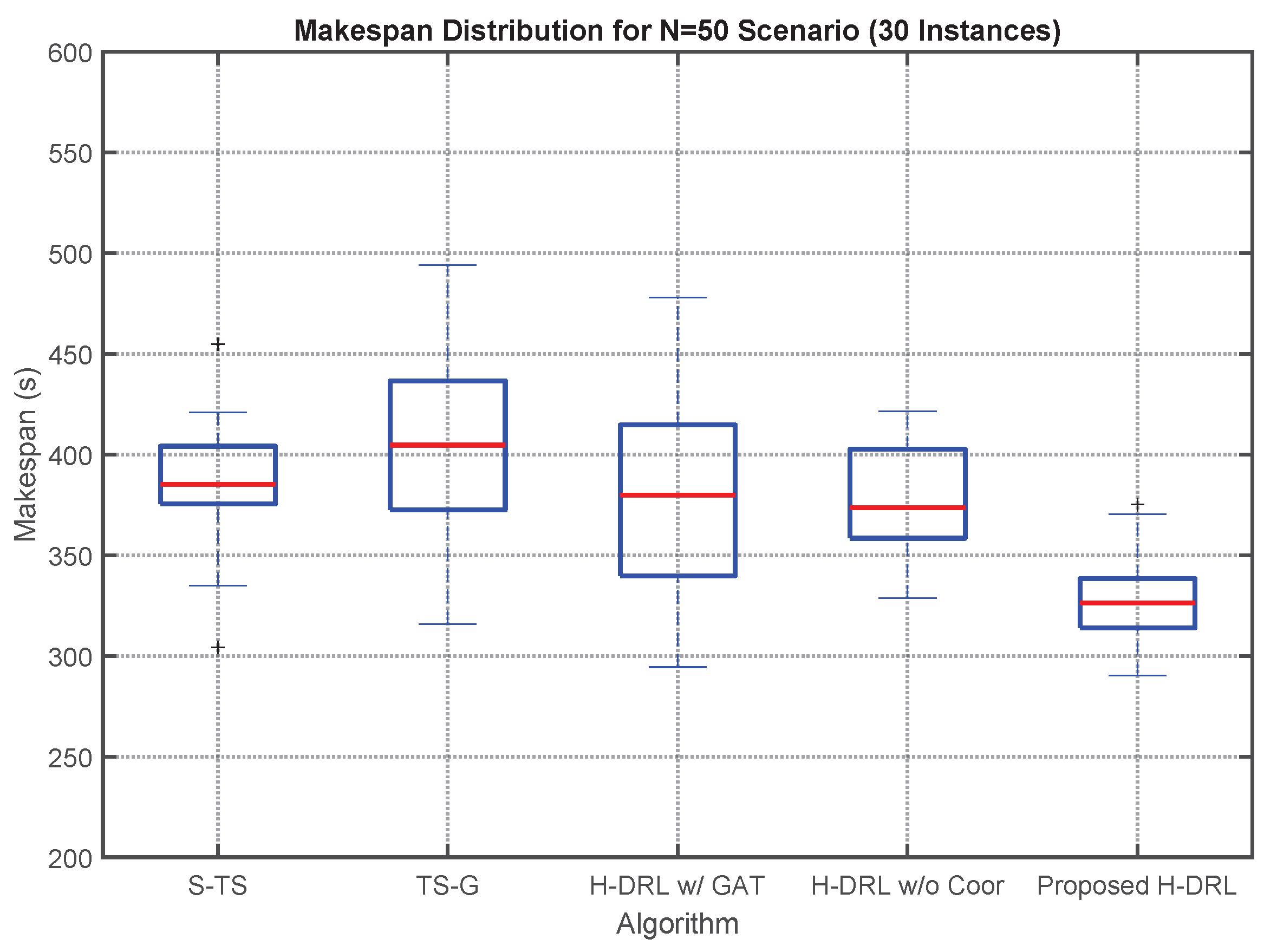
The performance of all methods was evaluated on a set of static scenarios with varying numbers of tasks (N = 20, 50, and 100). For each scenario size, 30 instances with randomly generated task locations were tested, and the average results are summarized in

Table 3. Performance comparison on static scenarios of varying scales.

	Makespan (s)			Total Flight Distance (Units)
Method	N = 20	N = 50	N = 100	N = 20	N = 50	N = 100
S-TS	150.2	380.5	850.1	250.6	650.8	1400.2
TS-G	165.8	410.2	910.7	280.1	710.3	1550.9
H-DRL w/Naive Comm	132.5	351.6	795.3	225.8	610.2	1335.1
H-DRL w/GAT	145.5	395.1	—	240.3	690.4	—
H-DRL w/o Coor	138.1	360.4	810.3	230.5	620.1	1350.6
Proposed H-DRL	125.6	330.9	750.4	210.2	580.7	1280.1

. Figure 6 provides a more detailed view of the makespan distribution for the N = 50 scenario.

The results consistently demonstrate the superiority of the proposed H-DRL framework across all scales. As shown in Table 3, our method achieves the lowest makespan in all scenarios. Compared to the traditional S-TS method, our framework shows an average improvement of 15% in makespan. This is attributed to the joint optimization of siting and routing, which allows the mobile base to be positioned more strategically than the fixed centroids determined by K-Means.

Against the heuristic-based TS-G method, our approach also yields significant gains. While TS-G is computationally efficient, its greedy nature often leads to myopic decisions, resulting in inefficient routes in the long run. The learning-based approach of H-DRL is capable of discovering more globally optimal strategies.

The comparison with the ablated versions further validates our design choices. H-DRL w/o Coor performs worse than the full framework, confirming that the intelligent guidance from the intent vector is crucial for achieving high performance. The H-DRL w/GAT struggles significantly, especially on larger instances, often failing to find feasible solutions or producing very long paths, which underscores the importance of the Ea-GAT’s endogenous constraint handling.

4.3.3. Performance on a Dynamic Scenario

To evaluate the framework’s adaptability, a dynamic scenario was designed. The mission starts with 40 initial tasks. After 200 s of mission time, 10 new, high-priority tasks are unexpectedly added to a specific quadrant of the map.

Table 4. Final makespan in the dynamic scenario.

Method	Final Makespan (s)
S-TS	Not Applicable (Static)
TS-G	550.8
H-DRL w/Naive Comm	482.5
H-DRL w/o Coor	490.2
Proposed H-DRL	465.1

compares the final makespan of the methods that can handle dynamic events.

The results highlight the significant advantage of the proposed H-DRL framework in dynamic environments. Upon the arrival of new tasks, the meta-controller of our H-DRL framework can re-evaluate the global state and make a proactive decision to relocate the mobile base to better serve the new cluster of tasks. This adaptability leads to a substantially lower final makespan compared to the TS-G method, which reacts more slowly, and the non-adaptive S-TS method, which is unable to adjust its pre-planned sites and routes at all.

4.3.4. Performance on a Scenario with Priority Changes

To further investigate the framework’s adaptability to diverse uncertainties, a scenario involving dynamic task priority changes was designed. The mission starts with 50 tasks of uniform priority (${\rho }_i=1$). At a mission time of 150 s, all uncompleted tasks within a predefined quadrant of the map have their priorities suddenly increased tenfold (${\rho }_i=10$). This scenario tests the ability of the meta-controller to shift its strategic focus in response to changing mission objectives.

The performance is evaluated by the final makespan and, more importantly, by the average completion time of the high-priority tasks after the change event. The results are presented in

Table 5. Performance comparison in the dynamic priority change scenario.

Method	Final Makespan (s)	Avg. Completion Time of High-Priority Tasks (s)
TS-G	425.6	310.2
H-DRL w/Naive Comm	385.7	278.4
H-DRL w/o Coor	390.1	285.5
Proposed H-DRL	380.4	255.8

.

The proposed H-DRL framework demonstrates a clear advantage in this scenario. Its meta-controller, observing the change in the priority distribution on its state input map, proactively issues new intents and, if necessary, relocates the mobile base to expedite the servicing of the now-critical tasks. This results in a significantly lower average completion time for high-priority tasks. The TS-G baseline, guided only by proximity, continues to service nearby low-priority tasks, failing to adapt its strategy to the new urgency. This experiment underscores the importance of a global, priority-aware strategic layer for effective decision-making in complex, evolving environments.

4.3.5. Case Study I: Strategy in a Static Scenario

To visually illustrate the fundamental strategic differences in a static environment, Figure 7 provides a comparison for a representative N = 50 instance. The figure contrasts the solution generated by the proposed H-DRL framework against the S-TS baseline.

As depicted in Figure 7a, the S-TS method is constrained by its fixed, centrally-located sites, which are determined a priori by clustering. This static placement forces UAVs to undertake numerous long-haul flights to service tasks located on the periphery of the map, resulting in significant unproductive transit time. In stark contrast, Figure 7b shows the behavior of the proposed H-DRL framework. The mobile base dynamically repositions itself multiple times throughout the mission, effectively “chasing” the dense clusters of tasks. This strategic deployment allows UAVs to be launched from optimal proximity, significantly reducing the average length of each sortie. This case study visually confirms the substantial benefits of a tightly coupled, dynamic siting and routing strategy even in static environments.

4.3.6. Case Study II: Adaptation in a Dynamic Scenario

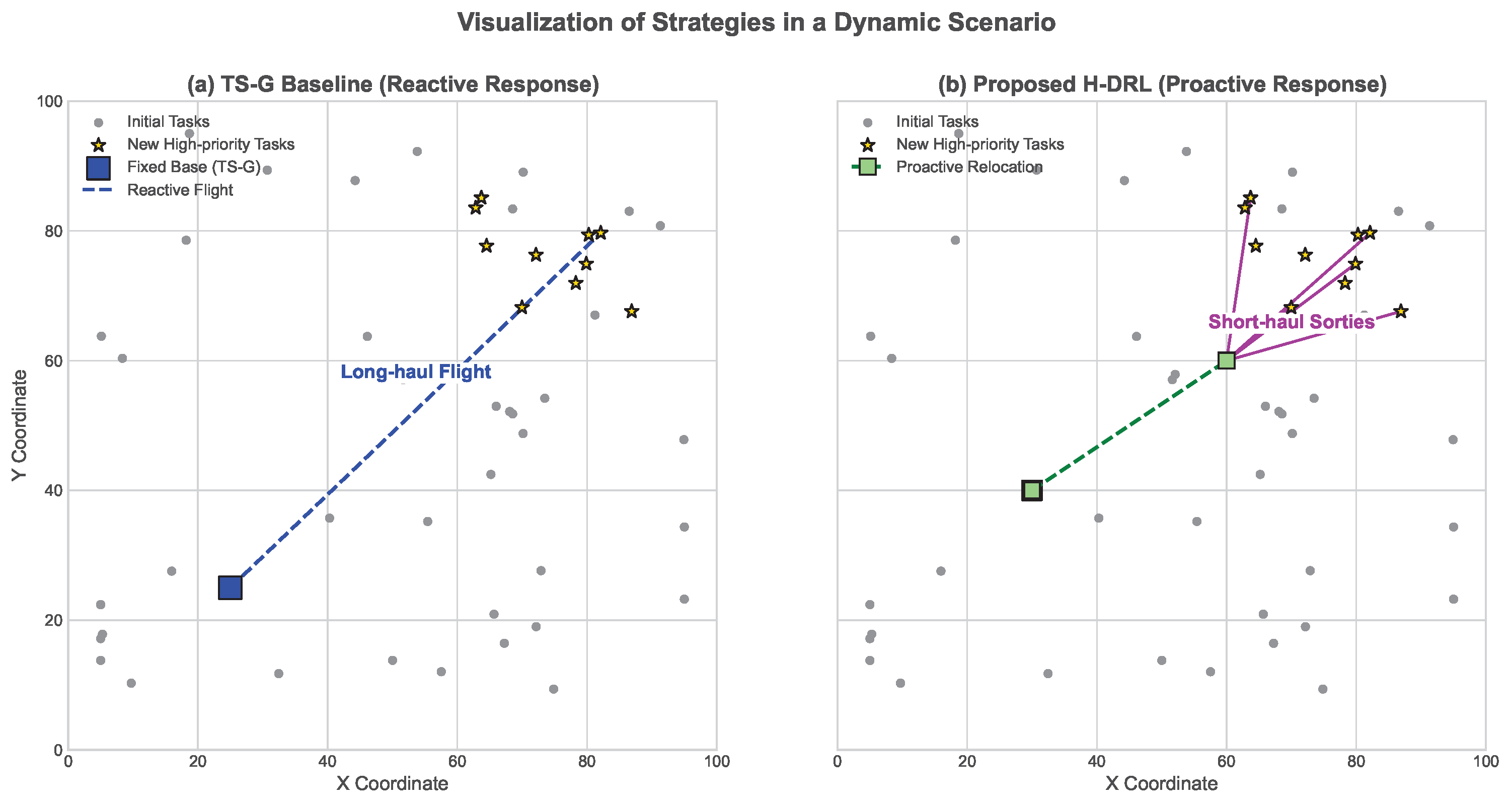
To provide an intuitive understanding of the framework’s adaptability, Figure 8 visualizes the strategic responses in the dynamic scenario where new tasks emerge mid-mission. The figure compares the proposed H-DRL framework with the reactive TS-G baseline.

Figure 8a depicts the critical moments after 10 new high-priority tasks (highlighted in yellow) appear in the top-right quadrant. The TS-G baseline, being purely reactive and tied to its pre-determined optimal fixed base, is forced to dispatch a UAV on a long-haul flight across the map to address the new tasks. This results in a significant response delay and inefficient path. In contrast, the meta-controller of the proposed H-DRL framework, shown in Figure 8b, demonstrates true adaptability. Upon detecting the change in the global state, it makes a proactive decision to relocate the mobile base towards the new task cluster. This strategic repositioning enables the subsequent launch of UAVs on short, efficient sorties to rapidly service the emergent high-priority tasks. This case study powerfully illustrates the advantage of a proactive, learning-based deployment strategy over simple reactive heuristics in dynamic environments.

4.4. Physical Experiment Validation

To bridge the gap between simulation and real-world application, a physical experiment was conducted. It is important to note that the primary goal of this experiment was not to perform an exhaustive statistical analysis or to demonstrate large-scale scalability. Instead, it was designed as a proof-of-concept validation. The objectives were twofold: (1) to confirm the feasibility of executing the trajectories generated by the framework on a physical UAV platform and (2) to provide a tangible, qualitative demonstration of the core strategic advantage of the coordinated approach over a traditional baseline in a controlled setting.

4.4.1. Experimental Setup

The experiment was performed in an indoor laboratory space of approximately $3\times 5\times 1.5$ m. The UAV platform used was a custom-built quadrotor equipped with an onboard flight controller capable of autonomous waypoint navigation. The physical layout of the experiment is shown in Figure 9.

The scenario was designed to directly test the framework’s ability to perform coordinated siting and routing. As detailed in

Table 6. Coordinates of sites and tasks in the physical experiment.

Point	X (m)	Y (m)	Z (m)
Site A (Start)	0.5	0.5	0.02
Site B (Optimal End)	1.5	4.5	0.02
Site C (Suboptimal End)	2.5	1.0	0.02
Task T1	0.5	3.5	1.0
Task T2	2.5	3.5	1.2
Task T3	0.5	4.5	0.8
Task T4	2.5	4.5	0.7

, one fixed starting site (A) and two candidate landing sites (B and C) were marked on the ground, along with four task points (T1–T4) marked at specified heights. The tasks were intentionally clustered in the far end of the workspace, near the optimal candidate landing site B, creating a clear strategic choice.

A critical state characteristic for the low-level policy is the remaining energy, $E_{\mathrm{rem}}$. In the physical experiment, real-time battery voltage monitoring was not employed. Instead, a linear energy consumption model based on flight time was used for decision-making within the algorithm. The remaining endurance at any given time t was estimated as $E_{\mathrm{rem}}\left(t\right)=E_{max}-t_{\mathrm{flight}}$, where $E_{max}$ was set to a conservative value based on the platform’s known flight capabilities, and $t_{\mathrm{flight}}$ is the elapsed time since the start of the current sortie. While this is a simplified model, it is sufficient for validating the waypoint navigation feasibility and the high-level strategic decision-making of the framework.

4.4.2. Procedure and Results

The experiment consisted of two trials to compare the strategies generated by the proposed H-DRL framework and the Two-Stage Greedy (TS-G) baseline. For each trial, the algorithm first computed a mission plan based on the coordinates in Table 6. This plan was then converted into a sequence of waypoints and uploaded to the UAV’s flight controller for autonomous execution. The mission time was recorded from takeoff to landing.

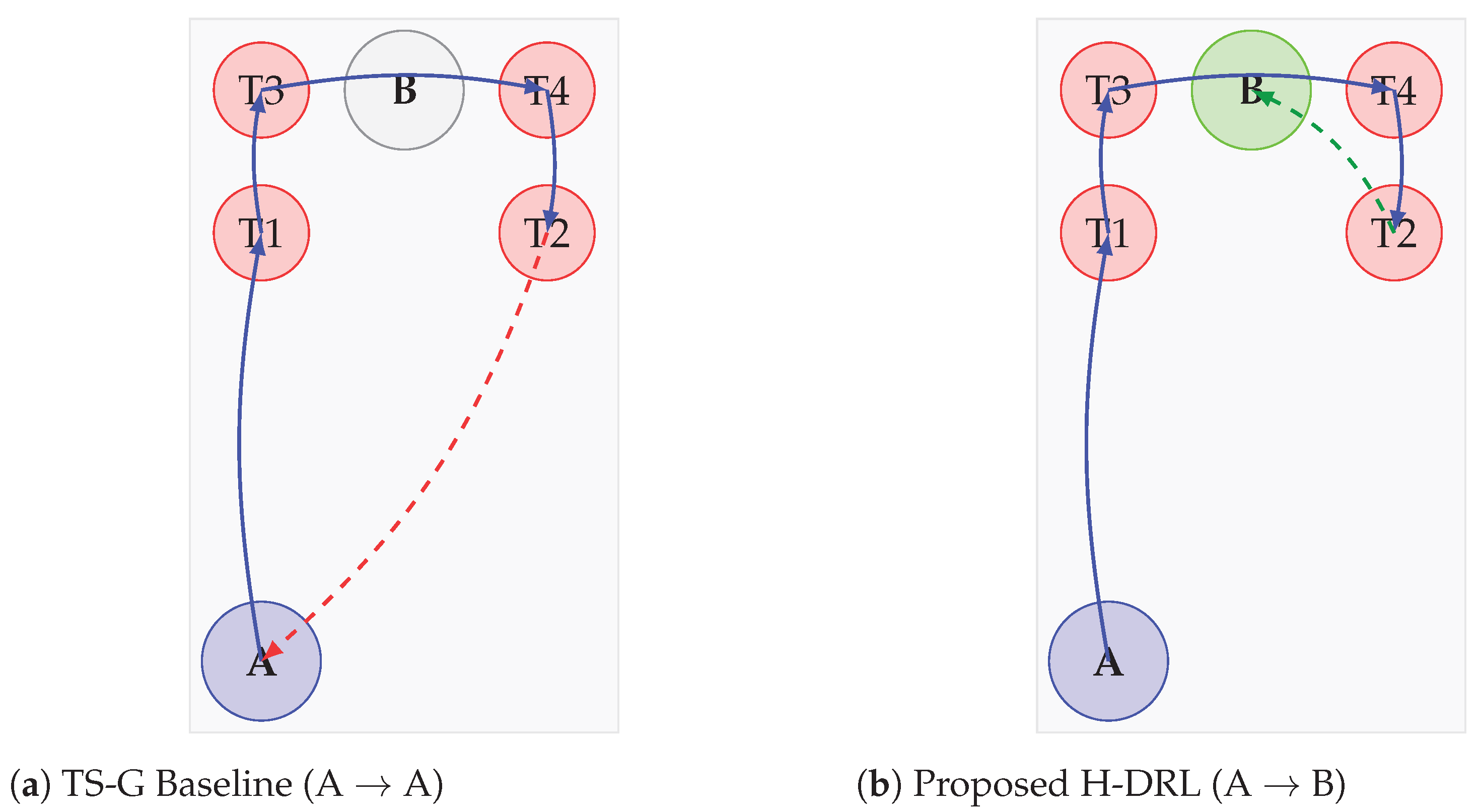
The conceptual difference between the two executed paths is visualized in Figure 10, and the quantitative results are summarized in

Table 7. Quantitative results of the physical experiment.

Metric	TS-G Baseline	Proposed H-DRL
Deployment Strategy	A → A (Fixed)	A → B (Dynamic)
Planned Path Length (m)	11.15	9.14 (−18.0%)
Actual Mission Time (s)	32.5	27.2 (−16.3%)

. The proposed H-DRL framework, performing a global optimization, generated a dynamic ‘A -> B’ deployment strategy, which resulted in a shorter overall path. The TS-G baseline, constrained to a fixed-base strategy, planned a path starting from and returning to A, necessitating a long final return leg.

The successful completion of both autonomous flights confirmed the feasibility of the generated trajectories. The quantitative results in Table 7 clearly demonstrate the superiority of the proposed method. By intelligently selecting the landing site, the H-DRL framework reduced the total path length by 18.0% and the actual measured mission time by a significant margin of 16.3%. This provides direct physical evidence of the framework’s ability to achieve more efficient global solutions through its coordinated siting and routing strategy.

5. Conclusions

This paper has addressed the central research question of whether a hierarchical learning structure can effectively solve the joint UAV siting and routing problem. To this end, a novel Hierarchical Reinforcement Learning (H-DRL) framework was proposed. This framework effectively decouples the problem into a high-level strategic deployment policy and a low-level tactical routing policy. Its core innovations—a coordinated credit assignment mechanism using a learned intent vector, and an Energy-Aware Graph Attention Network (Ea-GAT) that endogenously handles UAV endurance constraints—proved crucial for achieving a robust and globally coordinated solution.

The comprehensive experimental results confirm the hypothesis that a hierarchical approach is superior for this problem. The proposed framework was shown to significantly outperform traditional optimization and heuristic baselines. For instance, in static scenarios with 50 tasks, the H-DRL framework reduced the mission makespan by an average of 13.0% compared to the Static Two-Stage (S-TS) method. The value of both the inter-layer coordination and the intra-policy constraint handling was confirmed through rigorous ablation studies. Furthermore, a physical experiment with a custom-built quadrotor validated the real-world feasibility of the generated trajectories, showing that the intelligent deployment strategy reduced the actual mission time by 16.3% against the greedy baseline.

While this work provides a robust solution for automating complex UAV operations, several avenues for future research remain open. A key limitation of the current framework is its reliance on the assumption of perfect global information for the meta-controller’s state. Real-world scenarios often involve communication delays and partial observability, which presents a significant challenge. Future work should therefore explore the integration of Partially Observable MDP (POMDP) formalisms. The physical validation, while demonstrating feasibility, was limited to a small-scale indoor setting with single-run comparisons. Therefore, future work should focus on extensive testing in larger, more complex outdoor environments with multiple trials to enable rigorous statistical analysis of the performance differences. From a methodological perspective, the scalability and computational cost of the proposed framework present challenges for extremely large-scale problems. The training of deep hierarchical models is inherently sample-intensive, requiring significant computational resources. Future research could explore methods such as imitation learning [44] to accelerate convergence. Exploring decentralized multi-agent H-DRL frameworks [45], where coordination is achieved through local communication [33], is a promising direction for larger UAV fleets. Finally, incorporating more sophisticated, physics-based energy consumption models [46] and extending to full 3D environments are also important next steps toward real-world deployment. In conclusion, this research not only offers a practical solution for a challenging robotics problem but also contributes valuable insights into the design of intelligent, hierarchical control systems for real-world logistics and critical infrastructure management.