Article

Nine-Probe Third-Order Matrix System for Precise Flatness Error Detection

by
Hua Liu
1,2,
Jihong Chen
1,
Zexin Peng
2,
Han Ye
3,
Yubin Huang
1,* and
Xinyu Liu
2
1
School of Mechanical Science and Engineering, Huazhong University of Science and Technology, Wuhan 430074, China
2
Jiangxi JUST Machine Tool Co., Ltd., No.1618 Jinsha 2nd Road, Xiaolan Development Zone, Nanchang 330200, China
3
School of Mechanical and Electrical Engineering, Nanchang University, Nanchang 330031, China
*
Author to whom correspondence should be addressed.
Machines 2025, 13(9), 856; https://doi.org/10.3390/machines13090856
Submission received: 27 July 2025 / Revised: 4 September 2025 / Accepted: 8 September 2025 / Published: 16 September 2025

Abstract

Large-scale, high-density flatness measurement is critical for manufacturing reference surfaces in ultra-precision machine tools. Traditional methods exhibit degradation in both accuracy and efficiency as measurement points and area size increase. In order to overcome these limitations to meet the requirements for integrated in-process measurement and machining of structural components in ultra-precision machine tools, this paper proposes a novel nine-probe third-order matrix system that integrates the Fine Sequential Three-Point (FSTRP) method with automated scanning path planning. The system utilizes a multi-probe error separation algorithm based on the FSTRP principle, combined with real-time adaptive sampling, to decouple machine tool motion errors from intrinsic workpiece flatness deviations. This system breaks through traditional multi-probe 1D straightness measurement limitations, enabling direct 2D flatness measurement (with X/Y error decoupling), higher sampling density, and a repeatability standard deviation of 0.32 μm for large precision machine tool components. This high-efficiency, high-precision solution is particularly suitable for automated flatness inspection of large-scale components, providing a reliable metrology solution for integrated measurement-machining of flatness on precision machine tool critical components.

1. Introduction

In precision machine tool manufacturing, achieving rapid, high-density flatness measurement is critical. Current research focuses on dynamic error suppression, intelligent algorithm optimization, and large workpiece measurement. In the context of measurement data processing, Dichev uses Kalman filtering framework enhances anti-interference by separating model errors from measurement noise [1]. Huang enables efficient large-scale evaluation via coordinate-transformation-based preprocessing [2]. Shu optimizes micro-nano surface point-cloud processing through improved particle swarm optimization and hierarchical clustering [3]. Saleh quantifies environmental influences using Fizeau interferometry while eliminating back-reflection errors via surface treatment [4]. Liu’s team enhances point-cloud quality by combining genetic algorithms with gradient-boosted decision trees and rotating platforms [5]. Zhou’s spatial-transformation stitching algorithm optimizes guideway flatness with high-precision optics [6]. Miko analyzes sampling strategy impacts using regression models [7]. Yang validates laser tracker multi-station accuracy optimization [8]. Dichev proposed a Kalman filter-based algorithm for real-time correction of dynamic errors in flat surface metrology under mechanical disturbances [9]. Mathews achieves geometric error reduction via FEM-assisted correction [10].
Regarding methodologies for flatness error measurement, Su et al. attain ±0.1 μm straightness accuracy using thin-film interferometry, analyzing air-wedge phase variations with temperature-robust validation [11]. Lai et al. demonstrate 100 nm precision on concave spheres via multibody-theory error allocation [12]. Kiyono/Gao resolve multi-beam phase distortion through edge extraction in joint differential profiling [13]. Chai et al. achieve 0.08 μm deviation with flexure-hinge multi-probe error isolation [14]. Gao et al. verify sub-micron cylinder straightness using reversal-method probes [15]. Li et al. control FF-number deviations within 2.6 mm via planar-mirror laser coverage optimization [16]. Xiao et al. reach 0.072 mm uncertainty in annular flange measurement via point-cloud transformation [17]. Elmelegy/Zahwi show 50% angular error reduction with autocollimators [18]. Hwang et al. attain 0.05 μm rail straightness via integrated two-point/reversal probing [19].
Moreover, Stauffenberg et al. developed the NFM-100 planar Nano positioning machine, which maintains nanoscale trajectory deviation even at a high speed of 20 mm/s within a motion range of Ø100 mm, providing support for large-range sub-nanometer positioning in precision measurement [20]. Yang et al. proposed a multi-probe system that combines an autocollimator and laser interferometers to simultaneously measure the yaw and straightness errors of XY stages and reconstruct the reference bar mirror profile, with a measurement standard deviation of around 10 nm [21]. Manske et al. presented the NPMM-200 Nano positioning and Nano measuring machine, which achieves 20 pm resolution over a 200 mm range and establishes direct traceability to atomic clocks through frequency comb technology, breaking through the bottleneck of cross-scale sub-nanometer measurement [22].
Existing large-scale flatness measurement techniques have problems such as reduced efficiency from manual sampling, repeatability errors caused by environmental factors, and difficulties in separating machine tool motion errors from workpiece form deviations. Notably, through those traditional multi-probe systems mention above are primarily designed for one-dimensional straightness measurement—for instance, detecting the straightness of X-axis or Y-axis guideways independently. They lack the capability to characterize the full-field topography of 2D flat surfaces, often requiring error-prone “line-scan stitching” to extend single-axis data to planar areas. In contrast, the proposed 9-probe third-order matrix system, with its 3 × 3 array configuration, enables direct 2D flatness measurement via synchronized horizontal and vertical probe groups, eliminating stitching errors and realizing full-field error decoupling. These methods are unsuitable to meet integrated measurement-machining needs for critical datum surfaces of precision machine tool structural components and cannot provide micron-level accuracy or in-process form adjustment required for precision surface generation of precision machine tool.
To address these issues, this study proposes an integrated nine-probe matrix system featuring FSTRP-based multidimensional error decoupling and CNC-driven adaptive scanning. In Section 2, the mathematical modeling of error separation algorithms is detailed; in Section 3, experimental characterization of system repeatability (σ ≤ 0.63 μm) is presented; and in Section 4, performance benchmarking against electronic levels is conducted. Verification experiments demonstrate that the proposed method achieves comparable accuracy to conventional approaches while significantly outperforming in measurement efficiency and sampling density.

2. System Design and Algorithm Development

2.1. System Configuration and Measurement Principle

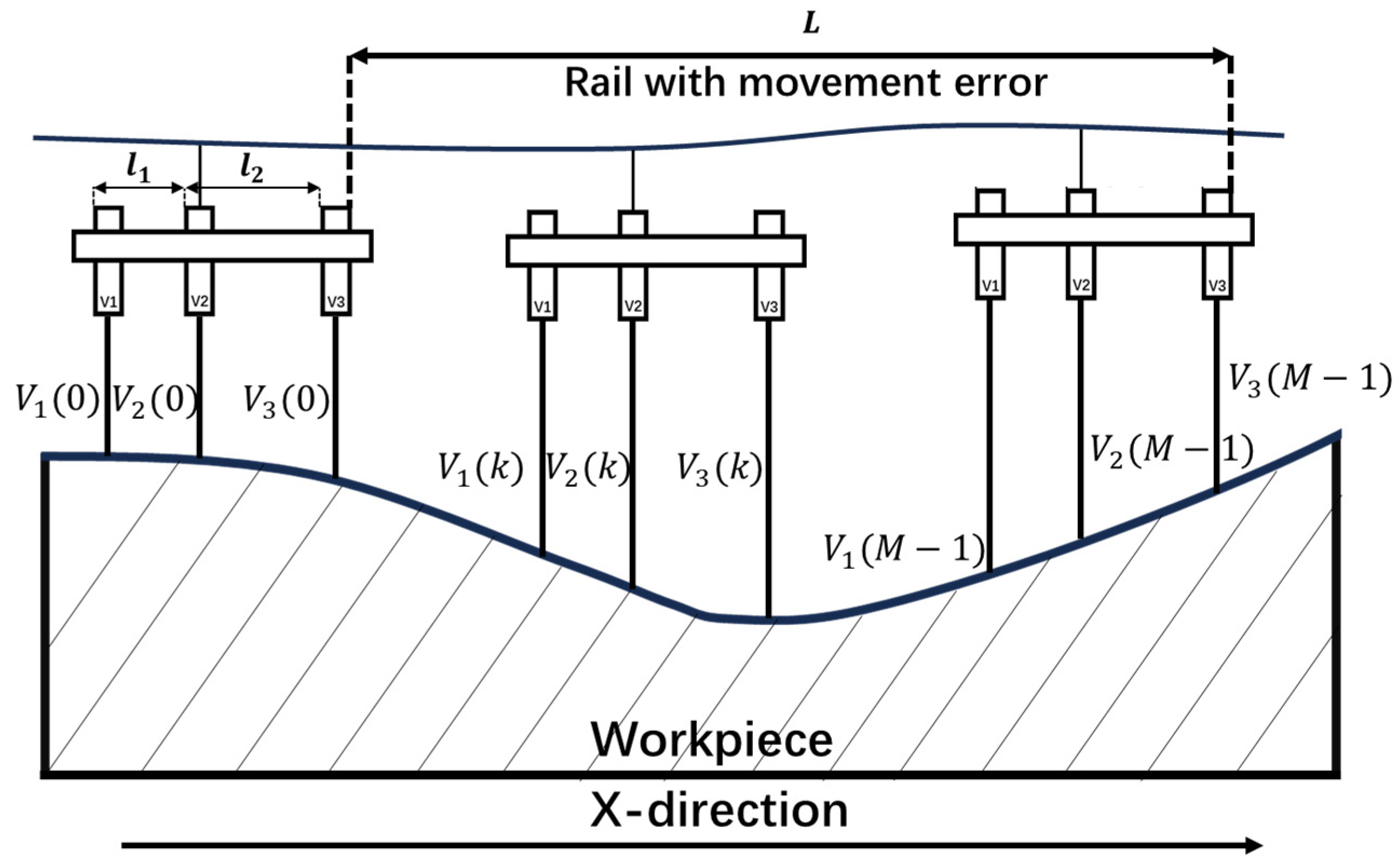
To separate measurement errors, this paper introduces the Nine Probe Third-order Matrix Error Separation method, an extension of the Fine Sequential Three-Point Method (FSTRP) error separation technique, with its prototype structure shown in Figure 1. The term ‘third-order’ refers to the 3 × 3 spatial arrangement of the nine probes (3 rows × 3 columns)—this configuration provides sufficient redundant sampling to support 2D flatness measurement.
Nine high-precision probes are instaled on the feed axis of the machine tool, scans and measures the surface error of the workpiece through a given path, and uses advanced error separation algorithms to separate the system error of the machine tool motion system from the flatness error of the workpiece itself.
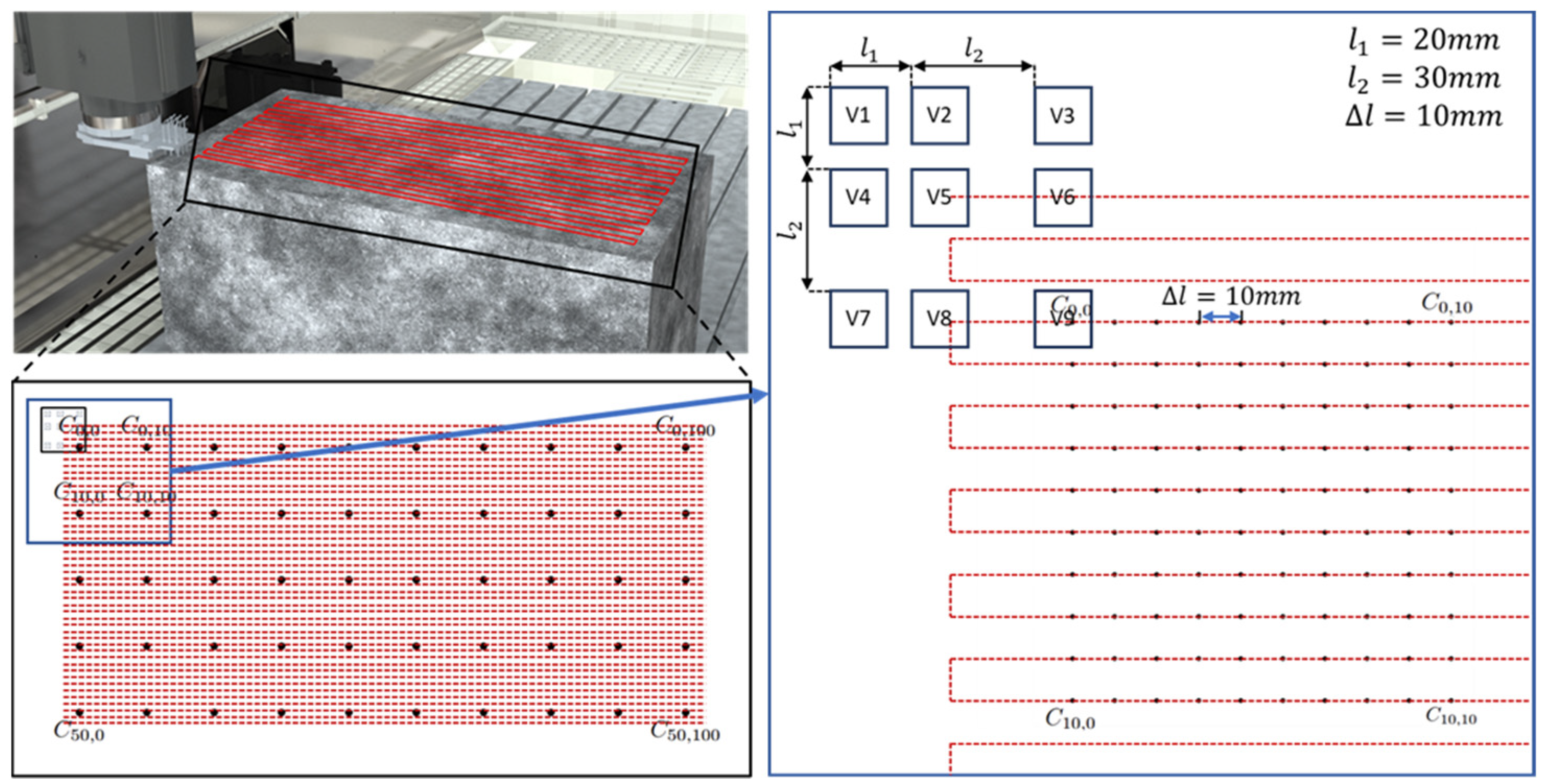
In Figure 2, V1 to V9 denote the nine probes arranged in a 3 × 3 matrix. l 1 and l 2 represent the distance between the probe, Δ l represents the sampling interval. A critical requirement is that l 1 must be an integer multiple of Δ l ( l 1 = Δ l k ,   k Z ). This condition ensures that, after a series of displacements, multiple probes will collect data at the same sampling point location.
This schematic illustrates a metrology system implementing a nine-probe third-order matrix methodology. A PC based workstation interfaces with the machine tool CNC system via a network protocol. The CNC system orchestrates the servo drives of the machine tool’s feed axes, which in turn actuate the nine probes mounted thereon. During the scanning process, the CNC system records the positional data of the feed axes while executing a predefined trajectory across the workpiece surface. The probes, affixed to the moving feed axes, collect surface topography data which is transmitted to the CNC system through a data acquisition card. The CNC system then correlates this data with the corresponding feed axis positions to compute the surface deviations of the workpiece. Subsequently, the processed information is relayed to the PC. Leveraging advanced algorithms grounded in the nine-probe third-order matrix method, systematic errors are decomposed by the PC from the flatness errors of the workpiece, thereby enabling comprehensive error analysis.
To ensure measurement validity, the following assumptions are verified based on probe specifications and calibration:
  • Probe linearity: Each high-precision capacitive probe (HD series) has a linear error ≤ 0.1% of full scale, confirmed via calibration with a Renishaw XL-80 laser interferometer;
  • Simultaneous sampling: The nine probes achieve synchronous data acquisition with a time deviation ≤ 1 ms, guaranteed by the CNC system’s 60 Hz real-time sampling module;
  • Probe position accuracy: The 3 × 3 probe matrix is calibrated via a coordinate measuring machine (CMM, accuracy ±2 μm), ensuring the distance between adjacent probes has a position error ≤ 5 μm.
Specifically, the nine probes are divided into three horizontal groups (V1-V2-V3, V4-V5-V6, V7-V8-V9) and three vertical groups (V1-V4-V7, V2-V5-V8, V3-V6-V9). During scanning, horizontal groups move along the X-axis to measure each row of the workpiece sequentially, while vertical groups move along the Y-axis to measure each column. This cross-scanning mode ensures that each sampling point C i j is measured by at least three horizontal probes and three vertical probes, generating redundant data to suppress random noise. Working principle of measurement system has been shown in Figure 3.

2.2. Error Separation Algorithm Formulation

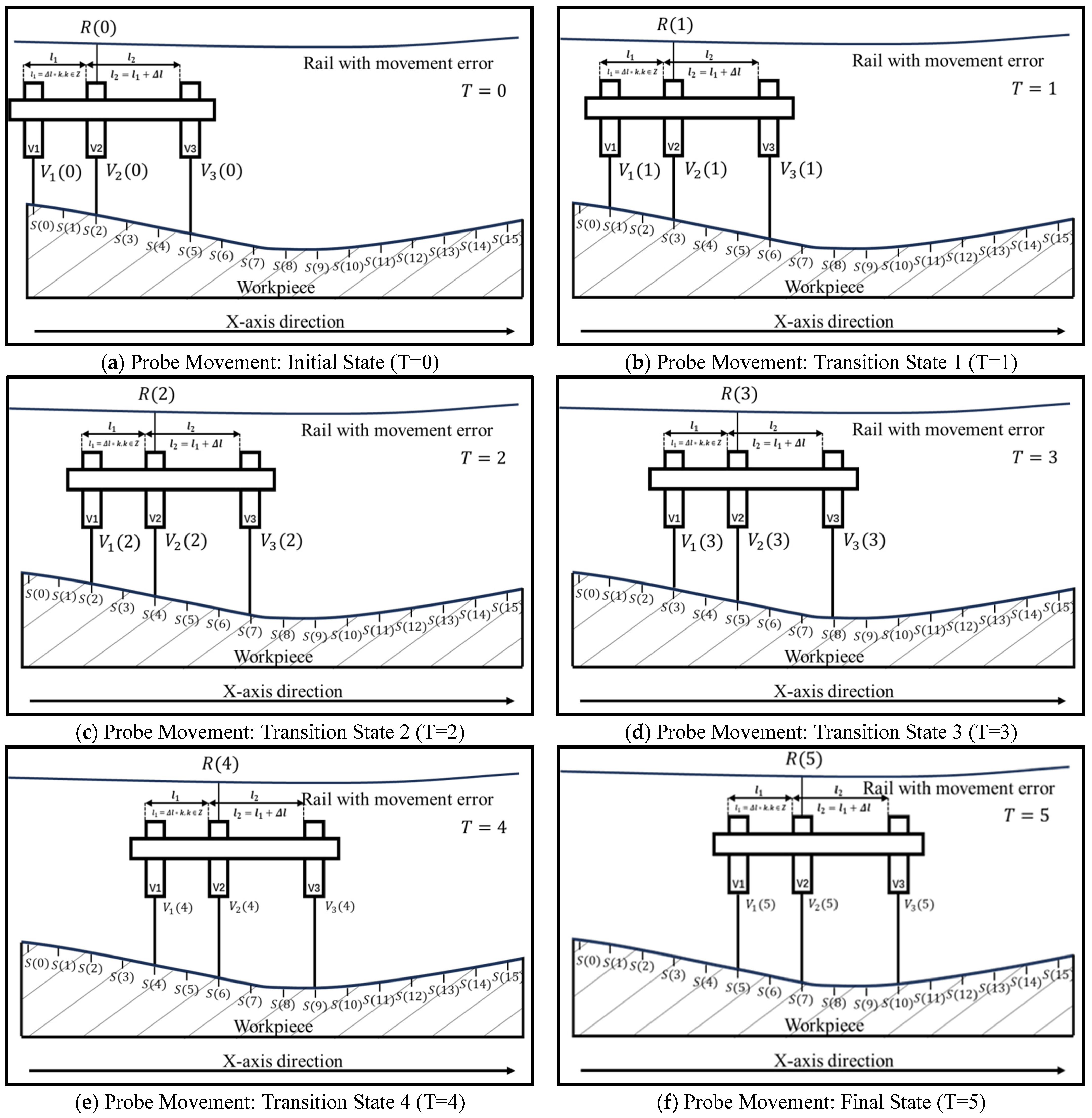
As shown in Figure 4, the measurement process and error separation principle for the X-direction probe group (V1, V2, V3) are illustrated. The relationship between l 1 , l 2 and Δ l aligns with the structural section described in Figure 2. R x denotes the motion error of the X-direction guide rail, S x represents the workpiece surface shape error, and V1 (X), V2 (X), and V3 (X) are the measurement values of probes V1, V2, and V3, respectively.
Therefore, the measurement equations of the three sensors are
V 1 x = S x + R x  
V 2 x = S x + l 1 + R x
V 3 x = S x + l 1 + l 2 + R x
Discretize Equations (1)–(3) to obtain:
V 1 k = S k +   R k  
V 2 k = S k + m 1 + R k
V 3 k = S k + m 1 + m 2 + R k
In this equation: m 1 = l 1 Δ l , m 2 = l 2 Δ l , k = x Δ l .
Base on Equations (4)–(6):
R k =   R k m 1 + ( V 1 k V 2 k m 1 )
R k = R k m 1 m 2 + ( V 1 k V 3 k m 1 m 2 )
Using Formula (7), the values of each point on the guide rail error curve with an interval of m 1 can be determined. The employment of Formula (8) facilitates the identification of values at intervals m 1 + m 2 . The intersection points of the two curves will be located at the common multiples of m 1 and m 1 + m 2 . By rotating the curves so that they align with these common multiples, the curves will coincide with the actual error curve. Utilizing Formula (8) as the basis, using Formula (7) to calculate the values at other sampling points spaced at intervals of m 1 intervals allow the sampling density to be enhanced. The workpiece’s shape error is then calculated using the Formula (4), which separates the errors.
Figure 5 provides a specific example of error separation using a probe. As illustrated in Figure 5a,c, the probe measurement values V 1 ( 2 ) and V 2 ( 0 ) denote the displacement signals measured by probes V 1 and V 2 at the position of the workpiece S ( 2 ) . By applying Formula (7):
R 2 = R 0 + ( V 1 2 V 2 0 )
the variation between guide rail positions R ( 0 ) and R ( 2 ) can be determined. Repeating this method allows the establishment of relationships between all even-spaced rail points starting from position 0 (R0, R2, and R4). Similarly, in Figure 5b,d, measuring V 1 ( 3 ) and V 2 ( 1 ) enables the derivation of the relationship between R ( 1 ) and R ( 3 ) . By extending this approach, relationships between all odd-spaced rail points starting from position 1 (R1, R3, and R5) can be established. However, the relationship between these two curves remains undefined. To bridge this gap, the values V 3 ( 0 ) and V 1 ( 5 ) , as shown in Figure 5a,f, are substituted into Formula (8):
R 5 = R 0 + ( V 1 5 V 3 0 )
By utilizing this formula, the relationship between R 0 and R 5 can be determined. This connection allows the integration of the two curves, thereby establishing a comprehensive relationship between all guide rail points from R 0 and R 5 . Assume the rail error in R 0 is 0, set it as a reference point, the error of all the other rail sampling point R k can obtain. Apply those values in Formula (4), using V 1 k = S k +   R k to calculate the workpiece error S(k).
The sampling grid distribution on the workpiece is illustrated in Figure 1. The nine-probe array executes a synchronized scan along the predefined trajectory, enabling each sampling point C i j to be interrogated from nine unique spatial positions. This multi-orientation measurement strategy facilitates redundant data acquisition for subsequent error separation.
For each horizontal probe group (e.g., V1, V2, V3), three collinear probes sequentially measure points along a common row. The acquired displacement data for each row is processed using the error separation algorithm mentioned in this chapter to separate the motion error of the X-direction guide rail R(x) and the workpiece surface shape error S(x) from the probe measurement value. Yielding the workpiece surface shape error matrix S x 1 after traversing all rows.
S x 1 = 0 S 01 S 02 S 0 N S 10 S 11 S 12 S 1 N S ( M 1 ) 0 S M 1 1 S M 1 2 S M 1 N S M 0 S M 1 S M 2 S M N
Analogous processes are applied to the remaining two horizontal probe groups, generating matrices   S x 2 and   S x 3 . Each matrix S x n ( n = 1,2 , 3 ) is an M × N array, where M denotes the number of rows and N denotes the number of sampling points per row.
For vertical measurements, three collinear probes (e.g., V1, V4, V9) sequentially measure points along each column. The same FSTRP algorithm is applied to generate column-wise error-separated matrices S y 1 , S y 2 , and S y 3 . Each matrix S y n ( n = 1,2 , 3 ) is a N × M array, transposed to align with the horizontal matrices.
The average workpiece error matrices in the X-direction S x and Y-direction S y are computed using weighted averaging:
S x = w 1 S x 1 + w 2 S x 2 + w 3 S x 3 w 1 + w 2 + w 3
S y = w 1 S y 1 + w 2 S y 2 + w 3 S y 3 w 1 + w 2 + w 3
The weights w n in Equations (10)–(12) are derived from a reliability-based normalization scheme that accounts for both systematic and random errors in each probe group’s measurements. Each probe group undergoes calibration on a certified reference flat (flatness < 0.5 μm) with 100 repeated measurements. Repeatability R n defined as the standard deviation of repeated measurements, and bias B n representing the deviation from the known reference value. Formula (12) shows the relationship between the reliability of each probe group and its repeatability ( R n ) and the deviation from the known reference value ( B n ).
R e l i a b i l i t y n = 1 R n 2 + B n 2
where lower variability and bias yield higher reliability values. The weights w n are then computed by normalizing these reliability scores by Equation (13), ensuring that more trustworthy data contributes proportionally more to the final error matrix. This approach effectively prioritizes measurements from more reliable probe groups.
w n = R e l i a b i l i t y n k = 1 3 R e l i a b i l i t y k
where weights w n are determined by the inverse of the variance matrix derived from probe calibration data. Finally, the combined flatness matrix S s is generated by fusing the X and Y error matrices:
S s = S x + S y T 2
Meanwhile, in the error separation algorithm, the drift curves between probes in the same group need to be highly consistent, so that differential operations can suppress the common mode drift component of rail errors (i.e., probe system drift). The specific method is outlined as follows: the calculation of guideway errors (Equations (7) and (8)) involves difference operations the on-probe measurements V 2 , V 3 and V 1 . When there is a drift error D in the probe, the measurement can be expressed as:
V i k = S k +   R k + D ( k )
When the probe drift curve remains highly consistent and satisfies the consistency condition D k m 1 D ( k ) , subsequent difference operation will yield:
V 2 k m 1 V 1 k = R k m 1 R k + D k m 1 D k = R k m 1 R k
Due to their approximate equality, drift errors will be eliminated during the differential operation, retaining only the variation of the guide rail error R and effectively separating the target error. Thereby improving the signal-to-noise ratio of the measurement results.

3. Experimental System Development and Uncertainty Evaluation

3.1. Experimental Setup Design and Integration

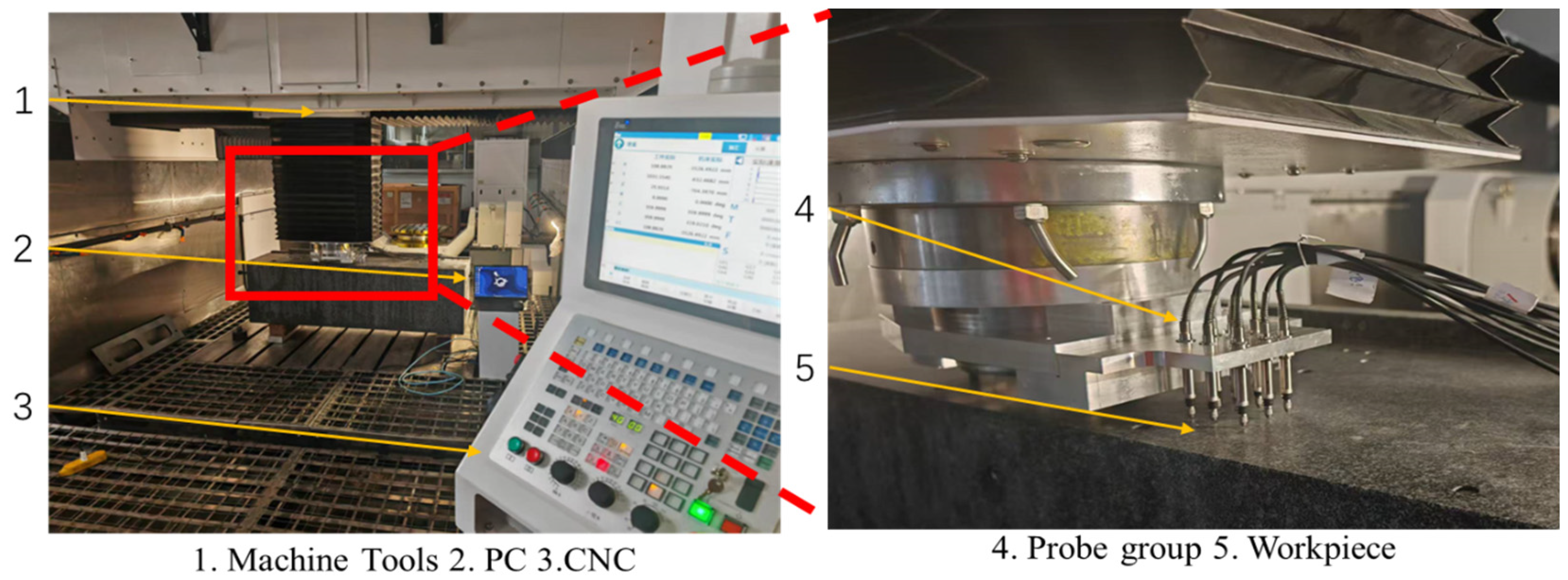
Building on the algorithm and prototype presented in the preceding chapter, an experimental system for workpiece flatness measurement was developed, as shown in Figure 6. The system is architected around a machine tool platform, integrating high-precision sensing modules, real-time data acquisition subsystems, and offline analytical software to enable precise flatness monitoring.

3.2. Machine Tool Accuracy and Repeatability Testing

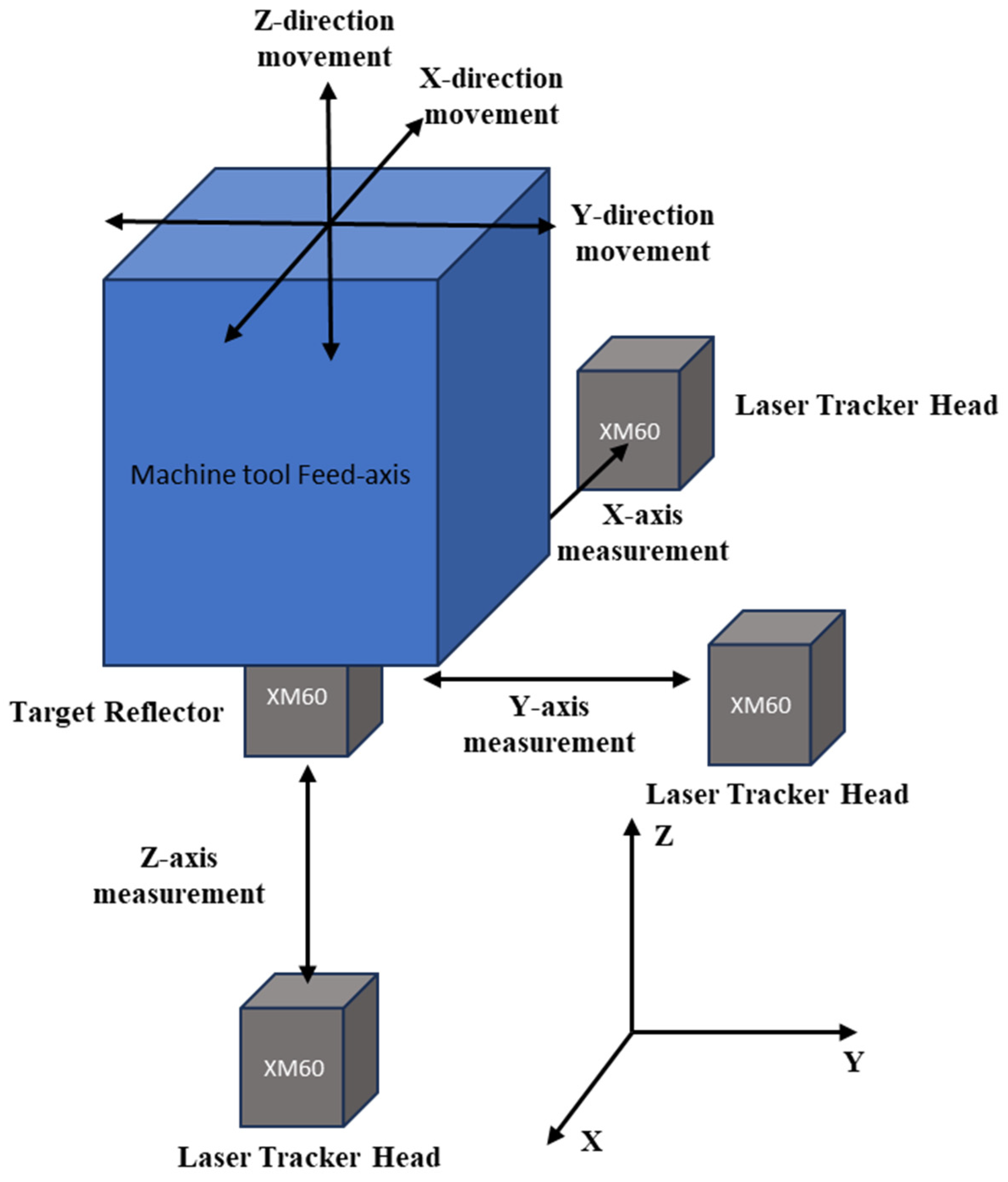
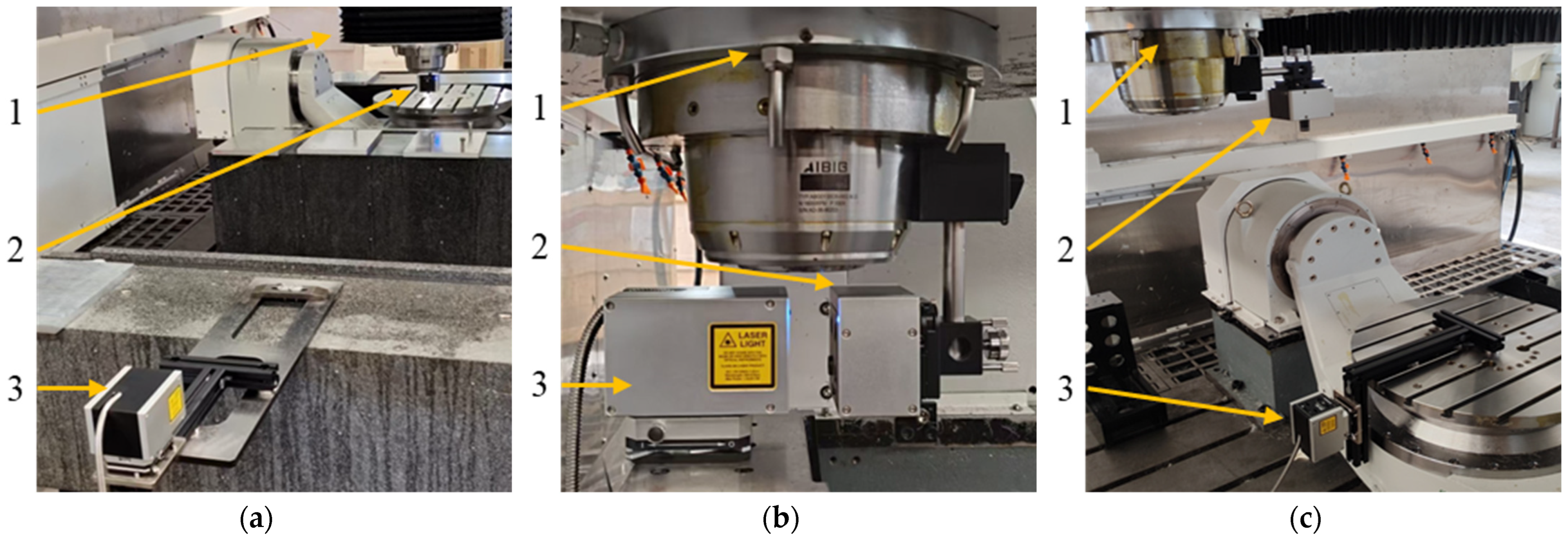
To assess the stability of experimental equipment, an integrated precision measurement-compensation test was performed on a G2040 gantry-type CNC machine using Renishaw’s XM-60 multi-axis calibrator. The XM-60 target reflector was rigidly affixed to the machine’s linear feed axis, while the laser tracker head—mounted on the machine frame in the corresponding Cartesian orientation—was optically aligned with the reflector, as shown in Figure 7. Linear positioning errors along the X, Y, and Z axes were measured by programmatically actuating the servo axes through predefined linear traverses. The experiment photo has been shown in Figure 8 and the measurement results were shown in Figure 9.
Three replicate trials of six-degree-of-freedom error measurements yielded positional error standard deviations of 0.308 μm, 0.207 μm, and 0.257 μm for the X, Y, and Z axes, respectively. These results demonstrate high positional repeatability within the machine’s thermal stability threshold. After implementing error compensation via CNC system look-up table calibration using mean error profiles, re-measured linear motion errors were reduced to within ±3 μm across all axes. These outcomes validate the measurement methodology’s compliance with ISO 230-1 standards [23] for machine tool accuracy, confirm its reliable repeatability, and demonstrate that the compensated machine tool achieves sub-micron precision, ensuring suitability for subsequent high-accuracy experimental applications.

3.3. Probe Group Uncertainty Tests

A high-precision capacitive displacement sensor (Model: HD series) was employed, featuring a measurement accuracy of ±0.1 μm and resolution of 1 nm. Experimental parameters were configured as follows:
Sampling frequency: 60 Hz.
Sampling duration: 240 min (4 h) for long-term drift stability test.
Measurement environment: Conducted in a cleanroom at 20 ± 2 °C.
Each probe was calibrated on a Grade 000 granite reference plate (flatness ≤ 0.15 μm, certified by China National Institute of Metrology): (1) 100 sampling points were measured 10 times per probe; (2) Calibration indicators included bias (deviation from reference plate value, ≤0.05 μm) and repeatability (standard deviation, ≤0.03 μm); (3) Probes failing calibration were recalibrated until meeting requirements.
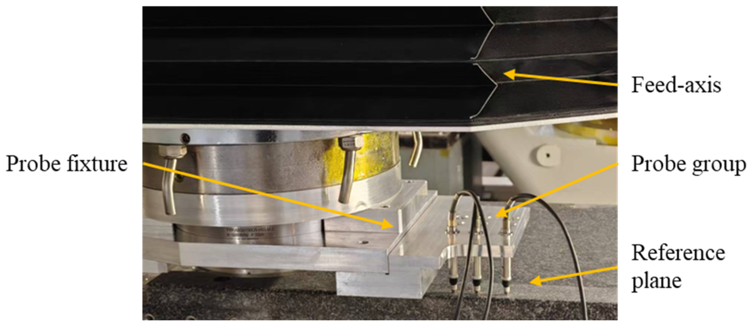
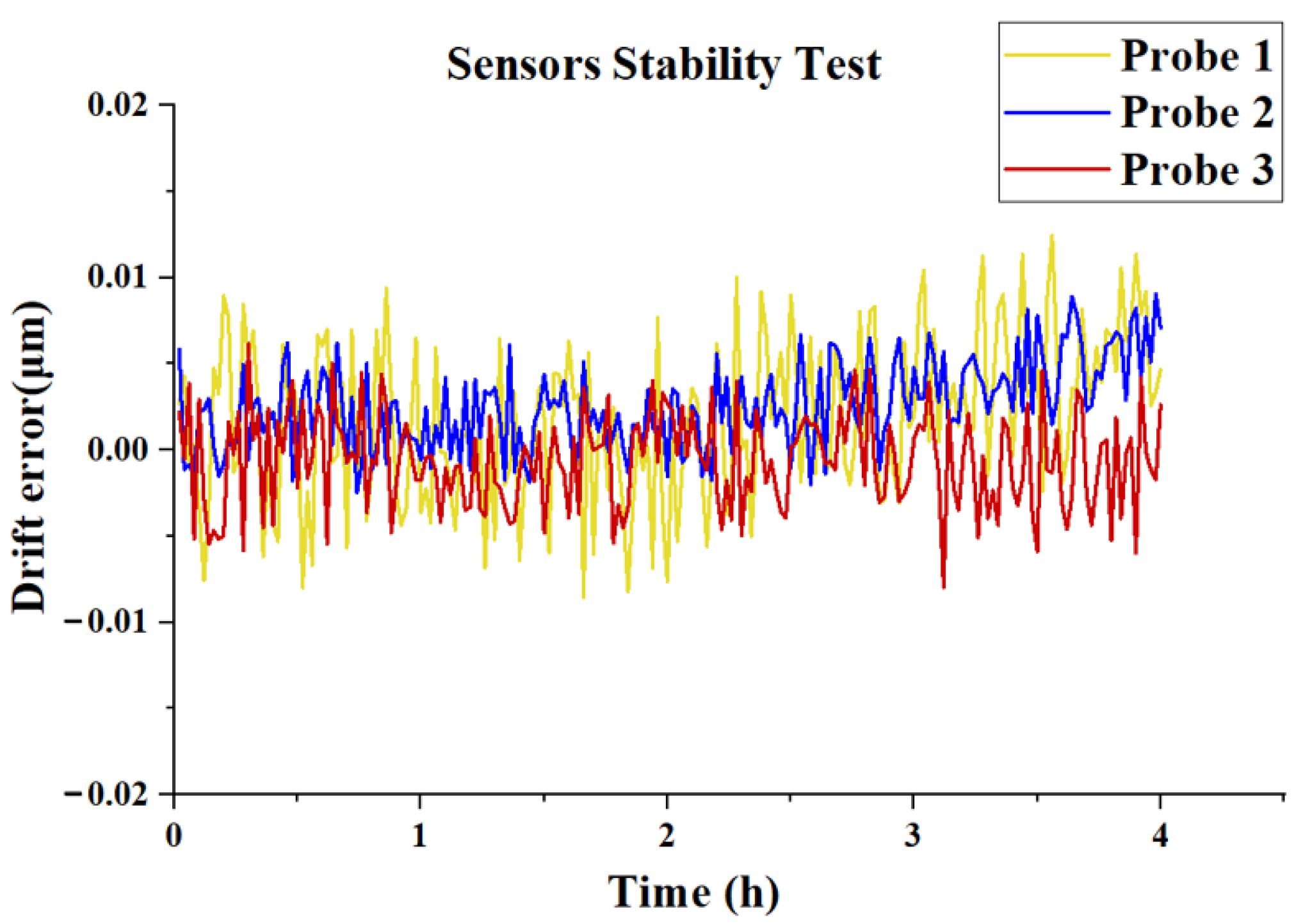
The sensor system employed a tri-probe configuration for data acquisition on a high precision Grade 000 granite reference plane (flatness tolerance ≤0.15 μm over 1000 mm2). To mitigate external dynamic disturbances, both the probe assembly and workpiece were mounted on a vibration-damped mounting platform with active isolation mechanisms, as shown in Figure 10.
Results indicate the sensor maintained a peak-to-peak noise level of ±12 nm over 30 min (Figure 11). Short-term noise, measured over 60 s intervals, remained consistently below ±10 nm. These outcomes validate the probe’s compliance with ISO 230-2 standards [24] for ultra-precision metrology equipment, confirming its suitability for sub-micron surface topography scanning applications.

3.4. Experiment System Measurement Uncertainty Tests

This experiment aims to rigorously evaluate the stability and repeatability of a flatness measurement system by comparing its results against the certified flatness of a Grade 000 marble reference plate (1000 mm × 500 mm). The plate’s permissible flatness deviation is ≤2.5 μm.
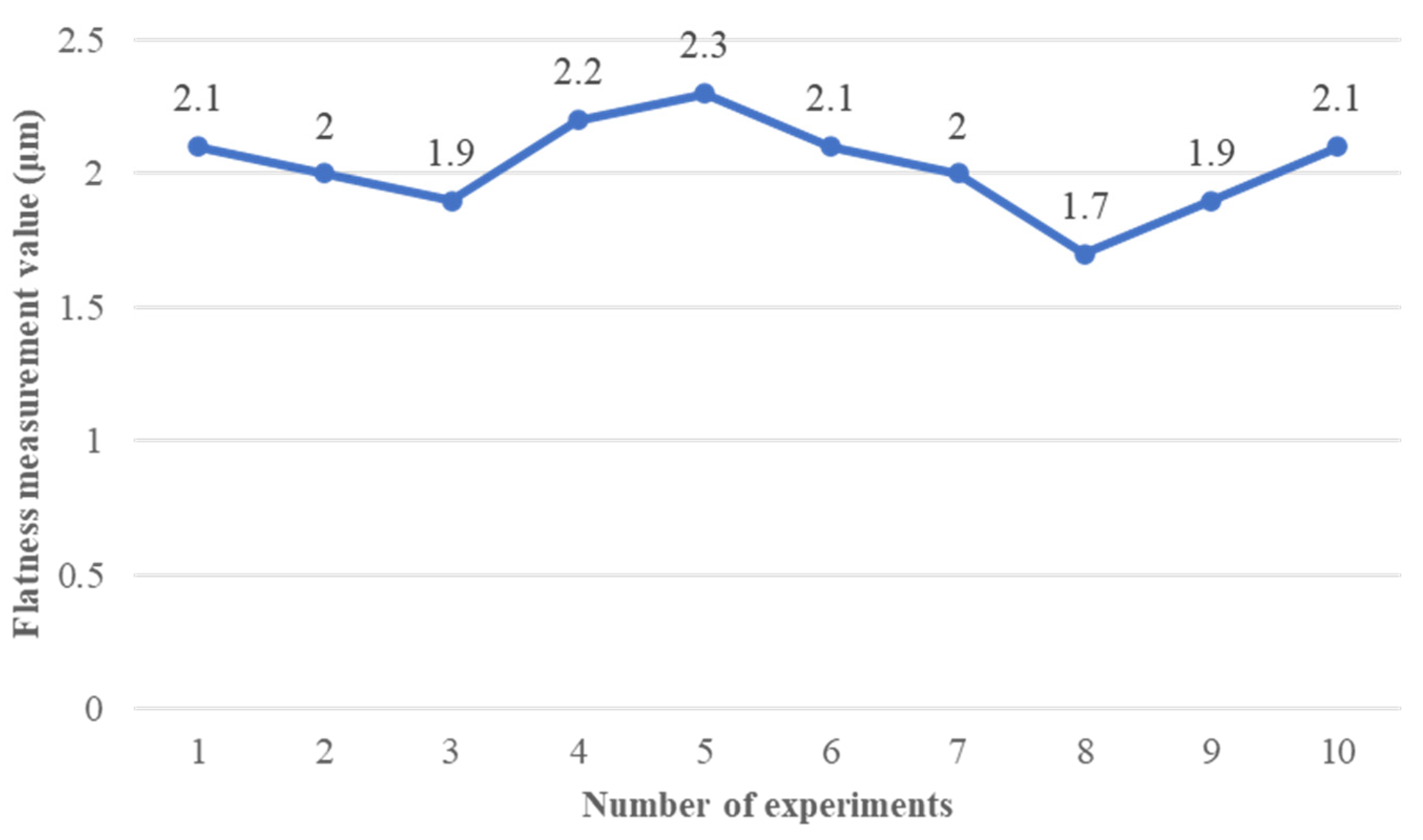
The Grade 000 marble reference plate (1000 mm × 500 mm, GB/T 20428-2006 [25], permissible flatness ≤ 2.5 μm) was verified via 10 repeated scans: (1) all measured flatness values (1.7–2.3 μm) fell within the permissible tolerance; (2) the mean measured value (2.0 μm) matched the plate’s certified flatness, confirming system accuracy.
A 100 × 50 grid of measurement points spaced at 10 mm intervals was defined across the plate surface. Figure 12 illustrates the probe spacing ( l 1 = 20   m m , l 2 = 30   m m ,   Δ l = 10   m m ) and sampling grid distribution, ensuring compliance with the probe position requirement ( l 1 =   Δ l × k , Section 2.1) and full coverage of the reference plate. Each point was sampled three times per full-grid scan, with the mean value recorded. Ten consecutive scans were performed to assess equipment performance.
As shown in Figure 13, the ten scans yielded flatness values ranging from 1.7 μm to 2.3 μm (mean 2.0 μm, range 0.6 μm, repeatability standard deviation 0.32 μm), demonstrating excellent short-term stability. Single-point triplicate measurements exhibited a maximum deviation of 0.2 μm, outperforming the equipment’s nominal repeatability specification of 0.5 μm.
Flatness was calculated via the least-squares method (in accordance with GB/T 11337-2004 [26], equivalent to ISO 12781-2:2011 [27]). The calculation process: fit an ideal plane by least-squares, compute each actual surface point’s deviation from this plane, and take the sum of absolute values of maximum positive and negative deviations as flatness error. The calculated flatness showed a peak-to-valley deviation of 1.1 μm (+0.7 μm maximum positive deviation, −0.4 μm maximum negative deviation). Statistical analysis of the ten scans revealed a mean flatness of 2.0 μm (max 2.3 μm, min 1.7 μm). All measurements fell within the Grade 000 tolerance band (≤2.5 μm), confirming high conformity between the system’s results and the reference standard.

4. Experimental Verification of Measurement System Performance

4.1. Experiment Design

To quantify the performance advantages of the nine-probe system, a comparative evaluation was conducted against the Dantsin Wyler BlueLEVEL electronic level (Switzerland; resolution 0.001 mm/m, range ±20 mm/m). The experiment was performed on a standard workpiece (nominal flatness 20 μm) under thermostatic control at 20 ± 0.5 °C, employing two measurement protocols:
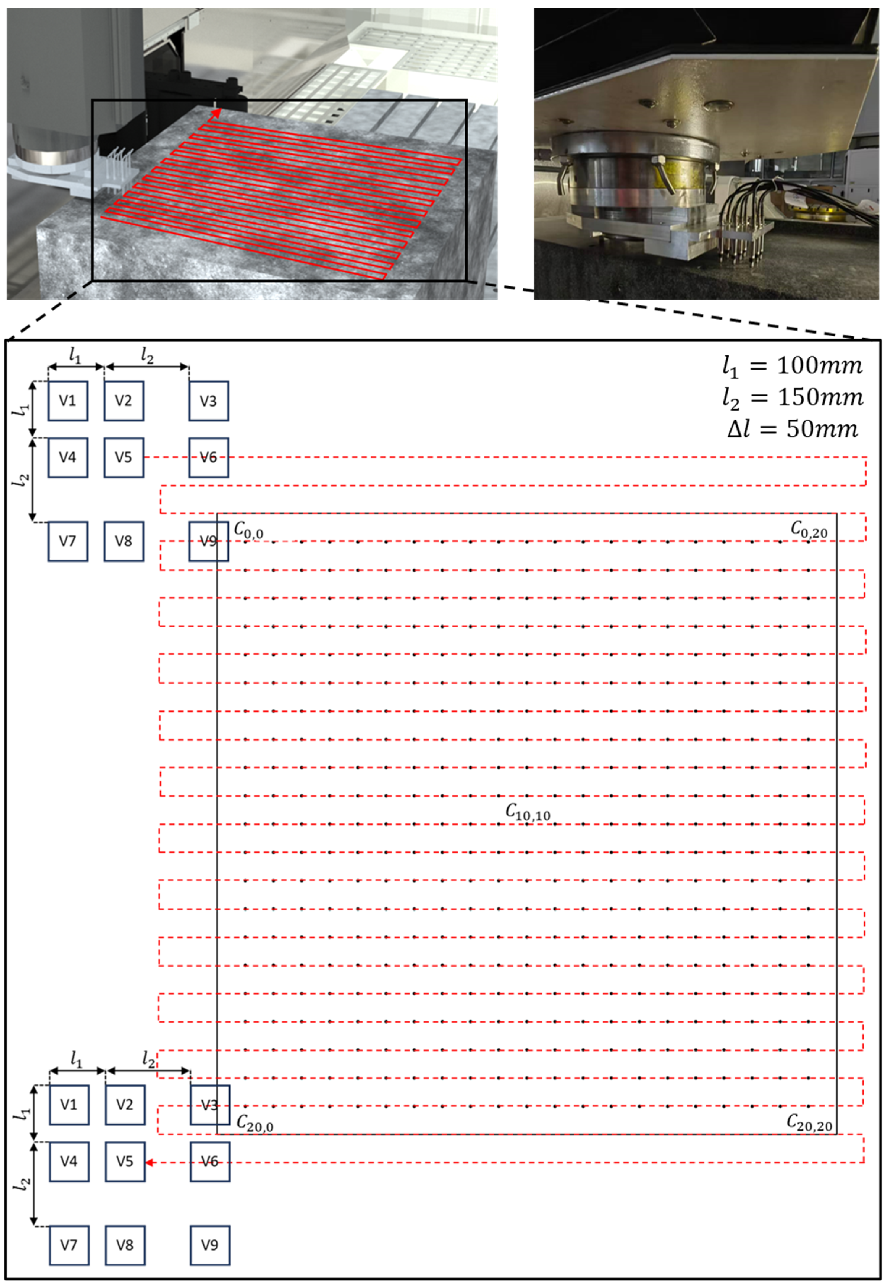
Nine-probe system: The system automatically executes a grid scan over a 1000 mm × 1000 mm area with 50 mm point spacing, acquiring 441-point data (21 × 21 grid). Z-direction elevations are logged in Excel, and flatness error is computed via the least-squares method. Probe traversal follows the programmed path depicted in Figure 14.
Manual electronic level measurement: This method utilizes a 100 mm grid spacing for point placement, with height differences measured using a bridge plate and electronic level. Figure 15 shows the electronic level measurement setup (bridge plate + level) and 100 mm grid layout, where sequential height difference accumulation from the datum point ( C 0,0 ) ensures consistent reference for all points. Post-measurement, the accumulation method is applied to reference all points to a common baseline, aligning measurements through sequential height difference accumulation from the initial datum point. Post-measurement, the accumulation method is applied to reference all points to a common baseline, aligning measurements through sequential height difference accumulation from the initial datum point.

4.2. Experiment Results

4.2.1. Nine Probe Method Measurement Results

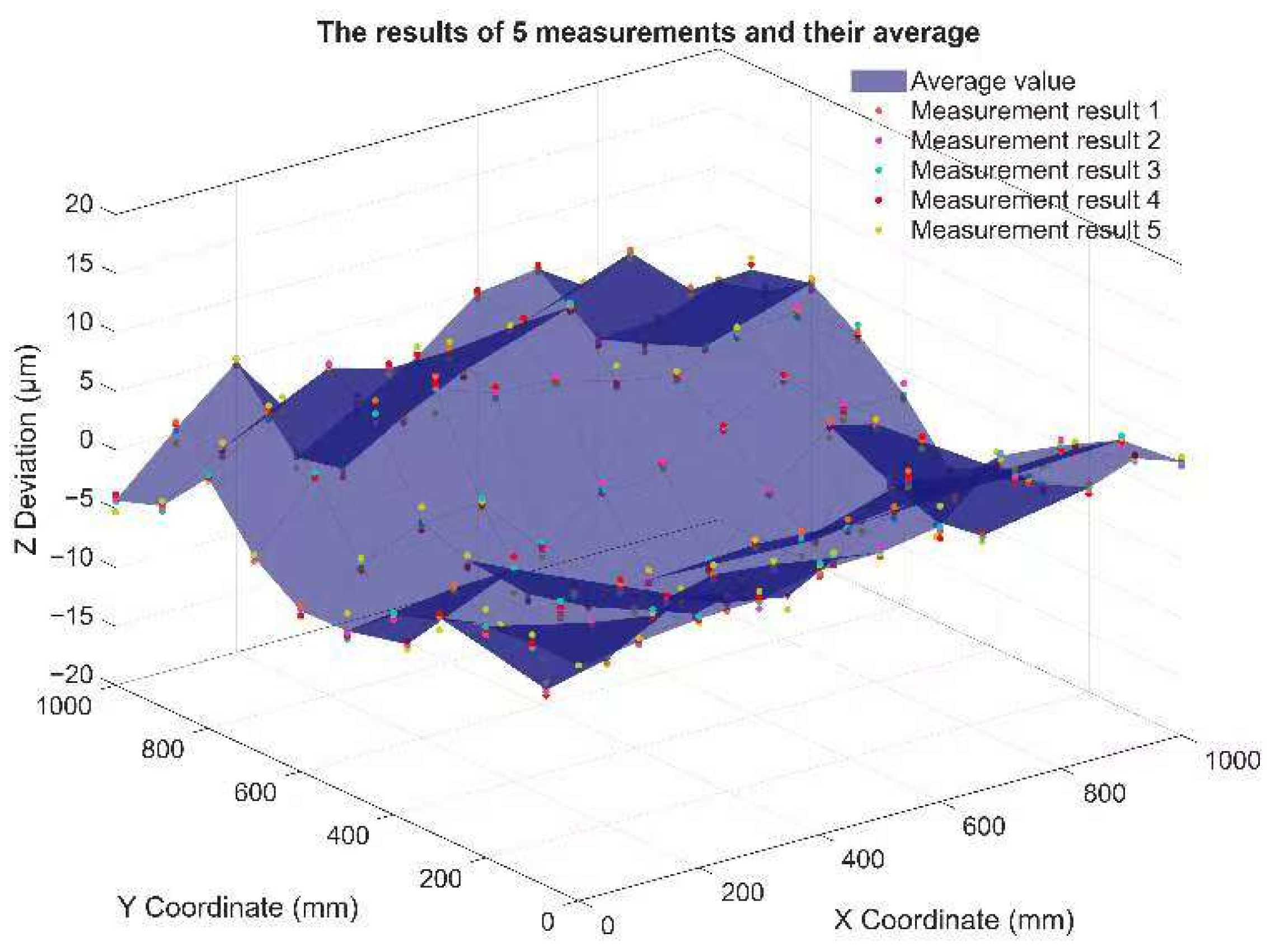
Figure 16 depicts the mean Z-direction elevation profiles from five repeated measurements. Comprehensive statistical analysis yields an average flatness error of 19.55 μm (calculated via the minimum zone method, Clause 5.2.2 of GB/T 11337-2004 [26]) with a standard deviation (σ, n = 5) of 0.627 μm for the flatness errors. The mean measurement duration per trial is 28.2 min.
For repeatability evaluation (Clause 6.3 of GB/T 11337-2004 [26]), the deviation of each individual measurement relative to the 5-measurement mean (19.55 μm) ranges from −10 nm to +25 nm. This slight asymmetric dispersion is attributed to minor local topographic variations of the workpiece surface, and the overall standard deviation of these relative deviations (0.11 μm, 110 nm) still meets the system’s repeatability requirement (≤0.32 μm, Section 3.4).

4.2.2. Electronic Level Method Measurement Results

Figure 17 illustrates the average Z-direction elevations across five measurement cycles. Statistical analysis reveals an average flatness error of 19.30 μm (calculated via the minimum zone method, Clause 5.2.2 of GB/T 11337-2004 [26]) with a standard deviation (σ, n = 5) of 0.684 μm for the flatness errors. The mean measurement time per trial is 62 min.
For repeatability evaluation (Clause 6.3 of GB/T 11337-2004 [26]), the deviation of each individual measurement relative to the 5-measurement mean (19.30 μm) falls within [−15 nm, +15 nm], with a corresponding standard deviation of 0.08 μm (80 nm). This result is consistent with the nominal repeatability of the Dantsin Wyler BlueLEVEL electronic level (0.1–0.2 μm for 1 m × 1 m flatness measurement), confirming data reliability.

4.2.3. Comparative Analysis of Measurement Outcomes

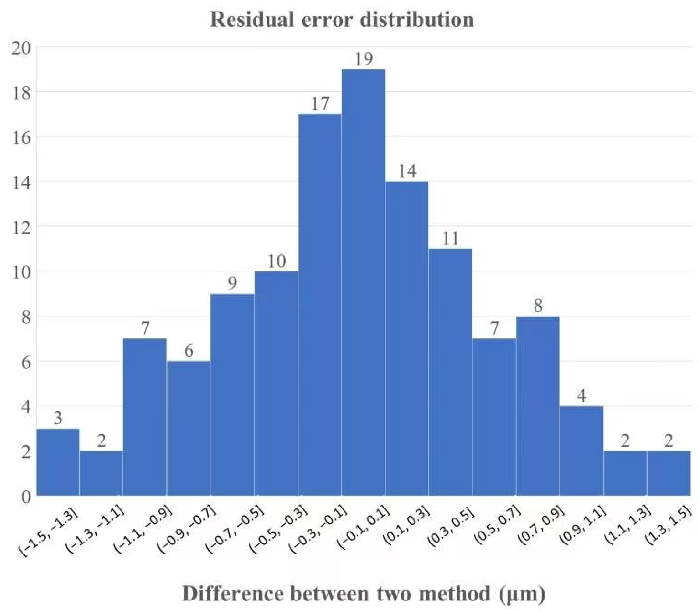
As shown in Figure 18, the residual error between the two methods is within [−1.5 μm, +1.5 μm]. Histogram analysis in Figure 19 confirms an approximately normal data distribution, the error statistics were listed in Table 1, where error magnitude correlates with occurrence frequency—indicating high consistency between measurement approaches. The nine-probe system demonstrates distinct industrial advantages:
Measurement Efficiency: 54.5% reduction in scan time (62 min → 28.2 min).
Spatial Resolution: The 441-point sampling grid (21 × 21) at 50 mm intervals exhibits a 4× higher spatial data density than the 121-point (11 × 11) grid used in the electronic level method (100 mm spacing). This denser sampling enables superior identification of localized form errors, while simultaneously balancing measurement throughput and geometric feature resolution.

5. Conclusions

This study addresses technical bottlenecks of traditional flatness measurement in ultra-precision machine tool manufacturing (low efficiency, poor repeatability, difficult error separation) and develops a high-precision integrated system. Core findings from theoretical modeling, system development, and experimental verification are summarized as follows:
Addresses three core limitations of traditional methods: Aiming at low manual sampling efficiency, environmental interference-induced repeatability errors, and difficult decoupling of machine tool motion errors from workpiece deviations, the system integrates FSTRP error separation and real-time adaptive sampling. This enables accurate decoupling of guideway motion errors (e.g., X/Y-axis straightness) and workpiece flatness deviations, avoiding “line-scan stitching” errors of traditional 1D multi-probe systems.
Innovates CNC-driven automated scanning: Unlike manual operation of traditional electronic levels, the system realizes automated scanning via machine tool CNC-nine-probe linkage. It eliminates external fixtures and manual alignment (cutting setup time by over 60% vs. traditional methods) and avoids human operation errors (e.g., inconsistent force application), ensuring data stability.
Enhances sampling density via 3 × 3 probe matrix: The 3 × 3 probe arrangement enables direct 2D full-field measurement. For a 1 m × 1 m area, it achieves 441 sampling points (21 × 21 grid, 50 mm interval)—4× that of traditional electronic levels (121 points, 11 × 11 grid, 100 mm interval), accurately identifying localized errors (e.g., micro-convexities) missed by low-density methods.
Ensures sub-micron repeatability with dual-error suppression: First, the FSTRP-based algorithm eliminates machine tool motion errors (compensated SD ≤ ±3 μm, meeting ISO 10360-5:2020 [28]). Second, adaptive sampling and high-precision capacitive probes (HD series: 1 nm resolution, ≤0.1% full-scale linear error) reduce environmental noise. Experiments show measurement repeatability SD 0.32 μm (Grade 000 granite plate), 30-min probe peak-to-peak noise ±12 nm.
Verifies accuracy and viability via experiments: Comparative tests with Dantsin Wyler BlueLEVEL (mainstream high-precision tool) show nine-probe system’s average flatness error 19.55 μm (minimum zone method, GB/T 11337-2004 [26]), highly consistent with electronic level’s 19.30 μm (residual errors −1.5~+1.5 μm); measurement time cut from 62 min to 28.2 min (54.5% efficiency gain). Five repetitions confirm flatness error SD 0.627 μm.
Provides metrology solution for measurement-machining integration: The system enables “on-machine measurement” (no workpiece disassembly), feeding results to CNC for real-time adjustment of large planar components (e.g., guideways, worktables). This closed-loop control improves ultra-precision machine tool manufacturing precision/efficiency, with value for high-end precision machinery batch production.
In conclusion, the proposed nine-probe system fills gaps in high-efficiency, high-density 2D flatness measurement for large precision components and provides a novel technical path for measurement-machining integration in ultra-precision manufacturing. Future research will optimize probe calibration and extend applicability to curved surface measurement.

Author Contributions

Writing—original draft preparation, H.L. and Y.H.; Research Design, H.L. and J.C.; data analysis, H.L. and H.Y.; data collection, Z.P. and X.L.; make charts, Z.P. and X.L.; literature search, H.Y. All authors have read and agreed to the published version of the manuscript.

Funding

This research was funded by [Wuhan Science and Technology Plan Project, Research and Application of New-generation Intelligent Numerical Control System and Typical Intelligent Technology] grant number [2023010402040013].

Data Availability Statement

The raw data supporting the conclusions of this article will be made available by the authors on request.

Conflicts of Interest

Author Hua Liu, Zexin Peng and Xinyu Liu were employed by the company Jiangxi JUST Machine Tool Co., Ltd. The remaining authors declare that the research was conducted in the absence of any commercial or financial relationships that could be construed as a potential conflict of interest.

References

  1. Dichev, D.; Diakov, D.; Zhelezarov, Y.; Nikolova, H.; Kupriyanov, O.; Dicheva, R. Accuracy Evaluation of Flat Surfaces Measurements in Conditions of External Influences. Machines 2021, 9, 156. [Google Scholar] [CrossRef]
  2. Huang, S.; Pang, Y.; Xia, H. Data Preprocessing for Flatness Measurements of Large Precision Workpieces. J. Phys. Conf. Ser. 2024, 2770, 012014. [Google Scholar] [CrossRef]
  3. Shu, H.; Zou, C.; Chen, J.; Wang, S. Research on Micro/Nano Surface Flatness Evaluation Method Based on Improved Particle Swarm Optimization Algorithm. Front. Bioeng. Biotechnol. 2021, 9, 775455. [Google Scholar] [CrossRef]
  4. Saleh, A.A.; Amer, M.; Nada, N. Investigation of Error Sources in Absolute Flatness Measurement Using Fizeau Interferometer. Opt. Eng. 2024, 63, 101502. [Google Scholar] [CrossRef]
  5. Liu, Y.; Yu, C.; Liang, X.; Qiu, Z.; Zhang, X.; Lian, C.; Li, J.; Ji, J.; Shan, P.; Lyu, X.; et al. Genetic Algorithms and Machine Learning Enhanced Laser Displacement Sensor Point Cloud Augmentation for Low-Cost, Large-Scale Flatness Measurements. IEEE Sens. J. 2023, 23, 22189. [Google Scholar] [CrossRef]
  6. Zhou, L.; Zheng, N.; Li, J.; Yuan, Z.; Wang, J.; Fang, F.; Xu, Q. Splicing Measurement and Compensation of Straightness Errors for Ultra-Precision Guideways. Micromachines 2023, 14, 1670. [Google Scholar] [CrossRef]
  7. Miko, B. Assessment of Flatness Error by Regression Analysis. Measurement 2022, 188, 110542. [Google Scholar] [CrossRef]
  8. Yang, D.; Zou, J. Precision Analysis of Flatness Measurement Using Laser Tracker. Sensors 2023, 23, 7890. [Google Scholar] [CrossRef]
  9. Dichev, D.; Diakov, D.; Zhelezarov, I.; Valkov, S.; Ormanova, M.; Dicheva, R.; Kupriyanov, O. A Method for Correction of Dynamic Errors When Measuring Flat Surfaces. Sensors 2024, 24, 5154. [Google Scholar] [CrossRef]
  10. Mathews, R.; No, T.; Honeycutt, A.; Tyler, C.; Smith, S. Rapid Commissioning of Large Machine Tools Using Finite Element-Based Correction of Geometric Errors. Precis. Eng. 2024, 78, 101–112. [Google Scholar] [CrossRef]
  11. Su, H.; Ye, R.; Cheng, F.; Cui, C.; Yu, Q. A Straightness Error Compensation System for Topography Measurement Based on Thin Film Interferometry. Photonics 2021, 8, 149. [Google Scholar] [CrossRef]
  12. Lai, T.; Liu, J.; Chen, F.; Li, Z.; Guan, C.; Xu, C.; Hu, H.; Dai, Y.; Chen, S.; Dai, Z. Allocation of Geometrical Errors for Developing Precision Measurement Machine. J. Manuf. Mater. Process. 2024, 8, 124. [Google Scholar] [CrossRef]
  13. Kiyono, S.; Gao, W. Profile Measurement of Machined Surface with a New Differential Method. Precis. Eng. 1994, 16, 212–218. [Google Scholar] [CrossRef]
  14. Chai, N.; Yin, Z.; Yao, J. High Accuracy Profile Measurement with a New Virtual Multi-Probe Scanning System. IEEE Access 2020, 8, 158727–158734. [Google Scholar] [CrossRef]
  15. Gao, W.; Yokoyama, J.; Kojima, H.; Kim, S.-W. Precision Measurement of Cylinder Straightness Using a Scanning Multi-Probe System. Int. J. Mach. Tools Manuf. 2007, 47, 1053–1058. [Google Scholar] [CrossRef]
  16. Li, F.; Li, H.; Kim, M.-K.; Lo, K.-C. Laser Scanning Based Surface Flatness Measurement Using Flat Mirrors for Enhancing Scan Coverage Range. Remote Sens. 2021, 13, 714. [Google Scholar] [CrossRef]
  17. Xiao, S.; Wu, J.; Lai, N.; Lin, R.; Qiao, M.; Wang, Z.; Luo, W.; Fu, Y.; Liang, P.; Zhou, P.; et al. Research on Flatness Measurement of Large-Size Parts Based on 3-D Machine Vision. IEEE Trans. Instrum. Meas. 2023, 72, 3514812. [Google Scholar] [CrossRef]
  18. Elmelegy, A.; Zahwi, S. Comparative Study of Error Determination of Machine Tools. Int. J. Adv. Manuf. Technol. 2023, 127, 4329–4341. [Google Scholar] [CrossRef]
  19. Hwang, J.; Park, C.-H.; Gao, W.; Kim, S.-W. A Three-Probe System for Measuring the Parallelism and Straightness of a Pair of Rails for Ultra-Precision Guideways. Int. J. Mach. Tools Manuf. 2007, 47, 1053–1058. [Google Scholar] [CrossRef]
  20. Stauffenberg, J.; Ortlepp, I.; Belkner, J.; Dontsov, D.; Langlotz, E.; Hesse, S.; Rangelow, I.; Manske, E. Measurement Precision of a Planar Nanopositioning Machine with a Range of Motion of Ø100 mm. Appl. Sci. 2022, 12, 7843. [Google Scholar] [CrossRef]
  21. Yang, P.; Takamura, T.; Takahashi, S.; Takamasu, K.; Sato, O.; Osawa, S.; Takatsuji, T. Development of high-precision micro-coordinate measuring machine: Multi-probe measurement system for measuring yaw and straightness motion error of XY linear stage. Precis. Eng. 2011, 35, 424–430. [Google Scholar] [CrossRef]
  22. Manske, E.; Fröhlich, T.; Füßl, R.; Ortlepp, I.; Mastylo, R.; Blumröder, U.; Dontsov, D.; Kühnel, M.; Köchert, P. Progress of nanopositioning and nanomeasuring machines for cross-scale measurement with subnanometre precision. Meas. Sci. Technol. 2020, 31, 085005. [Google Scholar] [CrossRef]
  23. ISO 230-1:2012; Test Code for Machine Tools—Part 1: Geometric Accuracy of Machines Operating Under no-Load or Quasi-Static Conditions. ISO: Geneva, Switzerland, 2012.
  24. ISO 230-2:2014; Test Code for Machine Tools—Part 2: Determination of Accuracy and Repeatability of Positioning of Numerically Controlled Axes. ISO: Geneva, Switzerland, 2014.
  25. GB/T 20428-2006; Granite Surface Plates. China Machinery Industry Federation: Beijing, China, 2006. Available online: https://openstd.samr.gov.cn/bzgk/gb/newGbInfo?hcno=371394233DD71C7948B402F26D38D001 (accessed on 7 September 2025).
  26. GB/T 11337-2004; Measurement of Departures from Flatness. China Machinery Industry Federation: Beijing, China, 2004. Available online: https://openstd.samr.gov.cn/bzgk/gb/newGbInfo?hcno=3EB9458F0BBAC9DE0C78CD60776E1D3F (accessed on 7 September 2025).
  27. ISO 12781-2:2011; Geometrical Product Specifications (GPS)—Flatness, Part 2: Specification Operators. ISO: Geneva, Switzerland, 2011. Available online: https://www.iso.org/standard/53625.html (accessed on 7 September 2025).
  28. ISO 10360-5:2020; Geometrical Product Specifications (GPS)—Acceptance and Reverification Tests for Coordinate Measuring Systems (CMS), Part 5: Coordinate Measuring Machines (CMMs) Using Single and Multiple Stylus Contacting Probing Systems Using Discrete Point and/or Scanning Measuring Mode. ISO: Geneva, Switzerland, 2010. Available online: https://www.iso.org/standard/73431.html (accessed on 7 September 2025).
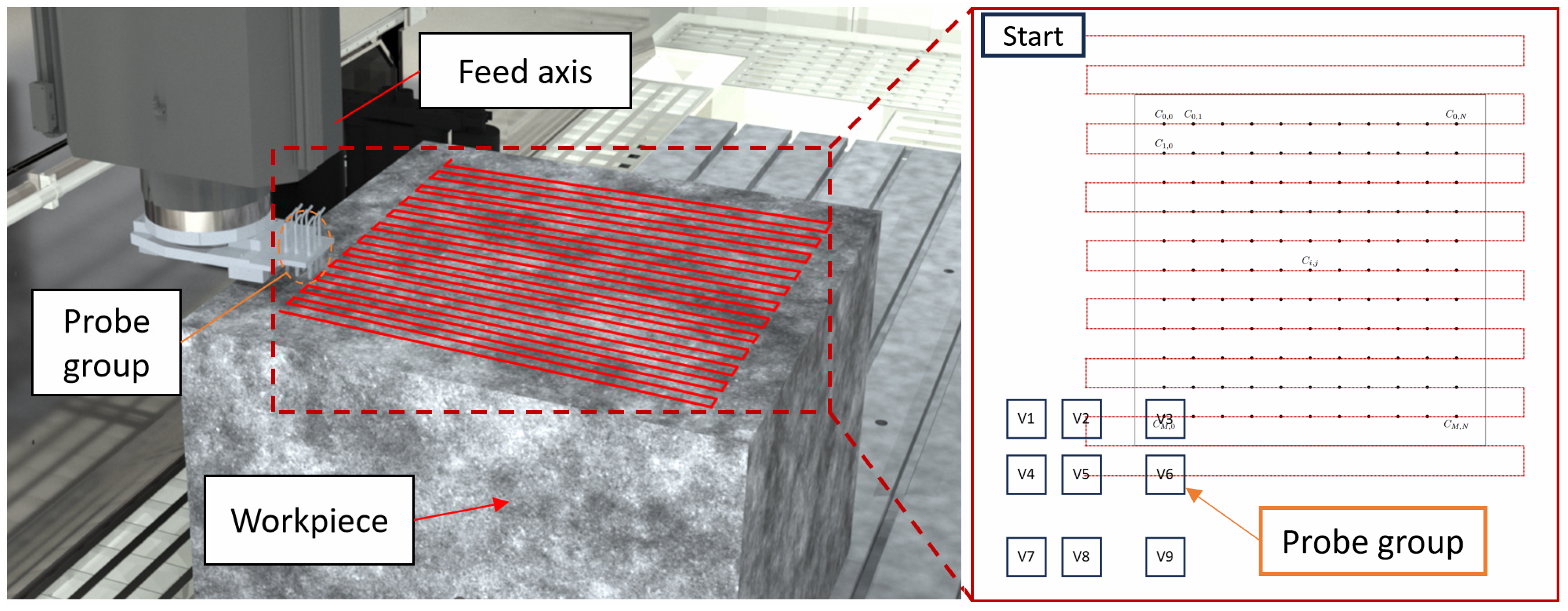
Figure 1. Measurement Principle and Prototype.
Machines 13 00856 g001
Figure 2. Probe group with structural details.
Machines 13 00856 g002
Figure 3. Working principle of measurement system.
Machines 13 00856 g003
Figure 4. Error separation principle for the X-direction probe group (general).
Machines 13 00856 g004
Figure 5. Six steps to separate the error by X-direction probe group.
Machines 13 00856 g005
Figure 6. Experimental measurement system.
Machines 13 00856 g006
Figure 7. Schematic diagram of uncertainty testing.
Machines 13 00856 g007
Figure 8. Photo of machine tool accuracy and repeatability tests (a) Measurement in X-axis; (b) Measurement in Y-axis; (c) Measurement in Z-axis. 1. Feed axis 2. Target Reflector 3. Laser Tracker Head.
Machines 13 00856 g008
Figure 9. Machine tool accuracy measurement result. (a) X-axis position error. (b) X-axis horizontal straightness. (c) X-axis vertical straightness. (d) Y-axis position error. (e) Y-axis horizontal straightness. (f) Z-axis vertical straightness. (g) Z-axis position error. (h) Z-axis horizontal straightness. (i) Z-axis vertical straightness.
Machines 13 00856 g009
Figure 10. Sensors stability test.
Machines 13 00856 g010
Figure 11. Measurement stability data of the employed probe.
Machines 13 00856 g011
Figure 12. Schematic diagram of measurement process.
Machines 13 00856 g012
Figure 13. Flatness measurement repeatability.
Machines 13 00856 g013
Figure 14. Schematic diagram of nine-probe measurement system and prototype photograph.
Machines 13 00856 g014
Figure 15. Schematic diagram of electronic level measurement system and photograph.
Machines 13 00856 g015
Figure 16. Measurement result from the nine-probe method.
Machines 13 00856 g016
Figure 17. Measurement result from electronic level method.
Machines 13 00856 g017
Figure 18. Residual error between two methods.
Machines 13 00856 g018
Figure 19. Residual error distribution.
Machines 13 00856 g019
Table 1. Error Statistics Table.
Maximum Positive ErrorMaximum Negative ErrorAverage ErrorStandard DeviationP-V Error
1.39 µm−1.44 µm−0.07537 µm0.71702.83 µm
Disclaimer/Publisher’s Note: The statements, opinions and data contained in all publications are solely those of the individual author(s) and contributor(s) and not of MDPI and/or the editor(s). MDPI and/or the editor(s) disclaim responsibility for any injury to people or property resulting from any ideas, methods, instructions or products referred to in the content.