Abstract
The variable camber morphing wing has the potential to achieve improved flight performance across different flight conditions by changing its geometry according to changing flight conditions. Evaluating the subtle aerodynamic benefits of variable camber technology necessitates wind tunnel testing under flight Reynolds number conditions. In high Reynolds number wind tunnels, the cryogenic environment readily damages model surface profiles through desublimation and frost, compromising test data accuracy. Consequently, cryogenic wind tunnels must enforce rigorous water vapor control standards. To address potential water vapor effects during cryogenic wind tunnel testing, high-resolution optical measurement techniques were employed to quantify the spatiotemporal evolution of desublimation frost thickness on a typical supercritical airfoil surface. Combined with numerical simulations, the mechanisms governing the frost layer’s influence on aerodynamic characteristics and flow field structures were systematically investigated. The results reveal that the influence of water vapor desublimation on the aerodynamic characteristics under diverse cryogenic working conditions has a commonality, and the difference in aerodynamic parameters shows an increasing tendency as the frost time increases; water vapor desublimation has an obvious influence on the flow structure of the airfoil and its pressure distribution on the surface, which increases flow instability and leads to the backward shift of the shock wave position; larger frost thickness gradients along the flow direction cause more drastic changes in pressure distribution and flow structure; and a larger rate of water vapor desublimation results from a lower temperature and a higher concentration of water vapor in the test environment, which causes frosting to have a more severe impact on the airfoil’s aerodynamic characteristics and flow structure. The findings establish a technical basis for cryogenic wind tunnel moisture control standards and provide a solid foundation for the refined assessment of aerodynamic benefits of the camber morphing wing.
1. Introduction
Aircraft must maintain exceptional aerodynamic characteristics in addition to adapting to a variety of flight environments due to the growing need for cross-domain flight and multi-mission execution [1]. However, conventional rigid airfoils typically represent a compromise across multiple flight regimes, demonstrating good aerodynamic characteristics only near the design point while exhibiting significant limitations in off-design flight conditions [2]. The rapid development of smart flexible materials has positioned morphing wings as a growing research focus in next-generation intelligent aircraft design. By real-time reconfiguration of their geometry, these wings adaptively alter their aerodynamic profiles to achieve global performance optimization, representing a critical pathway to overcome fixed-configuration design constraints [3]. Shape-adaptive technologies, represented by flexible trailing edge variable-camber techniques, have been progressively implemented in aviation with substantial application prospects [4,5,6,7]. Large transport aircraft and other advanced aviation vehicles typically feature substantial dimensions and high flight Reynolds numbers. During transonic flight, viscous flow structures governed by Reynolds number emerge on wing surfaces, including boundary layer development, laminar-to-turbulent transition, and shock wave-boundary layer interactions [8]. These flow structures significantly influence vehicle aerodynamic performance parameters, thereby complicating the assessment of aerodynamic gains from shape-adaptive technologies [9].
The most reliable way to obtain aerodynamic information about a vehicle is through a wind tunnel test. Throughout the wind tunnel test, some similarity criteria must be met. The Reynolds number is one of the most crucial of these factors [10]. The Reynolds number, which describes the proportion of fluid inertial and viscous forces, is an important parameter for flow type and evolution. The Reynolds number has a significant effect on the viscous and differential pressure drag of the vehicle, which can be determined by changing the flow stability of the boundary layer to determine whether it is a laminar or turbulent boundary layer, which directly affects the drag characteristics of the vehicle. On the other hand, the Reynolds number also determines the structure and scale of the small-scale vortices in the boundary layer, which play a key role in dissipating the energy generated by the large-scale vortices to maintain the dynamic equilibrium of the system, and the complex coupling relationship with the large-scale vortex structure inevitably influences the external large-separated flow field, which has an impact on the surface pressure distribution, lift and drag characteristics, and pitching moment [11]. The transition characteristics between the large-scale vortex structures in the external flow field and the small-scale vortex structures within the boundary layer become more complex as the Reynolds number rises, making it more challenging to determine the vehicle’s aerodynamic characteristics [12]. Additionally, the transonic wind tunnel test Reynolds number for large aircraft is typically an order of magnitude lower than the flight Reynolds number. This causes the simulation of the flow structure to be distorted, including the separation of the boundary layer and transition, and makes it challenging to precisely determine their aerodynamic characteristics. One of the main technologies impeding the development of sophisticated vehicles is the standard transonic wind tunnels’ inadequate capacity to simulate Reynolds numbers [13].
The optimum method to raise the Reynolds number in wind tunnel testing, according to theory and practice, is to reduce the overall temperature of the incoming flow [14,15,16,17,18]. This method utilizes nitrogen as the working medium, significantly enhancing the test Reynolds number by reducing the total gas temperature, decreasing gas viscosity, increasing density, and combining with appropriate pressurization [19]. Since the 1970s, more than 20 cryogenic wind tunnels have been successfully constructed internationally. The United States and Europe have built large-scale production cryogenic wind tunnels (NTF, ETW), achieving the ground simulation of the Reynolds number for large aircraft flight [20,21,22,23,24]. In contrast to traditional wind tunnels, cryogenic wind tunnels function at low temperatures (110 K) and have a wide temperature range (110 K to normal temperature). As a result, all test components must have extremely high dew point requirements to prevent trace water desublimation from compromising the model’s surface shape and lowering the quality of the wind tunnel test data [25]. Water contamination is an inevitable problem in cryogenic wind tunnel operation, as demonstrated by NTF and ETW’s operational experience. For this reason, many wind tunnels have unique drying conditions (such as drying halls) to keep the models dry throughout condition changes and transfers. However, the operation of a drying hall necessitates a balance between water vapor content, operating expenses, and data quality. This entails complicated difficulties, including determining the impact of trace water desublimation and its degree, which can be challenging. Thus, exploring the influence of laws of frost formation on model surfaces upon the flow structures and aerodynamic characteristics of aircraft under cryogenic conditions can effectively support quantitative assessment of water vapor content in cryogenic wind tunnel drying chambers, thereby ensuring data quality in wind tunnel tests at flight Reynolds numbers for variable-camber wings.
Therefore, to accurately capture the aerodynamic performance improvement effect brought by the wing variable-camber technology, it is necessary to conduct targeted tests in cryogenic wind tunnels. However, due to the cryogenic characteristics of cryogenic wind tunnels, during the transfer of the test model to the drying hall, the model surface is prone to frost formation caused by the desublimation of ambient water vapor when it encounters cryogenic temperatures. This phenomenon not only directly alters the original geometric shape of the wing but may also interfere with the actual trailing edge camber of the wing after active variable-camber adjustment, which ultimately makes it difficult for the variable-camber wing wind tunnel test to accurately simulate its real aerodynamic performance, thereby affecting the precise evaluation of the aerodynamic gains of the variable-camber technology. Based on this, it is an urgent need to carry out a dedicated study on the influence of water vapor desublimation and frost formation on the wing surface on its aerodynamic performance.
In this paper, a numerical and experimental study are performed together to investigate the effect on the variable camber wing, which is affected by the water vapor desublimation. At first, the model definition is given in Section 2, and the corresponding numerical simulation method is explained, which is validated by a case study. Then, in Section 3, experimental study is undertaken to measure the real-world airfoil geometry change due to the water vapor desublimation effect, which lays down the foundation for the numerical study. At last, the effect of the water vapor desublimation on the aerodynamic characteristics of the airfoil is investigated, with the geometry change obtained in Section 3.
2. Model Definition and the Numerical Simulation Method
2.1. Model Definition
2.1.1. Cryogenic Wind Tunnel Drying Hall
The drying hall is an important part of the model transfer system, mainly used to keep the surface of the model in a dry state during the process of entering and exiting the test section before and after the condition change, which usually requires that the water vapor and carbon dioxide content in the drying hall is low enough and the surface of the model is free of frost. However, there are certain unique features of the drying hall of a large cryogenic wind tunnel, such as its huge volume, low dew point, challenging airflow organization, etc. [26]. Its low dew point level is hard to maintain, and there is always some water vapor in the hall, which makes it easy for frost to form on the model’s surface. This has a significant impact on the flow field’s characteristics on the model’s surface as well as the quality of test data. Given that drying halls are the primary risk for water vapor contamination, appropriate studies were conducted for this environment.
2.1.2. Supercritical Airfoil
To accurately quantify the aerodynamic gains of wing camber morphing technology, this study focuses on the practical engineering application issues of camber morphing technology and conducts an analysis by integrating the model storage and transfer scenarios in the cryogenic wind tunnel drying hall. When the temperature and humidity of the camber-morphing wing model are regulated in the drying hall, residual water vapor in the environment can desublimate into frost on the wing surface (Figure 1). The adhesion of the frost layer induces two-fold effects: first, it causes an unanticipated alteration in the geometric profile of the camber-morphing wing, increasing the actual camber output error of the active camber-morphing control system; second, it disrupts the transonic flow structures, leading to significant distortion of flow field characteristics.
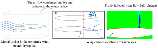
Figure 1.
Schematic of the water vapor desublimation on the camber morphing wing.
Given that the cruise speed of large aircraft mostly falls within the transonic range, their wings generally employ supercritical airfoils to optimize cruise efficiency. During transonic flight, the complex flows (including boundary layer development, shock waves, and their induced boundary layer separation) over the surface of a supercritical airfoil are extremely sensitive to the Reynolds number, which directly determines the accuracy of ground-test predictions for the aircraft’s aerodynamic characteristics such as drag, aerodynamic center, and maximum lift. Therefore, this study selects the classic RAE2822 supercritical airfoil. This airfoil features abundant test condition data and comparative information, providing reliable data support. By quantifying the interference law of frost on the aerodynamic characteristics (e.g., drag coefficient, lift-to-drag ratio) of camber-morphing wings, it supplies key data for the reliability verification of camber morphing technology in the transonic flight phase and the development of error compensation strategies.
2.2. Numerical Simulation Method
Using Reynolds Averaged Navier–Stokes (RANS) as the numerical solution method, numerical simulations are performed for the 2D RAE2822 baseline airfoil and frosted airfoil. The turbulence model is chosen from the two-equation SST K-Omega turbulence model and the Spalart–Allmaras (S-A) turbulence model, which is widely used in the aerospace industry.
2.2.1. Governing Equations
The motion of fluids adheres to Newton’s laws of motion, governed by three fundamental equations: the continuity equation, momentum equation, and energy equation. The governing equations for unsteady compressible fluid flow in a three-dimensional Cartesian coordinate system are described by the Navier–Stokes equations:
Continuity equation:
Momentum equation:
Energy equation:
where denotes the density of the fluid; denotes the pressure of the fluid; denotes the velocity component in the coordinate direction; denotes the total energy per unit mass of the fluid, that is, the sum of the internal and kinetic energies; denotes the fluid shear stress tensor; and denotes the heat flow power.
Where the following are the expressions for , , and :
where denotes the temperature of the fluid; denotes the specific heat ratio of the fluid, and the mass is air under this calculation condition, so is taken; denotes the viscosity coefficient; denotes the heat conduction coefficient.
Where Sutherland’s formula is used to determine the coefficient of viscosity, , as follows:
where, , in this calculation condition, the mass is air so take , .
The heat transfer coefficient, , is calculated as follows:
where refers to the Prandtl constant, which is typically assumed to be for air, and and refer to the specific heat at constant pressure and volume, respectively.
In order to close the aforementioned equations, the ideal gas equation of state must be added to the gas equation of state:
where is the gas constant of air, which takes the value .
2.2.2. Spalart–Allmaras Turbulence Model
The Reynolds stress term and the turbulent viscous coefficient must be found to solve the Reynolds Averaged Navier–Stokes equation. The Spalart–Allmaras turbulence model was developed by Spalart using a combination of quantitative and empirical studies; the model’s turbulent viscous coefficient can be expressed as follows:
The expression for the turbulent viscosity ratio is:
The transport equation for is:
The following is the interpretation of the coefficient values in the transport equation:
where is the closest distance between the object surface and a point in the flow field.
2.2.3. Computational Grid and Grid Independence Validation
The computational domain of the airfoil flow field is gridded using a C-shaped grid, a structured quadrilateral grid, in this study’s numerical simulation of 2D airfoils. To ensure grid independence and minimize computational cost, three grid configurations were implemented: coarse (74,000 cells), medium (105,000 cells), and fine (160,000 cells). The coarse grid exhibited near-wall Y+ values around 10, whereas both medium and fine grids maintained Y+ ≈ 1. Detailed grid parameters are documented in Table 1.

Table 1.
Grid Parameters.
Numerical simulations were conducted on RAE2822 baseline airfoil grids with three distinct grid configurations under incoming flow conditions of Ma = 0.729, angle of attack (α) 2.31°, and freestream temperature 255.56 K. The converged numerical results of lift coefficient (CD), drag coefficient (CD), and pitching moment coefficient (Cm, referenced about the airfoil leading edge) for the three grid configurations are tabulated in Table 2. By using the numerical simulation results of the dense grids as the reference, the relative errors of the findings for the sparse and medium grids are analyzed. The maximum relative error between medium and fine grid solutions is quantified at 0.14%, while the coarse grid exhibits a 3.79% maximum discrepancy specifically in drag coefficient prediction. With all three grid configurations demonstrating errors below the 4% threshold, these results confirm that grid resolution exerts minimal influence on the numerical simulation outcomes. Considering computational resource allocation, computational efficiency, and numerical accuracy, the medium grid was selected as the meshing strategy for this study.
Table 2.
Grid Independence Verification Results.
2.2.4. Validation of Computational Methods
The computational parameters selected in this study are based on the computational parameters set in the wind tunnel experiments, and the wind tunnel experimental data have been recorrected by combining the ideas proposed by Haass [27]. Using the airfoil chord length L = 0.3048 m for Reynolds number calculation, the finalized computational parameters are presented in Table 3.
Table 3.
Inflow Parameters.
The numerical simulations employed the finite volume method (FVM) to solve the 2D Navier–Stokes equations. A second-order upwind scheme was implemented for spatial discretization, coupled with an implicit solver. Steady-state simulations of the baseline RAE2822 airfoil were conducted using both the SST k-ω and Spalart–Allmaras turbulence models. To accurately represent real physical system boundaries during computational processes, appropriate boundary conditions must be defined throughout the simulation. For the computational domain, both initial and boundary conditions require systematic parametrization. Under transonic compressible viscous flow conditions, the following boundary conditions were established:
- (1)
- Far-Field Boundary Conditions
In regions distant from the wall surfaces within the flow field, the fluid velocity asymptotically approaches the freestream velocity. These zones were therefore idealized as freestream regions. Consequently, the freestream conditions were set as the far-field boundary conditions in the current computational framework, with specific parameterizations detailed below:
where denotes the freestream velocity, represents the angle of attack, and , indicate the velocity components along the x-direction and y-direction, respectively.
- (2)
- Wall Boundary Conditions
An adiabatic no-slip wall is selected for the object surface, under which the fluid velocity flowing through the wing wall is 0, .
Figure 2 compares the numerically predicted wall pressure coefficients using different turbulence models with experimental data [28] (denoted as Exp). The analysis demonstrates good agreement between the wall pressure coefficients predicted by different turbulence models and experimental data. This consistency validates both the feasibility of the computational methodology and the reliability of the numerical results. Specifically, the Spalart–Allmaras turbulence model achieves higher consistency with experimental values at the shock location compared to the SST k-ω model. Based on this comparative performance, the Spalart–Allmaras model is adopted for subsequent simulations.
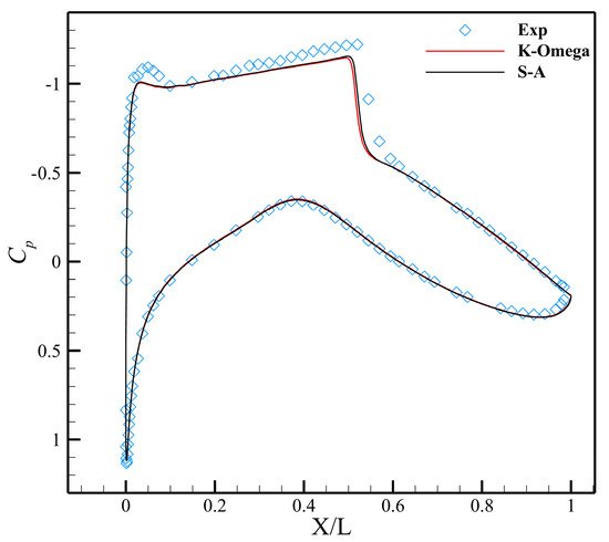
Figure 2.
Comparison of Wall Pressure Coefficients.
3. Effect of the Water Vapor De-Sublimation on the Airfoil Shape
3.1. Measuring Method
3.1.1. Ultra-Low Dew Point Test Environment Creation and Desublimation Test
Using the “replacement-purification and air distribution method,” a test chamber (Figure 3) with ultra-low dew point and ultra-low carbon dioxide content was constructed for the cryogenic wind tunnel’s drying hall to measure the impact of ultra-low air dew point on water vapor desublimation on the airfoil surface under cryogenic conditions (such as 110 K). The overall dimensions of the test chamber are 1200 mm × 1000 mm × 900 mm, where the width along the spanwise direction of the airfoil is 1000 mm. The test chamber’s main body is an airtight chamber that uses double-layer sealing technology and has excellent airtightness and moisture-blocking capabilities. Immersion cooling with liquid nitrogen is typically needed to get the model down to the test temperature without causing frost in the test chamber. When this method is used, the model’s temperature becomes unmanageable, and the test observations may be impacted by the high volume of liquid nitrogen present in the test chamber. The study used the “integrated environment creation-model freezing test chamber” method to address the aforementioned issues.
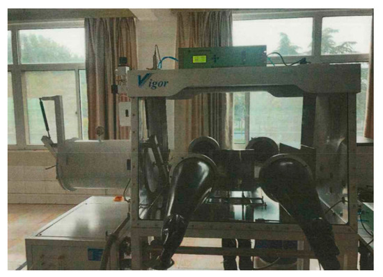
Figure 3.
Test Chamber.
The following are the specific programs:
(1) Water vapor and carbon dioxide are eliminated from the test chamber by replacing the original air with high-purity nitrogen. Replacement rate up to 90%, computed as follows:
where is the original concentration of water vapor in the test chamber; is the concentration after replacement;
(2) To achieve an ultra-low dew point and a carbon dioxide content of less than 1 ppm in the test environment, the circulating purification system is opened after replacement and the gas is purified by adsorption;
(3) Set the water vapor concentration according to the test condition requirements, and compute the formula as follows:
where is the theoretical water vapor concentration required to create the environment; is the temperature in the test chamber; is the relative molecular mass of water vapor; is the theoretical mass of water vapor required to be added; is the value of the barometric pressure in the test chamber; and is the volume of the test chamber;
(4) In this experiment, an airfoil was fabricated using 3D printing (Figure 4). Its internal flow channel design, as seen in Figure 5, is optimized to allow the airfoil to be thoroughly cooled while maintaining a uniform temperature distribution and a stable internal flow field. To prevent the model from frosting during the cooling process under the influence of the environment, an insulation isolation cover is set up in the middle of the test chamber to insulate the airfoil. When the test chamber’s humidity is sufficiently low, liquid nitrogen is injected into the model’s flow channel to circulate and cool it; once the model has reached the desired temperature, the water vapor configuration is introduced into the test chamber, and the concentration of the water vapor is continuously adjusted until it meets the test conditions;
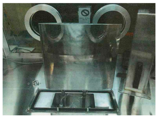
Figure 4.
Wing.
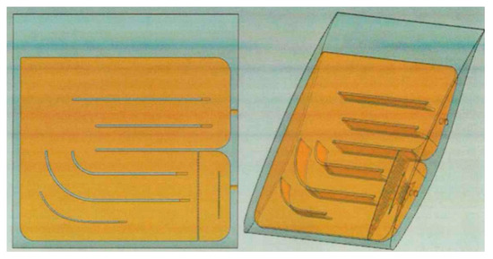
Figure 5.
Design of the airfoil’s internal flow channel.
(5) When the water vapor concentration in the test chamber and the model temperature reach the test requirements, remove the heat preservation isolation cover, and at the same time, control the floating value of water vapor concentration in the test chamber within 2 ppm (Figure 6) to ensure the stability of the test environment.
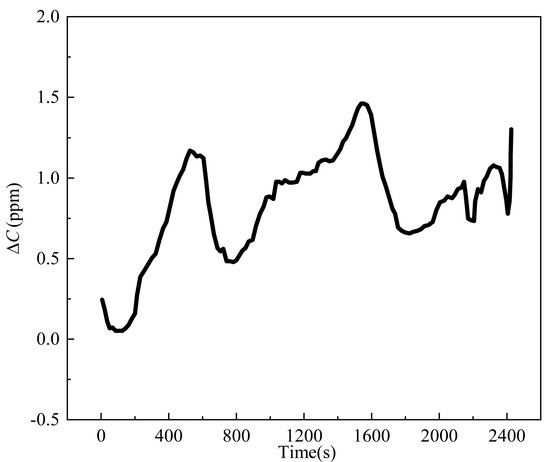
Figure 6.
The floating value of water vapor concentration.
3.1.2. Methods for Measuring Frost
The 3D laser scanning visualization approach was utilized to measure the thickness of the frost layer on the model’s surface and to observe the frost layer evolution process on the supercritical airfoil’s surface in real-time. The measuring device is a handheld laser scanner with an integrated photogrammetric system module that significantly increases the device’s scanning size and accuracy. It has remarkable detail-capturing capabilities, uses a dual-color laser that is red and blue, has a very high resolution, and is less affected by the surrounding environment. It can perform 360° omnidirectional measurements with measurement accuracy of up to 0.02 mm and volume accuracy of up to 0.035 mm. When the model surface water vapor desublimation frost, through the laser equipment to observe the model surface frost thickness, the physical 3D information is converted to digital signals that can be directly processed by the computer, quickly and accurately obtain the frost layer data on the surface of the model.
3.2. Measuring Result
Based on the experimental protocol for water vapor deposition, a cryogenic ultra-low dew point test chamber was designed and constructed. The airfoil was fabricated using 3D printing technology with 316 L stainless steel as the material, featuring a span length of 310 mm and a chord length of 304.8 mm. To ensure the precision of measurement data, a total of 1000 measurement points were carefully arranged on the upper surface of the airfoil. Experiments were conducted under the cases outlined in Table 4, and frost formation phenomena were observed across varying cases.
Table 4.
Test Cases for Water Vapor Deposition.
During the frost formation process via vapor deposition, the frost layer thickness on the upper surface of the airfoil was continuously monitored at two spanwise cross-sections (η1 = 60 mm and η2 = 30 mm from the wingtip) under each test case using 3D laser scanning technology throughout the 0~60 min sampling period. Four sets of experimental data under typical operating cases were analyzed: frost formation data for Case 1 (model temperature: 110 K, water vapor concentration: 6.45 ppm), Case 2 (model temperature: 110 K, water vapor concentration: 21.10 ppm), Case 3 (model temperature: 130 K, water vapor concentration: 19.07 ppm), and Case 4 (model temperature: 150 K, water vapor concentration: 20.19 ppm). Frost thickness distribution data were analyzed at six characteristic time points: 10 min, 20 min, 30 min, 40 min, 50 min, and 60 min. Missing values at specific measurement locations (caused by experimental errors) were replaced with frost thickness values from adjacent non-null data points.
The frost thickness distribution along the flow direction of the airfoil surface under four typical test cases is illustrated in Figure 7, Figure 8, Figure 9 and Figure 10. The results demonstrate that prolonged sublimation duration correlates with progressive frost layer growth, driven by continuous vapor deposition, leading to a gradual increase in thickness over time. Under identical cases, significant differences in frost thickness are observed across different spanwise profiles of the airfoil, while the distribution patterns along the flow direction exhibit similarity. Comparative analysis revealed significant differences among cases: Case 2 exhibited a thicker frost layer and a more complex thickness distribution than Case 1 due to its higher water vapor concentration. Furthermore, despite similar water vapor concentrations in Cases 2, 3, and 4, the elevated temperature in Case 4 resulted in a markedly thinner frost layer compared to Cases 2 and 3, highlighting the inverse relationship between temperature and frost accumulation under comparable humidity levels.
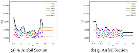
Figure 7.
Frost Thickness Distribution on Airfoil Surface under Case 1.
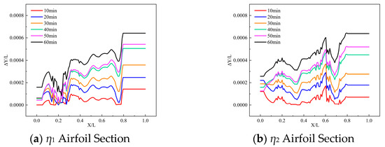
Figure 8.
Frost Thickness Distribution on Airfoil Surface under Case 2.
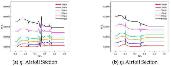
Figure 9.
Frost Thickness Distribution on Airfoil Surface under Case 3.
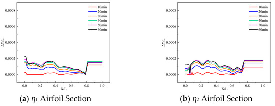
Figure 10.
Frost Thickness Distribution on Airfoil Surface under Case 4.
Therefore, both temperature and water vapor concentration in the experimental environment significantly influence the water vapor deposition characteristics of the airfoil. Subsequent numerical simulations were performed to calculate the frosted airfoil profiles following water vapor deposition under different conditions. The effects of varying experimental environments on the aerodynamic and flow characteristics of the airfoil were analyzed.
4. Effect of the Water Vapor De-Sublimation on the Aerodynamic Characteristics
4.1. Impact Simulation of Frost Layer on Airfoil Aerodynamic Profile
To investigate the coupled effects of model temperature, water vapor concentration, and three-dimensional aerodynamic characteristics on water vapor deposition frosting, experimental data from multiple test cases were systematically analyzed. Given the significant inhomogeneity of surface roughness across different regions of the airfoil surface, to simplify the research problem, this study focuses on the impact of airfoil geometric shape changes induced by frosting on aerodynamic performance. Specifically, based on the experimentally measured frost height data, the macroscopic geometric shape of the frost-accreted airfoil was reconstructed; at this stage, the roughness parameters of the frost surface were not incorporated into the wall boundary conditions, and the influence of frost surface roughness on the airfoil’s aerodynamic performance was temporarily not considered. Frost layer information was chosen at the η1 airfoil section for Cases 1, 3, and 4, and at the η1 and η2 airfoil sections for Case 2. The experimentally acquired frost thickness profiles along the airfoil chord (X/L = 0~1) were mapped onto a baseline airfoil configuration via cubic spline interpolation. This spatial normalization process enabled parametric surface reconstruction, ultimately generating the frost-accreted airfoil morphology dataset for each test condition.
Figure 11 presents the frost-accreted airfoil profile for Case 1 at 60 min, featuring a chord length of L = 0.3048 m. Comparative edge profiles between the frost-accreted (red) and baseline (green) airfoils are shown in Figure 12, with particular emphasis on leading-edge and trailing-edge geometric deviations. A medium-resolution meshing strategy was applied to both the baseline airfoil and the frost-accreted airfoils under four operational cases. The computational grid structure of the baseline airfoil is presented in Figure 13.
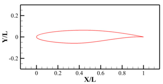
Figure 11.
Frost-Accreted Airfoil Profile.
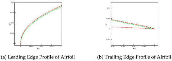
Figure 12.
Comparison of Baseline and Frost-Accreted Airfoil Profiles.
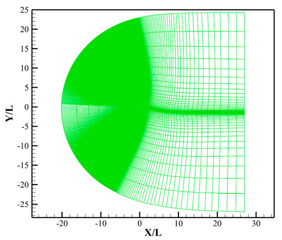
Figure 13.
Baseline Airfoil Grid.
4.2. Influence of Water Vapor Content
- (a)
- Numerical Simulation Results for Tmodel = 110 K and CH2O = 6.45 ppm
Numerical simulations were performed at angles of attack of −2°, 0°, 1°, 2.31°, and 4°. For the numerical solution, the Reynolds-Averaged Navier–Stokes (RANS) method was adopted, with the Spalart–Allmaras model selected as the turbulence model. All computational parameters were maintained identical to those of the validation phase as detailed in Table 3.
Using the baseline airfoil’s numerical simulation results as the baseline, Figure 14 shows the variation rules of the deviations (ΔCL, ΔCD, ΔK, ΔCm) of the lift coefficient CL, drag coefficient CD, lift-to-drag ratio K, and moment coefficient Cm (using the most anterior end of the airfoil as the moment point) between the frost-accreted airfoil and the baseline airfoil with respect to the angle of attack. The legend labels (10, 20, 30, 40, 50, 60 min) correspond to frost-accreted airfoils at six discrete time stages. Analysis revealed that the aerodynamic coefficient deviations demonstrated similar evolutionary trends with increasing frost accretion duration.
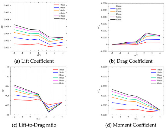
Figure 14.
Aerodynamic Characteristic Deviations Between Frost-Accreted and Baseline Airfoils in Case 1.
As shown in Figure 14a, the lift coefficient deviation ΔCL between the frost-accreted and baseline airfoils demonstrates angle of attack dependence. Specifically, ΔCL exhibits an upward trend with increasing frost accretion duration. The maximum ΔCL of 6.5 × 10⁻³ (7.68% relative deviation) occurs at α = −2° after 60 min frost accretion. All other angles of attack maintained relative deviations below 2% compared to the baseline airfoil.
Figure 14b demonstrates that the drag coefficient deviation ΔCD maintains magnitudes below 1.67 × 10⁻⁴ throughout all computational angles of attack, while all relative deviations remain within 1.3%. ΔCD shows an inverse relation with frost accretion duration at α = −2°, while maintaining positive scaling at other angles of attack.
As evidenced by the ΔK variations in Figure 14c, the frost-accreted airfoil demonstrates progressive increases in lift-to-drag ratio with increasing frost accretion duration at α = −2°, 0°, and 1°. Conversely, a gradual reduction trend emerges at α = 2.31°, while near-identical performance to the baseline airfoil (ΔK < 0.06%) persists at α = 4° despite minor degradation.
Analyzing the variation trend of ΔCm with the angle of attack (Figure 14d), it is found that at the same time, the ΔCm of frost-accreted airfoil gradually decreases as the angle of attack increases; at the same angle of attack, ΔCm increases with the extension of increasing frost accretion duration. All tested angles of attack maintained relative deviations in moment coefficient below 1.6% between frost-accreted and baseline airfoils, with the singular exception of α = −2°.
Figure 15 presents comparative wall pressure coefficient distributions between the frost-accreted and baseline airfoils at different frost accretion durations. A comparison of the wall pressure coefficient curves between the baseline and frosted airfoils demonstrates discernible differences in three specific regions: the upper surface leading edge, X/L = 0.1–0.3, and X/L = 0.65–0.75. The upper surface pressure coefficient at the leading edge exhibits a progressive reduction with increasing frost accretion duration. Simultaneously, the shock wave position demonstrates a weak downstream migration tendency under prolonged frosting conditions. Frost accretion induces pressure redistribution across the entire upper surface, including the anterior, medial, and posterior segments, thereby compromising the airfoil’s global aerodynamic performance.
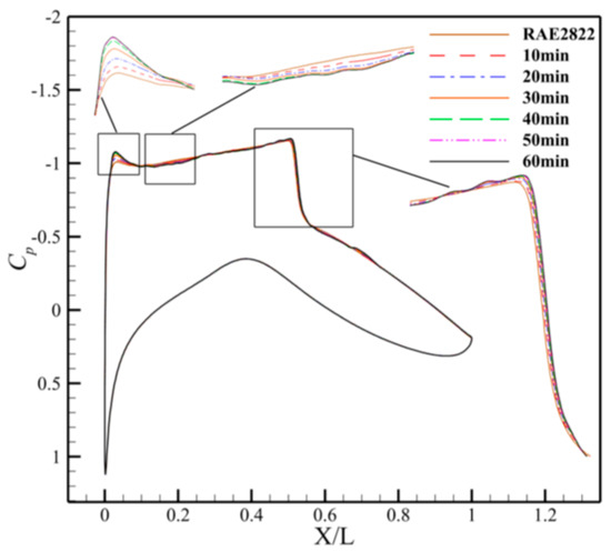
Figure 15.
Wall Pressure Coefficient Distribution of Frost-Accreted Airfoil (Case 1).
Figure 16 presents the Mach number contours at the leading edge regions of baseline and frost-accreted airfoils. Comparative analysis reveals two correlated phenomena: progressive thickening of the frost layer at the leading edge with extended accretion duration and elevated Mach numbers at equivalent streamwise positions.
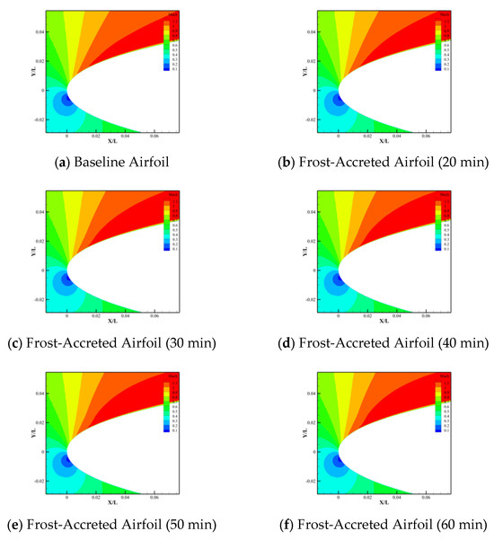
Figure 16.
Mach Number Comparison Between Baseline and Frost-Accreted Airfoils at Leading Edge (Case 1).
Vorticity quantifies the rotational characteristics of fluid motion, defining both the magnitude and direction of velocity field circulation to characterize the intensity and spatial orientation of fluid rotation. In vortex identification methodologies, three prevalent criteria are widely adopted: the Q criterion [29], the λ2 criterion [30], and the Ω criterion [31]. The Q criterion demonstrates broad applicability in fluid dynamic analyses, with implementation advantages stemming from its simplicity and computational efficiency relative to alternative vortex identification methodologies. To further explore the flow field modifications induced by frost accretion, Q criterion contours of both baseline and frost-accreted airfoils at chordwise positions X/L = 0.1~0.7 are comparatively presented in Figure 17. With increasing frost accretion duration, three critical flow modifications are observed: progressive destabilization of the pre-shock flow downstream of X/L = 0.28; slight rearward migration of the shock wave position; and the flow field behind the shock wave undergoes a considerable alteration. This is because the profile change on the airfoil’s upper surface grows as the duration and thickness of frost accretion increase. This alters the flow structure on the airfoil’s surface.
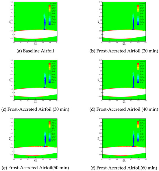
Figure 17.
Q Criterion Contour Comparison Between Baseline and Frost-Accreted Airfoils (Case 1).
- (b)
- Numerical Simulation Results for Tmodel = 110 K and CH2O = 21.10 ppm
Analysis of the variation trends in ΔCL, ΔCD, ΔK, and ΔCm with angle of attack at two distinct spanwise sections under Case 2 (Figure 18 and Figure 19) demonstrates that the influence of frost accretion on aerodynamic characteristics is highly consistent with both angle of attack and frost accretion duration across different spanwise profiles, with deviations remaining within close proximity. This demonstrates spanwise uniformity in frost-induced aerodynamic modifications: under identical conditions, despite localized aerodynamic parameter fluctuations potentially caused by three-dimensional flow effects, the frost-induced modifications in aerodynamic characteristics (CL, CD, K, Cm) exhibit similar quantitative features and evolutionary trends across distinct spanwise profiles.
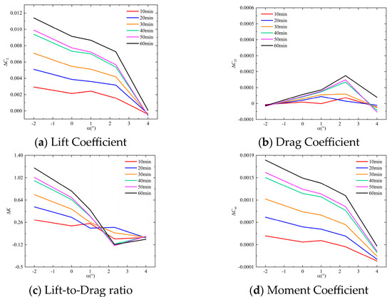
Figure 18.
Aerodynamic Characteristic Deviations Between Frost-Accreted and Baseline Airfoils at the η1 airfoil sections in Case 2.
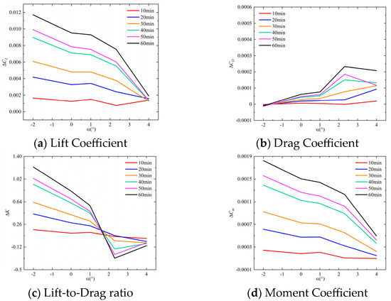
Figure 19.
Aerodynamic Characteristic Deviations Between Frost-Accreted and Baseline Airfoils at the η2 airfoil sections in Case 2.
Comparative analysis of aerodynamic coefficient deviations between Case 2 and Case 1 reveals that frost-induced characteristic deviations in Case 2 exhibit consistent variation patterns with both angle of attack and frost accretion duration when compared to Case 1, with specific manifestations including:
- ΔCL shows a monotonic increase with frost accumulation duration in both cases. Furthermore, comparable ΔCL variation patterns are observed across both cases with increasing angle of attack. During the increase of angle of attack, ΔCL at the same frost duration shows a trend of decreasing, then increasing, and finally decreasing again.
- ΔCD exhibits comparable variation trends with the angle of attack across both cases. During the angle of attack increase from −2° to 2.31°, a consistent ascending tendency in ΔCD is observed. Furthermore, the variation patterns of ΔCD demonstrate similar consistency with increasing frost accretion duration under both conditions.
- Both Case 1 and Case 2 exhibit comparable overall trends in ΔK and ΔCm variations with frost accretion duration and angle of attack.
While maintaining identical model temperatures between Case 1 and Case 2, the latter exhibits elevated water vapor concentration. Although both cases demonstrate highly similar trends in aerodynamic characteristic variations with angle of attack for frost-accreted airfoils, the magnitudes of ΔCL, ΔK, and ΔCm are significantly amplified in Case 2. This confirms that increased water vapor concentration substantially enhances frost layer impacts on aerodynamic performance.
The following important conclusions are drawn from a comparison of the wall pressure coefficient distributions (Figure 20 and Figure 21) and Q criterion contours (Figure 22 and Figure 23) for frost-accreted airfoils at various airfoil sections under Case 2:
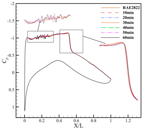
Figure 20.
Wall Pressure Coefficient Distribution of Frost-Accreted Airfoil at the η1 airfoil sections (Case 2).
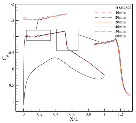
Figure 21.
Wall Pressure Coefficient Distribution of Frost-Accreted Airfoil at the η2 airfoil sections (Case 2).
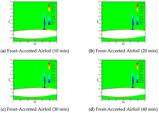
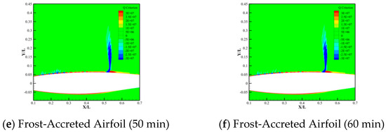
Figure 22.
Q Criterion Contour of Frost-Accreted Airfoil at the η1 airfoil sections (Case 2).
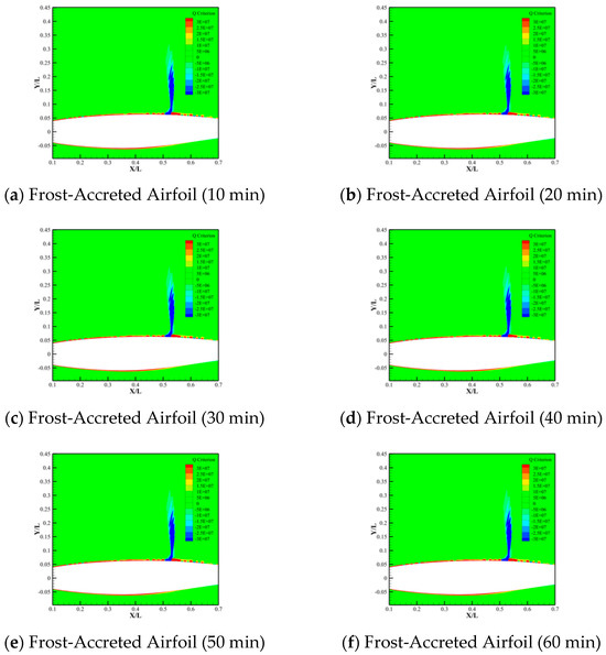
Figure 23.
Q Criterion Contour of Frost-Accreted Airfoil at the η2 airfoil sections (Case 2).
- (1)
- There are distinct differences between the wall pressure coefficient distributions of baseline and frost-accreted airfoils. The baseline airfoil exhibits smooth pressure gradients across the surface, while the frost-accreted airfoils demonstrate enhanced oscillatory characteristics with localized pressure coefficient deviations. Significant variations in the upper surface pressure distribution occur, particularly at airfoil X/L = 0.05~0.4.
- (2)
- Frost accretion modifies the flow field structure on the airfoil’s upper surface, such as fluctuations in the Q-criterion. These alterations arise from frost-induced geometric profile changes, which perturb boundary layer flow characteristics and destabilize the flow. Furthermore, the influence of frost accretion on the airfoil flow structure progressively intensifies with increasing frost accretion duration.
- (3)
- Compared to η2, the spanwise position η1 shows more noticeable frost-induced changes in the flow field structure and pressure distribution, as seen by larger pressure fluctuation amplitudes and more complicated vortex structures.
- (4)
- Streamwise gradients in frost layer thickness critically influence pressure distributions and flow field structures of frost-accreted airfoils. Analysis of the frost layer thickness at the airfoil surface reveals significant pressure coefficient fluctuations at chordwise locations with substantial frost thickness variations. It is evident that the streamwise gradients in frost layer thickness exert a pronounced effect on the modifications to the flow field structure of frost-accreted airfoils.
Case 2 exhibits significantly amplified interference effects on airfoil wall pressure distributions and flow field structures compared to Case 1. This phenomenon originates from the cryogenic, high-humidity experimental conditions in Case 2, where model temperatures fall substantially below the dew point. This induces a drastic elevation of water vapor supersaturation, significantly promoting frost layer formation. The drastic change in the airfoil profile has a substantial effect on the flow field structure.
4.3. Influence of Model Temperature
Using the baseline airfoil’s numerical results as the baseline, analysis of ΔCL, ΔCD, ΔK, and ΔCm variation trends with angle of attack for frost-accreted and baseline airfoils under Cases 3 and 4 (Figure 24 and Figure 25) reveals that frost-induced aerodynamic modifications exhibit highly consistent patterns across all four conditions. Progressive amplification of ΔCL, ΔK, and ΔCm deviations from Case 4 to Case 2 indicates that under similar water vapor concentrations, decreasing model temperatures accelerate desublimation processes and intensify frost layer impacts on aerodynamic characteristics.
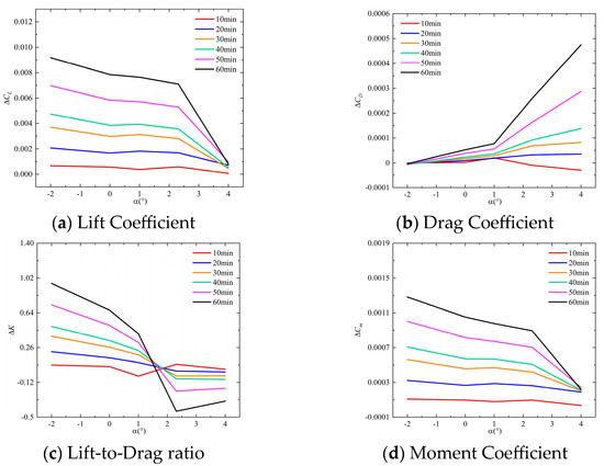
Figure 24.
Aerodynamic Characteristic Deviations Between Frost-Accreted and Baseline Airfoils in Case 3.
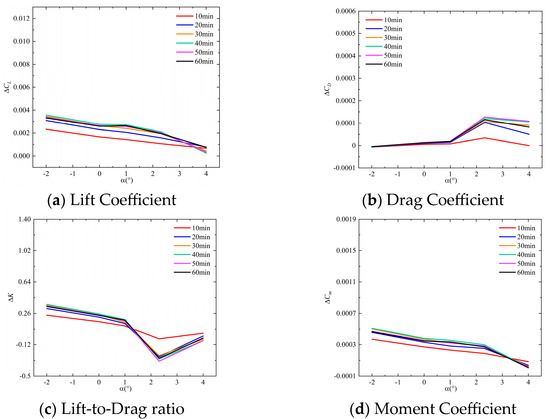
Figure 25.
Aerodynamic Characteristic Deviations Between Frost-Accreted and Baseline Airfoils in Case 4.
The baseline airfoil and frost-accreted airfoils under Cases 3 and 4 are compared in terms of wall pressure coefficient distributions (Figure 26 and Figure 27) and Q criterion contours (Figure 28 and Figure 29). Comparative analysis shows that interference effects on airfoil wall pressure distributions and flow field structures are gradually reduced from Case 2 to Cases 3 and 4, with Case 4 showing the least amount of change. This illustrates how desublimation rate inhibition at high model temperatures under similar water vapor concentrations efficiently inhibits the formation of frost layers.
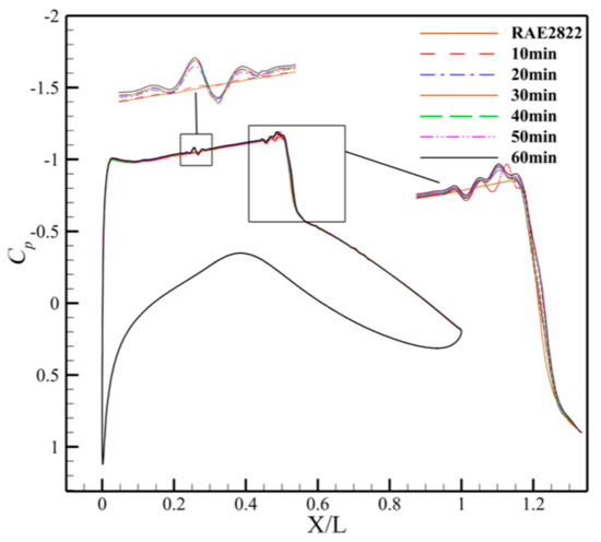
Figure 26.
Wall Pressure Coefficient Distribution of Frost-Accreted Airfoil (Case 3).
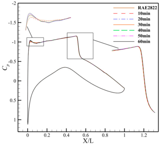
Figure 27.
Wall Pressure Coefficient Distribution of Frost-Accreted Airfoil (Case 4).
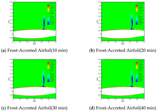
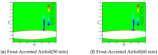
Figure 28.
Q Criterion Contour of Frost-Accreted Airfoil (Case 3).
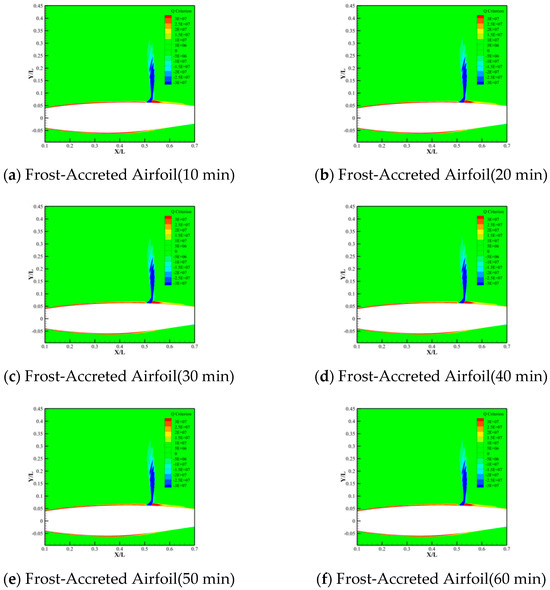
Figure 29.
Q Criterion Contour of Frost-Accreted Airfoil (Case 4).
5. Conclusions
This study constructs a ground testbed based on the characteristics of a cryogenic wind tunnel drying chamber. Optical methods are employed to measure frost thickness distributions on the RAE2822 airfoil surface. Based on the measured results, numerical simulation is then performed to investigate the aerodynamic characteristics of the airfoil. The results indicate that:
- (1)
- Frost layer thickness on the model surface increases with decreasing model temperature, elevated water vapor concentration, and prolonged cryogenic exposure duration.
- (2)
- Water vapor desublimation impacts the lift–drag coefficient, lift-to-drag ratio, and moment coefficient of airfoils. The aerodynamic modifications exhibit significant commonality across conditions: the variation trends of aerodynamic deviations with angle of attack demonstrate notable consistency under different conditions, while the deviations themselves progressively amplify with increasing frost accretion duration.
- (3)
- Water vapor desublimation modifies the airfoil surface pressure distribution and flow field structure, alters boundary layer flow characteristics, and elevates flow instability, thereby inducing rearward displacement of the shock wave. Regions with steeper gradients in frost layer thickness along the flow direction exhibit more pronounced alterations in pressure distribution and flow structure.
- (4)
- Aerodynamic deviations exhibit similarity across different spanwise profiles; however, significant differences in flowfield structures are observed among different spanwise profiles. Cryogenic environments with elevated water vapor concentrations induce drastic supersaturation elevation, accelerating desublimation rates and thereby amplifying aerodynamic modifications and flowfield restructuring.
This study provides insights into the aerodynamic and flowfield modifications induced by water vapor desublimation in cryogenic environments.
However, as a preliminary study, the numerical simulation of the camber morphing wing is limited to the baseline design when the wing camber has not changed since the measurement of the airfoil thickness change is limited to the baseline airfoil. The current findings are helpful for establishing the technical framework for quantitative evaluation in cryogenic conditions, which is important for the real-world application of camber morphing wings.
Author Contributions
Conceptualization, Y.Z., Y.W., B.L., G.L. and J.W.; Methodology, Y.Z., Y.L., Y.W., B.L., G.L. and J.W.; Software, Y.Z., B.H. and Y.L.; Validation, Y.Z., B.H. and Y.L.; Formal analysis, Y.Z., B.H., Y.L. and Y.W.; Investigation, Y.Z., B.H. and Y.L.; Data curation, Y.W.; Writing—original draft, Y.Z. and B.H.; Writing—review & editing, Y.W. and B.L.; Project administration, Y.W. and B.L.; Funding acquisition, Y.W. and B.L. All authors have read and agreed to the published version of the manuscript.
Funding
This research received no external funding.
Data Availability Statement
The original contributions presented in this study are included in the article. Further inquiries can be directed to the corresponding authors.
Conflicts of Interest
The authors declare no conflict of interest.
Correction Statement
This article has been republished with a minor correction to the Data Availability Statement. This change does not affect the scientific content of the article.
References
- Su, J.; Sun, G.; Tao, J. An inverse design method for three-dimensional morphing wings based on deep reinforcement learning. Acta Aerodyn. Aerodyn. Sin. 2024, 42, 84–97. [Google Scholar] [CrossRef]
- Chu, L.; Li, Q.; Gu, F.; Du, X.; He, Y.; Deng, Y. Design, modeling, and control of morphing aircraft: A review. Chin. J. Aeronaut. 2022, 35, 220–246. [Google Scholar] [CrossRef]
- Ajaj, R.M.; Beaverstock, C.S.; Friswell, M.I. Morphing aircraft: The need for a new design philosophy. Aerosp. Sci. Technol. 2016, 49, 154–166. [Google Scholar] [CrossRef]
- Ajaj, R.M. Flight Dynamics of Transport Aircraft Equipped with Flared-Hinge Folding Wingtips. J. Aircr. 2021, 58, 98–110. [Google Scholar] [CrossRef]
- Kota, S.; Flick, P.; Collier, F.S. Flight Testing of FlexFloilTM Adaptive Compliant Trailing Edge. In Proceedings of the 54th AIAA Aerospace Sciences Meeting, San Diego, CA, USA, 4–8 January 2016; AIAA SciTech Forum, American Institute of Aeronautics and Astronautics: Reston, VA, USA, 2016. [Google Scholar]
- Barbarino, S.; Bilgen, O.; Ajaj, R.M.; Friswell, M.I.; Inman, D.J. A Review of Morphing Aircraft. J. Intell. Mater. Syst. Struct. 2011, 22, 823–877. [Google Scholar] [CrossRef]
- Reich, G.; Sanders, B. Introduction to Morphing Aircraft Research. J. Aircr. 2007, 44, 1059. [Google Scholar] [CrossRef]
- Lutz, T.; Kleinert, J.; Waldmann, A.; Koop, L.; Yorita, D.; Dietz, G.; Schulz, M. Research Initiative for Numerical and Experimental Studies on High-Speed Stall of Civil Aircraft. J. Aircr. 2023, 60, 623–636. [Google Scholar] [CrossRef]
- Jimenez-Navarro, C.; Tô, J.B.; Rouaix, C.; Doerffer, P.; Marouf, A.; El Akoury, R.; Braza, M. Morphing Effects on the Aerodynamic Performances of a Supercritical Wing’s Prototype in Transonic Flow Conditions. In Advanced Computational Methods and Design for Greener Aviation; Tuovinen, T., Periaux, J., Knoerzer, D., Bugeda, G., Pons-Prats, J., Eds.; Springer International Publishing: Cham, Switzerland, 2024; pp. 159–174. [Google Scholar]
- Wang, Q.; Qian, W.; Ding, D. A review of unsteady aerodynamic modeling of aircrafts at high angles of attack. Acta Aeronaut. Et Astronaut. Sin. 2016, 37, 2331–2347. [Google Scholar] [CrossRef]
- Waldmann, A.; Ehrle, M.C.; Kleinert, J.; Yorita, D.; Lutz, T. Mach and Reynolds number effects on transonic buffet on the XRF-1 transport aircraft wing at flight Reynolds number. Exp. Fluids 2023, 64, 102. [Google Scholar] [CrossRef]
- Wu, J.; Kong, W.; Li, G.; Tian, S. Progress and prospect on Reynolds number effects of advanced aircraft. Acta Aerodyn. Sin. 2024, 42, 35–59. [Google Scholar] [CrossRef]
- Lai, H.; Chen, W.; Sun, D.; Nie, X.; Zhu, C. The structural design for 0.3 m cryogenic continuous transonic wind tunnel. J. Exp. Fluid Mech. 2020, 34, 89–96. [Google Scholar] [CrossRef]
- Goodyer, M.J. The cryogenic wind tunnel. Prog. Aerosp. Sci. 1992, 29, 193–220. [Google Scholar] [CrossRef]
- Kilgore, R. Evolution and Development of Cryogenic Wind Tunnels. In Proceedings of the 43rd AIAA Aerospace Sciences Meeting and Exhibit, Reno, NV, USA, 10–13 January 2005. [Google Scholar]
- Kilgore, R.A. Cryogenic Wind Tunnels-A Brief Review. In Advances in Cryogenic Engineering; Kittel, P., Ed.; Springer US: Boston, MA, USA, 1994; pp. 63–70. [Google Scholar]
- Kilgore, R.A. Cryogenic Wind Tunnels for Aerodynamic Testing. In Flow at Ultra-High Reynolds and Rayleigh Numbers: A Status Report; Donnelly, R.J., Sreenivasan, K.R., Eds.; Springer: New York, NY, USA, 1998; pp. 66–80. [Google Scholar]
- Wegener, P.P. Cryogenic transonic wind tunnels and the condensation of nitrogen. Exp. Fluids 1991, 11, 333–338. [Google Scholar] [CrossRef]
- Goodyer, M.J.; Kilgore, R.A. High-Reynolds-Number Cryogenic Wind Tunnel. AIAA J. 1973, 11, 613–619. [Google Scholar] [CrossRef]
- Ahlefeldt, T.; Ernst, D.; Goudarzi, A.; Raumer, H.-G.; Spehr, C. Aeroacoustic testing on a full aircraft model at high Reynolds numbers in the European Transonic Windtunnel. J. Sound Vib. 2023, 566, 117926. [Google Scholar] [CrossRef]
- Schauerte, C.; Bosbach, J.; Konrath, R.; Geisler, R.; Philipp, F.; Schreyer, A.-M. Characterization of Transonic Buffet on a Swept Wing by Means of Cryogenic PIV. In Proceedings of the Deutscher Luft- und Raumfahrtkongress 2022, Dresden, Germany, 29 September 2023; pp. 1–10. [Google Scholar]
- Ba, Y.; Chen, Y.; Liu, Y.; Zhang, L. Experimental Investigation of Model Deformation on a High Aspect Ratio Aircraft at Transonic Speeds in ETW. In Proceedings of the 2023 Asia-Pacific International Symposium on Aerospace Technology (APISAT 2023) Proceedings, Singapore, 2 July 2024; pp. 1154–1164. [Google Scholar]
- Gao, J.; Tyrrell, O.K.; Danehy, P.M.; Chan, D.T. Velocity Measurements in the Wake of the Swept Wing Flow Test Model at the National Transonic Facility. In Proceedings of the AIAA SCITECH 2025 Forum, Orlando, FL, USA, 6–10 January 2025; AIAA SciTech Forum, American Institute of Aeronautics and Astronautics: Reston, VA, USA, 2025. [Google Scholar]
- Green, J.; Quest, J. A short history of the European Transonic Wind Tunnel ETW. Prog. Aerosp. Sci. 2011, 47, 319–368. [Google Scholar] [CrossRef]
- Lai, H.; Zhu, C.; Chen, W.; Liao, D.; Sun, D. Key technology for mechanical design in large-scale cryogenic wind tunnel. J. Exp. Fluid Mech. 2022, 36, 19–26. [Google Scholar] [CrossRef]
- Chen, J.; Liu, B.; Chen, W.; Liao, D.; Lai, H. Key technology for model access system in cryogenic wind tunnel. J. Exp. Fluid Mech. 2022, 36, 37–43. [Google Scholar] [CrossRef]
- Haase, W. EUROVAL—An European Initiative on Validation of CFD Codes: Results of the EC/BRITE-EURAM Project EUROVAL, 1990–1992, 1st ed.; 1993 ed.; Vieweg+Teubner Verlag: Wiesbaden, Germany, 1993. [Google Scholar]
- Cook, P.H.; McDonald, M.A.; Firmin, M.C.P. Aerofoil Rae 2822: Pressure Distributions, and Boundary Layer and Wake Measurements; ar 138; AGARD Report: Paris, France, 1 November 1981. [Google Scholar]
- Hunt, J.C.R.; Wray, A.A.; Moin, P. Eddies, streams, and convergence zones in turbulent flows. Cent. Turbul. Res. 1988, 193–208. [Google Scholar]
- Jeong, J.; Hussain, F. On the identification of a vortex. J. Fluid Mech. Digit. Arch. 1995, 285, 69–94. [Google Scholar] [CrossRef]
- Liu, C.; Wang, Y.; Yang, Y.; Duan, Z. New omega vortex identification method. Sci. China Phys. Mech. Astron. 2016, 59, 684711. [Google Scholar] [CrossRef]


Disclaimer/Publisher’s Note: The statements, opinions and data contained in all publications are solely those of the individual author(s) and contributor(s) and not of MDPI and/or the editor(s). MDPI and/or the editor(s) disclaim responsibility for any injury to people or property resulting from any ideas, methods, instructions or products referred to in the content. |
© 2025 by the authors. Licensee MDPI, Basel, Switzerland. This article is an open access article distributed under the terms and conditions of the Creative Commons Attribution (CC BY) license (https://creativecommons.org/licenses/by/4.0/).