A Slip-Based Model Predictive Control Approach for Trajectory Following of Unmanned Tracked Vehicles

Abstract

In the field of tracked vehicle dynamics, studies show that vertical loads are concentrated under road wheels on firm road conditions, allowing slip-based models of tracked vehicles to be designed similar to wheeled vehicle models. This paper proposes a slip-based nonlinear two-track prediction model for model predictive control (MPC), where track forces under road wheels are calculated with a simplification procedure implemented onto shear displacement theory. The study includes a comparative analysis with a kinematic prediction model, examining scenarios such as constant speed cornering and spiral maneuvers. Validation is carried out by comparing the simulation results of the proposed controller with field test data acquired from a five-wheeled tracked vehicle platform, including measurements on asphalt and stabilized road conditions. The results demonstrate that the slip-based model excels in trajectory tracking, with lateral deviations consistently below 0.25 m and typically around 0.02–0.08 m RMS depending on the scenario. By improving the computational efficiency and ensuring precise navigation, this approach offers an advanced control solution for tracked vehicles on firm terrain.

1. Introduction

Motion control studies have gained significant attention, particularly in autonomous vehicles, including robotics and unmanned systems. Tracked vehicles are often characterized by their use of continuous tracks instead of wheels and are widely employed in scenarios involving rough or uneven terrains. However, this paper specifically focuses on the trajectory tracking problem under firm ground conditions, which is also crucial for achieving autonomy in unmanned tracked vehicles (Figure 1). While these vehicles are capable of handling diverse terrains, firm ground presents challenges such as managing high-slip conditions and ensuring accurate trajectory prediction. Our study aims to address these challenges by developing a robust predictive model tailored to firm ground scenarios, enhancing both stability and navigation precision. Various methods have been explored to address these issues, yet a robust predictive model is necessary to enhance navigation accuracy and stability. The trajectory tracking problem is commonly the basis for autonomy and it is handled with many different methods. These approaches can be categorized under following groups:

i.

Classical control methods such as PID control [1];

ii.

Kinematic methods such as pure pursuit and Stanley control [2,3,4];

iii.

Intelligent and learning based methods such as neural network-based control [5];

iv.

Optimization based methods such as model predictive control.

Figure 1. Illustration of an unmanned tracked vehicle platform [6].

Figure 1. Illustration of an unmanned tracked vehicle platform [6].

In tracked vehicle dynamics, methods such as classical PID control offer simplicity but often fail to manage the complex nonlinearities in dynamic systems. Kinematic approaches such as pure pursuit provide basic geometrical path tracking but struggle under conditions with significant slip. Intelligent control methods such as neural networks have potential for adaptability, yet their robustness is still questionable due to limitation with training dataset. Model predictive control (MPC) is effective for handling constraints but becomes computationally challenging when dealing with high-slip scenarios and due to detailed contact mechanics specific to tracked vehicles. These existing methods, while valuable, often do not fully address the challenges at higher speeds, underscoring the need for robust and computationally fast predictive models.

As an optimization-based approach, MPC provides a structured optimal control problem solving technique while conveniently handling the system constraints of linear or non-linear systems. For the trajectory following problem, the MPC approach is extensively used especially in wheeled vehicles. Prediction models for wheeled vehicles show variety, from kinematic single-track models to dynamic two-track models. In high-slip conditions, kinematic single-track models become insufficient for catching the dynamics of actual plant. Therefore, one-track or two-track dynamic models are used introducing the slip of the tires [7,8,9].

Dynamic modelling of tracked vehicles has been widely investigated in the literature, where ride and handling studies are generally covered separately. For ride dynamics, suspension dynamics, track–ground contact relationships, and track wrapping algorithms are mostly studied for both hard and soft soil terrain conditions [10,11,12,13]. In handling studies of these vehicles, accurate modelling constitutes a much more complex phenomenon compared to wheeled vehicles, due to slip occurring through the large contact areas of track pads during skid steer maneuver. Kinematic and dynamic approaches are used in the modelling of these vehicles. In kinematic models, the simplest method includes calculating the instantaneous center of velocity using the track velocities of the vehicle, with slip effects being disregarded [14] (Figure 2a). Additionally, a further improved method for kinematic model is the sliding model, where the instantaneous center is shifted forward due to sliding track characteristics [15,16] (Figure 2b).

In MPC-based trajectory following applications for tracked vehicles, kinematic models are most common due to their simplicity and low computational cost. Zhou et al. [14] employed a torque-driven linearized kinematic model neglecting slip, achieving acceptable results at low speeds with a lightweight test robot using only X, Y, and yaw as controlled states. An EKF-enhanced kinematic model in [17] estimated road and steering resistance, improving lateral tracking by 24% over the basic model in 10–20 km/h off-road tests. In [15], a sliding kinematic model based on the instantaneous turning center was applied to minimize heading deviations for large turning radii. The same authors [16] later updated slip parameters from measured states and applied MPC to the sliding model, outperforming pure pursuit, classical MPC without slip, and the Levenberg–Marquardt method.

When considering the load concentration of the tracks on firm ground, tracked vehicle models can be designed similarly to wheeled vehicle models for slippage calculations under road wheels. A good example for this approach is given in [18], where track force is represented by magic formula as in wheeled vehicles.

Apart from these studies, recent ones have explored diverse trajectory-tracking strategies to enhance the control and efficiency of unmanned vehicles. Reference [19] proposed a polytopic model-based robust MPC for autonomous wheeled vehicles, reducing complexity by using fewer Takagi–Sugeno vertices and adding an H∞ compensation controller for uncertainty and disturbance rejection, validated in Carsim/Simulink. In their extended study [20], they introduced an event-triggered system (ETS) to reduce the communication load while maintaining path-tracking accuracy, validated through hardware-in-the-loop tests. This illustrates the importance of computational efficiency in predictive controllers. Other studies include adaptive MPC for wheel–track hybrid vehicles to address nonlinear and coupled dynamics [21], quartic polynomial planning plus MPC for crawler pavers [22], energy-efficient off-road path planning using a modified A* algorithm [23], online learning and model updating via recursive least squares and Kalman filtering [24], and decoupled adaptive motion control for leader–follower tracked vehicles to maintain precise speed and curvature tracking [25]. These studies collectively highlight the innovative approaches in trajectory tracking, focusing on predictive control strategies to improve the performance and reliability of automated and unmanned vehicle systems across different environments and tasks.

Despite all these studies, there remains a gap in developing robust predictive models for tracked vehicles that can integrate adaptive capabilities and improve decision-making processes under varying environmental conditions. Additionally, most of the studies, especially involving robotic platforms, present low velocities limited to 20 km/h, and the performances of the prediction models are not commonly captured beyond these limits.

To address this gap, we propose a simplified slip-based prediction model for MPC that achieves a practical balance between accuracy and computational efficiency. Unlike purely kinematic methods, which lose accuracy under high-slip conditions, and full dynamic models, which are too computationally demanding for real-time use, the core novelty of this study lies in simplifying the exponential shear displacement formulation (Equation (29)). In the proposed method, the complex integral operation is replaced with an equivalent multiplication of resultant slip velocities and effective contact time [26]. A further analysis shows that particular group of parameters, including the exponential shear displacement function, become insensitive at higher track speeds and slip values. These terms are, therefore, substituted with a constant factor ($K_{simp}$), which yields a mathematically simpler yet bounded error representation of slip dynamics. This innovation not only reduces the computational load but also makes the linearization of the nonlinear model at each MPC step more straightforward and less demanding in the calculation. Building on this principle, the study introduces a torque-driven, slip-based two-track vehicle model that computes slip velocities and contact forces under each wheel, enabling nonlinear MPC to be feasible for real-time trajectory tracking of tracked vehicles operating at higher speeds on firm terrain.

The controller is applied on a plant model, which is taken from [27], and which has extended features through the application of shear displacement theory and built upon the improvements of [28,29,30]. With mentioned modifications, the results of the proposed nonlinear prediction model are compared with the kinematic prediction model in [14], in different scenarios such as (i) cornering maneuvers with increasing speed and (ii) spiral maneuvers with constant speed. Furthermore, a reference trajectory of the created complex test track is used to investigate the performance of the proposed model.

The analyses are conducted in a simulation environment tailored for unmanned driving conditions; however, the controller’s accuracy is validated by replicating the test results from a series of controlled experiments carried out on a five-wheeled tracked vehicle platform, operated in manned mode. These experiments are designed to evaluate the controller’s performance in various scenarios, including low-speed cornering and high-speed maneuvers on an asphalt track, as well as stabilized test parkour. The verification studies involve data from GPS tracking and speed and torque measurements from the sprocket driving shafts, ensuring the controller’s effectiveness and reliability. The postprocessing of these measurements and all methodologies applied in this study is conducted in MATLAB—Simulink R2021b software environments.

The current article comprises eight subsections, including Section 1, which has provided an introduction for the study. In Section 2, the plant model is explained. In Section 3, details of the kinematic-based prediction model are explained. In Section 4, the fundamentals of the proposed nonlinear prediction model are introduced. Additionally, the main contribution of the article is explained here by emphasizing the conducted simplifications in the shear displacement model. In Section 5, the MPC formulation for trajectory tracking problem is described. Results of trajectory following studies are compared in Section 6 for the kinematic-based and proposed slip-based prediction model. In Section 7, the verification studies are discussed, where the collected test data are utilized. Both the vehicle’s measured states and the measurements from the sprocket driving shaft are employed to verify the controller’s output. Finally, the outcomes of the study are summarized in Section 8.

2. Tracked Vehicle Plant Model

The plant model for this study is taken from [27]. The model provides improvements for the transient calculation methods onto past contributions to skid steering tracked vehicle applications. The plant model includes the following features:

(i) Concentrated vertical load under road wheels;

(ii) Discretized cells for track pads under road wheels;

(iii) Shear displacement-based force development;

(iv) Vertical load changes due to longitudinal, lateral acceleration, track pretension, and applied sprocket torques.

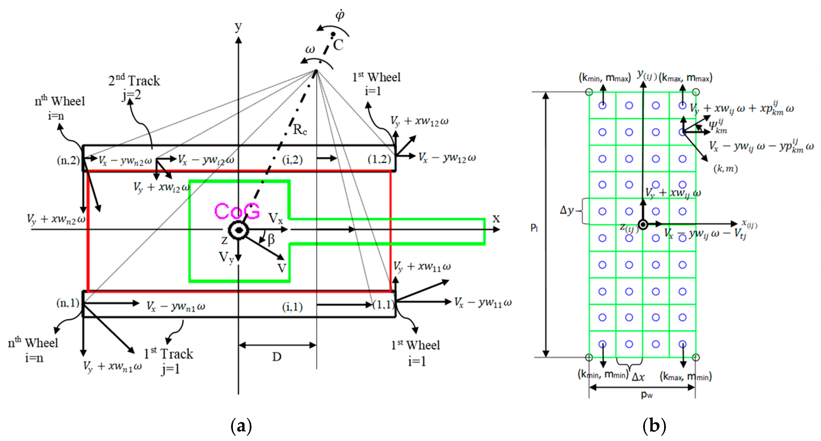
In the model, track pads are discretized to smaller portions and kinematic calculations are performed for each portion (Figure 3b). First, longitudinal, lateral, and resultant slip velocities of each discretized cells are calculated with Equations (1)–(3), where $V_{sxkm}^{ij}$, $V_{sykm}^{ij}$, and $V_{skm}^{ij}$ are the longitudinal, lateral, and resultant slip velocities, respectively; $x{w}_{ij}$ and $y{w}_{ij}$ represent the position of each wheel center in vehicle coordinates; $x{p}_{km}^{ij}$ and $y{p}_{km}^{ij}$ are the positions of the discretized cells in wheel center coordinates; $V_{tj}$ is the velocity of each track.

$$V_{sxkm}^{ij}=V_x-y{w}_{ij}\omega -y{p}_{km}^{ij}\omega -V_{tj},$$

(1)

$$V_{sykm}^{ij}=V_y+x{w}_{ij}\omega +x{p}_{km}^{ij}\omega ,$$

(2)

$$V_{skm}^{ij}=\sqrt{{V_{sxkm}^{ij}}^2+{V_{sykm}^{ij}}^2}.$$

(3)

By integrating the slip velocity along the contact timing of track pads, the slip displacement of each cell can be calculated for both longitudinal and lateral directions. The combination of these displacements gives the overall shear displacement of the cells, as shown in Equation (4), where $j_{km}^{ij}$ corresponds to resultant shear displacement. The integration time bound $∆t_{km}^{ij}$ represents the contact duration of each cell with the ground, which changes with respect to the velocity of the track. Applying the equation used in [31], the shear stress of each track pad cell is calculated in Equation (5), where $F_z^{ij}$ is the vertical load on each wheel, A is the track pad area, $\mu$ is the friction coefficient, and $K$ is the shear deformation modulus.

$$j_{km}^{ij}={\int }_{t-∆t_{km}^{ij}}^t{V}_{skm}^{ij} dt,$$

(4)

$${\tau }_{km}^{ij}={\displaystyle \frac{F_z^{ij}}{A}}\mu (1-e^{-j_{km}^{ij}/K}).$$

(5)

Components of shear forces are summed for each track pad cell in order to calculate total forces under each road wheel in longitudinal ($Q_{xij}$) and lateral ($Q_{yij})$ directions. Additionally, moments created by longitudinal and lateral forces ($M_{xij}$,$M_{yij}$ respectively) are calculated. Finally, equations of motion are calculated in Equations (6)–(8), where $a_x$ is longitudinal acceleration; $a_y$ is lateral acceleration; $R_1$ and $R_2$ are rolling resistance forces of the right and left tracks, respectively; $L_1$ and $L_2$ are the lateral distances of the tracks to the CG of the right and left tracks, respectively.

$$m{a}_x={\sum }_{j=1}^n{\sum }_{i=1}^2{Q}_{xij}+R_1+R_2,$$

(6)

$$m{a}_y={\sum }_{j=1}^n{\sum }_{i=1}^2{Q}_{yij},$$

(7)

$$I_{zz}\dot{\omega }={\sum }_{j=1}^n{\sum }_{i=1}^2\left(M_{xij}+M_{yij}\right)+R_1{L}_1-R_2{L}_2.$$

(8)

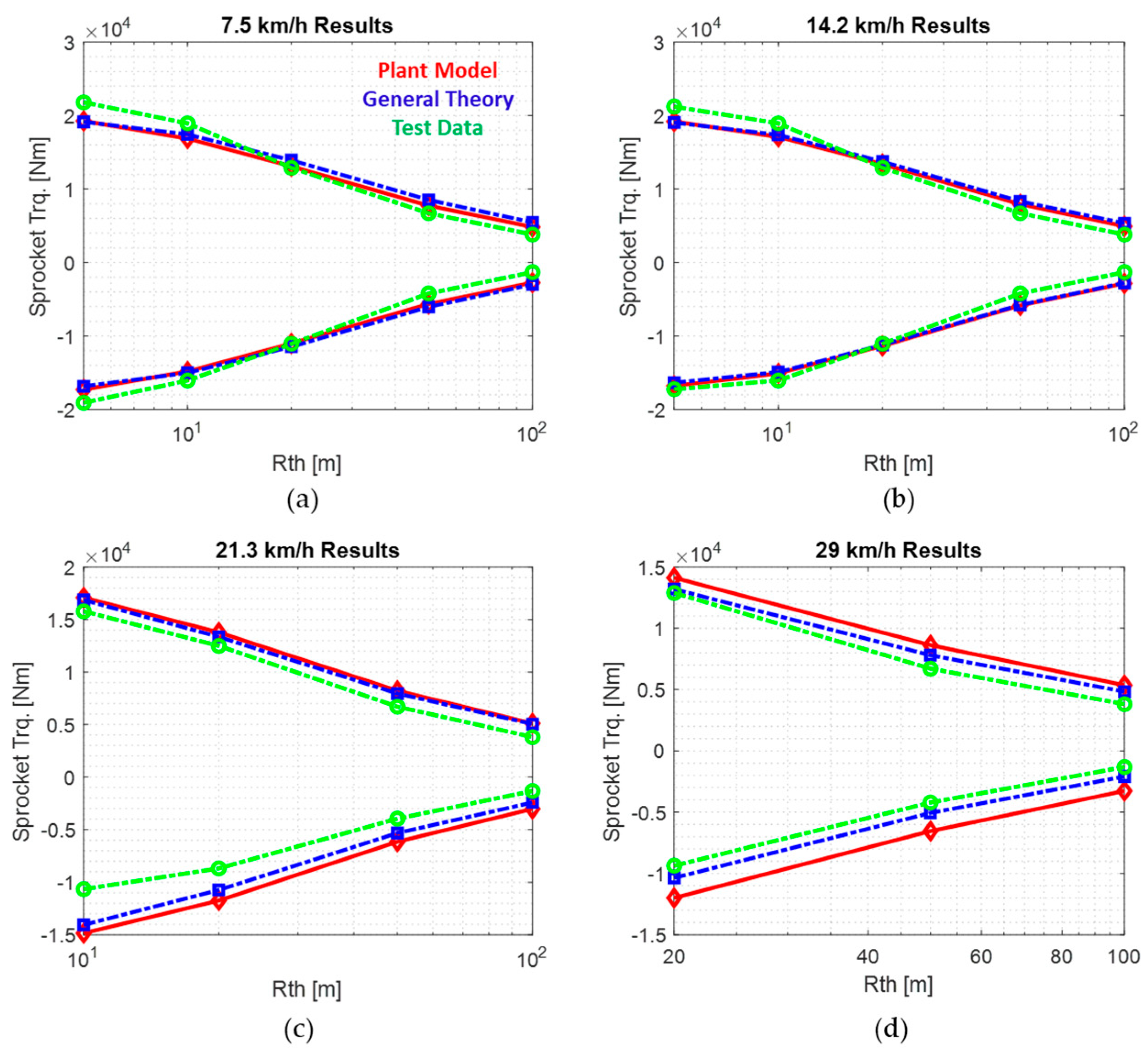
To demonstrate the fidelity of the plant model, sprocket torque results for various turning radii and speeds are compared against the well-known general theory for skid steering presented by Wong et al. [31] and test data in [32,33] obtained from a 25.5 ton tracked vehicle. The comparison, presented in Figure 4, with its numerical data provided in Appendix A, shows that the plant model produces results closely matching the test data, particularly at speeds below 21.3 km/h, with deviations increasing at higher speeds. Nevertheless, the model successfully captures the overall trends and serves as a strong example of a transient tracked vehicle modeling approach that applies state-of-the-art contact force calculations based on the shear displacement method. It should be noted that the general theory results are presented here using the “concentrated load under each road wheel” assumption, one of the approaches investigated by Wong, which is likewise adopted in the plant model.

Building upon the plant model outlined in this section, which covers the essential dynamics of the tracked vehicle, we now advance to the development of predictive models crucial for trajectory tracking. In Section 3, we introduce the kinematic prediction model, offering a simplified approach to forecasting vehicle motion based on geometric and velocity parameters. Subsequently, Section 4 describes the slip-based prediction model, which incorporates the effects of wheel–terrain interactions to enhance predictive accuracy. These models serve as foundational components within the model predictive control framework, which is further explained in Section 5.

3. Kinematic-Based Model as a Foundation for MPC Prediction

In this section, we introduce a kinematic vehicle model as outlined in [14]. This model is used to assess its performance in comparison to the slip-based model described in Section 4. Both models operate as nonlinear prediction tools within the model predictive control framework, enabling predictions of vehicle motion to facilitate the trajectory following control of the plant model described in Section 2. The integration of these models within the MPC formulation is further detailed in Section 5.

The layout of the model is presented in Figure 2a. The positions in longitudinal and lateral coordinates ($x_c, y_c$) and the yaw angle ($\psi$) of the vehicle are the main states of the model, where the velocities of the outer and inner tracks ($v_o$,$v_i$) are the main inputs of the system initially. Nonlinear equations for vehicle motion can be written with the following nonholonomic form, where $T$ refers to the thread of the vehicle.

$$\left[\begin{array}{c}\dot{x_c}\\ \dot{y_c}\\ \dot{\psi }\end{array}\right]=\left[\begin{array}{cc}0.5\cos \left(\psi \right)& 0.5\cos \left(\psi \right)\\ 0.5\sin \left(\psi \right)& 0.5\sin \left(\psi \right)\\ 1/T& -1/T\end{array}\right]\left[\begin{array}{c}{v}_o\\ v_i\end{array}\right].$$

(9)

To extend the given definition and apply the sprocket torques as inputs of the system, tracked vehicle force equations and kinematic relationships can be used. Dynamics at the sprocket level can be defined as in Equation (10), where, $F_{o-i}$ defines the required traction force (Equation (11)), which comprises resistance due to (i) longitudinal motion $F_{Res}$, and (ii) the so-called turning resistance moment—$M_{Steer}$, while the rest of the components belong to (iii) translational and (iv) rotational inertial forces (${\displaystyle \frac{\delta m_{veh}·\dot{v_C}}{2}}$ and ${\displaystyle \frac{I_{zz}·\ddot{\psi }}{T}}$, respectively).

$$J·{{\dot{\omega }}_{spr}}_{o-i}={{\tau }_{spr}}_{o-i}-F_{o-i}·r_{spr}.$$

(10)

$$F_{o-i}={\displaystyle \frac{F_{Re{s}_{o-i}}+\delta m_{veh}·\dot{v_c}}{2}}\pm {\displaystyle \frac{M_{Steer}+I_{zz}·\ddot{\psi }}{T}}.$$

(11)

The turning resistance moment ($M_{Steer}$) [31], steering resistance force ($F_{Steer}$), and effective lateral friction coefficient (${\mu }_t)$ [34] definitions are given in Equations (12) and (13).

$$F_{Steer}={\displaystyle \frac{M_{Steer}}{T}}={\displaystyle \frac{{\mu }_t·m·g·L}{4·T}},$$

(12)

$${\mu }_t={\mu }_{max}·{\left(0.925+0.15·{\displaystyle \frac{R}{T}}\right)}^{-1}.$$

(13)

Combining Equations (10) and (11), sprocket level equations take the following form:

$$J·{{\dot{\omega }}_{spr}}_{o-i}={{\tau }_{spr}}_{o-i}-\left({\displaystyle \frac{{F_{Res}}_{o-i}}{2}}+{\displaystyle \frac{\delta m_{veh}·\dot{V_c}}{2}}\pm {\displaystyle \frac{I_{zz}·\ddot{\psi }}{T}}\pm F_{Steer}\right)·r_{spr}.$$

(14)

Combined kinematic equations of motion of the tracked vehicle are obtained as in Equations (15)–(19):

$$\dot{x}=Ax+Bu,$$

(15)

$$x={\left[\begin{array}{cc}\begin{array}{ccc}{x}_c& y_c& \psi \end{array}& \begin{array}{ccc}{{\omega }_{spr}}_o& {{\omega }_{spr}}_i& v_c\end{array}\end{array}\right]}^{\prime },$$

(16)

$$A=\left[\begin{array}{cccccc}0& 0& 0& 0& 0& 0\\ 0& 0& 0& 0& 0& 0\\ {\displaystyle \frac{r}{2}}\mathrm{c}\mathrm{o}\mathrm{s}\left(\psi \right)& {\displaystyle \frac{r}{2}}\mathrm{c}\mathrm{o}\mathrm{s}\left(\psi \right)& 0& 0& 0& 0\\ {\displaystyle \frac{r}{2}}\mathrm{s}\mathrm{i}\mathrm{n}\left(\psi \right)& {\displaystyle \frac{r}{2}}\mathrm{s}\mathrm{i}\mathrm{n}\left(\psi \right)& 0& 0& 0& 0\\ {\displaystyle \frac{r}{T}}& {\displaystyle \frac{r}{T}}& 0& 0& 0& 0\\ {\displaystyle \frac{r}{2}}& {\displaystyle \frac{r}{2}}& 0& 0& 0& 0\end{array}\right],$$

(17)

$$B=r_{spr}·\left[\begin{array}{cccccc}{\displaystyle \frac{k_1}{r_{spr}}}& -k_1& -k_1& {\displaystyle \frac{k_2}{r_{spr}}}& -k_2& -k_2\\ {\displaystyle \frac{k_2}{r_{spr}}}& -k_2& -k_2& {\displaystyle \frac{k_1}{r_{spr}}}& -k_1& -k_1\\ 0& 0& 0& 0& 0& 0\\ 0& 0& 0& 0& 0& 0\\ 0& 0& 0& 0& 0& 0\\ 0& 0& 0& 0& 0& 0\end{array}\right],$$

(18)

$$u={\left[\begin{array}{cc}\begin{array}{ccc}{\tau }_{sp{r}_o}& {F_{Res}}_o& {F_{SteerRes}}_o\end{array}& \begin{array}{ccc}{{\tau }_{spr}}_i& {F_{Res}}_i& {F_{SteerRes}}_i\end{array}\end{array}\right]}^{\prime },$$

(19)

where $k_1$ and $k_2$ in Equations (17) and (18) comprise terms related to inertial effects, such as the inertia of driveline $J$ and yaw inertia of the vehicle $J_c$, as shown in Equations (20) and (21).

$$k_1={\displaystyle \frac{1}{2}}\left({\displaystyle \frac{1}{J+\delta m_{veh}·r_{spr}^2}}+{\displaystyle \frac{1}{J+\frac{2·J_c·r_{spr}^2}{T^2}}}\right),$$

(20)

$$k_2={\displaystyle \frac{1}{2}}\left({\displaystyle \frac{1}{J+\delta m_{veh}·r_{spr}^2}}-{\displaystyle \frac{1}{J+\frac{2·J_c·r_{spr}^2}{T^2}}}\right).$$

(21)

In concluding the vehicle model introduced in this section, this approach provides a foundational basis for the vehicle motion obtained by applying the kinematic laws. To facilitate its application within the MPC framework, we linearize the nonlinear state matrices by their Jacobians. This linearization process yields discretized state representations, essential for predicting future states over the defined prediction horizon. These specific procedures will be explained thoroughly in Section 5.

4. Development of a Simplified Slip-Based Model as a Foundation for MPC Prediction

This section introduces the core research contribution of this study—a simplified slip-based nonlinear prediction model specifically designed for model predictive control of tracked vehicles. Traditional shear displacement models often involve computationally intensive integrals, making them less practical for real-time applications. The proposed model addresses this challenge by implementing further simplifications, enhancing computational efficiency while maintaining effective tracking performance. The simplified model is verified later through a comparison with the full nonlinear shear-displacement-based plant model. As a remainder, this section, as well as Section 3, establish the fundamentals of the prediction models. Next, these models are utilized in the MPC framework as the derivations that will be explained in Section 5.

Differing from kinematic models, the proposed model includes the contact force generation characteristics of track pads. Assuming that the vertical load under track pads is concentrated under road wheels, calculations can be performed based on point contact force generation as in wheeled vehicle applications. Therefore, slip velocities are calculated for each road wheel location with kinematic relations. Shear forces developed by the pads are estimated for longitudinal and lateral directions. Finally, equations of motion based on these forces are constructed.

As described in Equations (4) and (5), calculating shear forces in tracked vehicles typically involves integrating the slip velocity over the contact time, a process that can be computationally intensive and challenging to linearize. To address this, our study applies simplifications in track force estimation to develop a more efficient prediction model. As stated in [28], shear displacement can be approximated with the multiplication of combined slip and average contact times, as in Equation (22), where $j_{ij}$ defines the shear displacement under each road wheel, $V_{S-ij}$ defines the resultant slip velocity, and $t_{avg}$ is the average contact time under road wheels. Notice that this equation is a simplified version, where $t_{avg-ij}$ is calculated by dividing the contact length ($L_{con-i})$ under road wheels by the track velocity, as in Equation (23). Here, $l_i$ is the vectoral distance of the i^th road wheel to the CG. Therefore,$L_{con-i}$ defines the distance of the road wheel to first road wheel.

$$j_{ij}=V_{S-ij}·t_{avg-ij},$$

(22)

$$t_{avg-ij}={\displaystyle \frac{L_{con-i}}{V_{tj}}}={\displaystyle \frac{l_1-l_i}{V_{tj}}}.$$

(23)

The slip ratio under each wheel can be expressed with Equations (24)–(26).

$$s_{x-ij}={\displaystyle \frac{V_{sx-ij}}{r_{spr}·{\omega }_{sp{r}_j}}},$$

(24)

$$s_{y-ij}={\displaystyle \frac{V_{sy-ij}}{r_{spr}·{\omega }_{sp{r}_j}}},$$

(25)

$$s_{ij}={\displaystyle \frac{\sqrt{V_{sx-ij}^2+V_{sy-ij}^2}}{r_{spr}·{\omega }_{spr}}}={\displaystyle \frac{V_{s-ij}}{r_{spr}·{{\omega }_{spr}}_j}}.$$

(26)

Utilizing Equations (24)–(26), components of the forces in longitudinal and lateral directions can be defined as in Equations (27) and (28), where $F_{ij}$ is the resultant force (Equation (29)), which refers to the well-known shear displacement approach [31].

$$F_{x-ij}=F_{ij}·{\displaystyle \frac{-s_{x-ij}}{s_{ij}}}=F_{ij}·{\displaystyle \frac{-V_{sx-ij}}{V_{s-ij}}},$$

(27)

$$F_{y-ij}=F_{ij}·{\displaystyle \frac{-s_{y-ij}}{s_{ij}}}=F_{ij}·{\displaystyle \frac{-V_{sy-ij}}{V_{s-ij}}},$$

(28)

$$F_{ij}=F_{z-ij}·\mu ·\left(1-e^{-{\displaystyle \frac{j_{ij}}{K}}}\right).$$

(29)

The last term in Equation (29) is the exponential function, and by combining Equations (22) and (23), the following definition is obtained:

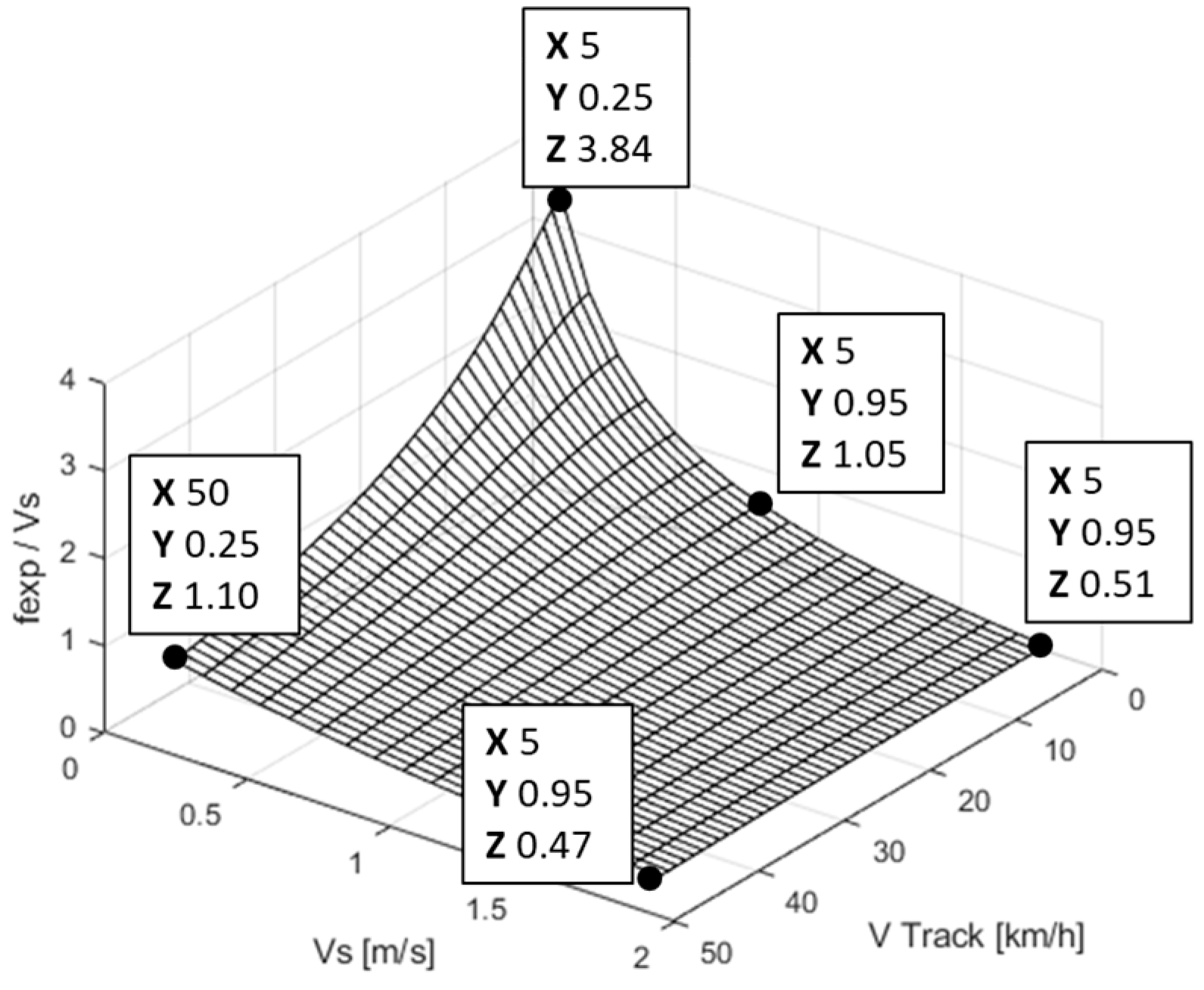
$$f_{exp-ij}=1-e^{-{\displaystyle \frac{j_{ij}}{K}}}=1-e^{-{\displaystyle \frac{V_{s-ij}/V_{tj}}{K/L_{contact-i}}}}.$$

(30)

Combining Equations (27)–(30), the force equations become Equations (31) and (32).

$$F_{x-ij}=-V_{sx-ij}·F_{z-ij}·\mu ·\left({\displaystyle \frac{f_{exp-ij}}{V_{s-ij}}}\right),$$

(31)

$$F_{y-ij}=-V_{sy-ij}·F_{z-ij}·\mu ·\left({\displaystyle \frac{f_{exp-ij}}{V_{s-ij}}}\right).$$

(32)

Analyzing the effect of change of $V_{s-ij}$ and the $V_{tj}$ in change of $f_{exp}/V_s$, the surface in Figure 5 is obtained for the mid road wheel. The increases in $V_{s-ij}$ and $V_{tj}$ parameters lead $f_{exp}/V_s$ to operate on an almost planar surface and become insensitive to their increase. This feature can be used in the simplification of the prediction model. Instead of an exact calculation of this factor, a constant value can be applied, so that the calculation effort in track forces decreases. Therefore, calculations of longitudinal and lateral forces can be approximated with Equations (33) and (34). Finally, the layout of the proposed model can be constructed as in Figure 6. The method used to calculate the vertical load under each wheel is explained in Appendix B.

$$F_{x-ij}\approx -V_{sx-ij}·F_{z-ij}·\mu ·K_{simp},$$

(33)

$$F_{y-ij}\approx -V_{sy-ij}·F_{z-ij}·\mu ·K_{simp}.$$

(34)

The longitudinal slip velocities under the i^th road wheel on the right side and left sides of the vehicle are calculated using Equations (35) and (36).

$$V_{sx-iR}=v_x+{\displaystyle \frac{T}{2}}·\dot{\psi }-{\omega }_{sp{r}_R}·r_{spr},$$

(35)

$$V_{sx-iL}=v_x-{\displaystyle \frac{T}{2}}·\dot{\psi }-{\omega }_{sp{r}_L}·r_{spr}.$$

(36)

Moments created by longitudinal forces on the right and left sides are then calculated according to Equations (37) and (38), where $F_{x-iR}$ and $F_{x-iL}$ are the transmitted longitudinal forces under the i^th wheel on the right and left sides, respectively.

$$M_{x-iR}={\displaystyle \frac{T}{2}}·\sum _{i=1}^5{F}_{x-iR},$$

(37)

$$M_{x-iL}=-{\displaystyle \frac{T}{2}}·\sum _{i=1}^5{F}_{x-iL}.$$

(38)

The lateral slip velocities under the i^th road wheel on the right side and left side of the vehicle are calculated using Equation (39).

$$V_{sy-iR}=V_{sy-iL}=v_y+l_i·\dot{\psi }.$$

(39)

Moments created by lateral forces on the right and left sides are then calculated according to Equations (40) and (41), where $F_{y-iR}$ and $F_{y-iL}$ are transmitted lateral forces under the i^th wheel on the right and left sides, respectively.

$$M_{y-iR}=\sum _{i=1}^5{F}_{y-iR}·l_i,$$

(40)

$$M_{y-iL}=\sum _{i=1}^5{F}_{y-iL}·l_i.$$

(41)

Using the force and moment calculations, state calculations for the longitudinal and lateral velocities of the vehicle in body coordinates and yaw velocity are conducted with Equations (42)–(44).

$${\dot{v}}_x={\displaystyle \frac{\sum _{i=1}^5\sum _{j=1}^2{F}_{x-ij}-F_{Res}}{m}}+v_y·\dot{\psi },$$

(42)

$${\dot{v}}_y={\displaystyle \frac{\sum _{i=1}^5\sum _{j=1}^2{F}_{y-ij}}{m}}-v_x·\dot{\psi },$$

(43)

$$\ddot{\psi }={\displaystyle \frac{M_{x-iR}+M_{x-iL}+M_{y-iR}+M_{y-iL}}{I_{zz}}}.$$

(44)

Velocities of the vehicle in global coordinates are calculated by applying appropriate transformations, as shown in Equations (45)–(47). The integration of these parameters over time provides the calculation of position states ($x$, $y$ and $\psi$) given in Equation (51).

$$V_x=v_x·\cos \left(\psi \right)-v_y·\sin \left(\psi \right),$$

(45)

$$V_y=v_x·\sin \left(\psi \right)+v_y·\cos \left(\psi \right),$$

(46)

$$\dot{\psi }=\omega .$$

(47)

Finally, states for sprocket speeds are calculated by differential equations given in Equations (48) and (49).

$${\dot{\omega }}_{sp{r}_R}={\displaystyle \frac{{{\tau }_{spr}}_R-\sum _{i=1}^5{F}_{x-iR}·r_{spr}}{J}},$$

(48)

$${\dot{\omega }}_{sp{r}_L}={\displaystyle \frac{{{\tau }_{spr}}_L-\sum _{i=1}^5{F}_{x-iL}·r_{spr}}{J}}.$$

(49)

The states and inputs of the nonlinear model are summarized in Equations (50)–(52).

$$\dot{x}={\left[\begin{array}{cc}\begin{array}{cc}\begin{array}{cc}{V}_x& V_y\end{array}& \begin{array}{cc}\dot{\psi }& {\dot{v}}_x\end{array}\end{array}& \begin{array}{cc}\begin{array}{cc}{\dot{v}}_y& \ddot{\psi }\end{array}& \begin{array}{cc}{\dot{\omega }}_{sp{r}_R}& {\dot{\omega }}_{sp{r}_L}\end{array}\end{array}\end{array}\right]}^{\prime },$$

(50)

$$x={\left[\begin{array}{cc}\begin{array}{cc}\begin{array}{cc}x& y\end{array}& \begin{array}{cc}\psi & v_x\end{array}\end{array}& \begin{array}{cc}\begin{array}{cc}{v}_y& \dot{\psi }\end{array}& \begin{array}{cc}{\omega }_{sp{r}_R}& {\omega }_{sp{r}_L}\end{array}\end{array}\end{array}\right]}^{\prime },$$

(51)

$$u={\left[\begin{array}{cc}\begin{array}{cc}{{\tau }_{spr}}_R& {{\tau }_{spr}}_L\end{array}& \begin{array}{cc}{F_{Res}}_R& {F_{Res}}_L\end{array}\end{array}\right]}^{\prime }.$$

(52)

In the MPC structure, ${\tau }_{sp{r}_o}$ and ${\tau }_{sp{r}_i}$ are designed as manipulated variables, whereas resistance forces are fed to the system as calculated inputs. The reference trajectory is fed to the system in terms of its longitudinal and lateral positions and yaw angle, as in the kinematic-based prediction model: $x_{ref}=\left[{\begin{array}{ccc}{X}_{ref}& Y_{ref}& \psi \end{array}}_{ref}\right]$.

In this section, we develop a simplified slip-based model. This model incorporates slip dynamics, addressing the limitations of the kinematic model. The next section provides a procedure for how these models are utilized to predict future vehicle states, formulate control objectives, and implement constraints to achieve optimal trajectory tracking performance.

5. MPC Problem Formulation

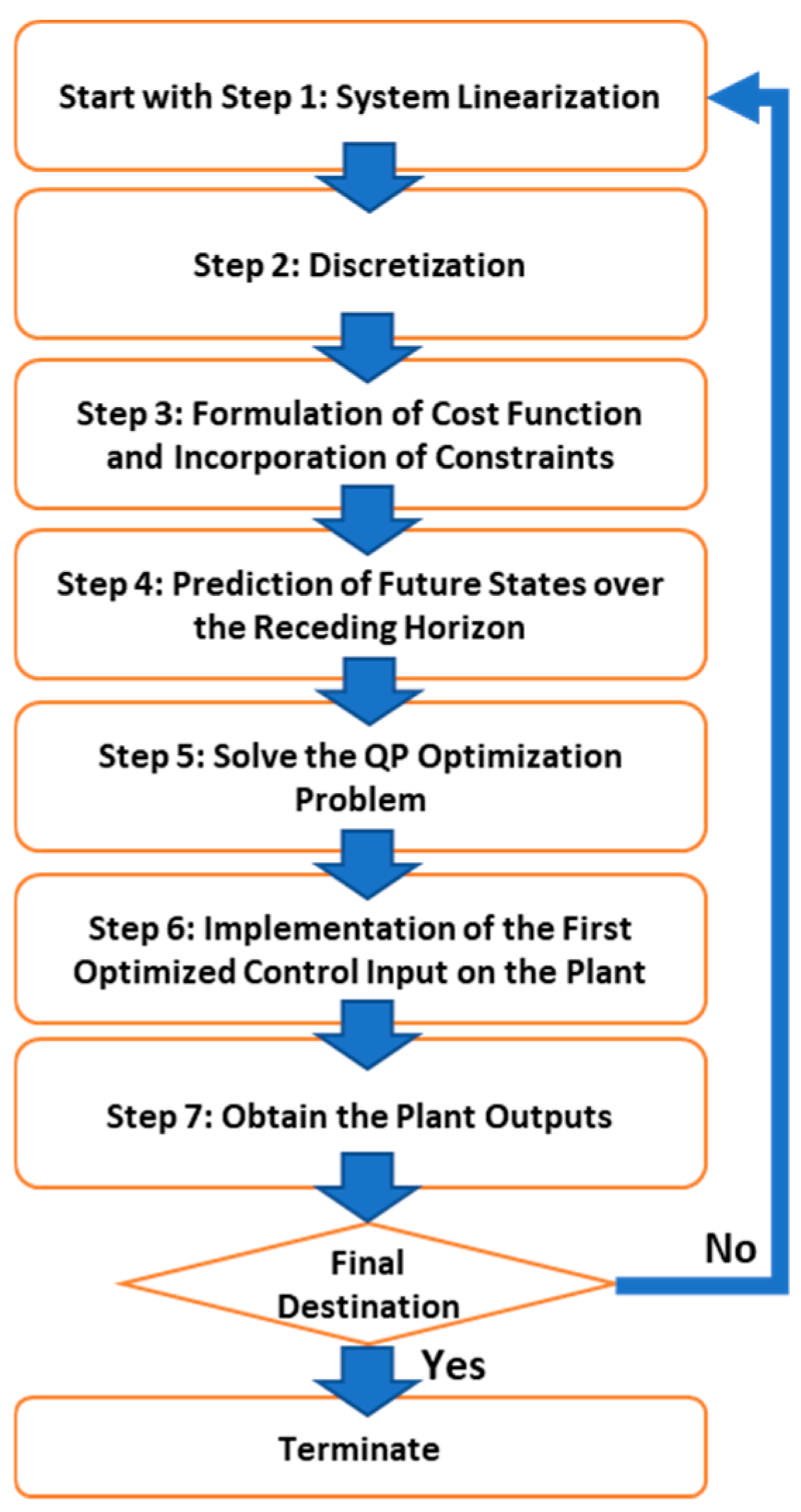
In this section, we detail the model predictive control (MPC) formulation, utilizing both the kinematic model from Section 3 and the slip-based model from Section 4 as prediction models for trajectory tracking. The nonlinear prediction models used in this study (kinematic and slip-based) are linearized at each controller sampling instant (Ts = 0.05 s) about the current measured states and latest control inputs. This yields the updated Jacobian matrices $A_J$ and $B_J$ of the system dynamics with respect to states and inputs in Equations (62)–(65). These continuous-time Jacobians are then discretized using the Euler method (Equations (66)–(68)) to produce the local linear prediction model in discrete-time state–space form. Based on this model, the MPC cost function is formulated to penalize deviations from the reference trajectory and excessive control changes over a prediction horizon N = 20 (1 s look-ahead) and a control horizon M = 2 (0.1 s control window). The resulting QP problem is solved using MATLAB’s fmincon function; only the first control action of the optimized sequence is applied to the plant before the horizon is shifted forward and the procedure repeated. An analysis for computational efficiency is introduced later in Section 6.2, with a sensitivity analysis of these specific MPC parameters providing the timing headroom for the calculation of each step-in solution of the MPC problem over a specific scenario. To facilitate the MPC design, Figure 7 presents a flowchart of this process, showing the mentioned process sequence.

To start with the derivation, generalized discrete state space calculations can be given with the following equations, where k is the stage number of the problem:

$$x\left(k+1\right)=Ax\left(k\right)+Bu\left(k\right),$$

(53)

$$y\left(k\right)=Cx\left(k\right)+Du\left(k\right).$$

(54)

States for the vehicle, which follow the trajectory perfectly, are calculated by the function given in Equation (55). The inputs of this function are the reference state vector (Equation (56)) and the reference manipulated vector $u_{ref}$ (Equation (57)).

$${\dot{x}}_{ref}=f\left(x_{ref},u_{ref}\right).$$

(55)

$$x_{ref}=\left[\begin{array}{ccc}{X}_{ref}& Y_{ref}& {\psi }_{ref}\end{array}\right],$$

(56)

$$u_{ref}=\left[\begin{array}{cc}{\tau }_{Spr-R}& {\tau }_{Spr-L}\end{array}\right],$$

(57)

Actual states of the vehicle are calculated by Equation (58).

$$\dot{x}=f\left(x,u\right)=Ax+Bu.$$

(58)

Nonlinear state equations are linearized with Taylor series expansion, as in Equation (59).

$${\dot{x}}_{ref}\approx f\left(x_{ref},u_{ref}\right)+{\displaystyle \frac{df}{dx}}|\left(x-x_{ref}\right)+{\displaystyle \frac{df}{du}}|\left(u-u_{ref}\right).$$

(59)

Subtracting Equations (58) and (59), Equations (60) and (61) can be obtained. $A_J$ and $B_J$ are Jacobian matrices with respect to ($x-x_{ref})$ and $(u-u_{ref})$, respectively (Equations (62) and (63)).

$$\dot{\tilde{x}}=\dot{x}-{\dot{x}}_{ref}\approx f\left(x,u\right)-f\left(x_{ref},u_{ref}\right)-{\displaystyle \frac{df}{dx}}\left|\left(x-x_{ref}\right)-{\displaystyle \frac{df}{du}}\right|\left(u-u_{ref}\right),$$

(60)

$$\dot{\tilde{x}}=A_J\tilde{x}+B_J\tilde{u},$$

(61)

$$A_J\left(t\right)={\displaystyle \frac{df}{dx}}|\left(x-x_{ref}\right),$$

(62)

$$B_J\left(t\right)={\displaystyle \frac{df}{du}}|\left(u-u_{ref}\right).$$

(63)

Using the state matrices in Equations (17) and (18), Jacobian matrices of the kinematic-based nonlinear model (Section 3) are computed by taking the partial derivatives of the system dynamics with respect to the state vector x in Equation (16) and the input vector u in Equation (19). The same linearization procedure is applied to the slip-based prediction model, where the Jacobians are computed from the nonlinear state Equations (42)–(49) with respect to states given in Equation (51) and the input vector in Equation (52). The resulting continuous-time Jacobians $A_J$ and $B_J$ define the local linear approximation of the nonlinear dynamics at a given operating point. Based on these calculations, the explicit form of $A_J$ is given in Equation (64), while $B_J$ is expressed in Equation (65) for the slip-based prediction model. The detailed, term-by-term partial derivatives used to construct these matrices are provided in Appendix C, enabling direct traceability from the nonlinear state equations to the elements of $A_J$ and $B_J$.

$$A_J=\left[\begin{array}{ccccc}0& 0& -v_y\cos \left(\psi \right)-v_x\sin \left(\psi \right)& \cos \left(\psi \right)& -\sin \left(\psi \right)\\ 0& 0& v_x\cos \left(\psi \right)-v_y\sin \left(\psi \right)& \sin \left(\psi \right)& \cos \left(\psi \right)\\ 0& 0& 0& 0& 0\\ 0& 0& 0& -{\displaystyle \frac{\left(F_{res}+F_{z-sum}{K}_{simp}\right)}{m}}& \dot{\psi }\\ 0& 0& 0& \dot{-\psi }& -{\displaystyle \frac{K_{simp}{F}_{z-sum}}{m}}\\ 0& 0& 0& {\displaystyle \frac{K_{simp}T\left(F_{zL-sum}-F_{zR-sum}\right)}{2·I_{zz}}}& {\displaystyle \frac{-K_{simp}{\sum }_{i=1}^5\left(F_{z-iR}{l}_i+F_{z-iL}{l}_i\right)}{I_{zz}}}\\ 0& 0& 0& {\displaystyle \frac{K_{simp}{r}_{spr}{F}_{zR-sum}}{J}}& 0\\ 0& 0& 0& {\displaystyle \frac{K_{simp}{r}_{spr}{F}_{zL-sum}}{J}}& 0\end{array}\right.\left.\begin{array}{ccc}0& 0& 0\\ 0& 0& 0\\ 1& 0& 0\\ {\displaystyle \frac{2m{v}_y+K_{simp}T\left(F_{zL-sum}-F_{zR-sum}\right)}{2m}}& {\displaystyle \frac{K_{simp}{r}_{spr}{F}_{zR-sum}}{m}}& {\displaystyle \frac{K_{simp}{r}_{spr}{F}_{zL-sum}}{m}}\\ {\displaystyle \frac{-m{v}_x+K_{simp}{\sum }_{i=1}^5\left(F_{z-iR}{l}_i+F_{z-iL}{l}_i\right)}{m}}& 0& 0\\ {\displaystyle \frac{-K_{simp}\left(T^2{F}_{z-sum}+4{\sum }_{i=1}^5\left(F_{z-iR}{l}_i^2+F_{z-iL}{l}_i^2 \right)\right)}{4·I_{zz}}}& {\displaystyle \frac{K_{simp}T{r}_{spr}{F}_{zR-sum}}{{2I}_{zz}}}& -{\displaystyle \frac{K_{simp}T{r}_{spr}{F}_{zL-sum}}{2I_{zz}}}\\ {\displaystyle \frac{K_{simp}T{r}_{spr}{F}_{zR-sum}}{2J}}& -{\displaystyle \frac{K_{simp}{r}_{spr}^2 F_{zR-sum}}{J}}& 0\\ -{\displaystyle \frac{K_{simp}T{r}_{spr}{F}_{zL-sum}}{2J}}& 0& -{\displaystyle \frac{K_{simp}{r}_{spr}^2 F_{zL-sum}}{J}}\end{array}\right],$$

(64)

$$B_J=\left[\begin{array}{cccccccc}0& 0& 0& 0& 0& 0& {\displaystyle \frac{1}{J}}& 0\\ 0& 0& 0& 0& 0& 0& 0& {\displaystyle \frac{1}{J}}\end{array}\right],$$

(65)

where $F_{zL-sum}$,$F_{zR-sum}$, and $F_{z-sum}$ represent the sum of vertical loads on the left side, right side, and both sides, respectively; $F_{z-iR},$ $F_{z-iL}$ are vertical loads for the i_th road wheels of the right and left sides, respectively. Next, discretized forms of the linearized new state equations are then obtained with Equations (66)–(68).

$$\tilde{x}\left(k+1\right)=A_d\left(k\right)\tilde{x}\left(k\right)+B_d\left(k\right)\tilde{u}\left(k\right),$$

(66)

$$A_d\left(k\right)=I+A_J\left(k\right)·Ts,$$

(67)

$$B_d\left(k\right)=B_J\left(k\right)·Ts.$$

(68)

Prediction states for the horizon length of N and control horizon M are calculated as Equations (69)–(73).

$$\mathrm{X}\left(\mathrm{k}+1+\mathrm{i}|\mathrm{k}\right)={\mathrm{A}}_{\mathrm{k}}·\mathrm{X}\left(\mathrm{k}+\mathrm{i}|\mathrm{k}\right)+{\mathrm{B}}_{\mathrm{k}}·\mathrm{U}\left(\mathrm{k}|\mathrm{k}\right),$$

(69)

$$\mathrm{X}\left(\mathrm{k}+1+\mathrm{i}|\mathrm{k}\right)=\left[\begin{array}{c}\mathrm{x}\left(\mathrm{k}+1|\mathrm{k}\right)\\ \dots \\ \mathrm{x}\left(\mathrm{k}+\mathrm{N}|\mathrm{k}\right)\end{array}\right],$$

(70)

$$U\left(\mathrm{k}|\mathrm{k}\right)=\left[\begin{array}{c}u\left(k|\mathrm{k}\right)\\ \dots \\ u\left(\mathrm{k}+\mathrm{M}-1|\mathrm{k}\right)\end{array}\right],$$

(71)

$$A_k=\left[\begin{array}{c}{A}_d\\ \begin{array}{c}{A}_d^2\\ \dots \\ A_d^{N-1}\end{array}\\ A_d^N\end{array}\right],$$

(72)

$$B_k=\left[\begin{array}{cc}\begin{array}{ccc}{B}_d& 0& 0\\ A_d{B}_d& B_d& 0\\ A_d^2{B}_d& A_d{B}_d& B_d\end{array}& \begin{array}{ccc}\dots & 0& 0\\ \dots & 0& 0\\ \dots & 0& 0\end{array}\\ \begin{array}{ccc}\dots & \dots & \dots \\ \dots & \dots & \dots \\ A_d^{N-1}{B}_d& A_d^{N-2}{B}_d& \dots \end{array}& \begin{array}{ccc}\ddots & 0& 0\\ \dots & \ddots & 0\\ \dots & \dots & B_d\end{array}\end{array}\right].$$

(73)

Finally, the output of the linearized equations is found with appropriate output matrices as in Equation (74). Here, $D_k$ is zero, since the output function recalls only [x, y,$\psi$] outputs, which are independent from the inputs.

$$y\left(\mathrm{k}+1+\mathrm{i}|\mathrm{k}\right)={\mathrm{C}}_{\mathrm{k}}·\mathrm{X}\left(\mathrm{k}+\mathrm{i}|\mathrm{k}\right)+{\mathrm{D}}_{\mathrm{k}}·\mathrm{U}\left(\mathrm{k}|\mathrm{k}\right),$$

(74)

$$\mathrm{where} {\mathrm{C}}_{\mathrm{k}}=\left[\begin{array}{ccccc}\mathrm{C}& 0& \dots & 0& 0\\ 0& \mathrm{C}& 0& 0& 0\\ ⋮& 0& \ddots & 0& ⋮\\ 0& 0& 0& \mathrm{C}& 0\\ 0& 0& \dots & 0& \mathrm{C}\end{array}\right],$$

(75)

$$\mathrm{and} C=\left[\begin{array}{cccccccc}1& 0& 0& 0& 0& 0& 0& 0\\ 0& 1& 0& 0& 0& 0& 0& 0\\ 0& 0& 1& 0& 0& 0& 0& 0\end{array}\right].$$

(76)

A generic MPC formulation is given in Equation (77), where $y$ is the output, $y_{\mathrm{r}\mathrm{e}\mathrm{f}}$ is the reference signal, and u is the control input; $Q$ and $R$ are the weights between the output error and the control variables.

$$\underset{{\mathrm{u}}_0,{\mathrm{u}}_1{\dots }_{{\mathrm{u}}_{\mathrm{N}-1}}}{\mathrm{m}\mathrm{i}\mathrm{n}}J=\underset{{\mathrm{u}}_0,{\mathrm{u}}_1\dots \_{\mathrm{u}}_{\mathrm{N}-1}}{\min }\sum _{\mathrm{i}=1}^{\mathrm{N}-1}Q{\left|\left|y\left(\mathrm{k}+1+\mathrm{i}|\mathrm{k}\right)-y_{\mathrm{r}\mathrm{e}\mathrm{f}}\left(\mathrm{k}+1+\mathrm{i}\right)\right|\right|}^2+R{\left|\left|U\left(\mathrm{k}+\mathrm{i}+1\right)\right|\right|}^2.$$

(77)

The quadratic problem of MPC can be defined with Equations (78)–(80), where $H$ is the Hessian matrix and $F$ is the linear component of the objective function problem.

$$J={\displaystyle \frac{1}{2}}{U}^{T}HU+F^{T}U,$$

(78)

$$H=2B^{T}QB+R,$$

(79)

$$F=2{B }^{T}QA\tilde{x}.$$

(80)

The constraints for input sprocket torques following conditions in Equations (81) and (82) are then applied, where ${\tau }_{max}$ and ${\tau }_{min}$ are the maximum and minimum sprocket torques, respectively.

$${\tau }_{min}<{\tau }_{o-i}<{\tau }_{max},$$

(81)

$${\tau }_{max}=-{\tau }_{min}={\displaystyle \frac{m·g}{2}}·{\mu }_{max}·r_{spr}.$$

(82)

Change of input torques are limited with the following constraints:

$${\dot{\tau }}_{min}<{\dot{\tau }}_{o-i}<{\dot{\tau }}_{max},$$

(83)

$${\dot{\tau }}_{max}=-{\dot{\tau }}_{min}=7500{\displaystyle \frac{Nm}{sec}}.$$

(84)

Therefore, the MPC problem is solved subject to the inequalities:

$$F_U·U_k\le g_U,$$

(85)

$$F_{U-dot}·{\dot{U}}_k\le g_{U-dot},$$

(86)

Here:

$$F_U=\left[\begin{array}{cc}1& 0\\ 0& 1\\ -1& 0\\ 0& -1\end{array}\right] , g_U=\left[\begin{array}{c}{\tau }_{max}\\ {\tau }_{max}\end{array}\right],$$

(87)

$$F_{U-dot}=\left[\begin{array}{cc}1& 0\\ 0& 1\\ -1& 0\\ 0& -1\end{array}\right], g_{U-dot}=\left[\begin{array}{c}{\dot{\tau }}_{max}\\ {\dot{\tau }}_{max}\end{array}\right].$$

(88)

The objective of the problem is to find the optimized control sequence and apply the first control value to the system $u^{*}\left(1\right)$. Repeating this sequence until the end of the calculation finalizes the MPC procedure.

$$U^{*}=argmin\left(J\right).$$

(89)

6. Simulation Results and Performance Assessment of the Proposed Controller

In this section, the study results are obtained by implementing the controller rules within a simulation environment on an unmanned five-wheeled tracked vehicle, using the dataset and MPC parameters specified in

Table 1. Applied vehicle dataset [27] and MPC settings.

Item	Symbol	Value
Vehicle Mass	m	13,200 [kg]
Number of Wheels per Side	n	5
Yaw Inertia	Izz	22,325 [kgm^2]
Height of CG	H	1.03 [m]
Tread of the Vehicle	T	2.24 [m]
Length of Track Contact	L	2.67 [m]
Friction Coefficient	$\mu$	0.9
Shear Deformation Modulus	$K$	0.075
Rolling Resistance Coeff.	$f_{Res}$	0.0263
Sampling Time	Ts	0.05
Prediction Horizon	N	20
Control Horizon	M	2
Simulation Step Size	stpsz	0.01

. It is important to note that these vehicle-specific parameters also correspond to the specifications of the vehicle used in the field tests discussed in Section 7. Parameters such as the friction coefficient (μ) and shear modulus ($K$) refer to the study in [31], where derivations for track forces are analyzed for firm ground such as asphalt, as is the case in this study. A sensitivity analysis for the friction coefficient and MPC parameters (prediction and control horizon) is introduced in Section 6.2.

6.1. Performance Evaluation of Kinematic- and Slip-Based Controllers

In this section, the performance of the slip-based model prediction model is compared against the kinematic-based model with the following scenarios:

• SCENARIO 1: Cornering with a 40 m turning radius, while the speed increases up to 50 km/h;
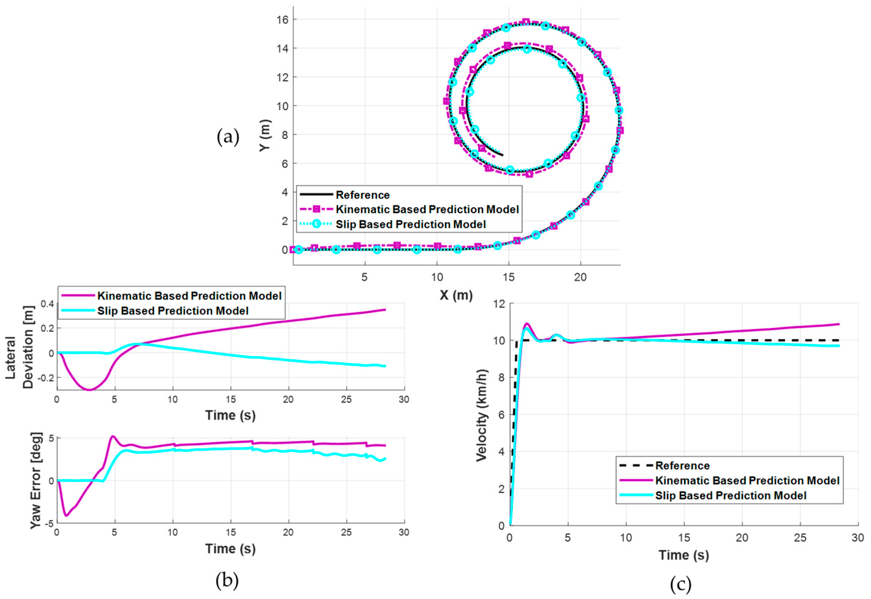
• SCENARIO 2: Steady cornering with 10 km/h velocity on a spiral.
• A further scenario is conducted for the slip-based model to emphasize its advantages and better performance:
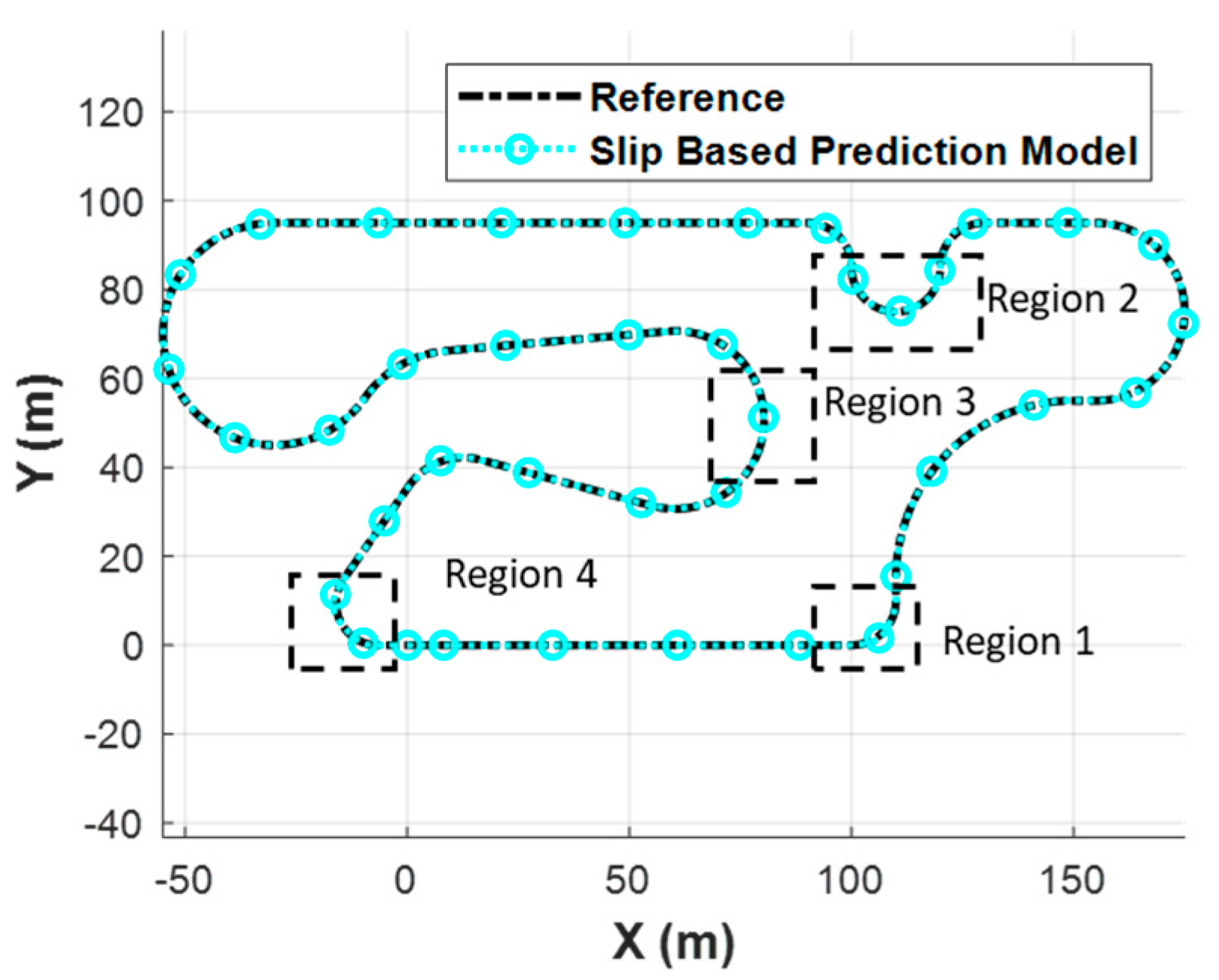
• SCENARIO 3: Trajectory tracking on a fictitious complex track at high speeds.

The selected simulation scenarios are designed to evaluate the trajectory tracking performance of the proposed controller under diverse and progressively challenging conditions. Scenario 1, inspired by the ISO 4138 automotive standard [35] for steady-state circular driving, assesses the vehicle's behavior under increasing lateral acceleration at rising speeds, effectively demonstrating the controller’s stability and precision during high-load cornering. Scenario 2 investigates low-speed handling in a progressively tightening spiral path, serving to evaluate precision at low velocities and moderate slip conditions. Finally, Scenario 3 examines controller performance over an extended trajectory with varying curvatures and higher speeds, representing a more realistic driving profile that combines transient and steady-state behaviors. Collectively, these scenarios offer a comprehensive assessment of the controller’s robustness, accuracy, and adaptability across different operational regimes.

• SCENARIO 1: R40 INCREASING SPEED

In this scenario, the vehicle drives on a R40 circle while the reference speed increases. Meanwhile, the lateral acceleration increases up to 0.5 g. This scenario is used as the benchmark for the slip-based model, where the simplification factor of $K_{Simp}$ (Equations (33) and (34)) is altered. Lateral deviation and yaw angle RMS errors with respect to the change of this factor are listed in

Table 2. Trajectory tracking errors of the slip-based model with respect to changing $K_{simp}$ simplification factor.

${\mathit{K}}_{\mathit{s}\mathit{i}\mathit{m}\mathit{p}}$	Lateral Deviation Rms [m]	Yaw Angle Error Rms [rad]
0.5	0.062	0.029
1	0.049	0.029
1.5	0.015	0.028
2	0.069	0.027
2.5	0.115	0.027
3	0.152	0.026
3.5	0.181	0.026

. Based on these results, $K_{Simp}$ = 1.5 was selected for further scenarios, since it yields the smallest lateral deviation (0.015 m RMS). Across the tested interval $K_{Simp}$ = 0.5–1.5, the RMS lateral deviation remains within the bounded range of 0.015–0.181 m, and the RMS yaw error remains within 0.026–0.029 rad. This quantifies the bounded approximation error introduced by the constant value simplification. Moreover, for $K_{Simp}$ values below 2.0, the lateral deviation error decreases, supporting the conclusion from Figure 5 that the sensitivity of $f_{exp}/V_s$ decreases with increasing speed.

In Figure 8, the results of the slip-based model are compared with the kinematic model. The kinematic-based model departs from the road at about 8.7 s (>0.5 m of lateral deviation), whereas the highest lateral deviation for the slip-based model is not higher than 0.03 m during the whole simulation (Figure 8b). At this point, the kinematic-based model reaches at most 0.17 g of lateral acceleration before 0.5 m of departure, while the slip-based model reaches up to 0.51 g of lateral acceleration at the end of the simulation.

• SCENARIO 2: 10 KMH SPIRAL

In the second scenario, the vehicle moves around a spiral trajectory with 10 km/h steady velocity, while the turning radius decreases. The slip-based vehicle is able keep the lateral deviation under 0.1 m, whereas the error of the kinematic-based model increases up to about 0.35 m (Figure 9c). Additionally, the error for the yaw angle of the vehicle reaches up to about 5 degrees for the kinematic-based model, while the slip-based model error is at most about 3.9 degrees. The lateral acceleration values reach to 0.23 g in the kinematic-based prediction model due to higher longitudinal velocity error, whereas 0.20 g is achieved in the slip-based prediction model.

In

Table 3. RMS errors of simulations with applied prediction models.

Kinematic Prediction Model	Lateral Deviation Rms [m]	Yaw Angle Error Rms [rad]	Long. Vel. Error Rms [m/s]
R20 Steady 20 km/h	0.193	0.045	0.193
Scen.1: R 40 Incr. Speed	1.343	0.070	0.407
Scen.2: 10 km/h Spiral	0.225	0.071	0.169
Slip-Based Prediction Model	Lateral Deviation Rms [m]	Yaw Angle Error Rms [rad]	Long. Vel. Error Rms [m/s]
R20 Steady 20 km/h	0.011	0.039	0.165
Scen.1: R 40 Incr. Speed	0.015	0.028	0.229
Scen.2: 10 km/h Spiral	0.057	0.054	0.115

, RMS errors for control metrics are presented, for the simulations with kinematic based prediction model and slip-based prediction model. It is obvious from the table that results of slip-based model are superior compared to results of kinematic prediction model. In the R40 case with increasing speed, the kinematic model produces significant lateral deviation errors due to departure of the vehicle from the track. Additionally, results from an extra scenario, where the vehicle negotiates an R20 corner at a steady 20 km/h, are also provided.

• SCENARIO 3: DRIVE ON A FICTITOUS COMPLEX TRACK WITH HIGH SPEED

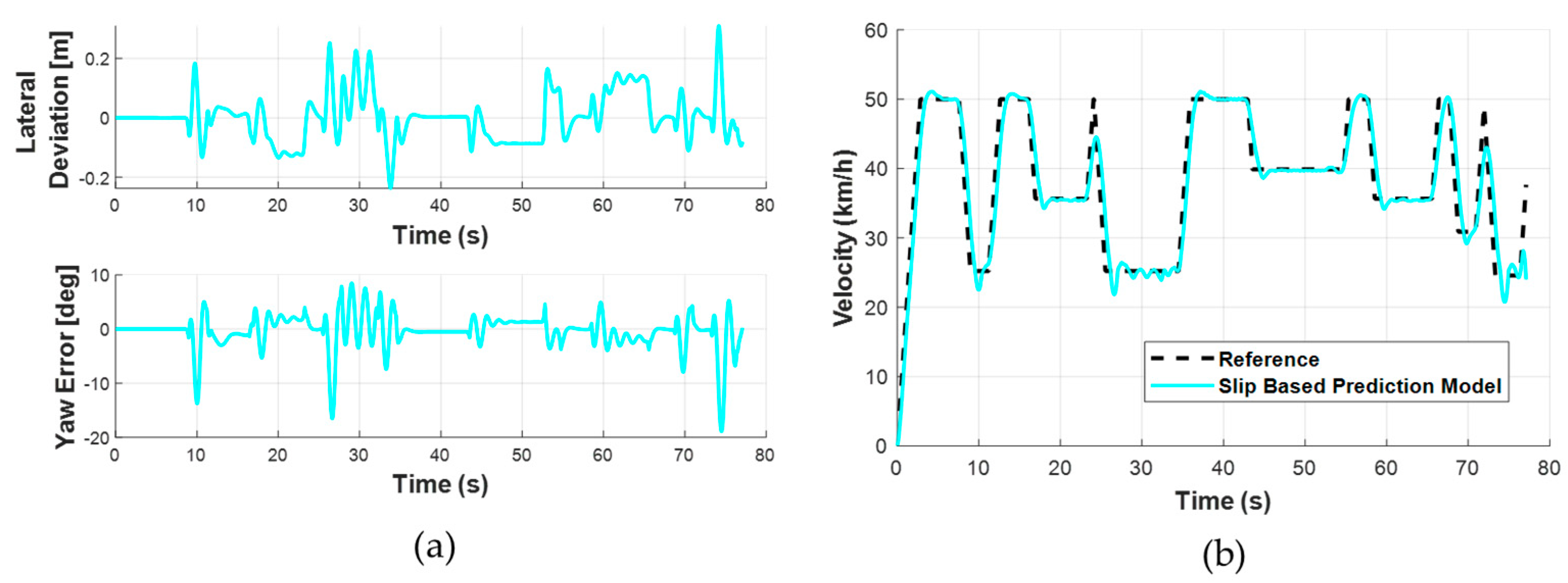
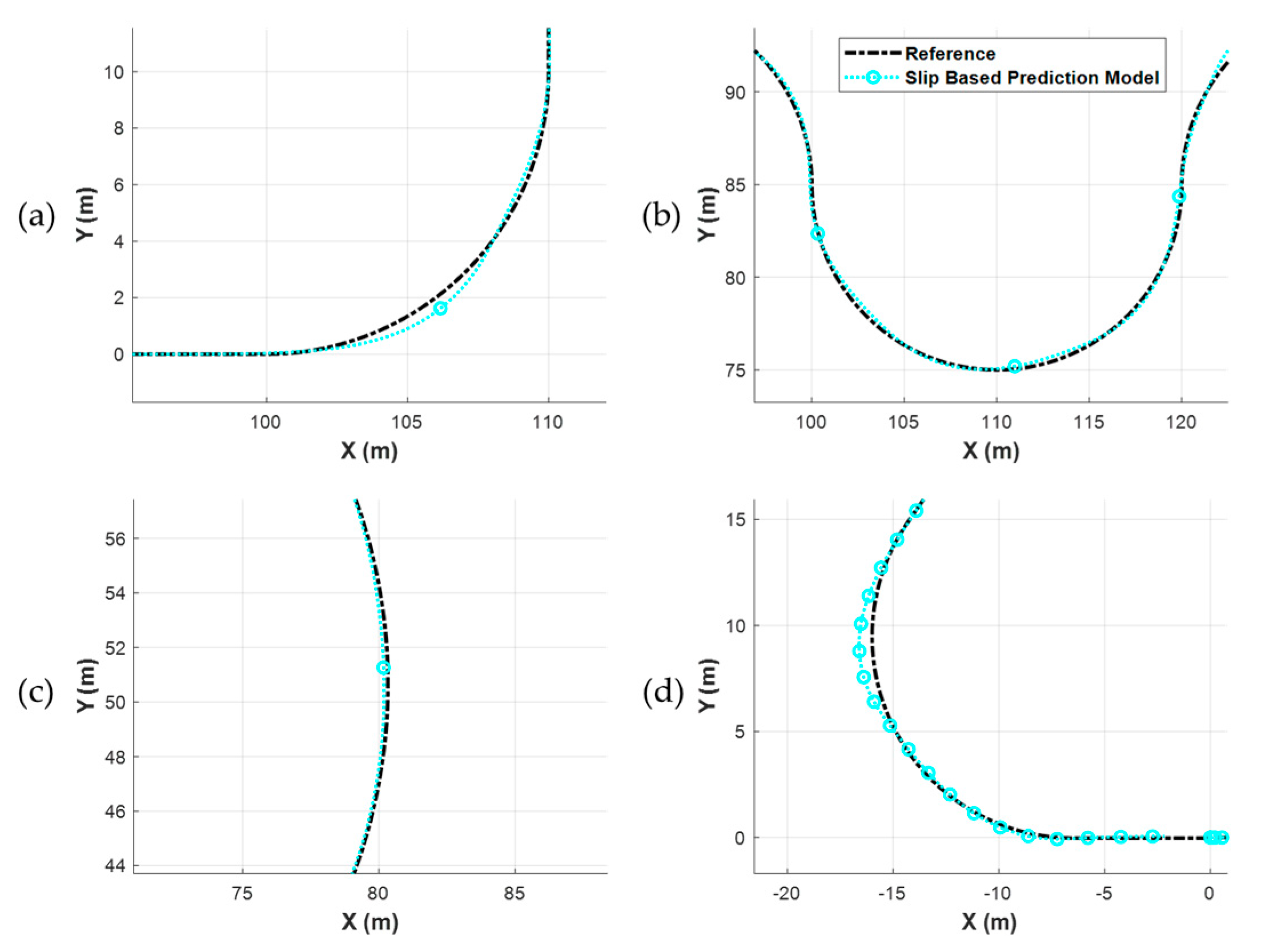
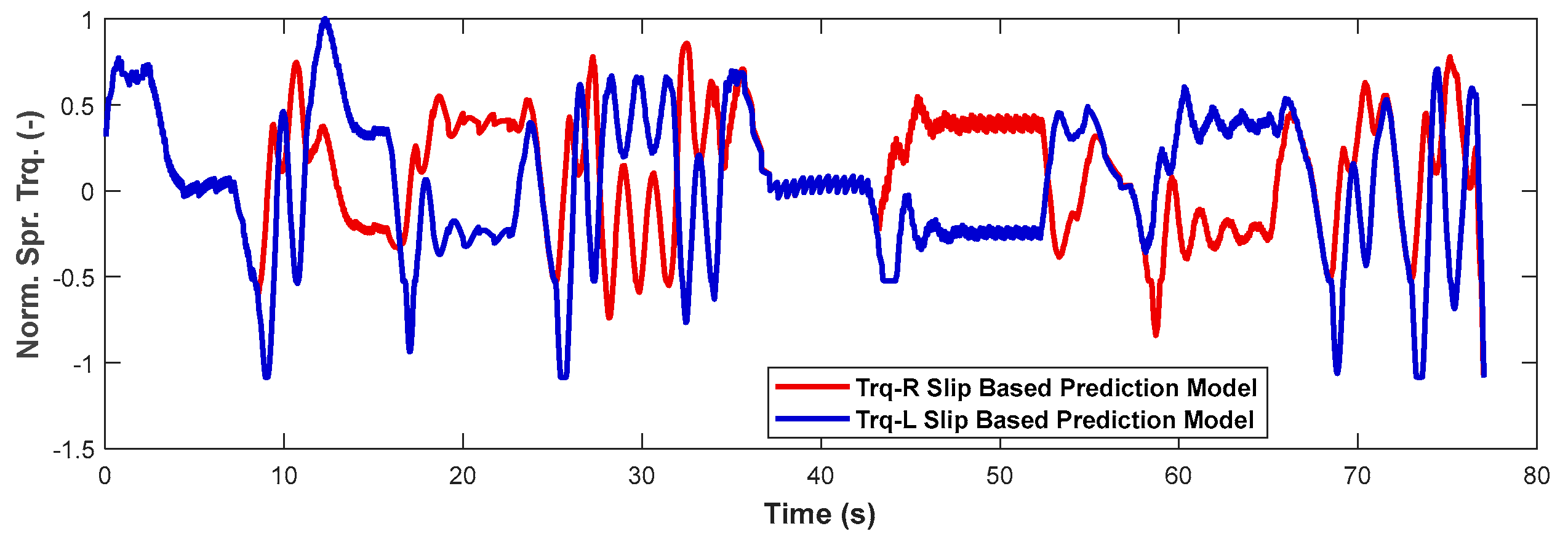
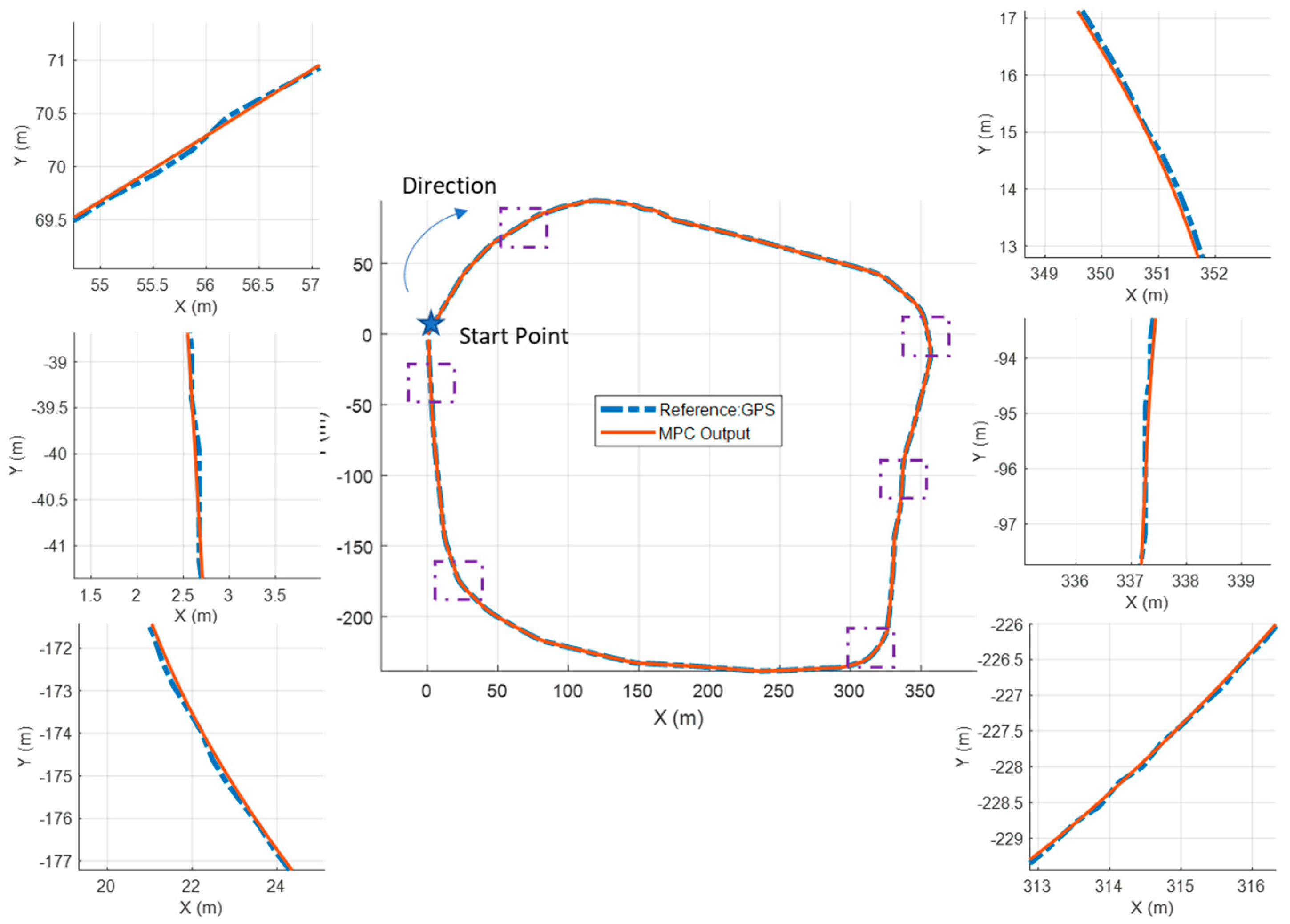
In the final scenario, free driving on a prepared complex track is analyzed (Figure 10). The reference speed profile (Figure 11b) is created up to the 50 km/h boundary. The velocity profile is limited with longitudinal and lateral acceleration of 0.5 g. According to the results, the slip based prediction model is able to control the plant well, with zoomed sections presented in Figure 12. In the results, the maximum lateral deviation is not more than 0.25 m (Figure 11a). The vehicle is also able to track the desired velocity profile with certain minimal overshoot and undershoot errors (Figure 11b). In Figure 13 outputs of the controller are presented. It can be observed from the results that the controller produces identical torque values for straight motion regions (0–8 s and 35–45 s) and for the rest of the torque values, which are distinguished with respect to the outer and inner sides of the corners. The RMS values of the lateral deviation, yaw error, and lateral velocity error values are calculated as 0.080 m, 0.057 rad, and, 0.685 m/s, respectively.

6.2. Parameter Sensitivity Analyses

In this section, the results of the parameter sensitivity analyses are presented. These analyses show the capabilities of the proposed controller, as well as the its limitations. Two different analyses are presented: (1) effect of change of friction coefficient; (2) effect of change of MPC parameters.

In first analysis, an extended version of Scenario 1 is conducted for different friction coefficient values to evaluate the controller’s capability. In this scenario, the controller maintains the trajectory of the vehicle while the reference speed is increased with 0.1 g per one second. In Figure 14a, the trajectories of each vehicle driving on the road with different friction coefficients are presented. In Figure 14b, the reference velocity profile and actual velocity profiles of these vehicle are presented. At the brake points of each maneuver, lateral acceleration values are noted. In

Table 4. Ratio of actual lateral acceleration to theoretical limit.

µ	Theoretical Limit for Lateral Acc. [g]	Reached Lateral Acc. [g]	Percentage to Limit Lateral Acc [%]
0.90	0.90	0.74	82
0.70	0.70	0.55	79
0.50	0.50	0.37	74
0.30	0.30	0.18	60
0.20	0.20	0.07	35

, the ratio of the reached lateral acceleration to the theoretical acceleration limit is presented. It can be concluded that the controller is more capable when the friction coefficient is high; however, its control limits become narrower when the friction coefficient decreases. Below the friction coefficient 0.2, the vehicle is not able to maintain the scenario. These conditions can be interpreted as the stability limit of the plant model, as well as the achievable limits of the controller.

In second analysis, changes of three crucial parameters of controller performance are analyzed: the prediction horizon (N), the control horizon (M), and the sampling time (Ts). Proper tuning of these parameters is essential to balance performance accuracy with the computational load. The results for Scenario 1, where the velocity increases on the same turning radius, are presented in

Table 5. The sensitivity analysis for MPC-specific parameters for Scenario 1.

Slip-Based Prediction Model	Sampling Time-Ts [s]	Lateral Deviation Rms [m]	Yaw Angle Error Rms [rad]	Long. Vel. Error Rms [m/s]	tavg_step [s]	tavg_step / Ts
N: 20 M: 1	0.05	0.011	0.058	0.339	0.040	79%
N: 20 M: 2		0.015	0.028	0.229	0.039	78%
N: 10 M: 1	0.05	0.068	0.017	0.123	0.022	45%
N: 10 M: 2		0.104	0.043	0.114	0.025	50%
N: 10 M: 1	0.1	0.103	0.012	0.380	0.027	27%
N: 10 M: 2		0.076	0.013	0.301	0.030	30%

. Increasing the prediction horizon N improves predictions of future behavior but also introduces additional complexity, which can increase RMS errors in certain states; for example, the yaw and longitudinal velocity errors increased when N was raised from 10 to 20. Conversely, the lateral deviation decreased over the same change of horizon. Extending the control horizon M provides the controller with more flexibility in future control actions and reduces errors, particularly in yaw and longitudinal velocity. This improvement can be observed when N = 20, as M is increased from 1 to 2. Overall, these results show that controller performance strongly depends on parameter tuning. The combination N = 20, M = 2 provides a balanced compromise between accuracy and efficiency; thus, it was used throughout this study.

Although these simulations were not deployed directly on hardware, the calculation efficiency of the controller was measured with the CPU execution time with MATLAB and compared with the defined sampling time of the controller-Ts. These calculations were carried out on a computer, with following specifications: Intel(R) Xeon(R) W-2295 CPU @ 3.00 GHz (Intel Corporation, Santa Clara, CA, USA), 64 GB DDR4 (Samsung, Suwon, Republic of Korea). In Table 5, t_{avg_step} represents the average CPU calculation time for one step for the MPC algorithm to handle the calculations. The t_{avg_step} values are compared with the sampling time in order to measure the headroom for the computation. The results show that although this computation can be handled with the given computer, real-time conditions and hardware with more limited capabilities might not sustain the operation for the configuration of N = 20 and M = 2, where the computation burden reaches ~80%. Therefore, decreasing the sampling time and prediction horizon can help in reducing the calculation burden, as can be seen in the last column of the table. This trade-off is typical for optimization-based control algorithms when considering their implementation on actual hardware.

6.3. Accuracy Analysis of the Simplified Model

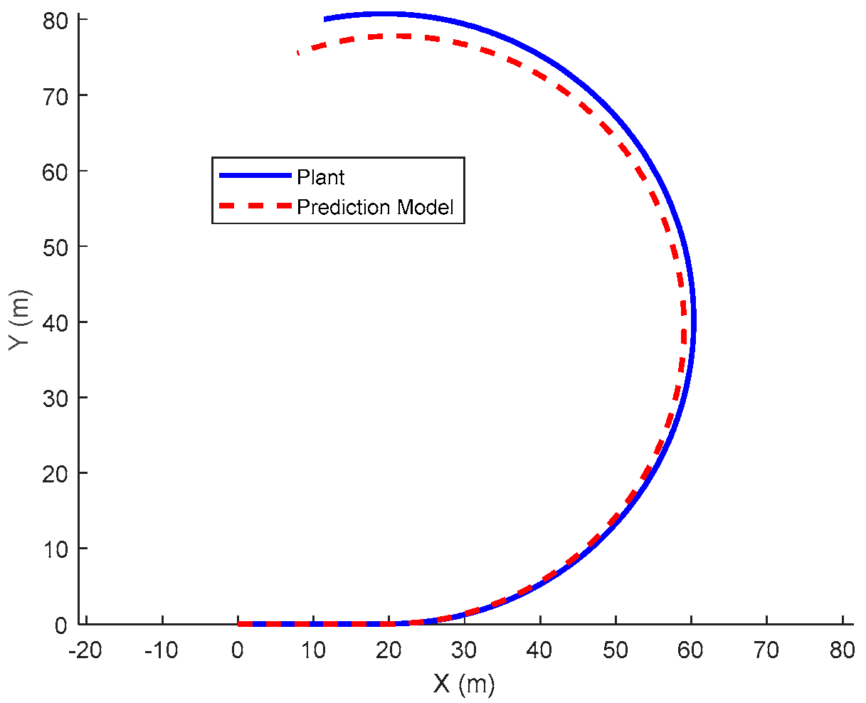
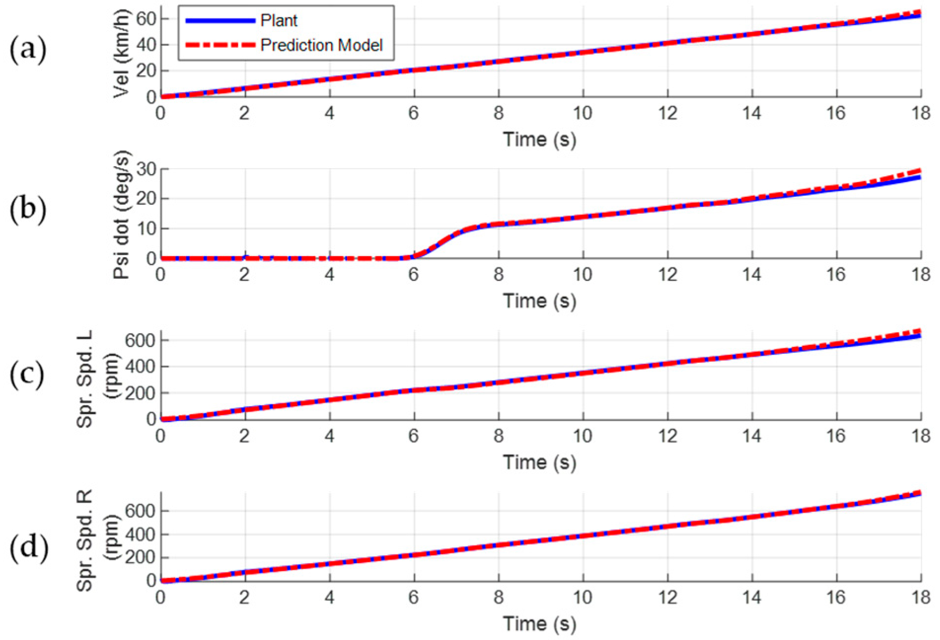
In this section, the accuracy of simplified model against the plant model and its computational efficiency are analyzed. In the accuracy analysis, Scenario 1 is applied in order to scan the lateral acceleration span, while velocity is increasing on a constant turning radius. The same torque values in Figure 15 are provided to both models and the state outputs of the models are compared. According to the results of the comparison analysis, both models follow similar trajectories, as shown in Figure 16. However, the prediction model drives on a sharper curve than the plant model. By investigating the other states of the modes, such as the velocity, yaw rate, and sprocket speed, Figure 17 presents similar trends in these states. It should be emphasized here that when the prediction model is utilized in the MPC framework, the controller uses the states of the plant as the close-loop feedback, hence output torque values are regulated accordingly. Therefore, rather than obtaining perfect matching results with the prediction model, it becomes adequate that it provides similar trends with the plant model. Therefore, it works well with the presented scenarios.

7. Test Verification for the Controller Performance

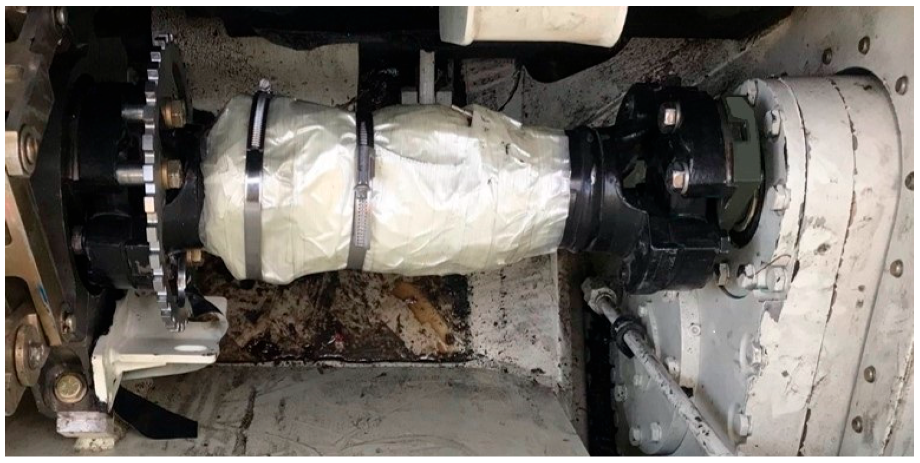
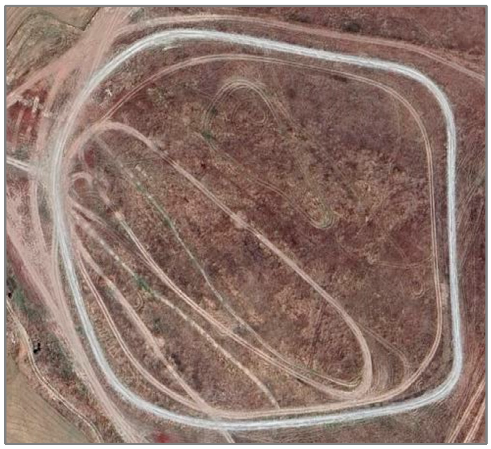
This section includes a verification of the plant model used in the study and the proposed MPC controller. Since the plant model is driven by the torque outputs of the MPC, test scenarios are focused on measurements of the vehicle trajectory and the sprocket states. Therefore, the vehicle was instrumented with different measurement devices during the tests, such as with GPS (Racelogic VBOX IISX, VBOX Automotive, Buckingham, UK), IMU (SBG Ellipse-D, SBG Systems, Carrières-sur-Seine, France), Kvaser (Kvaser AB, Mölndal, Sweden), and encoder instruments for speed measurements of the sprocket driving shafts and a strain gauge-type measurement setup for torque measurements on the sprocket driving shafts. In Figure 18 the instrumentation package for measurements on the sprocket driving shaft is presented. The asphalt test track used in the conducted experiments is demonstrated in Figure 19.

Tests were conducted in three categories: (1) low-speed cornering maneuvers on the asphalt test track; (2) touring on the asphalt with higher speeds on the test track; (3) touring on a stabilized test parkour. The main aim of these tests was to observe the performance of the vehicle at low and high speeds and use the results for a comparison with the MPC controller outputs. The obtained GPS data from the tests were converted to Cartesian coordinates and fed to the MPC controller in the simulation environment as the reference trajectory to reproduce the results of the tests.

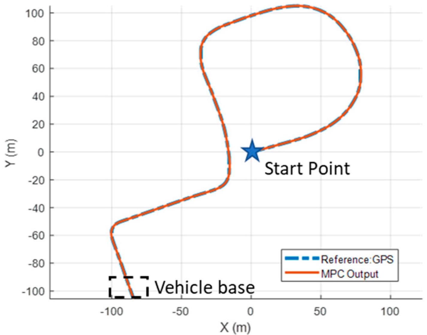
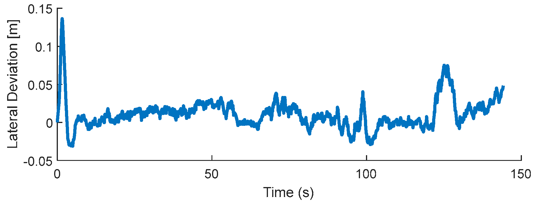
In the first scenario, the vehicle moves to its parking base at about 15 km/h of steady velocity. The GPS coordinates and results of the controlled plant model are presented in Figure 20, showing the close alignment of the test coordinates with the simulation outputs. Figure 21 verifies this fact by showing that the RMS error for the lateral deviation is 0.022 m.

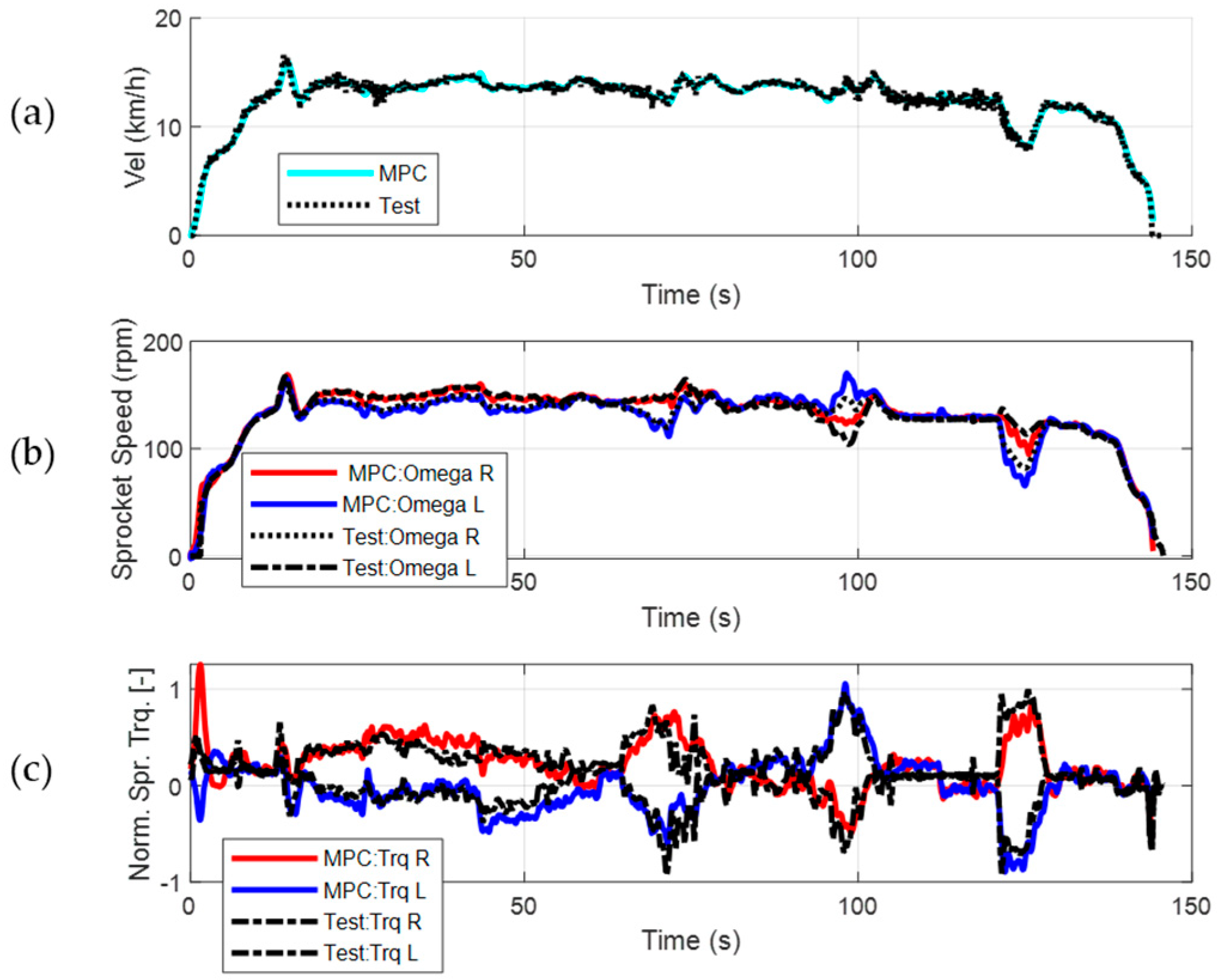
Figure 22 presents the comparison of the test data and the reproduced test in terms of the velocity profile, speed, and torques at the sprocket. The RMS differences between the reproduced simulation data and the test data for velocity, sprocket speeds, and torques are as follows: 0.3 km/h, 5.3 rpm for the right sprocket, 5.1 rpm for the left sprocket, 0.11 normalized torque for the right sprocket, and 0.12 normalized torque for the left sprocket. Normalization is conducted with respect to the absolute maximum torque value of the test data and the RMS errors correspond to 11% and 12% of this value, which are within the acceptable range, while the torque signals of the simulation results show similar trends to the measurements.

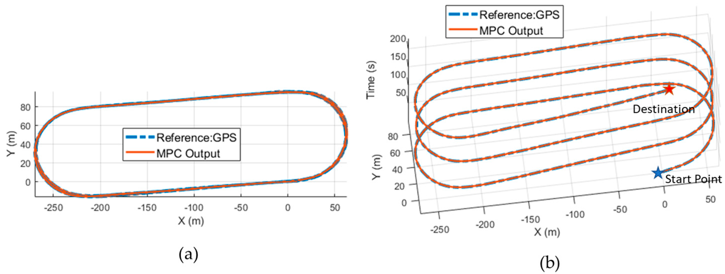
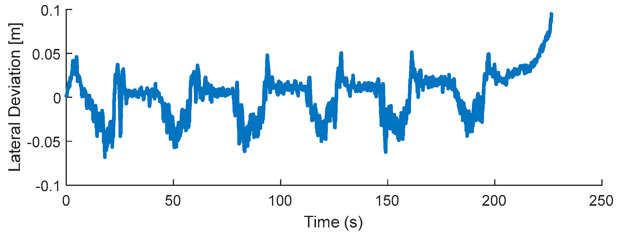
In the second scenario, the vehicle tours around the track with steady velocity of about 40 km/h. In Figure 23, the trajectories of the GPS data and reproduced test data with the MPC controller are presented. Figure 23a provides a top-down view, whereas Figure 23b illustrates the trajectory in the time domain as the third dimension, showing close alignment of test coordinates with the simulation outputs. Figure 24 verifies this fact by presenting the RMS error for the lateral deviation, which is 0.025 m.

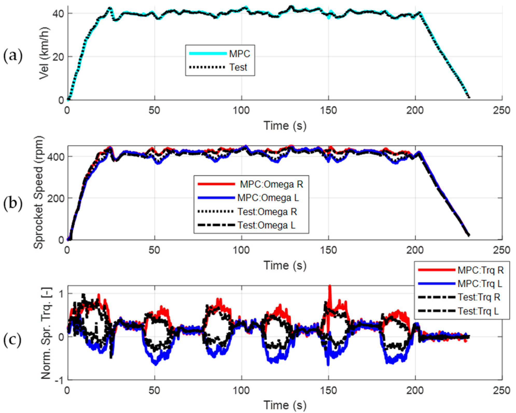
Figure 25 presents the comparison of the test data and the reproduced test in terms of velocity profiles, speeds, and torques at the sprocket. The RMS differences between reproduced simulation data and the test data for velocities, sprocket speeds, and torques are as follows: 0.4 km/h, 8.7 rpm for the right sprocket, 9.7 rpm for the left sprocket, 0.11 normalized torque for the right sprocket, and 0.18 normalized torque for the left sprocket. Normalization is conducted with respect to the absolute maximum torque value of the test data, and the RMS errors correspond to 11% and 18% of this value for the right and left sides, respectively. As a result, in both Test Scenario 1 and Test Scenario 2, the replicated simulation results show good alignment with the test results. The relatively high error in the left sprocket (inner side at corners) points out the necessity for improvement, especially at higher velocities, in future work.

Apart from the tests performed on the asphalt track, GPS data obtained from experiments conducted on a stabilized dirt road surface were also used to replicate these scenarios within the simulation environment, following the same procedure as for the asphalt track tests. These stabilized road experiments were carried out at a different time from the asphalt track trials; therefore, torque measurement sensors on the sprocket driving shafts were not available during these runs. Differing from the asphalt road, friction coefficient was applied as 0.7 to represent the loose surface of the test parkour. The mentioned parkour used in these experiments is demonstrated in Figure 26. The results of replicated simulations are presented in Figure 27 and Figure 28.

According to the results, the RMS differences between reproduced simulation data and the test data for velocities and sprocket speeds are as follows: 0.9 km/h, 13 rpm for the right sprocket and 14 rpm for the left sprocket. The RMS of the lateral deviation is about 0.028 m. These results also approve the applicability of this method in the replicated simulation environment and demonstrate that the controller delivers satisfactory performance.

Table 6. Summary table for all conducted tests for verification of trajectory tracking control (* additional tests).

Test Scen.	Test Track	Desired Steady Speed [km/h]	Average Test Velocity [km/h]	Direction / Cycle Number	Lateral Deviation Rms [m]	Long. Vel. Error Rms [km/h]
1-1	Asphalt Track	15 km/h	12.3	Test Track to Base/1	0.022	1.145
1-2 *	Asphalt Track	15 km/h	18.0	Base to Test Track/1	0.035	1.755
2-1	Asphalt Track	40 km/h	36.0	CCW/3	0.025	1.433
2-2 *	Asphalt Track	40 km/h	35.8	CW/3	0.029	1.314
3-1 *	Asphalt Track	30 km/h	29.3	CCW/3	0.024	1.113
3-2 *	Asphalt Track	30 km/h	29.7	CW/3	0.020	1.321
4-1	Stabilized Parkour	20–25 km/h	17.4	CW/1	0.028	0.919
4-2 *	Stabilized Parkour	20–25 km/h	19.0	CCW/1	0.045	2.567

summarizes the results of all previously presented tests, as well as additional trials conducted to assess the robustness of the proposed control method on firm ground. For the repeated trials, the RMS lateral deviation values on asphalt road scenarios ranged between 0.020 m and 0.035 m, with a coefficient of variation (CV) of approximately 21%. For stabilized road scenarios, the RMS lateral deviation values ranged between 0.028 m and 0.045 m, with a CV of approximately 33%, reflecting the greater variability expected under more irregular terrain conditions. The largest lateral deviation was observed in the stabilized parkour test (Scenario 4-2 in Table 6), with a value of 0.045 m. This deviation was mainly due to road surface irregularities, errors in converting GPS position data to Cartesian coordinates, and variations in the friction coefficient under stabilized road conditions, all of which make accurate replication in the simulation environment more challenging. It should be noted that the CV for stabilized road conditions was calculated from only two trials; therefore, it should be interpreted as an indicative measure rather than a statistically robust metric. Nevertheless, the measured ranges and CV values confirm the repeatability of the scenarios, the robustness of the controller in achieving its intended functionality, and the feasibility of applying it, particularly on firm ground surfaces.

8. Discussion and Conclusion

In this study, a slip-based prediction model was developed to enhance the trajectory tracking of unmanned tracked vehicles on firm road conditions by integrating it into a nonlinear model predictive control (NMPC) framework. The core novelty lies in the simplification of the exponential shear displacement formulation, yielding a bounded error but computationally efficient model of slip dynamics. The proposed approach, therefore, achieves a practical balance between accuracy and computational cost, confirming its suitability for high-speed operations in firm terrain conditions.

Comparative analyses demonstrated that the proposed slip-based controller outperformed the kinematic-based model, particularly in high-speed cornering and spiral maneuver scenarios. The slip-based model consistently maintained lateral deviation below 0.06 m RMS in comparative cases, whereas the kinematic model departed from the trajectory at increasing speeds. For a complex trajectory at up to 50 km/h, the lateral deviation remained below 0.08 m RMS, further confirming the robustness of the approach.

Sensitivity analyses were performed to assess the model’s robustness under varying conditions. The results indicated that the model maintains its high performance across different scenarios. Accuracy analyses further highlighted the model’s trend-wise similar performance against the plant model in trajectory tracking tasks. Computational efficiency evaluations indicated that with N = 20 and M = 2, the MPC used about 78% of the available sampling time, demonstrating feasibility for high-performance machines but highlighting the need for tuning in real-time embedded applications.

Validation was carried out through simulation replications using field test data from a five-wheeled tracked vehicle platform on asphalt and stabilized road conditions. The controller reproduced the vehicle’s trajectory, with lateral errors under 0.05 m RMS, and showed good agreement for sprocket speeds and torque trends, with torque estimation errors of up to 18% in asphalt test track conditions. These results confirm the effectiveness and reliability of the proposed framework for firm ground operations.

The improvements presented in this study have promising implications for real-world applications. By incorporating detailed slip dynamics into the prediction model, our approach enhances the reliability of trajectory tracking in unmanned tracked vehicles on firm ground. This advancement is crucial for applications such as unmanned heavy robotic applications and construction vehicles, where precise navigation and control are essential. The model’s ability to maintain low lateral deviations suggests its potential to improve operational efficiency and safety in these sectors.

While our model demonstrates promising results, certain limitations still require further investigation. To extend the usability of the model to more challenging environments such as uneven or deformable terrain, several factors must be addressed. The track–terrain contact mechanics will vary significantly, altering slip generation and distribution outcomes, particularly on irregular or low-cohesion surfaces. In the proposed formulation, track–terrain interaction is expressed in the shear displacement equations through the shear deformation modulus $K.$ This parameter directly influences the exponential term in the force calculation; hence, it determines the effective range of the constant factor $K_{simp}$ used in the simplified force calculations. Variations in shear deformation modulus under different terrain properties will, therefore, require either dedicated tuning of $K_{simp}$ or preferably an adaptive parameter-updating scheme to maintain the model’s accuracy. As a possible future extension, learning-based estimation techniques could be integrated with the base prediction model to identify $K_{simp}$ online, enabling the MPC to adapt in real time to changing surface conditions. Addressing these areas will bridge the gap between simulation results and practical applications.

References

1. Ly, T.T.K.; Thai, N.H.; Phong, L.T. Design of neural network-PID controller for trajectory tracking of differential drive mobile robot. Vietnam J. Sci. Technol. 2024, 62, 374–386. [Google Scholar]
2. Snider, J.M. Automatic Steering Methods for Autonomous Automobile Path Tracking. Ph.D. Thesis, Robotics Institute, Carnegie Mellon University, Pittsburgh, PA, USA, 2009. [Google Scholar]
3. Cibooglu, M.; Karapınar, U.; Söylemez, M.T. Hybrid Controller Approach for Autonomous Ground Vehicle Path Tracking Problem. In Proceedings of the 2017 25th Mediterranean Conference on Control and Automation (MED), Valletta, Malta, 3–6 July 2017. [Google Scholar]
4. Thrun, S.; Montemerlo, M.; Aron, A.; Diebel, J.; Fong, P.; Gale, J.; Stavens, D. Stanley: The robot that won the DARPA Grand Challenge. J. Field Robot. 2006, 23, 661–692. [Google Scholar] [CrossRef]
5. Hassan, N.; Saleem, A. Neural Network-Based Adaptive Controller for Trajectory Tracking of Wheeled Mobile Robots. IEEE Access 2022, 10, 13582–13597. [Google Scholar] [CrossRef]
6. SimCompanion. Available online: https://simcompanion.hexagon.com/customers/s/article/What-New-ATV-2022-3 (accessed on 3 August 2025).
7. Kong, J.; Pfeiffer, M.; Schildbach, G.; Borrelli, F. Kinematic and Dynamic Vehicle Models for Autonomous Driving Control Design. In Proceedings of the 2015 IEEE Intelligent Vehicles Symposium (IV), Seoul, Republic of Korea, 28 June–1 July 2015; pp. 1094–1099. [Google Scholar] [CrossRef]
8. Xiang, C.; Peng, H.; Wang, W.; Li, L.; An, Q.; Cheng, S. Path tracking coordinated control strategy for autonomous four in-wheel-motor independent-drive vehicles with consideration of lateral stability. Proc. Inst. Mech. Eng. Part D J. Automob. Eng. 2020, 235, 1023–1036. [Google Scholar] [CrossRef]
9. Zhang, W.; Wang, Z.; Drugge, L.; Nybacka, M. Evaluating Model Predictive Path Following and Yaw Stability Controllers for Over-Actuated Autonomous Electric Vehicles. IEEE Trans. Veh. Technol. 2020, 69, 12807–12821. [Google Scholar] [CrossRef]
10. Mahalingam, I.; Padmanabhan, C. A novel alternate multibody model for the longitudinal and ride dynamics of a tracked vehicle. Veh. Syst. Dyn. 2019, 59, 433–457. [Google Scholar] [CrossRef]
11. Ma, Z.-D.; Perkins, N.C. A Track-Wheel-Terrain Interaction Model for Dynamic Simulation of Tracked Vehicles. Veh. Syst. Dyn. 2002, 3, 401–421. [Google Scholar]
12. Wong, J.Y. Dynamics of Tracked Vehicles. Veh. Syst. Dyn. 1997, 28, 197–219. [Google Scholar] [CrossRef]
13. Çalışkan, K. Modelling and Simulation of Tracked Vehicle Dynamics. Ph.D. Thesis, Middle East Technical University, Ankara, Türkiye, 2009. [Google Scholar]
14. Zhou, L.; Wang, G.; Sun, K.; Li, X. Trajectory Tracking Study of Track Vehicles Based on Model Predictive Control. J. Mech. Eng. /Stroj. Vestnik 2019, 65, 329–342. [Google Scholar] [CrossRef]
15. Zhao, Z.; Liu, H.; Chen, H.; Xu, S.; Lang, W. Tracking Control of Unmanned Tracked Vehicle in Off-road Conditions with Large Curvature. In Proceedings of the IEEE Intelligent Transportation Systems Conference (ITSC), Auckland, New Zealand, 27–30 October 2019. [Google Scholar] [CrossRef]
16. Zhao, Z.; Liu, H.; Chen, H.; Hu, J.; Guo, H. Kinematics-aware model predictive control for autonomous high-speed tracked vehicles under the off-road conditions. Mech. Syst. Signal Process. 2019, 123, 333–350. [Google Scholar] [CrossRef]
17. Tao, J.; Liu, H.; Li, Y.; Guan, H.; Liu, J.; Chen, H. Design of Trajectory Tracking Controller of Unmanned Tracked Vehicles Based on Torque Control. In Proceedings of the IEEE International Conference on Unmanned Systems (ICUS), Beijing, China, 15–17 October 2021. [Google Scholar] [CrossRef]
18. Maclaurin, B. A skid steering model using the Magic Formula. J. Terramech. 2011, 48, 247–263. [Google Scholar] [CrossRef]
19. Liang, J.; Tian, Q.; Feng, J.; Pi, D.; Yin, G. A Polytopic Model-Based Robust Predictive Control Scheme for Path Tracking of Autonomous Vehicles. IEEE Trans. Intell. Veh. 2024, 9, 3928–3939. [Google Scholar] [CrossRef]
20. Liang, J.; Lu, Y.; Wang, F.; Feng, J.; Pi, D.; Yin, G.; Li, Y. ETS-Based Human–Machine Robust Shared Control Design Considering the Network Delays. IEEE Trans. Autom. Sci. Eng. 2024, 22, 17501–17511. [Google Scholar] [CrossRef]
21. Li, B.; Pan, Z.; Liu, J.; Zhou, S.; Liu, S.; Chen, S.; Wang, R. Integrated Control of a Wheel–Track Hybrid Vehicle Based on Adaptive Model Predictive Control. Machines 2024, 12, 485. [Google Scholar] [CrossRef]
22. Zhan, J.; Li, W.; Wang, J.; Xiong, S.; Wu, X.; Shi, W. Research on Trajectory Planning and Tracking Algorithm of Crawler Paver. Machines 2024, 12, 650. [Google Scholar] [CrossRef]
23. Inal, T.T.; Cansever, G.; Yalçın, B.; Çetin, G.; Hartavi, A.E. Enhanced Energy Efficiency through Path Planning for Off-Road Missions of Unmanned Tracked Electric Vehicle. Vehicles 2024, 6, 1027–1050. [Google Scholar] [CrossRef]
24. Strawa, N.; Ignatyev, D.I.; Zolotas, A.C.; Tsourdos, A. On-Line Learning and Updating Unmanned Tracked Vehicle Dynamics. Electronics 2021, 10, 187. [Google Scholar] [CrossRef]
25. Fan, J.; Yan, P.; Li, R.; Liu, Y.; Wang, F.; Liu, Y.; Chen, C. Decoupled Adaptive Motion Control for Unmanned Tracked Vehicles in the Leader-Following Task. World Electr. Veh. J. 2024, 15, 239. [Google Scholar] [CrossRef]
26. Zhang, R.; Zhou, W.; Liu, H.; Gong, J.; Chen, H.; Khajepour, A. Similarities between Wheels and Tracks: A “Tire Model” for Tracked Vehicles. IEEE Trans. Veh. Technol. 2024, 73, 16416–16431. [Google Scholar] [CrossRef]
27. Ozdemir, M.N.; Unlusoy, Y.S. Steering Dynamics of Tracked Vehicles. Master’s Thesis, Middle East Technical University, Ankara, Türkiye, 2016. [Google Scholar]
28. Garber, M.; Wong, J.Y. Prediction of ground pressure distribution under tracked vehicles—I. An analytical method for predicting ground pressure distribution. J. Terramech. 1981, 18, 1–23. [Google Scholar] [CrossRef]
29. Weiss, K.R. Skid Steering. Proc. Inst. Mech. Eng. Part D J. Automob. Eng. 1971, 22–25. [Google Scholar]
30. Kitano, M.; Jyozaki, H. A theoretical analysis of steerability of tracked vehicles. J. Terramech. 1976, 13, 241–258. [Google Scholar] [CrossRef]
31. Wong, J.Y.; Chiang, C.-F. A general theory for skid steering of tracked vehicles on firm ground. Proc. Inst. Mech. Eng. Part D J. Automob. Eng. 2001, 215, 343–355. [Google Scholar] [CrossRef]
32. Chiang, C.-F. Handling Characteristics of Tracked Vehicles on Non-Deformable Surfaces. Master’s Thesis, Ottawa-Carleton Institute for Mechanical and Aerospace Engineering, Department of Mechanical and Aerospace Engineering, Ottawa, ON, Canada, June 1999. [Google Scholar]
33. Ehlert, W.; Hug, B.; Schmid, I.C. Field measurements and analytical models as a basis of test stand simulation of the turning resistance of tracked vehicles. J. Terramech. 1992, 29, 57–69. [Google Scholar] [CrossRef]
34. Zou, Y.; Sun, F.; Hu, X.; Guzzella, L.; Peng, H. Combined optimal sizing and control for a hybrid tracked vehicle. Energies 2012, 5, 4697–4710. [Google Scholar] [CrossRef]
35. ISO 4138:2021; Passenger Cars—Steady-State Circular Driving Behaviour—Open-Loop Test Methods. International Organization for Standardization: Geneva, Switzerland, 2021.
36. Çiloglu, Ç.; Kutluay, E. Performance Improvement of Pure Pursuit Algorithm via Online Slip Estimation for Off-Road Tracked Vehicle. Sensors 2025, 25, 4242. [Google Scholar] [CrossRef] [PubMed]
Figure 2. (a) Simple kinematic model (b) and sliding kinematic model.
Machines 13 00817 g002
Figure 3. Shear displacement-based plant model [27]: (a) kinematics of the model; (b) kinematics of the discretized track pads.
Machines 13 00817 g003
Figure 4. Comparison of sprocket torques at different theoretical turning radii in logarithmic scale based on the test data [33] and results produced with the general theory [31] and plant model [27]: (a) Results for 7.5 km/h; (b) Results for 14.2 km/h; (c) Results for 21.3 km/h; (d) Results for 29 km/h.
Machines 13 00817 g004
Figure 5. Change of K s i m p = f e x p / V s function with respect to changes of V s and V t for the mid road wheel.
Machines 13 00817 g005
Figure 6. Layout of the proposed prediction model.
Machines 13 00817 g006
Figure 7. Flowchart of MPC framework.
Machines 13 00817 g007
Figure 8. Scenario 1 (R40: increasing speed): (a) trajectory results; (b) tracking errors; (c) longitudinal velocity tracking results.
Machines 13 00817 g008
Figure 9. Scenario 2 (10 km/h spiral motion): (a) trajectory results; (b) tracking errors; (c) longitudinal velocity tracking results.
Machines 13 00817 g009
Figure 10. Scenario 3: Fictitious complex drive track.
Machines 13 00817 g010
Figure 11. Results of Scenario 3: (a) tracking errors; (b) longitudinal velocity tracking results.
Machines 13 00817 g011
Figure 12. Trajectory following results of Scenario 3: (a) zoom region 1; (b) zoom region 2; (c) zoom region 3; (d) zoom region 4.
Machines 13 00817 g012
Figure 13. Normalized torque outputs of MPC controller for Scenario 3.
Machines 13 00817 g013
Figure 14. Parameter sensitivity friction coefficient: (a) trajectories of vehicles for different friction coefficient values; (b) velocity profiles for different friction coefficient values.
Machines 13 00817 g014
Figure 15. Torque input for model comparison.
Machines 13 00817 g015
Figure 16. Trajectory outputs of the plant model and prediction model for Scenario 1.
Machines 13 00817 g016
Figure 17. Comparison of state outputs of the plant model and prediction model for Scenario 1: (a) velocity; (b) yaw rate; (c) speed of left sprocket; (d) speed of right sprocket.
Machines 13 00817 g017
Figure 18. Instrumentation on the sprocket driving shaft for measurements of shaft speed and torque.
Machines 13 00817 g018
Figure 19. Top view of the asphalt test track (due to sensitive information, the test track view is cropped).
Machines 13 00817 g019
Figure 20. Results of Test Scenario 1: GPS coordinates vs. reproduced MPC results.
Machines 13 00817 g020
Figure 21. Results of Test Scenario 1—lateral deviation.
Machines 13 00817 g021
Figure 22. Results of Test Scenario 1—comparison of test vs. reproduced data: (a) velocity profile; (b) sprocket speeds; (c) normalized sprocket torque.
Machines 13 00817 g022
Figure 23. Results of Test Scenario 2: GPS coordinates vs. reproduced MPC results: (a) top view; (b) trajectory change with respect to time.
Machines 13 00817 g023
Figure 24. Results of Test Scenario 2—lateral deviation.
Machines 13 00817 g024
Figure 25. Results of Test Scenario 2—comparison of test vs. reproduced data: (a) velocity profile; (b) sprocket speeds; (c) normalized sprocket torque.
Machines 13 00817 g025
Figure 26. Top view of the stabilized test parkour [36].
Machines 13 00817 g026
Figure 27. Results of test scenario on stabilized roads: GPS coordinates vs. reproduced MPC results.
Machines 13 00817 g027
Figure 28. Results of test scenario on stabilized parkour: (a) velocity profile comparison; (b) sprocket speed comparison; (c) lateral deviation.
Machines 13 00817 g028