A Novel Transfer Kernel Enabled Kernel Extreme Learning Machine Model for Cross-Domain Condition Monitoring and Fault Diagnosis of Bearings

Abstract

Kernel transfer learning (KTL), as a kind of statistical transfer learning (STL), has provided significant solutions for cross-domain condition monitoring and fault diagnosis of bearings due to its ability to capture relationships and reduce the gap between source and target domains. However, most conventional kernel transfer methods only set a weighting parameter ranging from 0 to 1 for those functions measuring cross-domain differences, while the intra-domain differences are ignored, which fails to completely characterize the distributional differences to some extent. To overcome these challenges, a novel transfer kernel enabled kernel extreme learning machine (TK-KELM) model is proposed. For model pre-training, a parallel structure is designed to represent the state and change of vibration signals more comprehensively. Subsequently, intra-domain correlation is introduced into the kernel function, which aims to release the weight parameters that describe the inter-domain correlation and break the range limit of 0–1. Consequently, intra-domain as well as inter-domain correlations can boost the authenticity of the transfer kernel jointly. Furthermore, a similarity-guided feature-directed transfer kernel optimization strategy (SFTKOS) is proposed to refine model parameters by calculating domain similarity across different feature scales. Subsequently, the kernels extracted from different scales are fused as the core functions of TK-KELM. In addition, an integration framework via function principal component analysis with maximum mean difference (FPCA-MMD) is designed to extract the multi-scale domain-invariant degradation indicator for boosting the performance of TK-KELM. Finally, related experiments verify the effectiveness and superiority of the proposed TK-KELM model, improving the accuracy of condition monitoring and fault diagnosis.

1. Introduction

Bearings, as critical components within real-world mechanical systems, play a vital role in the reliability and functionality of machinery [1]. Consequently, bearing condition monitoring (BCM) and bearing fault diagnosis (BFD) are essential for preventing unexpected breakdowns and ensuring operational efficiency. Recently, data-driven methods for BCM and BFD have attracted significant attention due to their capability to effectively identify the health state of equipment. They mainly consist of algorithms based on machine learning and methods based on signal processing. Among these methods, machine learning (ML) [2] algorithms have emerged as a powerful tool, establishing mapping models between measured sensor data and the operational states of machinery, ultimately enabling accurate health state diagnosis [3]. Machine learning encompasses a variety of algorithms such as K-nearest neighbors [4], Bayesian learning [5], deep learning [6] and meta-learning [7] that can be employed to analyze sensor data and predict fault conditions. Different from the machine learning algorithms, signal processing-based methods depend on domain-specific prior knowledge to guide feature extraction. For instance, Antoni [8] provided quantifiable measures to characterize signal deviations from healthy states, enabling the early detection of incipient faults through systematic feature quantification. The blind deconvolution techniques proposed by Chen et al. [9] effectively suppress background noise and enhance fault-related impulses. Additionally, Chen et al. [10] also developed a signal decomposition method combined with cyclic spectral correlation, making it particularly effective for diagnosing faults under varying operating conditions. These signal processing methods complement data-driven machine learning approaches, forming a comprehensive toolkit for addressing the challenges in real-world condition monitoring and fault diagnosis scenarios. However, most data-driven algorithms rely on sufficient datasets, and insufficient samples can hinder the effective training of ML models and severely limit their effectiveness [11]. In addition, machines often operate under varying conditions in real-world scenarios, which will cause data distribution differences between training and testing data.

Technically, these aforementioned challenges can be settled by cross-domain learning approaches, such as statistical transfer learning (STL), joint learning, adversarial task augmentation and so on [12]. Among them, STL provides a promising solution to address challenges due to its simplicity and efficiency [13]. Technically, STL belongs to transfer learning (TL), which can acquire knowledge from other relevant fields to solve the drawbacks of traditional ML-based models. The particularity of STL lies in that it focuses on leveraging source-domain specific statistical knowledge to boost the performance of target tasks under the framework of statistical modelling. Theoretically benefitting from the abilities of parameter learning from statistical models as well as knowledge transfer from transfer learning, STL can extract the relatively more global transferable knowledge [14], thereby enabling excellent knowledge transfer capabilities and better generalization for BCM and BFD under changing operating conditions.

Recently, this method has attracted the attention of many scholars. For example, Hu et al. [15] developed a transfer learning strategy based on balanced adaptation regularization for unsupervised BFD across domains. Ganin et al. [16] introduced a novel domain adaptation framework that utilizes adversarial training to minimize the inter-domain distribution gap. Ganin et al. [17] introduced a novel adversarial domain classifier to optimize both classification tasks and domain adaptation. However, the nonlinearity of vibration data would increase the complexity of the model-training process to some extent.

In light of this, kernel transfer learning (KTL), as a kind of STL approach, has emerged as a particularly effective method. KTL utilizes kernel functions to project data onto elevated-dimensional feature spaces, allowing for a more nuanced comprehension of the data’s fundamental patterns [18]. Additionally, by leveraging the kernel trick and sparse representations, KTL can also address the computational challenges arising from nonlinear data. Theoretically, KTL expands the application scope of STL techniques for more complex scenarios. For KTL, plenty of strategies have emerged in recent years, including the following two major aspects: (1) Optimization and selection of kernel function. For example, Cao et al. [19] applied a single parameter to represent the relationship between the two domains in a standard transfer learning scenario involving two domains. Wagle et al. [20] further extended this approach by differentiating between the covariance of the two domains. Wei et al. [21] generalized a transfer kernel to solve a multi-source-domain task through setting up the similarity coefficient of each pair of source-target domains. (2) Optimization of domain alignment. For example, Wei et al. [22] developed a multi-kernel learning approach that integrates multiple kernel functions to facilitate parallel processing capabilities. Zheng et al. [23] proposed a Gaussian process regression of the adaptive two-stage model using the matching kernel. Lu et al. [24] utilized sample correlation and learnable kernels to realize domain adaptive learning. Wu et al. [25] applied an adaptive deep transfer learning method for domain adaptive learning. Additionally, recent advancements in zero-faulty or limited-fault data scenarios deserve further attention. For example, emerging techniques like the shrinkage mamba relation network (SMRN) [26] leverage out-of-distribution data augmentation to enable fault detection and localization in rotating machinery under zero-faulty data regimes. Such methods address the challenge of absent fault labels by generating synthetic anomalies, bridging gaps in data scarcity. However, most existing studies only consider and quantify inter-domain differences by adopting a single parameter ranging from 0 to 1 for kernel optimization. This limits the model’s ability to capture the global distributional differences to some extent.

In order to tackle the aforementioned questions, this article proposes a novel transfer kernel enabled kernel extreme learning machine (TK-KELM) model for BCM and BFD. Firstly, a parallel structure for the pre-training of the model is designed to more fully represent the state and change of vibration signals. Then, the intra-domain differences are involved into the optimization process, thereby releasing the weight parameters that describe the inter-domain relationships and enabling them to break the limitations of the original range from 0 to 1. Subsequently, those transfer kernels undergo optimization through a similarity-guided feature-directed transfer kernel optimization strategy (SFTKOS), which fine-tunes model parameters based on domain similarities across different feature scales. Additionally, an integrated framework that combines functional principal component analysis with maximum mean difference (FPCA-MMD) is introduced to derive multi-scale domain-invariant degradation indicators for enhancing the model’s overall robustness. Finally, the gradient iterative segmentation (GIP) algorithm and support vector machine (SVM) are applied for BCM and BFD, respectively, demonstrating the effectiveness of this methodology. The key contributions of this study are outlined as follows:

• A new mechanism for KTL is proposed to capture both intra-domain and inter-domain differences, which breaks the limitation of the original parameter ranging scope (from 0 to 1) in a conventional KTL framework, and shows strong adaptability for cross-domain transfer learning.
• A similarity-guided feature-directed transfer kernel optimization strategy is designed under the framework of parallel structure and MMD to optimize kernel parameters, which is beneficial for mining domain invariant features completely and improving the cross-domain learning performance.
• A novel transfer kernel enabled kernel extreme learning machine (TK-KELM) model is proposed, which is beneficial for boosting the adaptability of the model for BCM and BFD.

The organization of this article is outlined below. Section 2 delves into the related knowledge essential for understanding our work. Section 3 introduces the proposed method, detailing its components and the theoretical underpinnings. Section 4 presents two case studies to illustrate the practical application and efficacy of the approach proposed in this paper. In conclusion, Section 5 wraps up the article.

2. Related Knowledge

2.1. Statistical Transfer Learning

Statistical transfer learning (STL) provides a distinct perspective on transfer learning by approaching it from a statistical viewpoint. STL can be described as follows [23]: given a source domain $D_S$ with the assignment task $T_S$ and a target domain $D_T$ with the assignment task $T_T$, STL aims to learn domain-invariant statistical knowledge between domains and boost the performance of target $T_T$. Specifically, the target domain $D_T$ comprises a sample set $X_T$ containing monitored data from the target object, which follows a data distribution $P\left(x_T\right)$, that is, $D_T=\left\{X_T,P\left(x_T\right)\right\}$. Source domain $D_S$ contains the sample set $X_S$ of relevant bearing data and its corresponding distribution $P\left(x_S\right)$, that is, $D_S=\left\{X_S,P\left(x_S\right)\right\}$. In this study, let $N_T$ (the sample quantity of $D_T$) $\ll N_S$(the sample quantity of $D_S$), which means the target domain has limited data, while adequate data from another working condition (namely source domain $D_S$) are available. From a statistical standpoint, data from different conditions are analyzed based on their distinct marginal distributions [27]. Whereas, due to the complexity brought on by varying measurement environments and operational conditions, the data gathered in another working condition naturally exhibits differences in their marginal probability distributions. For a robust cross-domain BCM and BFD model, STL begins by building specific statistical models designed for each unique task or domain, such as linear regression frameworks and Gaussian process methodologies. Subsequently, various statistical methods, including Bayesian inference and boosting techniques, are employed to enable the effective transfer of domain-invariant statistical knowledge between these models, enhancing the overall learning process across different domains.

However, with the increase in data complexity, traditional STL methods will encounter challenges in dealing with highly nonlinear data distributions. In contrast, KTL provides a powerful tool to deal with this problem. KTL tries to map both domains to the regenerated kernel Hilbert space for weakening the distributional gap of different domains. The core idea of KTL is to define an implicit nonlinear mapping $\varphi \left(x\right)$ through the kernel function $k\left(x,x^{\prime }\right)$, which transfers the input data from the initial space to the Hilbert space. Then, maximum mean discrepancy (MMD) [27] is adopted to measure the distributional difference, which can be expressed as follows:

$$MM{D}^2\left(D_S,D_T\right)={‖{\displaystyle \frac{1}{n_s}}{\displaystyle \sum _{i=1}^{n_s}\varphi \left(x_{si}\right)-}{\displaystyle \frac{1}{n_t}}{\displaystyle \sum _{i=1}^{n_t}\varphi \left(x_{ti}\right)}‖}_{\mathrm{H}}^2$$

(1)

where $\varphi \left(x\right)$ is the data implicitly mapped by the kernel function, $\mathrm{H}$ represents regenerated kernel Hilbert space and $x_{si}$ and $x_{ti}$ are the data of both domains, respectively. By minimizing MMD, the distributional alignment between domains can be optimized in the regenerated kernel Hilbert space. Finally, the mapped $D_S$ can be regarded as an auxiliary dataset to boost the performance of $T_T$.

2.2. KELM Model

The basic structure of KELM is made up of a single-layer feedforward architecture, which includes an input layer, a hidden layer and an output layer.

(1) The input layer: The input samples are recorded as $\mathit{x}=\left[x_1,x_2,\dots ,x_n\right]$, where $n$ is the quantity of samples, corresponding to the neurons in the input layer.

(2) The hidden layer: Given a KELM model with $m$ hidden units, the output matrix of the hidden layer can be denoted as follows:

$${\mathit{H}}_m=\left(\begin{array}{ccc}{h}_1\left(x_1\right)& \dots & h_1\left(x_1\right)\\ ⋮& \ddots & ⋮\\ h_m\left(x_n\right)& \dots & h_m\left(x_n\right)\end{array}\right)$$

(2)

where $h_m\left(x\right)$ refers to the feature mapping function. The columns of ${\mathit{H}}_m$ represent the output of the m-th hidden layer neuron for all samples. The parameters of the hidden layer are initialized randomly. The input is mapped to the hidden layer space through the feature mapping process, followed by the activation function below:

$$h_m\left(x\right)=a\left(w_{m_0}+w_{m_1}{x}_{m_1}+\dots +w_{m_n}{x}_{m_n}\right)$$

(3)

where $w_m$ represents the connection weight vector from the hidden layer to the output layer.

(3) The output layer: Then, the output can be formulated as follows:

$$f_m\left(x\right)={\displaystyle \sum _{k=1}^m{\beta }_k{h}_k\left(x\right)}$$

(4)

where ${\beta }_k$ represents the vector which connects the hidden layer nodes to the output neurons. Supposing that the vector of the timing signal is represented as $T={\left(t_1,t_2,\dots ,t_n\right)}^T$, according to the literature [28], $\beta$ can be expressed as follows:

$$\beta ={\left({\displaystyle \frac{I}{C}}+\mathit{H}{\mathit{H}}^T\right)}^{-1}{\mathit{H}}^{T}T$$

(5)

where $I$ stands for the unit matrix of appropriate dimensions, $C$ represents a regularization parameter and $H$ is the stack matrix output by all hidden layers. Therefore, the output becomes the following:

$$f_L\left(x\right)=h\left(x\right){\left({\displaystyle \frac{1}{C}}+\mathit{H}{\mathit{H}}^T\right)}^{-1}{\mathit{H}}^{T}T$$

(6)

Selecting the core function $\mathit{K}\left(x_i,x_j\right)$ and its expression can also be expressed as follows:

$$K\left(x_i,x_j\right)=h_m(x_i)h_m\left(x_j\right),\begin{array}{cc} & \mathit{K}=\mathit{H}{\mathit{H}}^T\end{array}$$

(7)

With this modification, the output becomes the following:

$$f\left(x\right)=h\left(x\right){\mathit{H}}^T{\left(\mathit{K}+{\displaystyle \frac{1}{C}}\right)}^{-1}T$$

(8)

3. Proposed Method

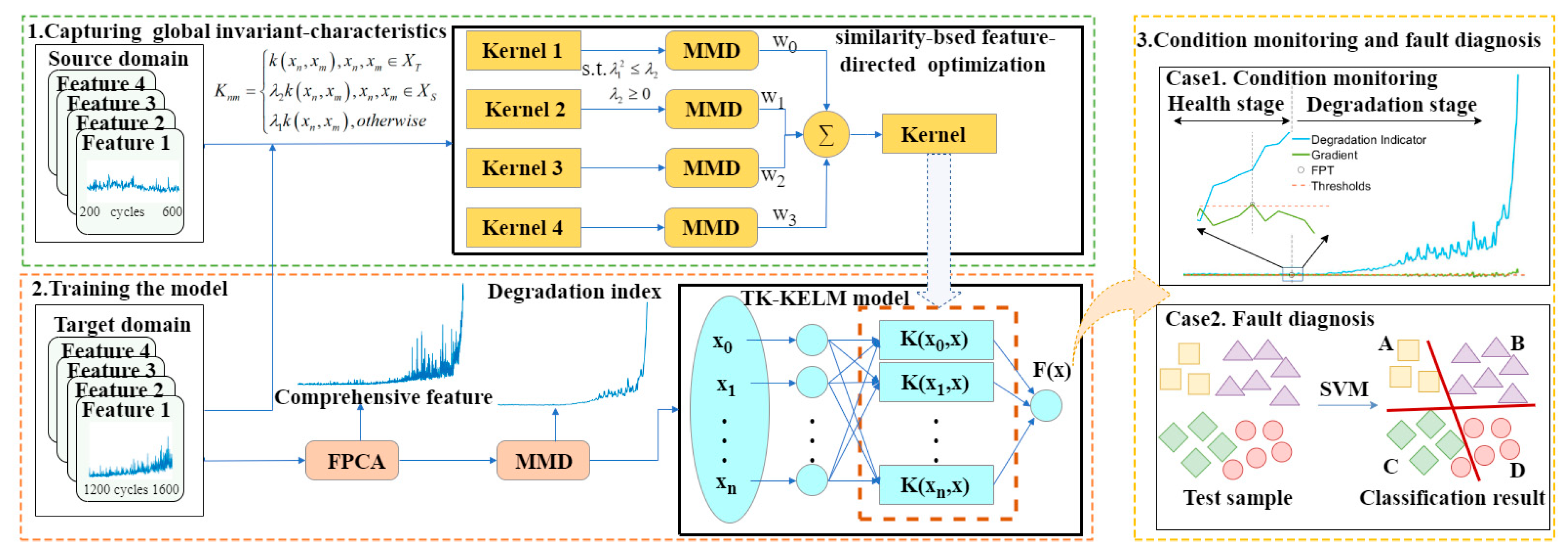
As presented in Figure 1, the overall block diagram of the proposed methodology is shown. The proposed method mainly includes three parts: (1) capturing global invariant-characteristics, (2) training the model and (3) condition monitoring and fault diagnosis. Firstly, diverse sets of time-domain characteristics are retrieved from the source domain, and the domain correlation is captured through employing the kernel function, and then the parameters are optimized through SFTKOS. Secondly, the FPCA-MMD method is utilized to construct the bearing degradation index for model training and prediction. Finally, given optimized transfer kernels as well as domain-invariant indexes, BCM and BFD are realized by solving the problem of distribution differences caused by variable working conditions.

3.1. Capturing Global Invariant-Characteristics

In STL, one of the challenges is quantifying the relationship of inter-domain data sets, particularly when the $D_T$ has limited annotated data. This paper combines feature transfer and Bayesian methods to address this issue. First, the parameters $K_1$, $K_2$, $K_3$ are defined as the covariance matrices of $D_S$ with $D_S$, $D_S$ with $D_T$ and $D_T$ with $D_T$, respectively. The parameter $K_{ST} = {\lambda }_1{K}_2$ is then designed to represent the similarity between $D_S$ and $D_T$. For the feature transfer method, the characteristics matrix of the target domain will be $X_T^{\prime } = {\lambda }_1{K}_2^T{K}_1^{-1}{X}_S$, where ${\lambda }_1$ is in range ${\lambda }_1\in \left(0,+\infty \right)$. However, in the Bayesian approach, the relation between $D_S$ and $D_T$ is viewed probabilistically. In this case, ${\lambda }_1$ is bounded within $\left[0,1\right]$, representing the chance associated with this relationship. Consequently, ${\lambda }_1$ should become a free parameter rather than a fixed probability distribution.

According to the literature [24], it is assumed that the prior knowledge probability for different similarities is uniform, which allows ${\lambda }_1$ to remain free while still providing a probabilistic interpretation. An additional parameter, $K_{SS}={\lambda }_2{K}_1$, is introduced to refine the posterior understanding of the source $D_S$ and $D_T$, thus further relaxing constraints on the parameter ${\lambda }_1$.

As a result, the proposed transfer kernel can be expressed as follows:

$${\mathit{K}}_{nm}=\left\{\begin{array}{l}k\left(x_n,x_m\right),x_n,x_m\in X^T\\ {\lambda }_{2}k\left(x_n,x_m\right),x_n,x_m\in X^S\\ {\lambda }_{1}k\left(x_n,x_m\right),otherwise\end{array}\right.$$

(9)

where ${\lambda }_1^2\le {\lambda }_2$, ${\lambda }_2\ge 0$ and $k\left(·\right)$ represents the well-known radial basis function (RBF) kernel. This transfer kernel leverages shared parameters for both domains and incorporates prior information from the source set. The parameter ${\lambda }_1$ controls the inter-domain similarity, with a range of ${\lambda }_1\in \left(0,+\infty \right)$, allowing for a broader range of similarities. The parameter ${\lambda }_2$ represents the different kernel functions, offering the two domains posterior distributions. Moreover, the newly proposed transfer kernel must also meet the requirements of positive semi-definite (PSD). Suppose that $\mathit{K}=\left[\begin{array}{cc}{\mathit{K}}_{SS}& {\mathit{K}}_{ST}\\ {\mathit{K}}_{TS}& {\mathit{K}}_{TT}\end{array}\right]$ is a PSD matrix, where ${\mathit{K}}_{ST}={\mathit{K}}_{TS}^T$ for ${\lambda }_1\le {\lambda }_2$ and ${\lambda }_2\ge 0$. The matrix $\tilde{\mathit{K}}=\left[\begin{array}{cc}{\lambda }_2{\mathit{K}}_{SS}& {\lambda }_1{{\rm K}}_{ST}\\ {\lambda }_1{\mathit{K}}_{TS}& {\mathit{K}}_{TT}\end{array}\right]$ also satisfies PSD.

Proof. 

Based on the properties of PSD matrices, the following properties of PSD matrices hold: (a) If there is a nonzero matrix $\mathit{P}$ satisfying ${\mathit{P}}^T\mathit{Q}\mathit{P}\ge 0$, then for the PSD matrix $\mathit{Q}$, $\hat{\mathit{Q}}={\mathit{P}}^T\mathit{Q}\mathit{P}\ge 0$ satisfies PSD. (b) Assuming the matrices $\mathit{P}$ and $\mathit{Q}$ are both PSD, then $\mathit{R}=\mathit{P}+\mathit{Q}$ will be PSD. (c) Supposing that the matrix $\mathit{Q}$ is PSD, then for any positive number $p$, $\hat{\mathit{Q}} = p\mathit{Q}$ should be PSD as well.

The proof proceeds as follows:

$$\hat{\mathit{K}}=\mathit{A}+\mathit{B}=\left[\begin{array}{cc}{\lambda }_2{\mathit{K}}_{SS}& {\lambda }_1{\mathit{K}}_{ST}\\ {\lambda }_1{\mathit{K}}_{TS}& {\mathit{K}}_{TT}\end{array}\right]$$

(10)

where

$$\mathit{A}=\left[\begin{array}{cc}{\lambda }_1^2{\mathit{K}}_{SS}& {\lambda }_1{\mathit{K}}_{ST}\\ {\lambda }_1{\mathit{K}}_{TS}& {\mathit{K}}_{TT}\end{array}\right]\begin{array}{c} \\ \end{array}\mathit{B}=\left[\begin{array}{cc}\left({\lambda }_2-{\lambda }_1^2\right){\mathit{K}}_{SS}& 0\\ 0& 0\end{array}\right]$$

(11)

$$\mathit{A}={\mathit{P}}^T\mathit{K}\mathit{P}\begin{array}{c} \\ \end{array}\mathit{P}=\left[\begin{array}{cc}{\lambda }_1\mathit{I}& 0\\ 0& \mathit{I}\end{array}\right]\begin{array}{c} \\ \end{array}\mathit{K}=\left[\begin{array}{cc}{\mathit{K}}_{SS}& {\mathit{K}}_{ST}\\ {\mathit{K}}_{TS}& {\mathit{K}}_{TT}\end{array}\right]$$

(12)

where $\mathit{K}$ consists of kernel functions, thus is PSD, and the matrix $\mathit{P}$ is nonzero. Using the property (a), then the matrix $\mathit{A}={\mathit{P}}^T\mathit{K}\mathit{P}$ is PSD. If ${\lambda }_1^2<{\lambda }_2$, and according to the property (c), the matrix $\mathit{B}=\left({\lambda }_2-{\lambda }_1^2\right)\left[\begin{array}{cc}{\mathit{K}}_{SS}& 0\\ 0& 0\end{array}\right]$ meets PSD. Therefore, based on the property (b), the matrix $\hat{\mathit{K}}$ is PSD as well. Additionally, when ${\lambda }_1^2={\lambda }_2$, then $\mathit{B} = 0$; thus, $\hat{\mathit{K}}$ will still be PSD. □

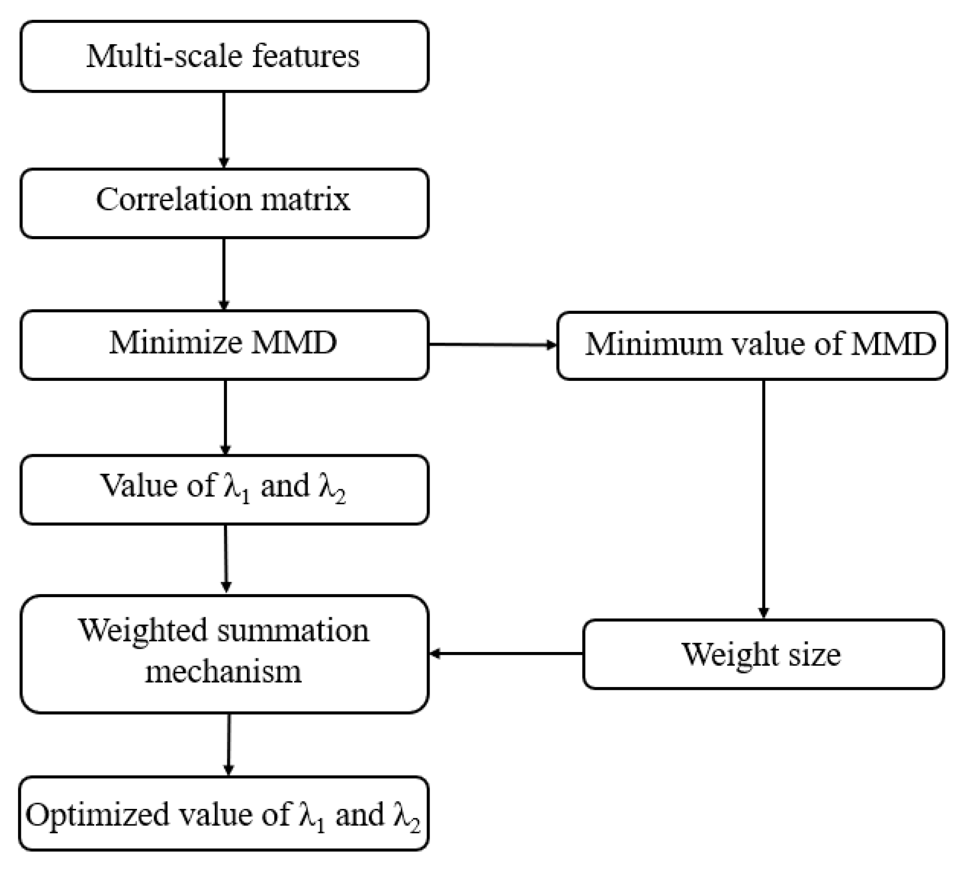
However, although it has been proven that the transfer kernel is PSD, it is often not effective when applied directly to the KELM. Therefore, it is necessary to optimize the transfer kernel to further optimize the inter-domain feature matching. Thereby, SFTKOS, as shown in Figure 2, is proposed. First of all, a parallel structure is designed to support multi-scale feature extraction to more fully characterize the state of vibration signals. Then, the correlation of inter-domain data sets is calculated according to the transfer kernel. Furthermore, the minimization MMD method is employed to optimize the transfer kernel to obtain the values of parameter ${\lambda }_1$ and ${\lambda }_2$. Finally, the optimized kernel function $K_{opt}$ is computed by the weighted fusing mechanism according to the minimization MMD size.

3.2. Training the Model

3.2.1. The Domain-Invariant Feature Extraction

In this study, a combination of functional principal component analysis and maximum mean difference methods (FPCA-MMD) was designed to extract domain-independent tracking indicators from bearing time-domain data. According to the literature [29], when processing high-dimensional time domain signals, FPCA can treat the data as a continuous function, so as to effectively capture potential degradation characteristics and reveal the trend in the degradation process. However, FPCA itself has limitations, such as the inability to directly measure statistical differences between different time periods, and the lack of clear quantification of dynamic changes in different degradation stages.

Therefore, FPCA-MMD combined with the MMD method can make up for this shortcoming of FPCA. MMD can effectively measure the difference in distribution between different time periods or degradation stages, thereby helping to reveal the dynamic changes in the degradation process. Specifically, FPCA first analyzes multi-dimensional data and extracts the features that can represent the main changes in the degradation process. These characteristics help us understand the main trends of degradation. Meanwhile, MMD is employed to measure the differences in the characteristic distribution at different degradation stages. By calculating these differences, we can quantify the changes between different stages, thereby more clearly identifying the key nodes in the degradation process. Therefore, to capture the relevant characteristics from bearing data in the time domain, FPCA-based dimensionality reduction is applied, resulting in a feature vector ${\mathit{x}}_{fpca}=\left[x_0,x_1,\dots ,x_n\right]$ that characterizes the bearing’s degradation. A sliding window technique [30] with step size $s$ is then employed to partition the feature set, producing subsets ${\mathit{x}}_w=\left[x_0^{\prime },x_1^{\prime },\dots ,x_{n-s}^{\prime }\right]$, in which ${\mathit{x}}^{\prime }=\left[x_0,x_1,\dots ,x_s\right]$. To analyze the changes in the degradation process, the variation difference between each subset and the initial one is computed. The difference value is quantified by the MMD method as follows:

$$D=MMD\left({\mathit{x}}_0^{\prime },{\mathit{x}}_k^{\prime }\right)$$

(13)

where $x_k^{\prime }$ denotes the data segment corresponding to the sliding window, and $k$ represents the index of the segment. The MMD function described in Section 2 is utilized to generate a series of difference values $D_w=\left(D_0,D_1,\dots ,D_{n-s}\right)$. These values are fed into the TK-KELM model as input to track bearing degradation.

3.2.2. KELM Model Training

Because the kernel function needs to meet the Mercer condition, it is also possible to use the new transfer kernel proposed above. Thus, KELM based on transfer kernel is named as TK-KELM in this work. At the same time, the structure of the new model is still consistent with the KELM model. Therefore, the new transfer kernel can be expressed as follows:

$${\mathit{K}}_{opt}=\mathit{H}{\mathit{H}}^T,K_{opt}\left(x_i,x_j\right)=h(x_i)h\left(x_j\right)$$

(14)

Thereby, the new output in this case is given by the following:

$$f_{TK-KELM}\left(x\right)=h\left(x\right){\mathit{H}}^T{\left({\mathit{K}}_{opt}+{\displaystyle \frac{1}{C}}\right)}^{-1}T$$

(15)

Then, the model output weight is solved as follows:

$$\beta ={\left({\displaystyle \frac{I}{C}}+{\mathit{K}}_{opt}^T{\mathit{K}}_{opt}\right)}^{-1}{\mathit{K}}_{opt}^{T}T$$

(16)

And finally, the predicted output can also be expressed as an expression that is only related to the kernel matrix. Then, the degradation indicator can be taken as the input of the model, and the predicted label data is used as a supplement to the insufficient target domain sample.

3.3. Condition Monitoring and Fault Diagnosis

Accurate monitoring of the degradation stage and early identification of faults are critical for BCM and BFD. The process of condition monitoring consists of systematically appraising the operational state of equipment to spot early indicators of degradation. Early detection allows for timely intervention, potentially preventing catastrophic failures. Fault diagnosis, on the other hand, involves identifying the specific nature and cause of a failure once it has occurred, providing insights for corrective actions and optimizing maintenance strategies.

For identifying the condition change point, a gradient iterative partitioning algorithm is applied in this article. The gradient is used to evaluate the variations in the degradation signal. A sharp variation in the gradient indicates a significant change in condition monitoring, which can be detected as a change point. The gradient at each instance is calculated as follows:

$$g_i={\displaystyle \frac{D_{i+1}-D_{i-1}}{2}}$$

(17)

where $g_i$ is the rate of change at that moment, that is, the gradient value. Additionally, a gradient threshold $G$ is set according to the 3σ principle. Based on the above settings, the objective of this paper is to identify the condition change points in the gradient. A change point is considered valid only when $g_i>G$ and the next $k$ consecutive gradient values satisfy $g_{i+k}>-G$. If these conditions are not met, the point is treated as a false change point.

After the identification of the failure points is completed, the core work of the next step is to deeply analyze these failure points to determine the specific nature behind them, and determine which fault types the fault points belong to. For fault diagnosis, a way of systematic implementation is designed as follows: First, the multi-scale features of vibration signals from both source and target domains are extracted using the transfer kernel optimized by SFTKOS. These features are then processed through the FPCA-MMD integration framework to derive domain-invariant degradation indicators, which serve as the input features for the classification model. Finally, the SVM is employed as the classifier, where the RBF is selected as the kernel function to handle the nonlinearity of the input features. The regularization parameter C of the SVM is determined via cross-validation within the range of 1 to 100 to balance the model’s generalization ability and classification accuracy.

The computational complexity of the proposed TK-KELM model is dominated by the kernel matrix construction and model training steps. For $n$ samples and $d$ feature dimensions, computational complexity for online monitoring is $O\left(n^2\right)+O\left(n\cdot d^2\right)+O\left(d^3\right)$, where $O\left(n^2\right)$ refers to the kernel matrix construction and model training steps; $O\left(n\cdot d^2\right)$ is the complexity of the covariance of d-dimensional features; and $O\left(d^3\right)$ represents the computational complexity of dimensionality reduction operations.

4. Case Study

In this section, the paper designs two empirical investigations to assess the effectiveness of the model in condition monitoring (Case 1), fault diagnosis (Case 2) and fault diagnosis in zero-faulty environments (Case 3), respectively.

4.1. Case 1: Bearing Condition Monitoring

4.1.1. Data Description

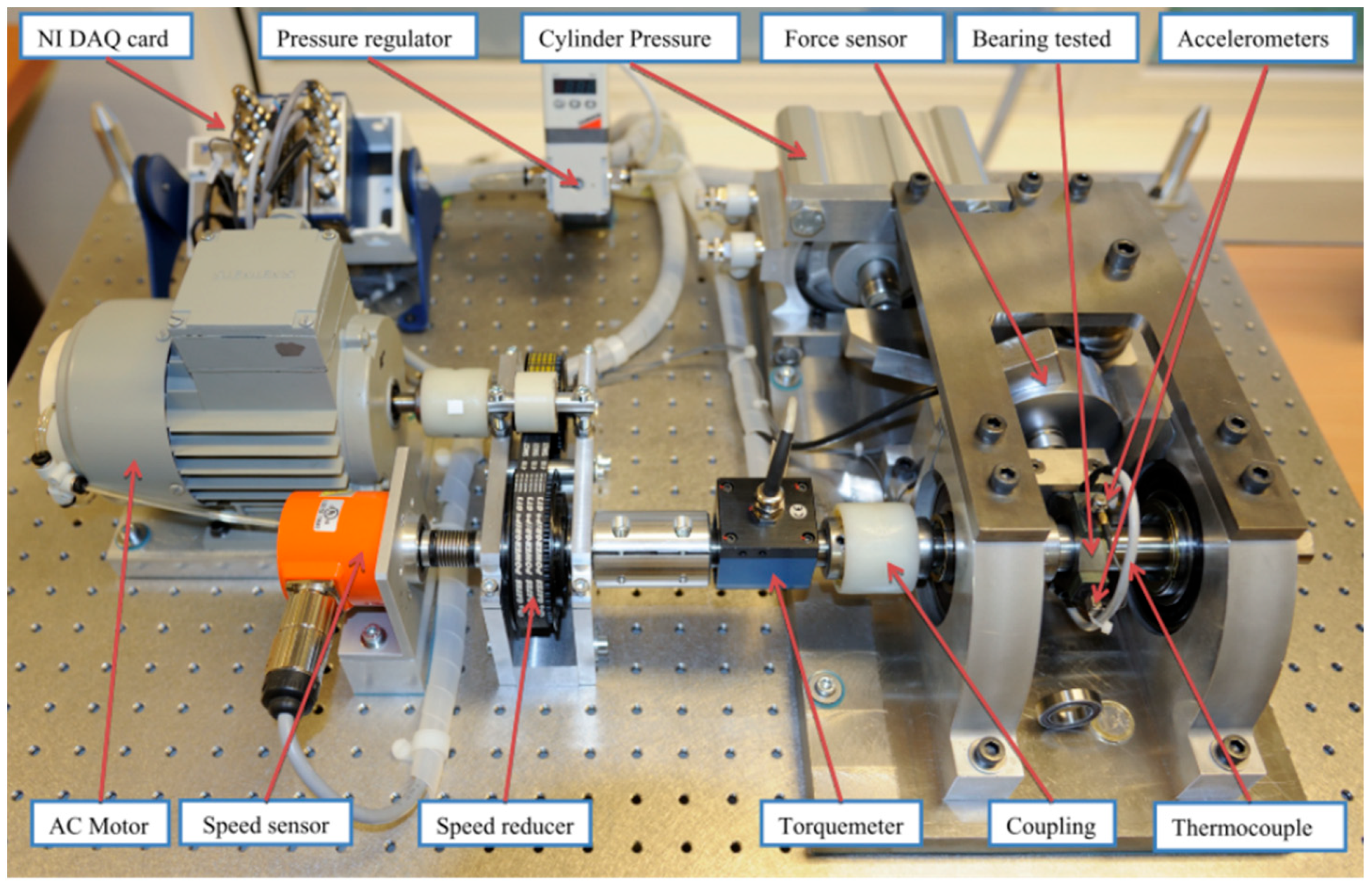
Figure 3 illustrates the experimental system in this paper, PRONOSTIA [31]. It was developed to evaluate methods for detecting bearing faults. The main contribution of this system is supplying authentic experimental data that track the wear and tear of rolling-element bearings throughout their full lifecycle, until complete failure. For example, this platform enables the degradation of bearings to be simulated in just a few hours, allowing for a large number of experiments to be conducted within a week. As a result, the dataset has been widely utilized by researchers as a benchmark for assessing condition monitoring approaches.

4.1.2. Task Setting

The working condition information of the PRONOSTIA data set is shown in

Table 1. The working condition information of the dataset.

Condition	Load	Speed	Bearing Number
One	4000 N	1800 rpm	Bearing 1–1, 1–2, 1–3, 1–4, 1–5, 1–6, 1–7
Two	4200 N	1650 rpm	Bearing 2–1, 2–2, 2–3, 2–4, 2–5, 2–6, 2–7
Three	5000 N	1500 rpm	Bearing 3–1, 3–2, 3–3

. This dataset contains three working conditions with different loads and rotational speeds, along with the corresponding bearing data sets. Some data were selected in this case for a controlled trial, as shown in

Table 2. The data set of the experiment.

Task	Training Set	Testing Set
A	Bearing 1–1	Bearing 2–3
B	Bearing 1–1	Bearing 3–2
C	Bearing 1–2	Bearing 2–3
D	Bearing 2–1	Bearing 1–3
E	Bearing 2–1	Bearing 3–3
F	Bearing 2–2	Bearing 1–3

.

4.1.3. Experimental Results

To quantify the differences in feature distribution, two statistical tests were used to verify the hypothesis of cross-domain shared degradation patterns: the Kolmogorov–Smirnov (KS) test and MMD. The quantification results are shown in

Table 3. The statistical quantification of feature distributions before transfer.

Task	KS p-Value	MMD Value
A	0.18	0.87
B	0.21	0.92
C	0.15	0.83
D	0.24	0.95
E	0.19	0.89
F	0.22	0.91

. All tasks produce KS test p-values $>0.05$, indicating the possibility that they have the same distribution. The MMD values of all tasks were $\ge 0.83$, indicating that the distribution differences before transfer processing were relatively large. These results statistically prove that the assumption of the cross-domain shared degradation model is correct.

To further validate the differences in feature distribution, the paper takes task A as an example: Figure 4 shows the t-SNE visualization of the feature distribution before and after transfer to illustrate the domain alignment effect more intuitively. Before transfer, the features of the source domain and the target domain are clearly separated. After the TK-KELM transfer, the features were well mixed, indicating that the model has a strong domain alignment ability.

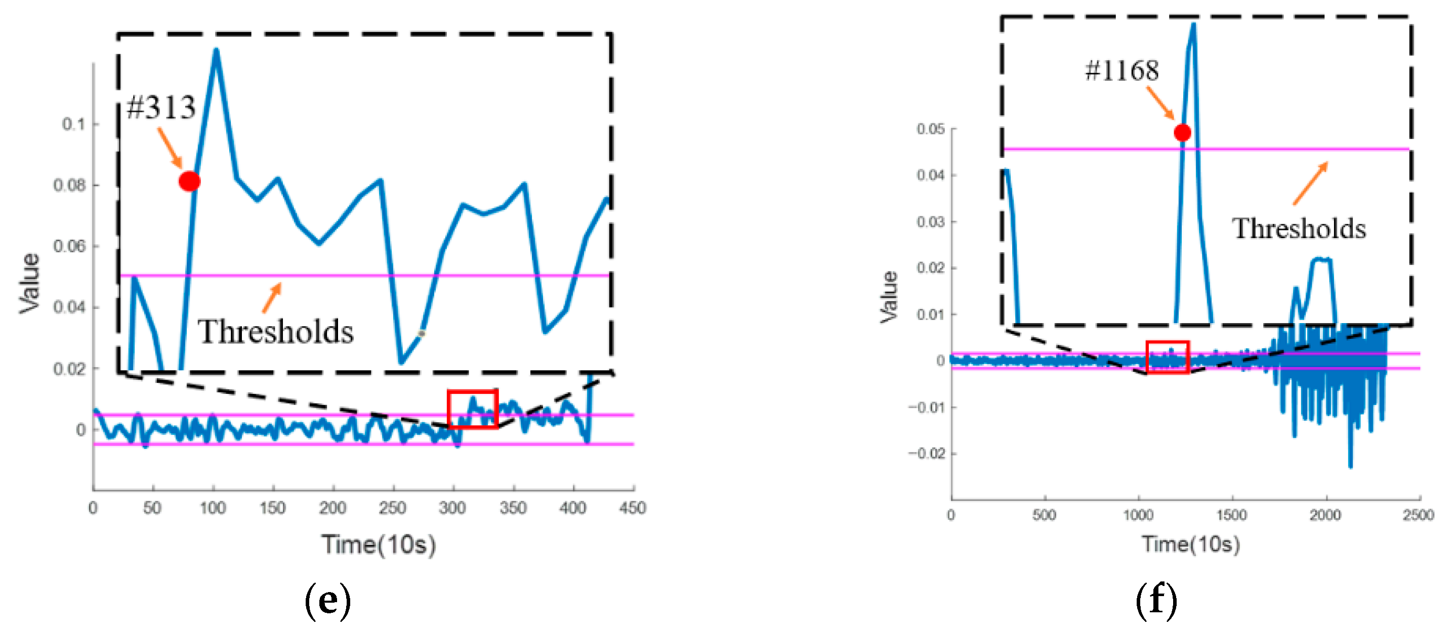
Figure 5 shows the condition monitoring performance of six experiments. For tasks A, B and tasks D, E with the same training dataset, they can all have a good cross-domain migration performance when facing different test datasets. For tasks A, C and tasks D, E with different training datasets, it can be observed that the obtained state change points are almost the same when facing the same set of test datasets, which indicates that the model has good generalization performance. Meanwhile, the tracking index obtained by using the data under working condition one as the source domain is more stable. The reason for the preliminary analysis is that the source domain data is more abundant, enabling the model to better capture the correlation and achieve better transfer performance. For Task B and Task E, they respectively trained the model using the training datasets under different working conditions, and at the same time monitored the test datasets under the third working condition. Both achieved good results.

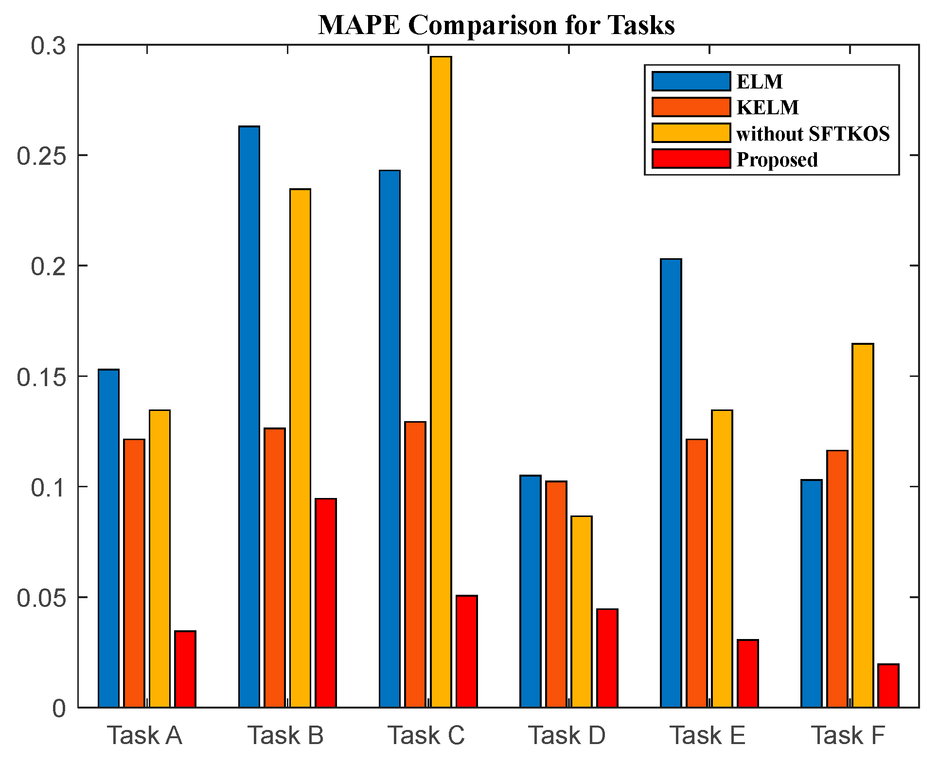
To demonstrate the performance of the proposed model in condition monitoring more clearly, the mean absolute percentage error (MAPE) metric was used. Figure 5 shows the comparison graph of MAPE of four models, ELM, KELM, without SFTKOS and the proposed model.

It is clear from the Figure 6 that the error of the proposed model is minimal. In the MAPE error analysis, the common KELM model is basically stable between 10% and 15% and the ELM model generally reaches 15% to 25%. However, the TK-KELM without SFTKOS model is much higher than the KELM model, with a large fluctuation between 10% and 30%, and even worse than the ELM model in some cases. As for the MAPE of the proposed model being maintained between 0 and 10%, it has a better migration performance compared with the other three models. It can be seen that the proposed SFTKOS is crucial for applying the transfer kernel to the KELM model, which greatly reduces model errors and improves model generalization.

4.1.4. Comparing Other Tests

The adaptability of the TK-KELM model is verified via a comparative study with respect to other condition monitoring algorithms. These comparison methods, including the gated recurrent unit-based health index (GRU-HI) [32], the two-level alarm mechanism (TLAM) [33], as well as the hidden Markov model (HMM) [34], comprising an unsupervised FPT detection model (USFPTD) [35] and multilayer cross-domain transformer network (MCTN) [36], are applied.

Table 4. The condition change point detection comparison.

	TK-KELM	GRU-HI	TLAM	HMM	USFPTD	MCTN
A	2480 s	2580 s	2600 s	2610 s	2510 s	2620 s
B	1640 s	2310 s	1650 s	3320 s	1660 s	14,210 s
C	2560 s	2610 s	2620 s	2610 s	2560 s	2620 s
D	11,360 s	13,650 s	14,330 s	15,340 s	11,780 s	18,420 s
E	3130 s	3480 s	3160 s	3160 s	3150 s	3160 s
F	11,680 s	13,760 s	14,620 s	16,840 s	11,710 s	18,460 s

gives a comparison of the condition change point locations identified in tasks A-F among the proposed method and other competing degradation models or detection algorithms. For the purpose of comparative analysis, the condition change point determined by the proposed model is relatively advanced. Especially compared with the new health index, GRU-HI, the degradation indicator extracted by the FPCA-MMD method in this paper can help us to monitor the change of bearing status earlier. Compared with MCTN and HMM, the TK-KELM model in this paper has obvious advantages for BCM. For the other two detection algorithms, TLAM and USFPTD, TLAM performs poorly, but USFPTD performs well. For task C, the change point detected by USFPTD was consistent with those detected by the approach presented here, and similar outcomes were obtained for other tasks. In summary, the TK-KELM model demonstrated strong performance in cross-domain BCM tasks, and the bearing degradation index extracted by the FPCA-MMD method is of significant help to BCM tasks.

4.2. Case 2: Bearing Fault Diagnosis

4.2.1. Data Description

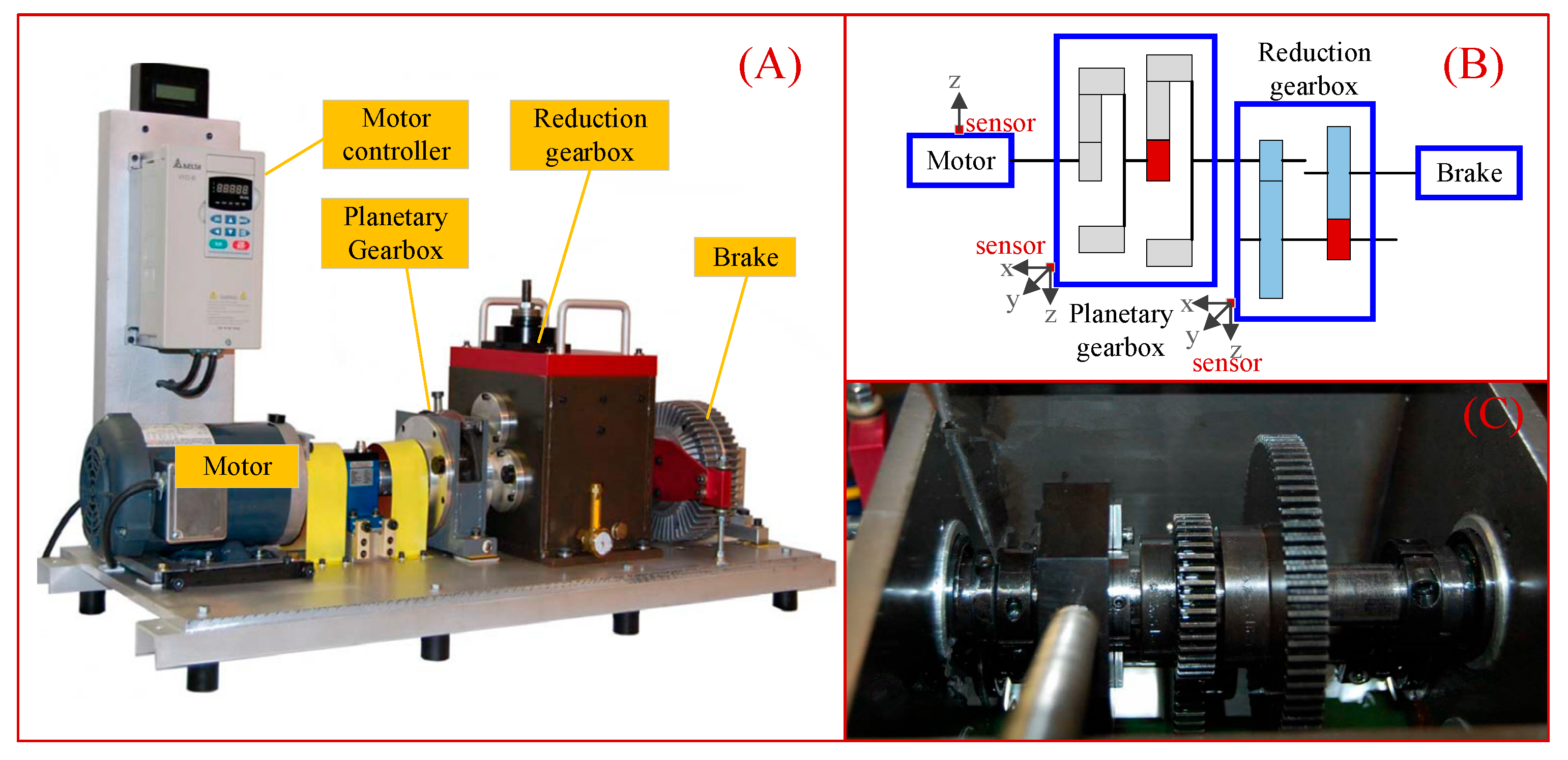
The SEU mechanical dataset [37] contains data related to the health and fault data for roll bearings, collected using the Drivetrain Dynamics Simulator (DDS), which is shown in Figure 7. The bearing data sets are captured with a frequency of 5120 Hz. As shown in

Table 5. Description of the data set used in the experiment.

Rotational speed (Hz)	D1: 20	D2: 30	D3: 40
Torque (N·m)	L1: 0	L2: 1	L3: 2
Fault location	DE (Drive end)

, these records span a range of operating conditions, different speeds and loads, including health and damage states. These conditions are classified into five categories: Normal (health element), Ball (issues with the rolling element), Inner (problems in the inner raceway), Outer (problems in the outer raceway), and Com (issues in both the inner and outer raceways simultaneously).

4.2.2. Task Setting

As shown in

Table 6. The data set of the experiment.

Transfer Task	Source Domain	Target Domain
A	D1, L1	D2, L1
B	D1, L1	D3, L1
C	D2, L1	D2, L2
D	D2, L1	D2, L3
E	D1, L1	D2, L3
F	D2, L2	D3, L1

, some transfer tasks were set for three different rotational speeds and three different loads, where the rotational speeds are set to D1, D2 and D3 and the system load configurations are set to set to L1, L2 and L3. In the tasks, the target samples were 1000 samples, including all types of faults (e.g., 200 samples for each type of fault). Additionally, the details of the parameter settings are as follows.

The regularization parameter C in the TK-KELM model is set to 10. The bandwidth σ of the RBF kernel is set to 1.5. The length of the sliding window is 2048 points and the step size is 1024 points. Additionally, each sample is constructed by fusing four time-domain features.

4.2.3. Experimental Results

To enhance the transparency and repeatability of the experiments, the sensitivity of these hyperparameters is studied. Take the task A as an example: Figure 8a shows the F1-score of the TK-KELM model with changing hyperparameters (e.g., ${\lambda }_1$ and ${\lambda }_2$, where ${\lambda }_2={\lambda }_1^2+0.1$). With the increase in ${\lambda }_1$, it can be seen from the figure that the F1-score keeps increasing at the beginning, and reaches the maximum value when ${\lambda }_1$ falls in 3.42. After that, F1-score dips from 0.977 to 0.904. Similarly, in Figure 8b, the F1-score first increases with sigma to 0.972 and then decreases to 0.84 to reach stability.

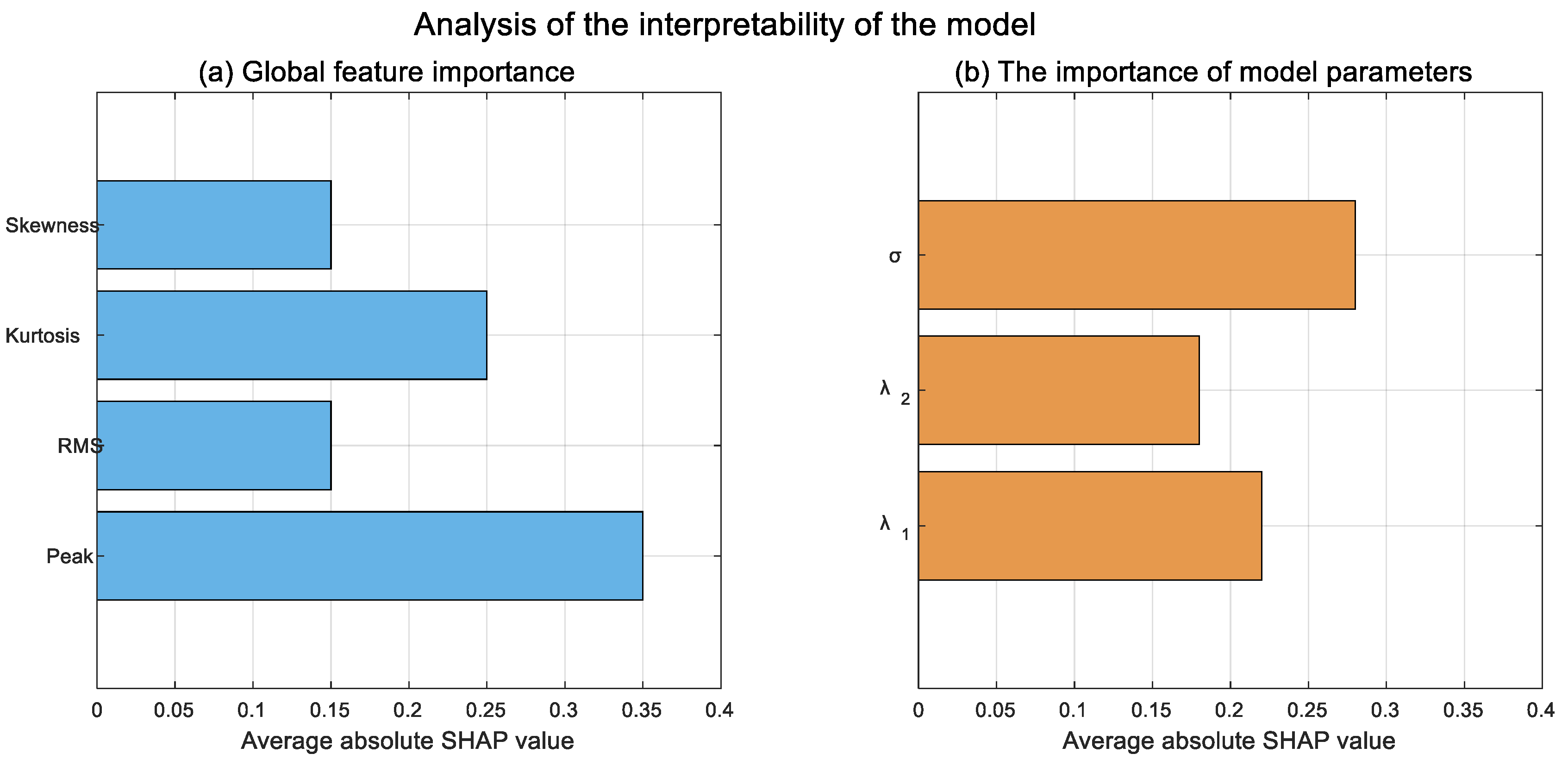
Figure 9a shows the average absolute SHAP values of skewness, kurtosis, root mean square and peak. The higher the SHAP value, the greater the contribution of features to the model’s decision-making. Faults can cause periodic impacts on the vibration signal. When the model detects an abnormally elevated peak value of the target domain samples (combined with the transfer kernel parameter to determine the inter-domain differences), it will prioritize the determination of a fault. The SHAP value of Kurtosis ranks second, corresponding to the compound fault scenario of bearing failure. Normal vibration signals follow an approximately Gaussian distribution. However, compound faults can lead to an asymmetric distribution of “spikes and long tails” in the signals. When the model detects Kurtosis anomalies, it will enhance the discrimination of compound faults. The energy level of the vibration signal reflected by RMS can be used as a preliminary judgment of the existence of faults. The asymmetry of the signal distribution quantified by Skewness may cause Skewness to show abnormalities before Peak and Kurtosis in the early stage of minor faults.

Figure 9b reveals how hyperparameters guide decisions: Kernel bandwidth $\sigma$ is critical. $\sigma$ determines the width of the RBF kernel function. The smaller $\sigma$, the more the kernel function focuses on local feature differences. The larger $\sigma$, the more attention is paid to the global feature distribution. ${\lambda }_1$ and ${\lambda }_2$ are associated with intra-domain and inter-domain weights. When the inter-domain differences are large, ${\lambda }_1$ can be greater than 1 to enhance the inter-domain alignment strength. When the inter-domain differences are small, ${\lambda }_1$ can be less than 1 to retain more intra-domain features.

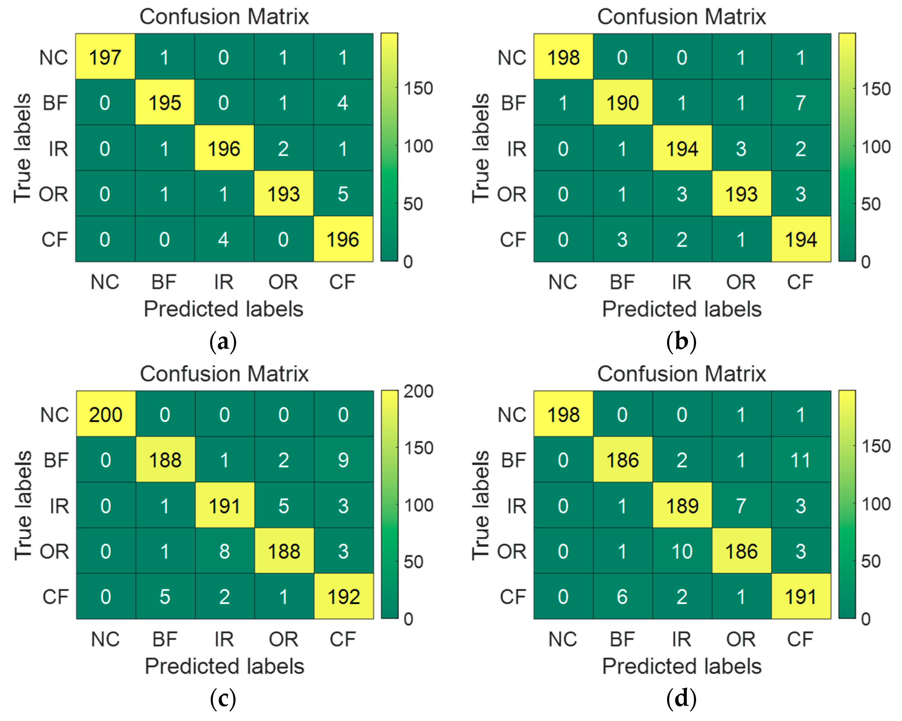
The diagnostic effectiveness of the proposed TK-KELM model on different cross-domain BFD tasks is represented through confusion matrices, as shown in Figure 10. In the confusion matrices, the actual fault categories are represented by rows, while the predicted fault categories are represented by columns. Overall, the model performed well in the six cross-domain transfer learning tasks, with task A and task B having the highest accuracy, followed by task C and task D, and finally task E and task F. It can be found that the performance of the proposed model is better in the case of different speeds than in the case of different loads.

In order to effectively illustrate the classification results, three indicators were used: accuracy rate (Precision), recall rate (Recall), and overall index of comprehensive evaluation (F1-score).

The corresponding calculation formula is as follows:

$$Precison ={\displaystyle \frac{True}{True+FP}}$$

(18)

$$Recall={\displaystyle \frac{True}{True+FN}}$$

(19)

$$F1={\displaystyle \frac{2\ast Precison \ast Recall}{Precison+Recall}}$$

(20)

where $True$ represents the number of samples for which both the real and predicted labels are $k$ and $FP$ represents the count of samples where the predicted label is $k$ but the actual label differs. $FN$ refers to the number of samples whose real label is $k$ while its prediction label is different from $k$.

To ensure the reliability and robustness of the proposed TK-KELM model, 10-fold cross-validation was meticulously conducted across all tasks (A–F). As presented in

Table 7. The 10-fold cross-validation results.

Task	Average F1-Score	Standard Deviation (σ)	Best Fold F1-Score	Worst Fold F1-Score
A	0.977	0.012	0.991	0.958
B	0.969	0.015	0.985	0.947
C	0.959	0.018	0.976	0.933
D	0.950	0.021	0.968	0.925
E	0.944	0.023	0.962	0.919
F	0.936	0.025	0.955	0.907

, the TK-KELM model demonstrates remarkable stability, with low standard deviations ($\sigma <0.025$ for all tasks).

4.2.4. Comparing Other Tests

To demonstrate the superiority of the TK-KELM model, this model is compared with other approaches for transfer learning: transfer component analysis (TCA) [38], joint distribution adaptation (JDA) [39], domain adaptive neural network (DANN) [40], multi-representation adaptation network (MRAN) [41], deep convolutional transfer learning network (DCTLN) [42], contrastive learning (CL) [43], deep correlation alignment (Deep CORAL) [44] maximum classifier discrepancy (MCD) [45], shrinkage mamba relation network (SMRN) and relation network (RN) [26].

As shown in

Table 8. Comparison of diagnostic F1-score.

Method	Task A	Task B	Task C	Task D	Task E	Task F	Average
Proposed	0.977	0.969	0.959	0.950	0.944	0.936	0.956
TCA	0.626	0.624	0.633	0.662	0.632	0.688	0.644
JDA	0.721	0.726	0.733	0.768	0.735	0.773	0.742
MRAN	0.804	0.726	0.774	0.723	0.687	0.822	0.756
DANN	0.768	0.782	0.812	0.705	0.752	0.825	0.774
DCTLN	0.811	0.736	0.822	0.801	0.726	0.895	0.799
CL	0.732	0.741	0.802	0.680	0.729	0.813	0.750
Without SFTKOS	0.713	0.722	0.736	0.691	0.718	0.746	0.721
Without FPCA-MMD	0.746	0.759	0.774	0.703	0.733	0.757	0.745
Deep CORAL	0.823	0.815	0.831	0.792	0.804	0.842	0.818
MCD	0.754	0.762	0.778	0.745	0.751	0.783	0.762
SMRN	0.805	0.776	0.784	0.785	0.763	0.788	0.784
RN	0.754	0.767	0.765	0.756	0.744	0.782	0.761

, it is found that the average F1-score of the proposed method achieved 0.956. This performance was significantly better than that of TCA (0.644), JDA (0.742), MRAN (0.756), DANN (0.774), DCTLN (0.799), CL (0.750), without SFTKOS (0.721) and without FPCA-MMD (0.745). In a further analysis of these results, both TCA and JDA use Gaussian kernel function, but they are more focused on reducing edge inter-domain distribution differences. On the contrary, the proposed similarity-based feature-directed transfer kernel optimization method is used in this paper to make the kernel function adjust according to the similarity characteristics of inter-domain data sets, so that the inter-domain similar samples are more closely aligned in the high-dimensional space, improving the transfer performance. MRAN can deal with the alignment problem of different modes or features more comprehensively through multiple representation learning, so it performs well in multi-modal cross-domain tasks. However, the treatment of the nonlinear relationship between features is still rough. DANN’s adversarial data processing involves competition between feature extractors and domain discriminators, resulting in feature representations that are both class discriminant and domain invariant. Despite DANN enhancing the transfer ability of features, it also reduces the discriminability of features. While DCTLN shows decent performance, it may not fully exploit the underlying similarities between domains that are necessary for improving transfer performance in more challenging scenarios. Although CL is powerful in representation learning, especially in unsupervised settings, it does not explicitly account for domain alignment between source and target. In the absence of SFTKOS or FPCA-MMD, the F1-score of the model diagnosis results decreased significantly. Deep CORAL only aligns second-order statistics and has difficultly capturing the distribution differences of complex faults. MCD relies on classifier differential-driven adaptation and has insufficient robustness against multi-task domain offsets of bearing faults. Therefore, the TK-KELM model stands out because it uses the transfer kernel to process nonlinear data, employs an effective transfer kernel optimization method to further optimize the transfer kernel and simultaneously utilizes the FPCA-MMD method to extract multi-scale and invariant features and build the degradation tracking indicator.

To further validate the practicality of the proposed TK-KELM in zero-faulty bearing fault diagnosis, especially for industrial real-time deployment,

Table 9. Comparison of computational efficiency.

Method	Training Time (s)	Single-Sample Prediction Time (ms)	Memory Usage (MB)	GPU or CPU	CPU Usage (%)
Proposed	9.6 ± 0.4	0.14 ± 0.02	482 ± 22	CPU	20 ± 3
TCA	6.8 ± 0.3	0.09 ± 0.01	395 ± 18	CPU	15 ± 2
JDA	12.3 ± 0.5	0.18 ± 0.03	520 ± 25	CPU	22 ± 4
MRAN	35.7 ± 1.1	0.75 ± 0.05	1180 ± 45	CPU	48 ± 6
DANN	89.5 ± 2.8	1.2 ± 0.08	2450 ± 70	GPU	68 ± 8
DCTLN	156.2 ± 4.2	1.85 ± 0.12	3820 ± 90	GPU	78 ± 10
CL	72.4 ± 3.0	0.95 ± 0.06	1980 ± 60	GPU	55 ± 7
Deep CORAL	42.5 ± 1.5	0.82 ± 0.07	1350 ± 50	CPU	35 ± 5
MCD	58.3 ± 2.1	1.05 ± 0.09	1720 ± 65	GPU	48 ± 6

adds computational efficiency metrics, which are training time, single-sample prediction time, memory usage and CPU/GPU dependency. All experiments are conducted on a unified hardware platform (Intel Core i7-10700K CPU @ 3.80 GHz, NVIDIA RTX 3090). Runtime is averaged over 10 independent trials to ensure reliability. The proposed TK-KELM demonstrates superior computational efficiency for zero-faulty bearing diagnosis. With a training time of 9.6 ± 0.4 s, it is slightly slower than lightweight TCA but far faster than deep learning methods (DANN: 89.5 ± 2.8 s; DCTLN: 156.2 ± 4.2 s) and MRAN (35.7 ± 1.1 s). Its single-sample prediction time (0.14 ± 0.02 ms) meets real-time needs. TK-KELM consumes 482 ± 22 MB memory with 20 ± 3% CPU load, far lower than GPU methods. Balancing accuracy and efficiency, it suits industrial real-time deployment.

4.3. Case 3: Bearing Fault Diagnosis in the Zero-Faulty Environment

To address the zero-fault scenario, where the target domain lacks fault data, this paper integrates the deep convolutional generative adversarial networks (DCGAN) [46] and out-of-distribution data augmentation (OOD-DA) [26] with the proposed TK-KELM model, respectively. The core idea is to generate pseudo-fault samples consistent with the data distribution of the target domain by using the fault knowledge of the source domain, so as to conduct effective fault diagnosis when the fault data of the target domain is unavailable.

4.3.1. Data Description

For the zero-fault environment verification, vibration data from the Paderborn [47] was used, which is shown in Figure 11. The dataset encompasses signal data from three types of bearings: healthy bearings, bearings with artificial damage and bearings with realistic damage. All these bearings operated under three distinct load conditions, shown in

Table 10. The settings of Paderborn platform.

Name of Settings	Bearing Condition	Load Torque (Nm)	Radial Force (N)	Motor Speed (rpm)
L1	Normal, Inner, Outer	0.1	1000	1500
L2		0.7	400	1500
L3		0.7	1000	1500
L4		0.7	1000	900

, and at a rotational speed of 1500 rpm. For each bearing under a specific load setting, a vibration signal lasting roughly 4 s was measured. With a sampling rate of 64 kHz, each measurement resulted in a total of about 256,000 data points.

4.3.2. Task Setting

Table 11. The transfer tasks in zero-faulty environment.

Task	Source	Target
A	L1	L2
B	L1	L3
C	L2	L3
D	L3	L4
E	L4	L1
F	L4	L2

presents three transfer tasks, namely task A, task B and task C, which simulate the transfer of source domain knowledge to the target domain with different fault diameters. As shown in

Table 12. The data set of the transfer tasks in zero-faulty environment.

Label	Health Conditions	Source Sample Size	Target Sample Number
			Training Set	Testing Set
Normal	Normal working condition	1000	250	200
PF	Pseudo fault	1000	50	0
Outer	Outer ring fault	1000	0	200
Inner	Inner ring fault	1000	0	200

, there are 1000 samples for each type of source domain. To achieve a zero-fault environment, the training samples for the target domain consist of only 250 normal samples and 50 pseudo-fault samples generated by DCGAN and OOD-DA. The test samples for the target domain have 200 samples for each type of fault.

4.3.3. Comparing Other Tests

Table 13. Comparison of diagnostic F1-score in zero-faulty environment.

Method	Task A	Task B	Task C	Task D	Task E	Task F	Average
Proposed with DCGAN	0.987	0.994	0.962	0.975	0.982	0.979	0.980
Proposed with OOD-DA	0.998	1.0	1.0	1.0	0.992	1.0	1.0
TCA	0.524	0.552	0.538	0.516	0.541	0.529	0.533
JDA	0.581	0.563	0.602	0.574	0.590	0.586	0.583
MRAN	0.932	0.926	0.907	0.918	0.929	0.921	0.922
DANN	0.938	0.955	0.920	0.931	0.943	0.936	0.937
DCTLN	0.965	0.982	0.946	0.958	0.971	0.962	0.964
CL	0.633	0.619	0.703	0.647	0.668	0.655	0.654
Without SFTKOS	0.743	0.766	0.725	0.732	0.755	0.748	0.745
Without FPCA-MMD	0.864	0.892	0.827	0.851	0.876	0.868	0.863
Deep CORAL	0.895	0.913	0.876	0.889	0.902	0.897	0.895
MCD	0.812	0.835	0.798	0.806	0.823	0.817	0.815
SMRN	0.852	0.871	0.843	0.865	0.859	0.868	0.860
RN	0.837	0.854	0.829	0.846	0.838	0.849	0.842

clearly demonstrates that the proposed TK-KELM model achieves exceptional performance in zero-fault environments by using OOD-DA. This outstanding result validates the effectiveness of the model’s integrated design: by combining pseudo-fault samples generated by OOD-DA with the transfer kernel mechanism, it successfully overcomes the challenge of scarce fault data in target domains. Traditional methods, such as TCA (0.538) and JDA (0.582), struggle here, as their heavy dependence on explicit fault features causes poor generalization when target domain training lacks real faults. Similarly, in the absence of FPCA-MMD and SFTKOS, it is difficult to train the model effectively. TK-KELM and other deep learning models utilize the pseudo faults generated by DCGAN as a bridge to compensate for the scarcity of fault data in the target domain. Although these pseudo faults are not real, they can help the model learn the boundary between normal and abnormal states. In contrast, methods like CL, which lack effective mechanisms to handle scenarios with scarce faults, cannot extract discriminative features from the limited normal data, resulting in a lower F1-scosre. Despite leveraging Mamba for sequence modeling, SMRN and RN are constrained by the reliance on source data alone, lacking pseudo-fault augmentation to generalize to unseen target-domain fault patterns.

5. Conclusions

This paper proposes a novel transfer kernel enabled kernel extreme learning machine (TK-KELM) model for bearing fault diagnosis and condition monitoring. It addresses the problem of ignoring intra-domain relationships and limiting the range of weighting parameters describing inter-domain relationships in cross-domain scenarios. Experimental results show that the TK-KELM method is superior to conventional methods in accuracy, and can be more effective in BCM and BFD. Although the proposed TK-KELM model performs well, it is important to recognize its current limitations. In Case 3, The current reliance on DCGAN-generated pseudo faults may restrict generalization to unseen real fault types, as synthetic samples cannot fully replicate the complexity of actual fault characteristics. Secondly, the model’s adaptability to varying operating conditions is limited, with performance fluctuating across different settings as observed in Case 2. To address these limitations, future efforts will focus on developing adaptive normal pattern learning mechanisms, as well as designing adaptive transfer mechanisms that can dynamically adjust to varying operating conditions to reduce dependence on pseudo-fault samples and mitigate performance fluctuations across different settings.

References

1. Choi, K.; Yi, J.; Park, C.; Yoon, S. Deep Learning for Anomaly Detection in Time-Series Data: Review, Analysis, and Guidelines. IEEE Access 2021, 9, 120043–120065. [Google Scholar] [CrossRef]
2. Cao, H.; Niu, L.; Xi, S.; Chen, X. Mechanical model development of rolling bearing-rotor systems: A review. Mech. Syst. Signal Process. 2018, 102, 37–58. [Google Scholar] [CrossRef]
3. Truong, C.; Oudre, L.; Vayatis, N. Selective review of offline change point detection methods. Signal Process. 2020, 167, 107299. [Google Scholar] [CrossRef]
4. Zhang, Q.; Chen, Q.; Xu, L.; Xu, X.; Liang, Z. Wheat Lodging Direction Detection for Combine Harvesters Based on Improved K-Means, Bag of Visual Words. Agronomy 2023, 13, 2227. [Google Scholar] [CrossRef]
5. Patacchiola, M.; Turner, J.; Crowley, E.J.; Storkey, A.J. Bayesian Meta-Learning for the Few-Shot Setting via Deep Kernels. Adv. Neural Inf. Process. Syst. 2020, 33, 16108–16118. [Google Scholar]
6. Huang, S.; Cai, N.; Narrandes, S.; Wang, Y.; Xu, W. Applications of Support Vector Machine (SVM) Learning in Cancer Genomics. Cancer Genom. Proteom. 2018, 15, 41–51. [Google Scholar]
7. Xu, J.; Fang, M.; Zhao, W.; Fan, Y.; Ding, X. Deep Transfer Learning Remaining Useful Life Prediction of Different Bearings. In Proceedings of the International Joint Conference on Neural Networks, Shenzhen, China, 18–22 July 2021; pp. 1–8. [Google Scholar]
8. Antoni, J.; Borghesani, P. A statistical methodology for the design of condition indicators. Mech. Syst. Signal Process. 2019, 114, 290–327. [Google Scholar] [CrossRef]
9. Chen, B.; Cheng, Y.; Cao, H.; Song, S.; Mei, G.; Gu, F.; Zhang, W.; Ball, A.D. Generalized Statistical Indicators-Guided Signal Blind Deconvolution for Fault Diagnosis of Railway Vehicle Axle-Box Bearings. IEEE Trans. Veh. Technol. 2025, 74, 2458–2469. [Google Scholar] [CrossRef]
10. Chen, B.; Cheng, Y.; Allen, P.; Wang, S.; Gu, F.; Zhang, W.; Ball, A.D. A product envelope spectrum generated from spectral correlation/coherence for railway axle-box bearing fault diagnosis. Mech. Syst. Signal Process. 2025, 225, 112262. [Google Scholar] [CrossRef]
11. Zhou, X.; Sun, J.; Tian, Y.; Lu, B.; Hang, Y.; Chen, Q. Hyperspectral technique combined with deep learning algorithm for detection of compound heavy metals in lettuce. Food Chem. 2020, 321, 126503. [Google Scholar] [CrossRef]
12. Tsung, F.; Zhang, K.; Cheng, L.; Song, Z. Statistical transfer learning: A review and some extensions to statistical process control. Qual. Eng. 2017, 30, 115–128. [Google Scholar] [CrossRef]
13. Yan, T.; Wang, D.; Hou, B.; Peng, Z. Generic Framework for Integration of First Prediction Time Detection with Machine Degradation Modelling from Frequency Domain. IEEE Trans. Reliab. 2022, 71, 1464–1476. [Google Scholar] [CrossRef]
14. Chen, C.; Zhu, W.; Steibel, J.; Siegford, J.; Han, J.; Norton, T. Classification of drinking, drinker-playing in pigs by a video-based deep learning method. Biosyst. Eng. 2020, 196, 1–14. [Google Scholar] [CrossRef]
15. Hu, Q.; Si, X.; Qin, A.; Lv, Y.; Liu, M. Balanced Adaptation Regularization Based Transfer Learning for Unsupervised Cross-Domain Fault Diagnosis. IEEE Sens. J. 2022, 22, 12139–12151. [Google Scholar] [CrossRef]
16. Ganin, Y.; Ustinova, E.; Ajakan, H.; Germain, P.; Larochelle, H.; Laviolette, F.; Marchand, M.; Lempitsky, V. Domain-adversarial training of neural networks. J. Mach. Learn. Res. 2016, 17, 1–35. [Google Scholar]
17. Ganin, Y.; Kulkarni, T.; Babuschkin, I.; Ali Eslami, S.M.; Vinyals, O. Synthesizing Programs for Images using Reinforced Adversarial Learning. In Proceedings of the Machine Learning Research, Stockholm, Sweden, 10–15 July 2018; pp. 1666–1675. [Google Scholar]
18. Radhakrishnan, A.; Ruiz Luyten, M.; Prasad, N.; Uhler, C. Transfer Learning with Kernel Methods. Nat. Commun. 2023, 14, 55–70. [Google Scholar] [CrossRef]
19. Cao, B.; Pan, S.J.; Zhang, Y.; Yeung, D.; Yang, Q. Adaptive transfer learning. In Proceedings of the AAAI Conference on Artificial Intelligence, Atlanta, GA, USA, 11–15 July 2010; pp. 407–712. [Google Scholar]
20. Wagle, N.; Frew, E.W. Forward Adaptive Transfer of Gaussian Process Regression. J. Aerosp. Inform. Syst. 2017, 14, 214–231. [Google Scholar] [CrossRef]
21. Wei, P.; Vo, T.V.; Qu, X.; Ong, Y.S.; Ma, Z. Transfer Kernel Learning for Multi-Source Transfer Gaussian Process Regression. IEEE Trans. Pattern Anal. Mach. Intell. 2023, 45, 3862–3876. [Google Scholar] [CrossRef] [PubMed]
22. Wei, P.; Sagarna, R.; Ke, Y.; Ong, Y.-S. Practical Multisource Transfer Regression with Source–Target Similarity Captures. IEEE Trans. Neural Netw. Learn. Syst. 2021, 32, 3498–3509. [Google Scholar] [CrossRef]
23. Zheng, X.; Fan, W.; Chen, C.; Peng, Z. Adaptive Two-Stage Model for Bearing Remaining Useful Life Prediction Using Gaussian Process Regression with Matched Kernels. IEEE Trans. Reliab. 2024, 73, 1958–1966. [Google Scholar] [CrossRef]
24. Lu, X.; Ma, Z.; Lin, Y. Domain Adaptive Learning Based on Sample-Dependent and Learnable Kernels. arXiv 2021, arXiv:2102.09340. [Google Scholar] [CrossRef]
25. Wu, Z.; Jiang, H.; Zhao, K.; Li, X. An adaptive deep transfer learning method for bearing fault diagnosis. Measurement 2020, 151, 107227. [Google Scholar] [CrossRef]
26. Chen, Z.; Huang, H.; Deng, Z.; Wu, J. Shrinkage mamba relation network with out-of-distribution data augmentation for rotating machinery fault detection and localization under zero-faulty data. Mech. Syst. Signal Process. 2025, 224, 112145. [Google Scholar] [CrossRef]
27. Huang, G.; Zhu, Q.; Siew, C. Extreme learning machine: Theory and applications. Neurocomputing 2006, 70, 489–501. [Google Scholar] [CrossRef]
28. Gretton, A.; Borgwardt, K.M.; Rasch, M.J.; Schölkopf, B.; Smola, A. A kernel two-sample test. J. Mach. Learn. Res. 2012, 13, 723–773. [Google Scholar]
29. Wei, Y.; Xiao, G.; Deng, H.; Chen, H.; Tong, M.; Zhao, G.; Liu, Q. Hyperspectral image classification using FPCA-based kernel extreme learning machine. Optik 2015, 126, 3942–3948. [Google Scholar] [CrossRef]
30. Li, Z.; Cheng, D.; Zhang, H.; Zhou, K.; Wang, Y. Multi-feature spaces cross adaption transfer learning-based bearings piece-wise remaining useful life prediction under unseen degradation data. Adv. Eng. Inform. 2024, 60, 102413. [Google Scholar] [CrossRef]
31. Nectoux, P.; Gouriveau, R.; Medjaher, K.; Ramasso, E.; Morello, B.; Zerhouni, N.; Varnier, C. PRONOSTIA: An Experimental Platform for Bearings Accelerated Life Test. In Proceedings of the 2025 IEEE International Conference on Prognostics and Health Management, Denver, CO, USA, 18–21 June 2012. [Google Scholar]
32. Xu, C.; Yang, K.; Chen, X.; Luo, X.; Yu, H. Transfer Learning for Regression through Adaptive Gaussian Process. In Proceedings of the International Conference on Tools for Artificial Intelligence, Macao, China, 31 October–2 November 2022; pp. 42–47. [Google Scholar]
33. Cheng, H.; Kong, X.; Wang, Q.; Ma, H.; Yang, S. The two-stage RUL prediction across operation conditions using deep transfer learning and insufficient degradation data. Reliab. Eng. Syst. Saf. 2022, 225, 108581. [Google Scholar] [CrossRef]
34. Zhu, J.; Chen, N.; Shen, C. A new data-driven transferable remaining useful life prediction approach for bearing under different working conditions. Mech. Syst. Signal Process. 2020, 139, 106602. [Google Scholar] [CrossRef]
35. Chen, K.; Liu, J.; Guo, W.; Wang, X. A two-stage approach based on Bayesian deep learning for predicting remaining useful life of rolling element bearings. Comput. Electr. Eng. 2023, 109, 108745. [Google Scholar] [CrossRef]
36. Zhang, Y.; Feng, K.; Yu, K.; Ji, J.C.; Ren, Z.; Liu, Z. Dynamic Model-Assisted Bearing Remaining Useful Life Prediction Using the Cross-Domain Transformer Network. IEEE ASME Trans. Mechatron. 2023, 28, 1070–1080. [Google Scholar] [CrossRef]
37. Shao, S.; McAleer, S.; Yan, R.; Baldi, P. Highly Accurate Machine Fault Diagnosis Using Deep Transfer Learning. IEEE Trans. Ind. Inf. 2019, 15, 2446–2455. [Google Scholar] [CrossRef]
38. Pan, S.; Tsang Ivor, W.; Kwok, J.T.; Yang, Q. Domain Adaptation via Transfer Component Analysis. IEEE Trans. Neural Netw. 2011, 22, 199–210. [Google Scholar] [CrossRef] [PubMed]
39. Han, T.; Liu, C.; Yang, W.; Jiang, D. Deep transfer network with joint distribution adaptation: A new intelligent fault diagnosis framework for industry application. ISA Trans. 2020, 97, 269–281. [Google Scholar] [CrossRef]
40. Ghifary, M.; Kleijin, W.B.; Zhang, M. Domain Adaptive Neural Networks for Object Recognition. arXiv 2014, arXiv:1409.6041. [Google Scholar] [CrossRef]
41. Zhu, Y.; Zhuang, F.; Wang, J.; Chen, J.; Shi, Z.; Wu, W.; He, Q. Multi-representation adaptation network for cross-domain image classification. Neural Netw. 2019, 119, 214–221. [Google Scholar] [CrossRef]
42. Guo, L.; Lei, Y.; Xing, S.; Yan, T.; Li, N. Deep Convolutional Transfer Learning Network: A New Method for Intelligent Fault Diagnosis of Machines With Unlabeled Data. IEEE. Trans. Ind. Electron. 2019, 66, 7316–7325. [Google Scholar] [CrossRef]
43. He, K.; Fan, H.; Wu, Y.; Xie, S.; Girshick, R. Momentum Contrast for Unsupervised Visual Representation Learning. arXiv 2020, arXiv:1911.05722v3. [Google Scholar] [CrossRef]
44. Li, X.; Zhang, Z.; Gao, L.; Wen, L. A New Semi-Supervised Fault Diagnosis Method via Deep CORAL and Transfer Component Analysis. IEEE Trans. Emerg. Top. Comput. Intell. 2022, 6, 690–699. [Google Scholar] [CrossRef]
45. Cho, J.W.; Kim, D.-J.; Jung, Y.; Kweon, I.S. MCDAL: Maximum Classifier Discrepancy for Active Learning. IEEE Trans. Neural Netw. Learn. Syst. 2023, 34, 8753–8763. [Google Scholar] [CrossRef]
46. Radford, A.; Metz, L.; Chintala, S. Unsupervised Representation Learning with Deep Convolutional Generative Adversarial Networks. arXiv 2016, arXiv:1511.06434. [Google Scholar] [CrossRef]
47. Lessmeier, C.; Kimotho, J.K.; Zimmer, D.; Sextro, W. Condition Monitoring of Bearing Damage in Electromechanical Drive Systems by Using Motor Current Signals of Electric Motors: A Benchmark Data Set for Data-Driven Classification. In Proceedings of the European Conference of the Prognostics and Health Management Society (PHM Society), Bilbao, Spain, 5–8 July 2016. [Google Scholar]
Figure 1. The overall block diagram of the proposed method.
Machines 13 00793 g001
Figure 2. The flow chart of SFTKOS.
Machines 13 00793 g002
Figure 3. Test platform of PRONOSTIA.
Machines 13 00793 g003
Figure 4. The visualizations of feature distributions before and after transfer.
Machines 13 00793 g004
Figure 5. The condition monitoring results of task A–F. (af) are the results of tasks A–F, respectively.
Machines 13 00793 g005aMachines 13 00793 g005b
Figure 6. The MAPE comparison of four models.
Machines 13 00793 g006
Figure 7. The test platform of DDS. (A) shows the overall structure of the test platform; (B) illustrates the schematic diagram of the system components; (C) presents the partial enlarged view of the gear transmission structure.
Machines 13 00793 g007
Figure 8. The sensitivity analysis. (a) depicts the sensitivity analysis of λ 1 and λ 2 with F1-score; (b) shows the sensitivity analysis of kernel bandwidth with F1-score.
Machines 13 00793 g008
Figure 9. The SHAP-based interpretability analysis.
Machines 13 00793 g009
Figure 10. The confusion matrices of task A–F. (af) are the results of tasks A–F, respectively.
Machines 13 00793 g010aMachines 13 00793 g010b
Figure 11. The platform of Paderborn bearing data.
Machines 13 00793 g011