Article

Multi-Source Error Coupling and Tolerance Optimization for Improving the Precision of Automated Assembly of Aircraft Components

College of Mechanical and Electrical Engineering, Nanjing University of Aeronautics and Astronautics, Nanjing 210016, China
*
Author to whom correspondence should be addressed.
Machines 2025, 13(8), 736; https://doi.org/10.3390/machines13080736
Submission received: 4 July 2025 / Revised: 13 August 2025 / Accepted: 14 August 2025 / Published: 19 August 2025
(This article belongs to the Section Automation and Control Systems)

Abstract

In automated aircraft assembly, achieving high-precision alignment is essential due to the presence of multiple coupled error sources that significantly affect final product quality. This study proposes an integrated framework to model multi-source errors via a directed coupling network and to quantify their impact using Monte Carlo simulations. To reduce the complexity of tolerance allocation, Sobol-based global sensitivity analysis is applied to identify dominant contributors to assembly deviations. The most influential parameters are retained for multi-objective optimization using the non-dominated sorting genetic algorithm II (NSGA-II). This framework enables the minimization of key assembly deviations while maintaining computational efficiency. Experimental validation on a typical helicopter ring assembly demonstrates that the proposed optimization approach increases the position pass rate from 67.4% to 100.0% and the coaxiality pass rate from 93.5% to 100.0%. The corresponding process capability indices (CPK) also improve significantly, from 0.31 to 2.19 for position and from 0.62 to 1.06 for coaxiality. These improvements not only satisfy high-precision assembly requirements but also exceed common industry benchmarks, demonstrating the method’s practical effectiveness under multi-source uncertainty.

1. Introduction

Modern military and commercial aircraft demand extremely tight assembly tolerances and efficiency. For example, automated drilling and riveting systems for aircraft panels have achieved a positioning accuracy of ±0.05 mm [1], far higher than typical manual assembly. As a result, original equipment manufacturers such as Boeing and Airbus are rapidly expanding the use of robotics and digital assembly [2]. For example, Airbus has opened a highly automated fuselage assembly line for the A320 aircraft in Hamburg [3,4], reflecting the industry’s trend of adopting robotics in high-volume aircraft production. These automation measures have brought significant benefits: (a) With increasing precision requirements in aerospace manufacturing, automated drilling and riveting cells have demonstrated positional accuracies of approximately ±0.05 mm [5] in real-world panel assembly operations, which significantly exceeds the typical ±0.2 mm [6] accuracy achievable through manual assembly or basic industrial robotic systems. Automated assembly can provide more reliable and efficient precision control [7]. (b) Automated assembly can adapt to wall panels with different curvatures through flexible tooling, such as multi-matrix vacuum suction cups [8], overcoming the limitations of traditional rigid tooling in adapting to multiple models of products [9]. (c) The application of the automatic drilling and riveting system E5000 ASAT4 has shortened the assembly cycle by 40%, while reducing the human error rate to below 0.1%.
However, despite the significant progress in precision and efficiency of automated assembly technology, the complexity [10] and multi-layer [11] nested structure of aircraft still pose great challenges to the assembly process. Compared with traditional manual assembly, although automated assembly eliminates subjective errors in manual operation [12], it introduces new error sources [13] and forms a more complex “equipment–process–environment” coupled error chain, and is sensitive to cumulative nonlinear and dynamic error chains [14]. For example, long-term use can cause robot positioning to drift due to temperature effects [15], while coupled errors such as robot positioning uncertainty and system vibration introduce non-Gaussian distributions that are difficult to predict and control [16]. Therefore, the nonlinear propagation of such errors invalidates traditional static tolerance analysis [17]. Traditional methods assume that the error sources are linear and independent, so they often fail in this dynamic environment.
At present, although digital assembly technology has made certain progress, many studies have not been able to fully solve the unique error sources and optimization problems in automated assembly. Existing research faces several gaps: (a) Most existing studies focus on the analysis of traditional manufacturing tolerances, while ignoring the error sources unique to automation, such as nonlinear friction of robot joints and electromagnetic interference in visual measurement [18]. (b) The application of traditional optimization methods to multi-objective problems is still limited. Most tolerance allocation methods still use the weighted summation method, which is difficult to find a reasonable balance between multiple conflicting objectives [19]. For example, single-objective methods achieve only 40% Pareto frontier coverage compared to over 85% with NSGA-II [20]. (c) Most existing error modeling methods are based on static assumptions. For example, the error sources in Monte Carlo simulation are assumed to be independent and static. However, in actual automated assembly, the correlation and time-varying nature of the error sources cannot be ignored. Taking the robot positioning error as an example, it exhibits obvious Markov characteristics, that is, the accumulation of errors depends not only on the current error, but also on the previous error state [21]. Studies have shown that dynamic tolerance allocation methods have been shown to improve accuracy by more than 30% and reduce prediction errors by more than 10% [17].
To address these challenges, this study proposes a new aircraft automatic assembly accuracy optimization method to solve the accuracy control challenges brought by the coupling of multi-source error chains. Different from the traditional tolerance analysis method, this method combines error modeling based on directed graphs, global sensitivity analysis based on Sobol index, and NSGA-II [22] optimization algorithm to balance the tolerances of multiple error sources while meeting different assembly accuracy requirements, thereby improving the overall performance of automatic assembly, as shown in Figure 1.
The remainder of this paper is structured as follows: Section 2 outlines the theoretical framework for automated assembly precision optimization and introduces the modeling approach for multi-source error chains. Section 3 presents the construction of a trade-off model among key assembly features using a multi-objective optimization strategy. Section 4 evaluates the effectiveness of the proposed method through experimental validation and comparison with existing approaches. Section 5 discusses the generalizability, limitations, and future prospects of the proposed method in broader manufacturing contexts. Section 6 concludes the paper by summarizing the main findings and implications.

2. Error Propagation and Coordination Modeling in Automated Assembly

In the assembly process of complex aircraft components, the accumulation and propagation of errors directly determine the geometric accuracy and functional coordination performance of the final product. Significant differences exist between traditional manual assembly and modern automated assembly in terms of error formation mechanisms and propagation paths [23], as shown in Figure 2.
In traditional manual assembly, assembly errors are primarily composed of the following multi-source factors: inherent manufacturing errors of components, human factors, and fixture positioning deviations [24]. These errors propagate relatively along dimensional chains based on physical positioning datums, exhibiting linear superposition characteristics. The error distribution can be statistically analyzed using Monte Carlo simulations and compensated through empirical adjustments or post-assembly rework [25,26]. The error chains are localized and discrete, mainly concentrated at critical mating features such as misalignment in hole-shaft fits or local gaps caused by step differences [27].
Compared to traditional manual assembly, automated assembly demonstrates significant advantages in precision, efficiency, and repeatability but introduces new error mechanisms and coupling paths [27]. Automated assembly integrates multi-source errors—component-induced errors, automation-induced errors, and process-execution errors—into predefined process flows to form error chains. Since automated systems lack traditional rigid physical positioning references, they rely on virtual point cloud registration [28] or vision-guided [29] for positioning. However, these errors interact nonlinearly in both spatial and temporal dimensions, making it difficult to accurately assess assembly accuracy [30]. Therefore, the error coupling model must be introduced during the assembly process design phase, and improved nonlinear optimization algorithms must be developed for predictive analysis.

2.1. Multi-Source Error Classification in Automated Assembly

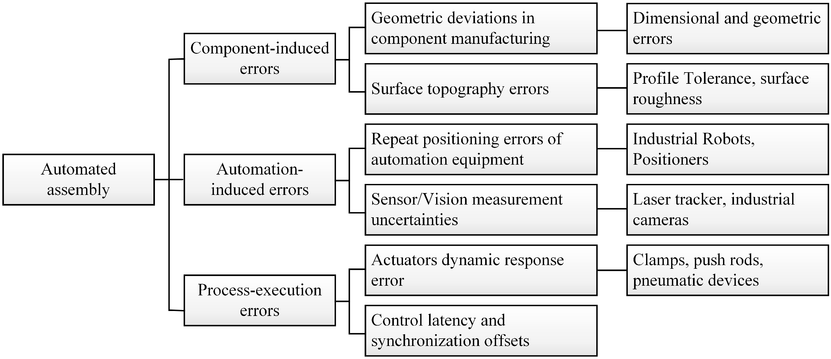
In automated assembly environments, part errors extend beyond traditional manufacturing tolerances to include novel deviations introduced by automated equipment and process execution. To systematically capture these multi-source errors, this study categorizes them into three classes: component-induced errors, automation-induced errors, and process-execution errors, as illustrated in Figure 3.
Critical error terms require mathematical formalization and parameterization to establish explicit model inputs for tolerance analysis and optimization prior to constructing multi-source error coupling models. This section defines mathematical representations and distribution patterns for distinct error types.

2.1.1. Component-Induced Errors

Part geometric deviations originate from the manufacturing stage, including dimensional errors and form errors caused by processes such as computer numerical control machining, stamping or additive manufacturing [31], and profiles or roughness caused by surface machining and grinding processes that do not meet design requirements [32]. These errors are usually obtained by sampling key geometric features of parts using a three-dimensional coordinate measurement system and comparing them with theoretical models to obtain deviations. Typical evaluation methods include statistical analysis of dimensional deviations, calculation of surface roughness power spectral density, and statistical regression analysis of material test samples [33].
  • Manufacturing geometric deviation
Component geometric deviations represent discrepancies between manufactured features and CAD models, typically expressed as vector differences between measured points and nominal surfaces. Let d i m e a s and d i n o m denote the measured and nominal coordinates of the i-th sampling point respectively. Then the manufacturing geometric deviation can be written as Equation (1).
δ d i = d i m e a s d i n o m
The collective deviation follows a normal distribution N μ d , σ d 2 , where μ d and σ d 2 represent the mean and standard deviation of sampled deviations [34,35].
2.
Surface topography errors
Surface topography is quantified using arithmetic average roughness R a , as shown in Equation (2).
R a = 1 L 0 1 z x d x
where z ( x ) denotes profile deviation from the mean line and L the evaluation length. Statistically, R a values follow a log-normal distribution L o g N μ r , σ r 2 [36].

2.1.2. Automation-System Errors

Automation-system errors arise from inherent characteristics of robotic equipment, actuators, and measurement systems. Robotic manipulators exhibit repeatability drift influenced by joint clearances and control system precision, with displacement ranges determined through repetitive positioning experiments [37]. Vision and laser measurement systems contain both systematic offsets and stochastic noise components, quantifiable using ISO-specified uncertainty evaluation protocols for coordinate measuring systems [38].
  • Repeat positioning error
The repeatability error of automated equipment is obtained by performing multiple positioning experiments on the same target. Assuming that the translation error between the end position and the reference position of the i-th experiment is Δ p i , and the rotation error is Δ θ i , the repeatability error can be described by the statistical distribution of these two sets of data, usually using a normal distribution, that is, Δ p N 0 , σ p 2 , Δ θ N 0 , σ p 2 . This mathematization provides the initial conditions for the device-level error in the coupling network.
2.
Sensor/vision measurement uncertainties
Sensor uncertainties combine systematic bias and random noise [39]. If y ˜ is the measured value and y is the true value, then it can be written as Equation (3).
y ˜ = y + b + ϵ
where b is the systematic deviation and ϵ is the zero-mean normal noise. Parameterizing this error allows the coupled model to distinguish between correctable errors and random perturbations and to assign tolerances accordingly in the optimization.

2.1.3. Process-Execution Errors

Distinct from manual assembly errors, automated assembly systems exhibit programmatically induced temporal and synchronization errors. Control latency manifests as statistically distributed time delays between command signals and physical responses, measurable through command–response timestamp analysis. Multi-axis and multi-robot operations demonstrate spatial–temporal misalignment during coordinated motion sequences, quantifiable through a synchronization log analysis of actuator initiation/termination timestamps. These temporal errors directly impact process sequence integrity and component fitment accuracy, necessitating compensation through time-series analysis and synchronization correction algorithms [40,41].
  • Actuator dynamic response error
End-effector dynamic errors manifest as force–displacement hysteresis during loading–unloading cycles. For applied force F and displacement δ , the hysteresis loop is modeled by δ F ; its hysteresis curve can be fitted by piecewise linear or polynomial function and combined with the damping coefficient c to represent the energy dissipation [41].
2.
Control latency and synchronization offsets
Sequence control delay τ refers to the time difference between command issuance and execution response [42]; multi-axis synchronization offset Δ t i j refers to the start/stop time difference of different execution units under the same instruction [43]. Both usually present log-normal distribution L o g N μ τ , σ τ 2 and normal distribution N 0 , σ Δ t 2 .

2.2. Multi-Source Error Coupling Modeling

Table 1 shows the error sources in automated assembly, which provides a clear input source for the subsequent error transmission chain model and a quantitative basis for error sensitivity analysis and weight allocation in multi-objective tolerance optimization.
In Table 1, all kinds of errors are discrete and do not have the prerequisite of linear superposition in the same coordinate system, so the traditional linear accumulation method of dimensional chain cannot be directly used. Errors such as manufacturing geometric deviation, positioning drift of automation equipment, and program control delay present different dimensions and distribution characteristics in space. If they are linearly accumulated, not only will the cross-coupling effect between errors be ignored, but it will also be difficult to reflect the actual situation of error amplification or offset. In order to accurately describe the error propagation and cumulative effects, it is necessary to first model the three types of errors separately, then build a coupling network at the key nodes of the assembly process and recursively propagate them.

2.2.1. Multi-Source Error Modeling

  • Component-induced error modeling
Let the i-th component-induced errors Δ M i be confined to the tolerance interval T i / 2 , + T i / 2 and assume a truncated normal distribution, then the geometric deviation can be expressed as Equation (4).
Δ M i N t r u n c ( 0 , σ G i 2 ; T i / 2 , + T i / 2 )
Using the Jacobian matrix J G , map each Δ M i into an assembly pose error Δ p c o m p , as shown in Equation (5).
Δ p c o m p = J G [ Δ M 1 , Δ M 2 , , Δ M n ] T
2.
Automation-system error modeling
The robot repetitive positioning error and measurement error are uniformly regarded as automation factor errors. The end linear error and angular error of the industrial robot can be approximately described by truncated normal distribution and mixed distribution respectively. The end linear position error of the robot is Δ L = ( Δ x , Δ y , Δ z ) T , and its distribution model is shown as Equation (6).
Δ L N t r u n c ( 0 , σ L 2 I 3 ; L max , + L max )
where I 3 denotes the 3 × 3 identity matrix, ensuring isotropic error distribution across all three spatial dimensions.
As multiple independent factors (e.g., servo resolution, kinematic compliance, sensor quantization) contribute to the robot’s positioning uncertainty, their aggregate effect is well approximated by a normal distribution according to the central limit theorem. Moreover, empirical studies of industrial robots have observed that repeatability errors (e.g., joint position deviations) follow a Gaussian pattern [44]. Therefore, we assume a zero-mean normal distribution for the robot’s repeatability error. We truncate this distribution at ± L max (the manufacturer-specified maximum positional error) to enforce the physical bound on extreme errors, ensuring no simulated error exceeds the robot’s known repeatability limits [45].
The end angle deviation Δ θ = ( Δ α , Δ β , Δ γ ) T then it approximately obeys a mixture of normal and uniform distribution, as shown in Equation (7).
Δ θ j w 1 N ( 0 , σ θ 2 ) + w 2 · U ( θ max , + θ max ) , j = 1 , 2 , 3
where w 1 + w 2 = 1 , θ max and L max are obtained according to the equipment manual and experimental calibration.
The robot’s orientation error is bounded (cannot exceed ± θ max by design) and yet can be unpredictably anywhere within that range. To capture this bounded yet random behavior, we model the angular error as a mixture of a Gaussian component and a uniform component. The zero-mean Gaussian part represents the typically small, frequent deviations about the commanded angle (due to controller precision and encoder noise), whereas the uniform part accounts for any larger bias or free-play within ± θ max (e.g., due to gear backlash or calibration drift) that could cause an arbitrary offset in orientation [46]. This mixed distribution ensures that most error instances are clustered around zero, as expected for a high-precision robot, while still allowing the errors to be distributed with moderate probability throughout the allowed range, which reflects the non-Gaussian orientation error behavior observed in practice.
The measurement error of the visual measurement system for posture can be divided into position measurement error Δ M p and attitude measurement error Δ M o . The position error is described by uniform distribution superimposed on normal distribution, as in Equation (8).
Δ M p u ( u m , u m ) + N ( 0 , σ m 2 I 3 ) , Δ M o N t r u n c ( 0 , σ o 2 I 3 ; θ o , θ o )
The chosen distributions for measurement errors reflect sensor characteristics and physical constraints. The position measurement error Δ M p is modeled as a uniform distribution (range ± u m ) superimposed on a normal distribution N ( 0 , σ m 2 ) . The uniform term represents a bounded systematic offset or quantization uncertainty (for instance, due to finite camera pixel resolution or an unknown calibration bias, assumed equally likely anywhere in ± u m ), while the Gaussian term captures random noise in the sensor measurement around the true value [47]. Meanwhile, the orientation measurement error Δ M o is assumed to follow a truncated normal distribution N trunc ( 0 , σ o 2 ; θ o , + θ o ) , reflecting that angular sensing errors are approximately Gaussian in distribution but cannot exceed a maximum angle θ o . In practice, the vision system’s field-of-view and algorithm impose hard limits on detectable orientation error; by truncating at ± θ o , we account for the physical limit beyond which the sensor would not provide a valid reading [48]. These distribution models thus incorporate realistic sensor noise profiles while respecting known bounds of the measurement system.
When the robot performs closed-loop correction under vision guidance, the terminal output deviation can be approximately written as Equation (9).
Δ p a u t o = J R Δ θ + K v Δ M p Δ M o
where J R is the robot Jacobian matrix, Δ θ is the joint angle error vector, and K v is the visual measurement mapping coefficient matrix. The statistical distribution of Δ p a u t o is obtained through Monte Carlo sampling, which provides a data basis for the “automation factor error input” of each node in the subsequent coupling network.
3.
Process-execution error modeling
Process-execution errors are mainly caused by the dynamic response of end-effectors such as clamps or actuators during load–unload cycles. This manifests as a force–displacement hysteresis effect. Let the applied normal force be F, and the resulting displacement be δ F . The loading–unloading path forms a closed-loop hysteresis curve, which can be represented by a piecewise polynomial model as shown in Equation (10).
δ F = a 1 F + b 1 + c 1 F ˙ , Loading branch a 2 F + b 2 + c 2 F ˙ , Unloading branch
where F ˙ is the rate of force application, and the coefficients a i , b i , c i capture the stiffness, preload offset, and damping-related energy loss, respectively. The system damping ratio ζ can be expressed via a viscous damping coefficient c, and the estimation method is shown in Equation (11).
ζ = c 2 k m
where k is the effective stiffness of the contact interface, and m is the equivalent mass of the actuator–part system. The net displacement deviation (Equation (12)) due to hysteresis is thus defined as the maximum deviation between loading and unloading paths at a given force level:
Δ δ δ l o a d F δ u n l o a d F
This residual deviation contributes to positional assembly error in the direction of the contact normal, and is mapped into the 6-DOF assembly error space via a transformation matrix T p .
Δ p proc = T p · Δ s x Δ s y Δ s z 0 0 0
Equation (13) preserves the physically observed nonlinear, rate-dependent, and asymmetric behaviors of tool–part interaction, ensuring that the process-induced positional errors are realistically captured and accurately integrated into the downstream error coupling model.

2.2.2. Multi-Source Error Coupling Network

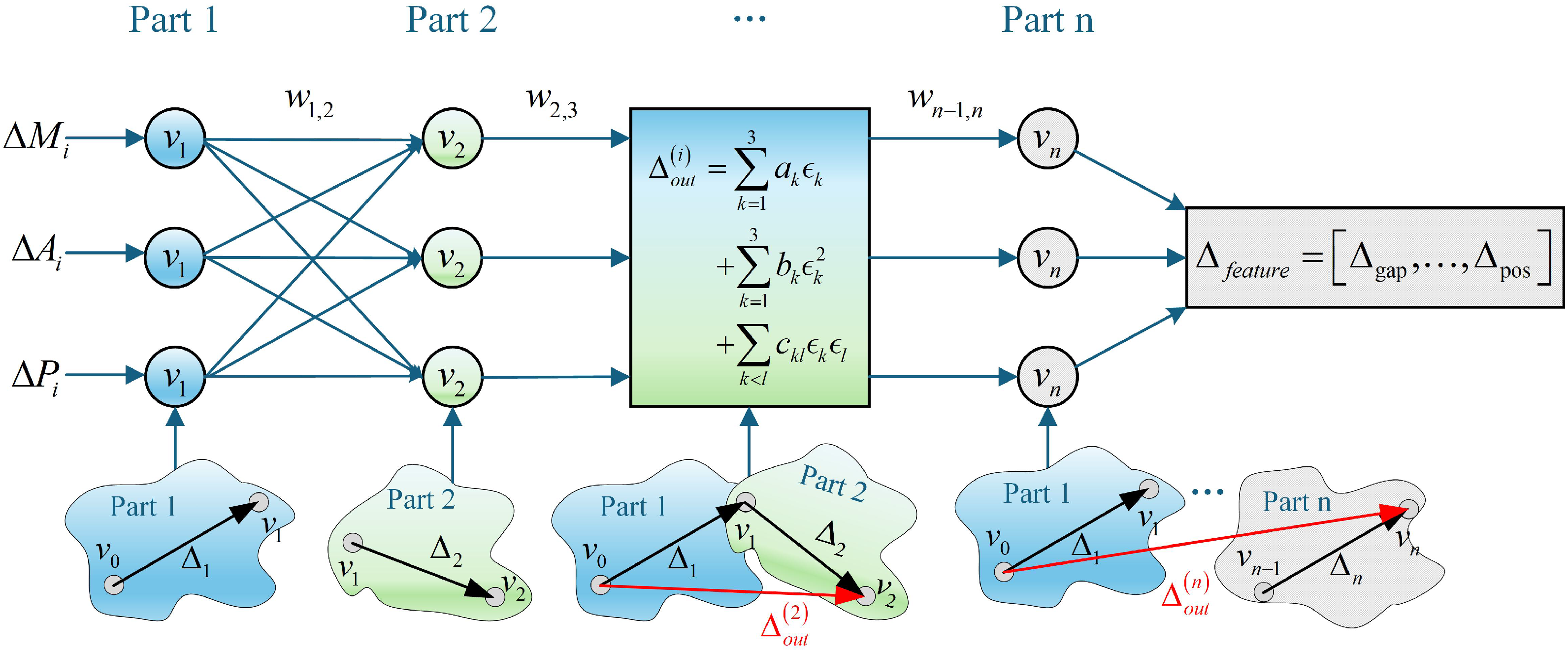
To capture the adjacency-aware propagation of multi-source errors, we define a coupling network model as shown in Figure 4. Each part introduces three types of errors: manufacturing ( Δ M ), alignment ( Δ A ), and process execution ( Δ P ). These errors propagate through inter-part adjacency weights to produce overall assembly deviations. The model incorporates not only linear and quadratic terms but also cross-coupling interactions among distinct error sources, as shown in Equation (14). The index l in the term k < l denotes the second variable in a distinct error pair, ensuring each cross-term ϵ k ϵ l is counted once. This structure reflects the directed graph in Figure 4, where nodes represent error inputs and links represent weighted coupling relations.
The notations in the figure above are defined as follows:
  • Δ M i : Component-induced errors;
  • Δ A i : Automation-related pose errors (including robot and sensing);
  • Δ P i : Process-execution errors from operations.
Each step of the assembly process is mapped to a network node v i in sequence. Each directed edge e i j represents the error transmission direction from node v i to the subsequent node v j and is assigned a weight w i j 0 , 1 to quantify the impact of the upstream error on the downstream step. At node v i , a semi-parametric polynomial coupling function F v i is defined to map the three types of input errors to output deviations, as shown in Equation (14).
Δ o u t i = k = 1 3 a k ϵ k + k = 1 3 b k ϵ k 2 + k < l c k l ϵ k ϵ l
where ϵ Δ M i , Δ A i , Δ P i ; a i is the linear sensitivity coefficient, reflecting the primary contribution of each single-error source to the current node; b i is the secondary amplification coefficient, which is used to describe the error accumulation or nonlinear growth effect; and c i is the cross-coupling coefficient, which is used to characterize the interaction or amplification effect between different error sources, such as the additional deviation generated when the geometric deviation and the actuator residual displacement interact with each other. On this basis, along each assembly path p = v 0 v 1 v n , the error recursive transmission can be expressed by Equation (15).
Δ p = F v n F v n 1 F v 1 Δ v 0
For each key matching feature, what is finally obtained is an error vector, whose components correspond to different quality indicators in turn, such as gap deviation, position deviation, etc., as shown in Equation (16).
Δ f e a t u r e = Δ g a p , Δ p o s ,
where Δ f e a t u r e is the final error vector. Each characteristic component is predicted and checked separately to ensure that each component meets the corresponding tolerance threshold E j * , as shown in Equation (17).
Δ f e a t u r e E j * , j = 1 , 2 , , m
The coupled network model system integrates the statistical characteristics and nonlinear cross-effects of three types of error sources, clarifies the error transmission path and amplification mechanism along the assembly process, and provides a rigorous mathematical foundation for feature-level precision control. Subsequent multi-objective tolerance optimization can obtain the quantitative impact of each tolerance parameter on the deviation of different assembly features based on this model, so as to allocate tolerances while meeting all precision thresholds. This model also supports critical path identification, which is used to determine the error node that has the greatest impact on the final assembly accuracy, providing a basis for subsequent process improvements or equipment calibration.

3. Multi-Objective Tolerance Optimization

3.1. Uncertainty Analysis and Optimization Model Construction

The multi-objective tolerance optimization is founded on a multi-source coupling model that captures how individual part tolerances propagate to assembly errors. In this framework, each geometric quality metric is expressed as a function of the relevant tolerances. These relationships are formally stated in Equations (14)–(17), which define the objective functions and constraints in terms of the coupled variation model; the optimization problem is formulated as Equation (18).
min θ Δ f e a t u r e ( θ ) = [ Δ g a p , Δ p o s i t i o n , ] s . t . θ i min θ i θ i max , i = 1 , , n
where θ = [ θ 1 , θ 2 , , θ n ] T represents the vector of tolerance parameters to be optimized, and Δ f e a t u r e ( θ ) are the feature deviations derived from the multi-source coupling network.
To account for the uncertainty in the automated assembly process, a Monte Carlo simulation of the assembly process is performed. Random samples are drawn from a specified distribution of part tolerances, and each sample is propagated through the coupled model to calculate the resulting feature deviations. Monte Carlo simulation is well suited for nonlinear tolerance analysis because it generates statistical samples of assembly responses by evaluating the response function for many random inputs. The Monte Carlo process is as follows:
  • Sample generation: Randomly generate sets of part dimensions according to their tolerance distributions;
  • Assembly evaluation: For each sample, apply the multi-source coupling model to compute the assembly feature deviations such as gap, coaxiality, etc.;
  • Statistical estimation: Compute performance metrics such as the mean and standard deviation of each error from the ensemble of simulated samples.
These simulated statistics serve as the basis for the optimization. The Monte Carlo outputs populate the objective functions in Equation (18), ensuring that the optimization model accounts for the actual distribution of each error under the given tolerances.

3.2. Sensitivity-Guided Multi-Objective Optimization via NSGA-II

To efficiently manage the complexity of the tolerance optimization problem, a global sensitivity analysis based on Sobol indices is conducted to identify the most influential tolerance parameters. The Sobol index for each input quantifies the proportion of output variance attributable to that parameter alone [49], as computed by Equation (19).
S T i = V a r θ i ( E [ Δ f e a t u r e | θ i ] ) V a r ( Δ f e a t u r e )
where S T i represents the total Sobol sensitivity index for the i-th tolerance parameter θ i ; Δ f e a t u r e represents the vector of assembly deviation metrics such as Δ g a p , Δ p o s i t i o n , etc.; V a r θ i ( E [ Δ f e a t u r e | θ i ] ) is the variance of the conditional expectation of feature deviations, given θ i ; and V a r ( Δ f e a t u r e ) is the total variance of the deviations.
Tolerance parameters with negligible Sobol indices are fixed at their nominal values to reduce the dimensionality of the optimization problem. With this reduced set of decision variables, the NSGA-II [22] is used for multi-objective tolerance optimization [50]. NSGA-II is a fast and elitist multi-objective genetic algorithm known for its good balance of convergence speed and diversity maintenance. It has been widely validated on engineering problems similar to ours. In particular, NSGA-II’s non-dominated sorting and crowding-distance mechanisms ensure a well-spread Pareto front, which is crucial for exploring trade-offs between positional accuracy and coaxiality in our case.
The NSGA-II algorithm operates as follows:
  • Initialization: An initial population is generated by assigning random values to each retained tolerance parameter within their allowable ranges;
  • Evaluation: For each candidate solution, the corresponding geometric deviations are computed using the Monte Carlo-based coupling model;
  • Non-dominated sorting: All solutions are ranked into Pareto fronts based on dominance relations;
  • Selection and genetic operations: Tournament selection, crossover, and mutation operators are applied to create offspring;
  • Iteration: The evaluation and sorting process is repeated over multiple generations until convergence is achieved.
This approach yields a Pareto-optimal set of tolerance configurations, each representing a unique trade-off among geometric deviation objectives [51]. For example, one configuration might minimize one deviation at the expense of another, while another configuration achieves balanced control across all metrics. These trade-offs provide a basis for selecting tolerance schemes that best align with design priorities.

3.3. Optimization Procedure Flowchart

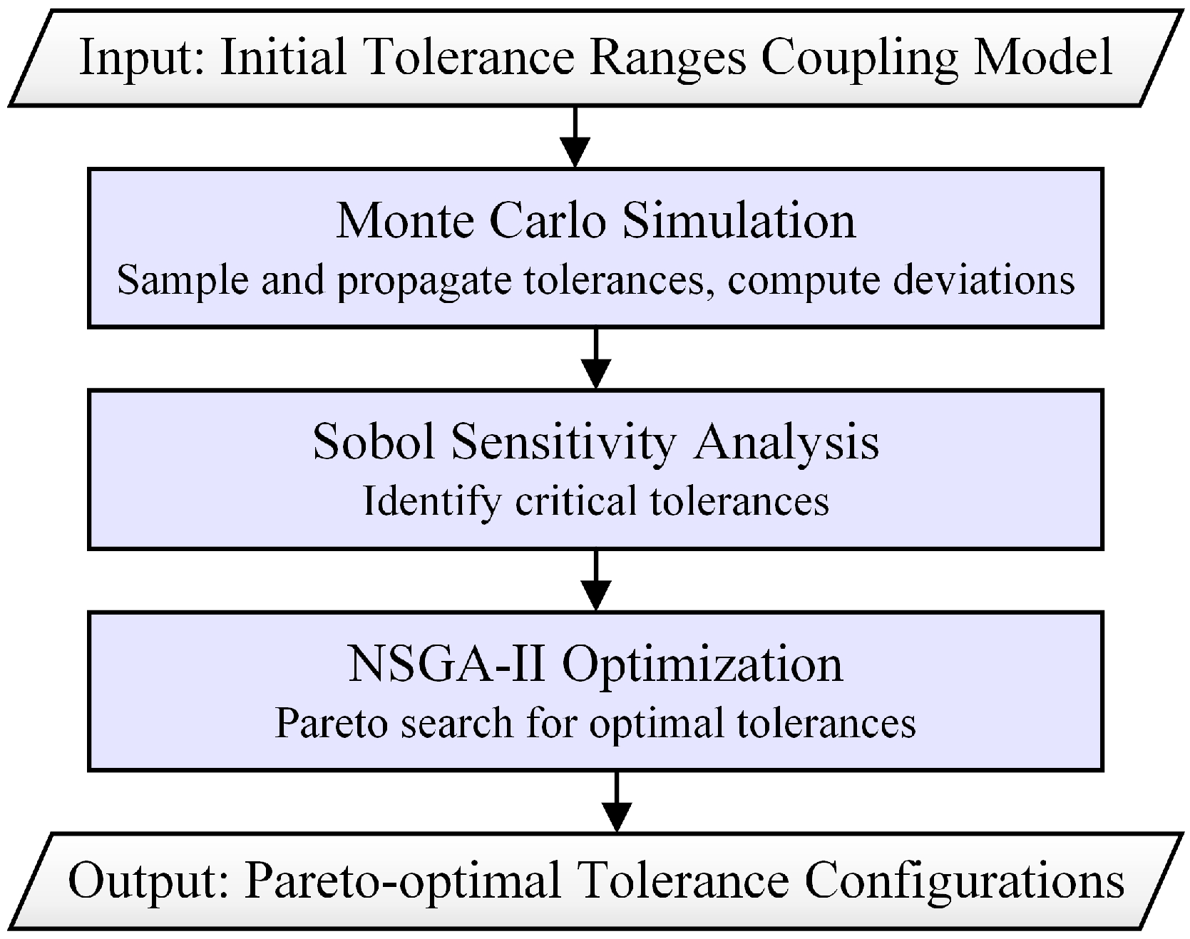
Figure 5 illustrates the complete workflow of the proposed tolerance optimization methodology, integrating multi-source uncertainty simulation, sensitivity analysis, and evolutionary optimization. The process begins with the input of initial tolerance ranges, which are modeled using the previously defined multi-source coupling network to characterize how geometric and process errors propagate through the assembly system.
The steps are detailed below:
  • In the first step, a Monte Carlo simulation is conducted. This stage repeatedly samples tolerance values based on the defined uncertainty ranges and propagates them through the coupling model. By computing the resulting deviation distributions (e.g., for position and coaxiality), this step provides a statistical foundation for evaluating how tolerances impact assembly quality.
  • In the second step, a Sobol sensitivity analysis is applied to the simulation results. This variance-based method quantifies the contribution of each tolerance variable to the variation in key performance indicators. By identifying the most influential tolerances, this step effectively reduces the dimensionality of the optimization problem, focusing efforts on parameters that matter most.
  • In the third step, the NSGA-II multi-objective evolutionary algorithm is employed to optimize the influential tolerance parameters. NSGA-II searches for a Pareto front of solutions that balance competing objectives (e.g., minimizing positional and coaxiality deviations) while ensuring feasibility and process robustness. The algorithm iteratively evolves candidate solutions by simulating selection, crossover, and mutation across generations, guided by dominance ranking and crowding distance.
Finally, the workflow yields a set of Pareto-optimal tolerance configurations. These configurations offer flexible trade-offs that can be selected based on specific manufacturing priorities, such as cost, precision, or yield. This integrated workflow ensures that the optimized tolerances are both practically viable and statistically robust, enabling improved assembly quality under realistic manufacturing conditions.

3.4. Optimization Scenarios

To evaluate the contribution of different sources of error to the final assembly quality, three distinct optimization scenarios are defined:
  • Component-only optimization: Only the tolerances related to the manufactured parts ( Δ M ) are included as decision variables in the optimization. All process and automation-related parameters ( Δ A , Δ P ) are kept constant at their nominal values.
  • Process-only optimization: Only the process-related factors, such as robotic positioning accuracy and process-execution errors ( Δ A and Δ P ), are optimized. Component tolerances remain fixed at their initial values.
  • Full optimization: All tolerance and error-related parameters ( Δ M , Δ A , and Δ P ) are optimized simultaneously to achieve the best overall assembly quality.
These three optimization modes allow for a comparative analysis to isolate the impact of each error source and assess the effectiveness of targeted improvement strategies.

4. Case Study: Automatic Assembly of Helicopter Rings

4.1. Case Overview and Setup

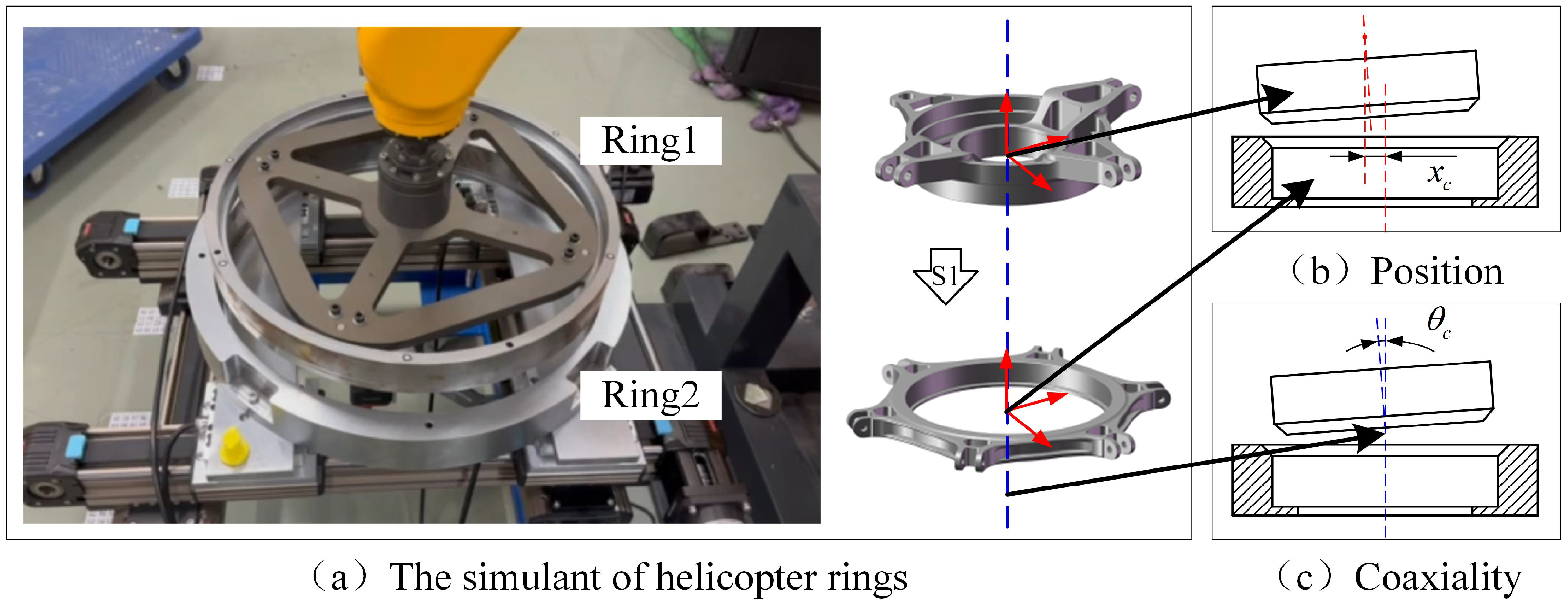
The automatic assembly of the helicopter rotor ring (tilt mechanism) is analyzed, and its tolerance scheme is optimized. The assembly consists of a moving ring and a fixed ring, and its key quality indicators are the position alignment of the ring center and the coaxiality of its axis. Figure 6 shows the assembly setup and assembly features.
Three types of error sources are defined on the mating surface to simulate assembly uncertainty:
  • Δ M for the geometric error caused by the two rings and the end fixture, initially defined as ±0.2 mm;
  • Δ A for the positioning error of the industrial robot, defined as ±0.12 mm, ±0.01°, which can be found in Appendix A;
  • Δ P for the jitter error caused by the gripper during the pick-and-place process, initially defined as ±0.3 mm.
Each error is applied to the corresponding mating surface in order to analyze its impact on the assembly alignment. And two key quality metrics are monitored:
  • Δ p o s i t i o n for the positional deviation between the centers of the rings;
  • Δ c o a x i a l i t y for the angular deviation between the center axes of the rings.
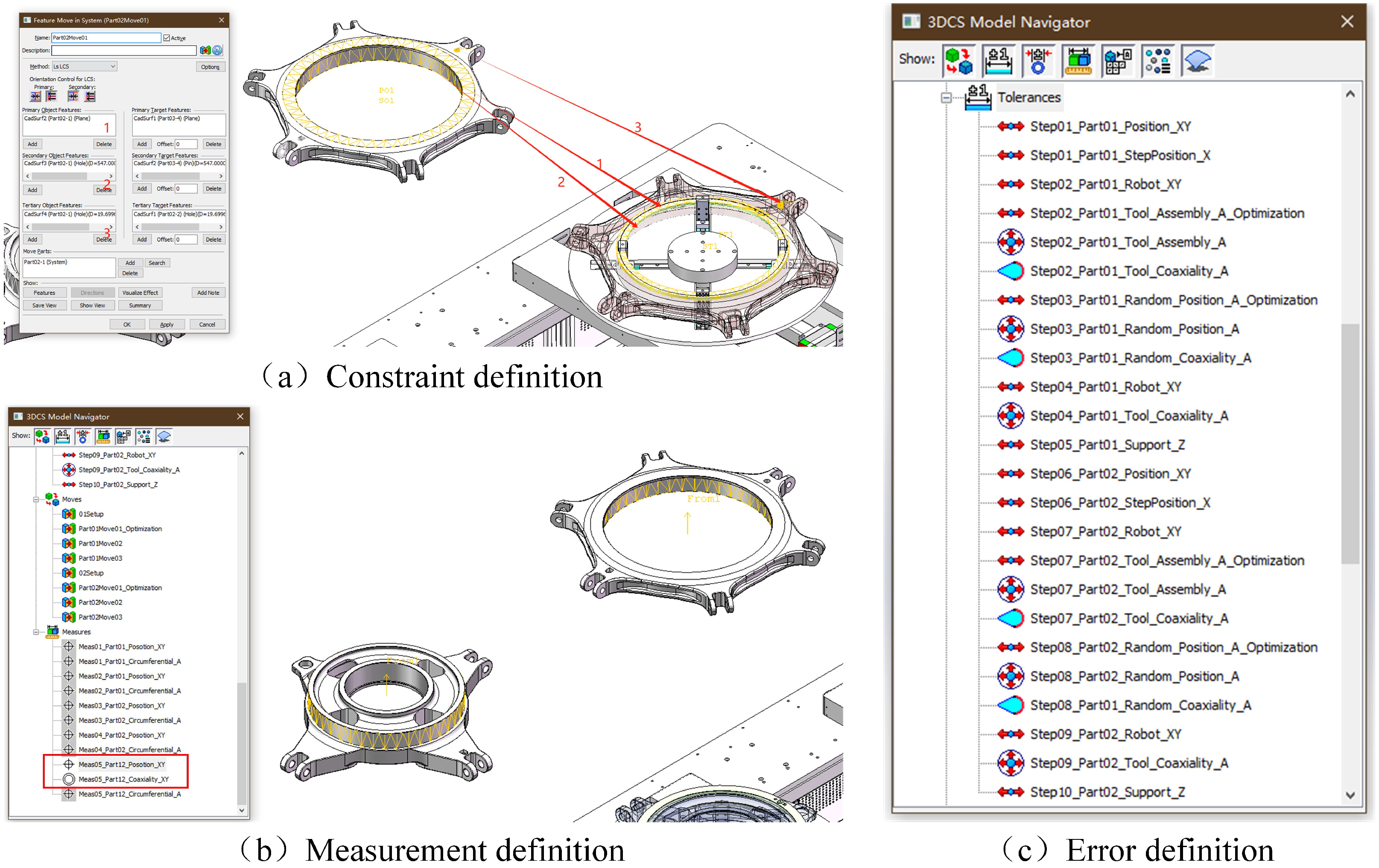
The realization of the fit constraints between the rings and the definition of the above errors and measurements of key quality metrics are achieved with the help of the tolerance analysis software 3DCS Variation Analyst for SOLIDWORKS (x64) Version 7.7.0.1. [52], as shown in Figure 7.
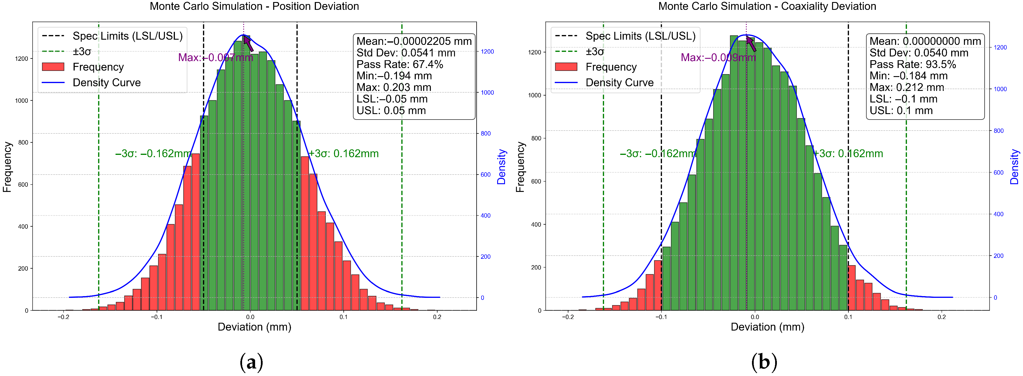
Monte Carlo simulations were performed to propagate uncertainty. For each output metric, 20,000 trials were conducted; Δ M , Δ A , and Δ P were randomly drawn within their range; and the resulting deviations were calculated. Figure 8 summarizes the results. To visualize the statistical distribution of assembly deviations obtained through Monte Carlo simulations, the frequency histograms in Figure 8 and Figure 9 were constructed using the following binning method, as shown in Equation (20).
f i = n i n · w , i = 1 , 2 , , k
where f i denotes the frequency (density) value of the i-th bin, n i is the number of deviation samples falling within the i-th bin interval, n is the total number of samples generated from the Monte Carlo simulation, and w is the bin width. The density curve overlaid in the plots was estimated using Gaussian kernel density estimation (KDE) for better visualization of distribution shapes.
CPK is a widely used statistical metric in manufacturing that is employed here to evaluate the assembly quality of positional and coaxiality deviations. CPK is calculated as Equation (21):
C P K = min U S L μ 3 σ , μ L S L 3 σ
where μ is the process mean, σ is the standard deviation obtained from Monte Carlo simulation, and U S L and L S L represent the upper and lower specification limits defined by assembly tolerances.
The U S L and L S L for each assembly quality feature were determined according to relevant aerospace industry standards and customer requirements for tolerance control [53]. Where customer specifications were available, these values were adopted directly. For features without explicit customer-provided limits, industry standards for precision aerospace assembly were applied to define conservative yet practical bounds. This ensures that the capability assessment is directly aligned with real-world production constraints.
CPK follows widely accepted benchmarks in manufacturing quality control, and a higher CPK indicates a more capable process [54,55]. The differences are detailed below:
  • CPK 1.33 : The process capability is considered good, meaning it can stably and consistently produce products within specifications.
  • 1.00 CPK < 1.33 : The process capability is moderate, indicating that while products generally meet specifications, continuous monitoring and improvement are required to maintain quality.
  • CPK < 1.00 : The process capability is insufficient, suggesting that the process is unable to reliably produce within specifications and corrective actions are necessary.
In our analysis, these benchmarks were used to contextualize the optimization results. For example, a CPK value of 1.11 indicates a capable process that meets specifications but leaves less margin than the “excellent” threshold, guiding further process refinement.
As shown in Figure 8, these results highlight that geometric variation ( Δ M ) and gripper jitter ( Δ P ) can cause significant misalignment, especially for the tight positional tolerance. Thus, a three-stage framework (Figure 5) is used for tolerance optimization:
Step 1:
Monte Carlo Uncertainty Propagation: The initial simulation quantified the combined effect of all error sources on the assembly deviations, as shown in Figure 8.
Step 2:
Global Sensitivity Analysis: The total Sobol index of each error source is calculated to distribute the output variance. The results show that Δ M contributes ~86.4% of the variance, Δ P ~12.8%, and Δ A only ~0.8%. This confirms that geometric variation is the dominant source, gripper jitter is secondary, and robot error is negligible. Consequently, Δ A is fixed at its nominal tolerance in the optimization to reduce complexity.
Step 3:
Multi-Objective Tolerance Optimization: The remaining tolerances Δ M and Δ P are optimized using NSGA-II. The goal was to minimize the combined standard deviation of Δ p o s i t i o n and Δ c o a x i a l i t y while improving CPK. Each candidate tolerance set was evaluated through 20,000 Monte Carlo runs to assess its performance. The algorithm identified the Pareto frontier of solutions that traded off between tight tolerances and achievable variability.
From the Pareto optimal frontier, a representative “inflection point” solution is selected to best balance assembly accuracy and manufacturing feasibility. This solution yields the following updated tolerances:
  • Δ M : Tightened from the initial ±0.20 mm to ±0.15 mm;
  • Δ A : Retained at ±0.12 mm and ±0.01°, due to its negligible influence (Sobol contribution < 1%);
  • Δ P : Tightened from ±0.30 mm to ±0.12 mm.
These adjustments conform to the Sobol ordering, focusing tolerance adjustments on the most influential error sources. The optimization scheme is then validated through subsequent Monte Carlo simulations.

4.2. Comparison of Optimization Strategies

To understand the effectiveness of different optimization approaches, we compare the results of component-only, process-only, and full optimization strategies. Each strategy uses the same multi-objective optimization framework, but with different sets of active decision variables:
  • In the component-only strategy, only component-related tolerances ( Δ M ) are adjusted, such as machining or manufacturing precision of parts.
  • The process-only strategy focuses on reducing automation and execution errors ( Δ A , Δ P ), such as robotic positioning deviations and gripper jitter, while holding part tolerances constant.
  • The full optimization strategy jointly considers all types of errors for a comprehensive improvement.
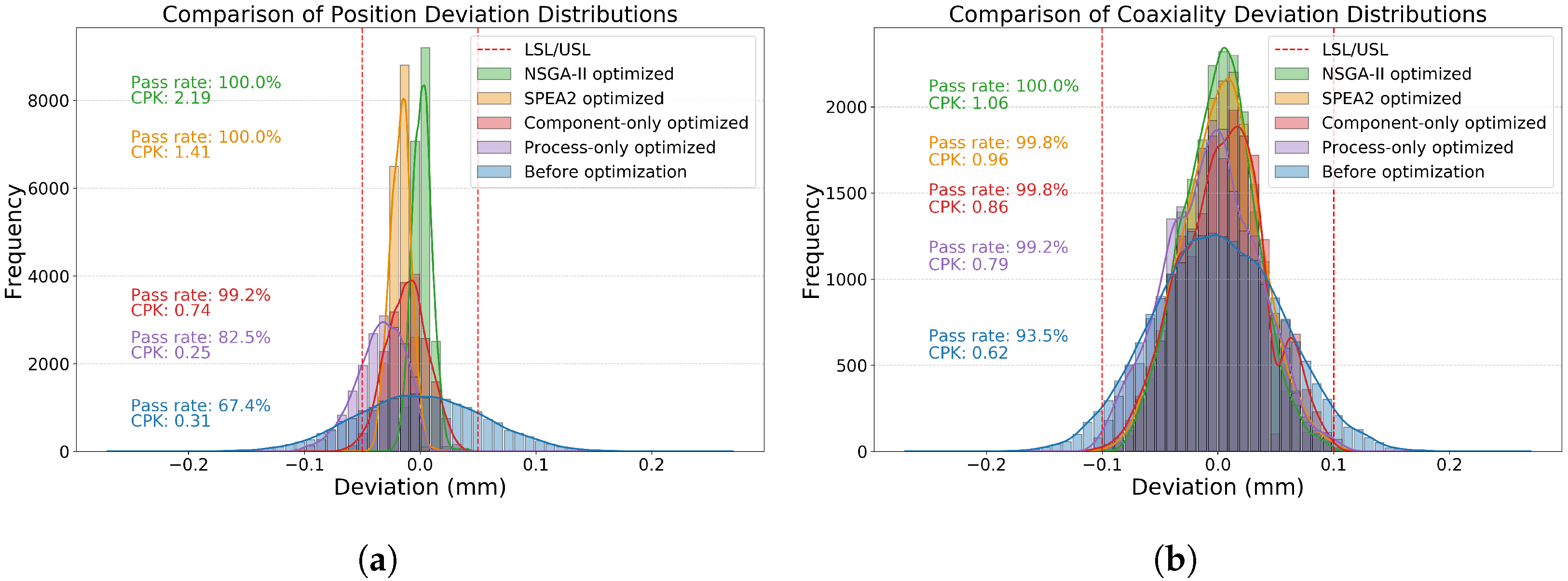
This classification allows for a fair evaluation of how much improvement can be achieved by targeting specific error sources. The resulting deviations and process capability indices (CPK) are shown in Figure 9, where each bar or curve corresponds to one of these four strategies.
In addition to the NSGA-II optimization method described in this article, we also performed comparative optimization using the Strength Pareto Evolutionary Algorithm 2 (SPEA2). SPEA2 shares the multi-objective evolutionary framework [56]. While SPEA2 employs a different fitness assignment and archive truncation strategy than NSGA-II [57], it is also widely used for multi-objective optimization. In our case, it serves as a comparative benchmark to assess the robustness and balance of NSGA-II’s solutions.

4.3. Optimization Results and Discussion

Figure 9 demonstrates the effectiveness of the NSGA-II-based multi-objective tolerance optimization in reducing positional and coaxiality deviations in the ring assembly process. As shown in Figure 9a, for positional deviation, the original tolerance scheme results in a broad spread and significant skewness, yielding a pass rate of only 67.4% and a CPK of 0.31. After applying the NSGA-II optimization, the distribution becomes sharply concentrated around the target, resulting in a pass rate of 100.0% and a CPK of 2.19, indicating excellent process capability. The SPEA2-optimized result achieves the same pass rate of 100.0%, with a slightly lower CPK of 1.41, suggesting slightly reduced robustness compared to NSGA-II. Component-only and process-only optimization schemes achieve pass rates of 99.2% and 82.5%, with CPK of 0.74 and 0.25, respectively. In Figure 9b, coaxiality deviation also shows clear improvements. The original process yields a pass rate of 93.5% and a CPK of 0.62. NSGA-II optimization raises the pass rate to 100.0% and improves the CPK to 1.06. SPEA2 optimization achieves a comparable pass rate of 99.8% and a CPK of 0.96. Component-only and process-only optimizations both yield pass rates of 99.8% and 99.2%, but with CPK of 0.86 and 0.79, respectively. These results confirm that NSGA-II provides the most balanced improvement across both quality indicators.
In our setting, the post-screening decision space is low-dimensional, and the feasible trade-off between position and coaxiality is narrow with a distinct knee. NSGA-II’s elitist non-dominated sorting on the combined parent–offspring population, followed by crowding-distance selection, preserves boundary and knee solutions and maintains a uniform spread along the front. Under Monte Carlo objective evaluations, the rank-then-crowding tournament used by NSGA-II is also less affected by small fitness fluctuations than the strength-based fitness and k-nearest-neighbor density estimator used in SPEA2, which can bias selection toward the center of the front. Consequently, NSGA-II converged more reliably to well-distributed boundary solutions, yielding slightly tighter deviation distributions and higher CPK values than SPEA2 in our experiments.

5. Discussion: Generalizability and Limitations

The proposed framework, which integrates multi-source error modeling, uncertainty propagation, and multi-objective tolerance optimization, is designed with adaptability in mind. While our case study focused on the assembly of coaxial helicopter rings, the underlying methodology is applicable to a broad range of complex assembly tasks across various industries. Our approach can be extended to assemblies involving different geometries and functional constraints, such as aircraft skin-to-frame panel assembly, automotive body-in-white processes, or spacecraft module alignment. The error propagation network (Section 2.2) can be adapted to model different contact sequences and component interactions. For example, flat panel assemblies may emphasize parallelism and flushness, while shaft-bearing fits may focus more on concentricity and clearance. Moreover, the use of a directed graph-based coupling model allows the inclusion of hierarchical or dependent assembly steps, enabling scalable modeling even in large and interdependent assemblies. As long as the error sources—such as manufacturing variability, fixture misalignment, or robot positioning errors—can be measured or estimated, the methodology can be recalibrated for a new context.
Despite its generality, several practical limitations remain: (a) The accuracy of the model relies on the representativeness of error distribution assumptions. Different industrial contexts may involve non-Gaussian errors, dynamic disturbances, or material deformations not captured by our current formulation. (b) The computational load of Monte Carlo simulations increases with assembly size and complexity; efficient sampling strategies or surrogate models may be needed for real-time applications. (c) The model currently assumes a static assembly sequence; extensions to adaptive or feedback-based strategies could further enhance robustness.
Future work could explore the integration of real-time data from digital twins or in-line sensors to adaptively update the error models. Additionally, testing alternative evolutionary optimization strategies or machine learning-assisted decision models may improve performance in highly nonlinear or multi-objective trade-off spaces. Our framework lays the foundation for these extensions and can serve as a blueprint for intelligent tolerance control in smart manufacturing systems.

6. Conclusions

This paper presents an integrated methodology for multi-objective tolerance optimization under multi-source uncertainty in automated robotic assembly. Addressing the limitations of conventional tolerance analysis in nonlinear, data-driven manufacturing environments, the proposed approach introduces three key innovations:
  • A three-level uncertainty classification model that systematically captures geometric manufacturing deviations, robotic system positioning errors, and execution-induced process fluctuations;
  • A directed graph-based semi-parametric coupling network that models the dynamic propagation of deviations across sequential assembly operations, enabling accurate quality estimation via Monte Carlo simulation;
  • A tolerance optimization strategy that integrates Sobol-based global sensitivity analysis to identify dominant parameters with NSGA-II to explore Pareto-optimal tolerance configurations.
To verify the effectiveness of the proposed strategy, a representative coaxial ring assembly scenario was adopted. The results demonstrate significant quality improvement in both position and coaxiality metrics after optimization. For position deviation, the pass rate increased from 67.4% to 100.0%, and the CPK improved markedly from 0.31 to 2.19. For coaxiality deviation, the pass rate increased from 93.5% to 100.0%, and the CPK rose from 0.62 to 1.06. These results are detailed in Figure 8.
Comparative analysis with alternative optimization strategies (Figure 9) further underscores the robustness of our method: the NSGA-II-based scheme outperformed SPEA2, component-only, and process-only optimization strategies in both pass rate and CPK for all metrics. This highlights the importance of coordinated tolerance allocation and joint modeling under multi-source uncertainty.
Overall, this work demonstrates that the integration of sensitivity-guided optimization and dynamic deviation modeling provides a rigorous and effective pathway for tolerance synthesis in complex robotic assemblies. The proposed framework also provides a foundation for future integration into digital twin-based quality assurance systems and broader applications in intelligent manufacturing scenarios.

Author Contributions

Conceptualization, X.H.; methodology, S.L.; validation, G.H., T.C.; writing—original draft preparation, T.C.; writing—review and editing, T.C. All authors have read and agreed to the published version of the manuscript.

Funding

This research received no external funding.

Institutional Review Board Statement

Not applicable.

Informed Consent Statement

Not applicable.

Acknowledgments

The authors gratefully acknowledge the insightful comments by the editors and the anonymous referees. This work was partially supported by the Aircraft Assembly Laboratory (Nanjing University of Aeronautics and Astronautics).

Conflicts of Interest

The authors declare that they have no known competing financial interests or personal relationships that could have appeared to influence the work reported in this paper.

Abbreviations

The following abbreviations are used in this manuscript:
NSGA-IINon-dominated sorting genetic algorithm II
CPKProcess capability index
CADComputer-aided design
SPEA2Strength pareto evolutionary algorithm 2
RMSERoot mean square error

Appendix A. Experiment on the Repeatability of KUKA KR90 Robot
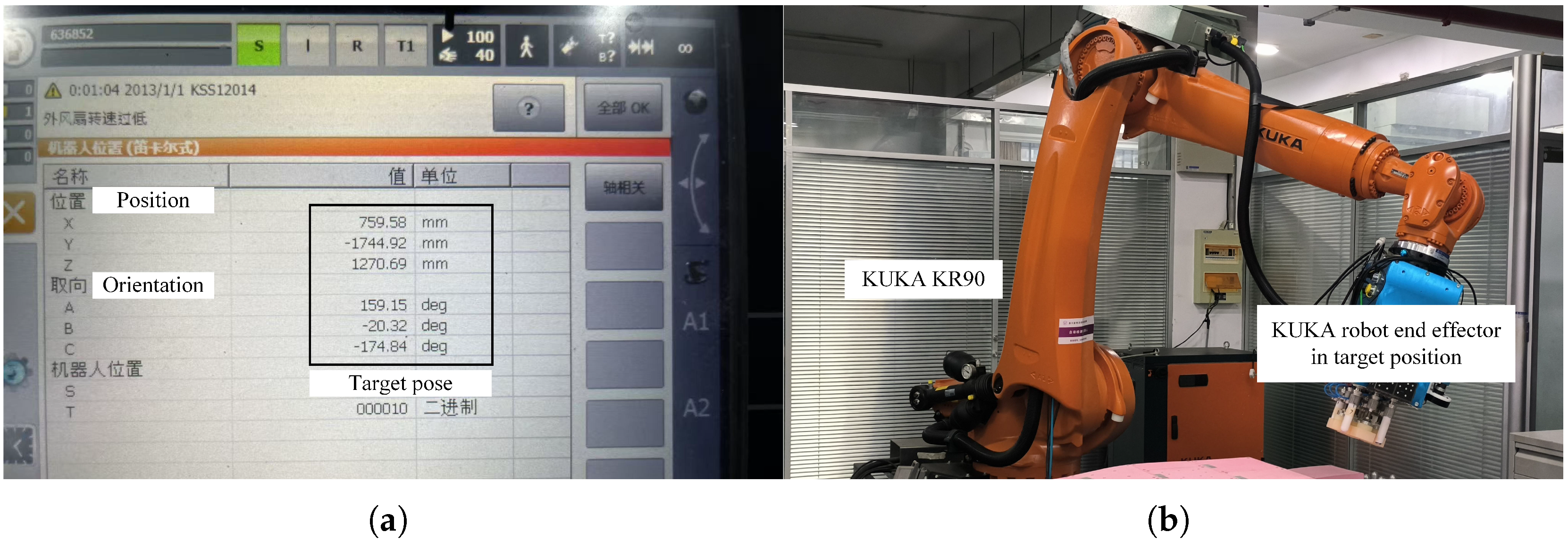
Figure A1 shows the target position of the robot in the experiment on the repeatability of the KUKA KR90 robot, as well as the posture under the target position.
Figure A1. KUKA KR 90 industrial robot repeat positioning accuracy test. (a) Target pose of the KUKA robot end-effector; (b) KUKA KR90 robot under the target pose.
Machines 13 00736 g0a1
Taking the KUKA KR90 model as an example, referring to the ISO 9283 [58] standard, the robot was repeatedly positioned under the same target posture to statistically analyze its error characteristics. Detailed experimental data are shown in Table A1. The experimental results show that the repeated positioning error is divided into linear error x and angular error α . Line error x represents the offset of the end position, and its root mean square error is about 0.12 mm. It is statistically close to a truncated normal distribution with a zero mean. Angular error α represents the deviation of the end posture. In multiple tests, it was found that the root mean square error of the angle was about 0.01°. The error distribution shows a mixed characteristic, which can be approximately expressed as a weighted combination of normal distribution and uniform distribution.
Table A1. KUKA KR90 robot repeat positioning accuracy test data.
Numx
(mm)
y
(mm)
z
(mm)
α
(°)
β
(°)
γ
(°)
Linear
(mm)
Angular
(°)
Target759.58−1744.921270.69159.15−20.32−174.84
1759.70−1744.911270.66159.16−20.31−174.840.12830.0085
2759.70−1744.931270.68159.16−20.31−174.830.11920.0119
3759.71−1744.931270.68159.15−20.31−174.830.12740.0144
4759.72−1744.911270.67159.16−20.31−174.830.13670.0128
5759.70−1744.901270.69159.16−20.32−174.840.11950.0060
6759.70−1744.901270.70159.15−20.32−174.840.11940.0051
7759.72−1744.941270.73159.16−20.31−174.830.14190.0153
8759.71−1744.931270.69159.16−20.31−174.840.12790.0096
9759.70−1744.911270.70159.15−20.31−174.830.11560.0092
10759.71−1744.901270.69159.16−20.30−174.830.12690.0194
11759.70−1744.931270.65159.15−20.31−174.840.12200.0074
12759.70−1744.921270.69159.16−20.31−174.840.11540.0122
13759.70−1744.941270.69159.16−20.31−174.840.12440.0125
14759.68−1744.941270.74159.15−20.31−174.840.11480.0076
15759.68−1744.901270.69159.16−20.32−174.840.10410.0098
16759.69−1744.921270.70159.16−20.31−174.840.11770.0097
17759.69−1744.921270.69159.16−20.32−174.830.10990.0127
18759.70−1744.901270.67159.16−20.32−174.840.12690.0115
19759.69−1744.911270.71159.15−20.32−174.840.11350.0067
20759.69−1744.931270.71159.15−20.31−174.830.10770.0080
21759.71−1744.911270.71159.15−20.31−174.830.13580.0153
22759.70−1744.891270.67159.15−20.32−174.840.12300.0027
23759.70−1744.921270.72159.15−20.31−174.830.12390.0120
24759.69−1744.891270.66159.16−20.32−174.830.11380.0078
25759.69−1744.971270.70159.16−20.32−174.840.12650.0071
26759.70−1744.901270.73159.16−20.31−174.830.12980.0128
27759.69−1744.921270.67159.16−20.31−174.830.11030.0091
28759.70−1744.931270.68159.16−20.32−174.840.12440.0100
29759.69−1744.921270.69159.15−20.32−174.830.11400.0073
30759.70−1744.961270.68159.16−20.31−174.840.12410.0154
31759.69−1744.921270.66159.16−20.32−174.830.11820.0091
32759.72−1744.911270.69159.15−20.31−174.830.13870.0093
33759.70−1744.891270.67159.15−20.31−174.830.12530.0112
34759.69−1744.931270.70159.16−20.32−174.840.11030.0072
35759.71−1744.941270.67159.15−20.31−174.830.13050.0167
36759.69−1744.931270.72159.16−20.31−174.840.11260.0100
37759.70−1744.901270.67159.16−20.32−174.840.12440.0079
38759.68−1744.911270.68159.15−20.31−174.830.10080.0100
39759.69−1744.931270.71159.15−20.32−174.830.10850.0070
40759.70−1744.911270.67159.15−20.31−174.840.12490.0082
41759.71−1744.921270.69159.15−20.32−174.840.12750.0063
42759.70−1744.901270.72159.16−20.32−174.840.12600.0096
43759.70−1744.931270.66159.16−20.31−174.840.12390.0092
44759.70−1744.931270.69159.15−20.31−174.830.11720.0108
45759.69−1744.931270.70159.16−20.32−174.830.10560.0083
46759.69−1744.951270.71159.16−20.32−174.840.11760.0079
47759.70−1744.911270.67159.15−20.32−174.830.11820.0088
48759.71−1744.911270.66159.16−20.32−174.830.13330.0086
49759.70−1744.921270.70159.16−20.31−174.830.12390.0137
50759.68−1744.921270.70159.15−20.31−174.830.10260.0094
RMSE 0.1210540.010466

References

  1. Webb, P.; Eastwood, S.; Jayweera, N.; Ye, C.; Keown, C.M. An Automated Fuselage Panel Assembly and Riveting Cell-Validation and Testing; Technical report, SAE Technical Paper; SAE: Warrendale, PA, USA, 2006. [Google Scholar]
  2. Bhatia, V.; Kumar, A.; Sidharth, S.; Khare, S.K.; Ghorpade, S.C.; Kumar, P.; AlZohbi, G. Industry 4.0 in Aircraft Manufacturing: Innovative Use Cases and Patent Landscape. In Industry 4.0 Driven Manufacturing Technologies; Springer: Berlin/Heidelberg, Germany, 2024; pp. 103–137. [Google Scholar]
  3. Buergin, J.; Helming, S.; Andreas, J.; Blaettchen, P.; Schweizer, Y.; Bitte, F.; Haefner, B.; Lanza, G. Local order scheduling for mixed-model assembly lines in the aircraft manufacturing industry. Prod. Eng. 2018, 12, 759–767. [Google Scholar] [CrossRef]
  4. Larsen, L.; Endrass, M.; Jarka, S.; Bauer, S.; Janek, M. Exploring ultrasonic and resistance welding for thermoplastic composite structures: Process development and application potential. Compos. Part B Eng. 2025, 289, 111927. [Google Scholar] [CrossRef]
  5. Mei, B.; Zhu, W. Accurate positioning of a drilling and riveting cell for aircraft assembly. Robot. Comput.-Integr. Manuf. 2021, 69, 102112. [Google Scholar] [CrossRef]
  6. Muelaner, J.; Martin, O.; Maropoulos, P. Achieving low cost and high quality aero structure assembly through integrated digital metrology systems. Procedia CIRP 2013, 7, 688–693. [Google Scholar] [CrossRef]
  7. Chen, C.; Sun, J.; Wang, L.; Chen, G.; Xu, M.; Ni, J.; Ramli, R.; Su, S.; Chu, C. Pneumatic bionic hand with rigid-flexible coupling structure. Materials 2022, 15, 1358. [Google Scholar] [CrossRef] [PubMed]
  8. Liu, X.; Wei, Y.; Qiu, Y. Advanced flexible skin-like pressure and strain sensors for human health monitoring. Micromachines 2021, 12, 695. [Google Scholar] [CrossRef]
  9. Dong, Y.; Hussain, I.; He, S. Structural topology optimization of aircraft wing leading edge fabricated of multilayer composites. Aerosp. Sci. Technol. 2025, 159, 109993. [Google Scholar] [CrossRef]
  10. Torres, Y.; Nadeau, S.; Landau, K. Classification and quantification of human error in manufacturing: A case study in complex manual assembly. Appl. Sci. 2021, 11, 749. [Google Scholar] [CrossRef]
  11. Jamshidi, J.; Kayani, A.; Iravani, P.; Maropoulos, P.G.; Summers, M. Manufacturing and assembly automation by integrated metrology systems for aircraft wing fabrication. Proc. Inst. Mech. Eng. Part B J. Eng. Manuf. 2010, 224, 25–36. [Google Scholar] [CrossRef]
  12. Klagesa, B.; Grafa, J.; Zaeha, M. Human errors in manual assembly—A survey on current and future relevance. Procedia CIRP 2024, 130, 1556–1561. [Google Scholar] [CrossRef]
  13. Slamani, M.; Nubiola, A.; Bonev, I. Assessment of the positioning performance of an industrial robot. Ind. Robot. Int. J. 2012, 39, 57–68. [Google Scholar] [CrossRef]
  14. Grohmann, P.; Walter, M.S. Speeding up Statistical Tolerance Analysis to Real Time. Appl. Sci. 2021, 11, 4207. [Google Scholar] [CrossRef]
  15. Sigron, P.; Aschwanden, I.; Bambach, M. Compensation of geometric, backlash, and thermal drift errors using a universal industrial robot model. IEEE Trans. Autom. Sci. Eng. 2023, 21, 6615–6627. [Google Scholar] [CrossRef]
  16. Bell, J.; Redmond, L.; Carpenter, K.; de la Croix, J.P. Numerical Simulation and Influence of Non-Gaussian Vibrations on Flexible Robotic Systems. J. Spacecr. Rocket. 2024, 61, 1084–1098. [Google Scholar] [CrossRef]
  17. Liu, X.; Zheng, L.; Wang, Y.; Yang, W.; Wang, B.; Liu, B. Assembly error modeling and tolerance dynamic allocation of large-scale space deployable mechanism toward service performance. Appl. Sci. 2023, 13, 4999. [Google Scholar] [CrossRef]
  18. Makulavičius, M.; Petkevičius, S.; Rožėnė, J.; Dzedzickis, A.; Bučinskas, V. Industrial robots in mechanical machining: Perspectives and limitations. Robotics 2023, 12, 160. [Google Scholar] [CrossRef]
  19. Nagarajan, L.; Mahalingam, S.K.; Salunkhe, S.; Nasr, E.A.; Davim, J.P.; Hussein, H.M. A novel methodology for simultaneous minimization of manufacturing objectives in tolerance allocation of complex assembly. Appl. Sci. 2021, 11, 9164. [Google Scholar] [CrossRef]
  20. Zhang, B.; Lu, H.; Liu, S.; Yang, Y.; Sang, D. Aero-engine rotor assembly process optimization based on improved harris hawk algorithm. Aerospace 2022, 10, 28. [Google Scholar] [CrossRef]
  21. Lauri, M.; Hsu, D.; Pajarinen, J. Partially observable markov decision processes in robotics: A survey. IEEE Trans. Robot. 2022, 39, 21–40. [Google Scholar] [CrossRef]
  22. Deb, K.; Pratap, A.; Agarwal, S.; Meyarivan, T. A fast and elitist multiobjective genetic algorithm: NSGA-II. IEEE Trans. Evol. Comput. 2002, 6, 182–197. [Google Scholar] [CrossRef]
  23. Guo, F.; Zhang, Y.; Song, C.; Sha, X. Identification and precise optimization of key assembly error links for complex aviation components driven by mechanism and data fusion model. Adv. Eng. Informat. 2025, 64, 103059. [Google Scholar] [CrossRef]
  24. Chen, T.; Li, C.; Xiao, H.; Zhu, Z.; Wang, G. A review of digital twin intelligent assembly technology and application for complex mechanical products. Int. J. Adv. Manuf. Technol. 2023, 127, 4013–4033. [Google Scholar] [CrossRef]
  25. Liu, L.; Jin, X.; Guo, H.; Li, C. Six-Dimensional Spatial Dimension Chain Modeling via Transfer Matrix Method with Coupled Form Error Distributions. Machines 2025, 13, 545. [Google Scholar] [CrossRef]
  26. Yi, Y.; Zhang, A.; Liu, X.; Jiang, D.; Lu, Y.; Wu, B. Digital twin-driven assembly accuracy prediction method for high performance precision assembly of complex products. Adv. Eng. Informat. 2024, 61, 102495. [Google Scholar] [CrossRef]
  27. Guo, F.; Zou, F.; Liu, J.; Xiao, Q.; Wang, Z. Assembly error propagation modeling and coordination error chain construction for aircraft. Assem. Autom. 2019, 39, 308–322. [Google Scholar] [CrossRef]
  28. Huang, X.; Mei, G.; Zhang, J.; Abbas, R. A comprehensive survey on point cloud registration. arXiv 2021, arXiv:2103.02690. [Google Scholar] [CrossRef]
  29. Zhang, H.; Jin, L.; Ye, C. An RGB-D camera based visual positioning system for assistive navigation by a robotic navigation aid. IEEE/CAA J. Autom. Sin. 2021, 8, 1389–1400. [Google Scholar] [CrossRef]
  30. Glira, P.; Weidinger, C.; Otepka-Schremmer, J.; Ressl, C.; Pfeifer, N.; Haberler-Weber, M. Nonrigid point cloud registration using piecewise tricubic polynomials as transformation model. Remote Sens. 2023, 15, 5348. [Google Scholar] [CrossRef]
  31. Hartmann, C.; Lechner, P.; Himmel, B.; Krieger, Y.; Lueth, T.C.; Volk, W. Compensation for geometrical deviations in additive manufacturing. Technologies 2019, 7, 83. [Google Scholar] [CrossRef]
  32. Abellán-Nebot, J.V.; Vila Pastor, C.; Siller, H.R. A review of the factors influencing surface roughness in machining and their impact on sustainability. Sustainability 2024, 16, 1917. [Google Scholar] [CrossRef]
  33. La Fé-Perdomo, I.; Ramos-Grez, J.A.; Jeria, I.; Guerra, C.; Barrionuevo, G.O. Comparative analysis and experimental validation of statistical and machine learning-based regressors for modeling the surface roughness and mechanical properties of 316L stainless steel specimens produced by selective laser melting. J. Manuf. Process. 2022, 80, 666–682. [Google Scholar] [CrossRef]
  34. Królczyk, G.; Kacalak, W.; Wieczorowski, M. 3D Parametric and Nonparametric Description of Surface Topography in Manufacturing Processes. Materials 2021, 14, 1987. [Google Scholar] [CrossRef] [PubMed]
  35. Scimone, R.; Taormina, T.; Colosimo, B.M.; Grasso, M.; Menafoglio, A.; Secchi, P. Statistical modeling and monitoring of geometrical deviations in complex shapes with application to additive manufacturing. Technometrics 2022, 64, 437–456. [Google Scholar] [CrossRef]
  36. Robbe-Valloire, F. Statistical analysis of asperities on a rough surface. Wear 2001, 249, 401–408. [Google Scholar] [CrossRef]
  37. Khanesar, M.A.; Karaca, A.; Yan, M.; Isa, M.; Piano, S.; Branson, D. Enhancing Positional Accuracy of Mechanically Modified Industrial Robots Using Laser Trackers. Robotics 2025, 14, 42. [Google Scholar] [CrossRef]
  38. Isheil, A.; Gonnet, J.P.; Joannic, D.; Fontaine, J.F. Systematic error correction of a 3D laser scanning measurement device. Opt. Lasers Eng. 2011, 49, 16–24. [Google Scholar] [CrossRef]
  39. Pu, W.; Liu, Y.; Yan, J.; Liu, H.; Luo, Z. Optimal estimation of sensor biases for asynchronous multi-sensor data fusion. Math. Program. 2018, 170, 357–386. [Google Scholar] [CrossRef]
  40. Adel, M.; Ahmed, S.M.; Fanni, M. End-effector position estimation and control of a flexible interconnected industrial manipulator using machine learning. IEEE Access 2022, 10, 30465–30483. [Google Scholar] [CrossRef]
  41. Bodie, K.; Tognon, M.; Siegwart, R. Dynamic end effector tracking with an omnidirectional parallel aerial manipulator. IEEE Robot. Autom. Lett. 2021, 6, 8165–8172. [Google Scholar] [CrossRef]
  42. Salman, M.; Niu, Z.; Singh, R.; Kshetrimayum, L.; Hussain, I. Robust control of a compliant manipulator with reduced dynamics and sliding perturbation observer. Sci. Rep. 2025, 15, 8934. [Google Scholar] [CrossRef]
  43. Xiao, Y.; Zhu, K.; Liaw, H.C. Generalized synchronization control of multi-axis motion systems. Control Eng. Pract. 2005, 13, 809–819. [Google Scholar] [CrossRef]
  44. Şirinterlikçi, A.; Tiryakioğlu, M.; Bird, A.; Harris, A.; Kweder, K. Repeatability and accuracy of an industrial robot: Laboratory experience for a design of experiments course. Technol. Interface J. 2009, 9, 1–10. [Google Scholar]
  45. Kluz, R.; Trzepieciński, T. The repeatability positioning analysis of the industrial robot arm. Assem. Autom. 2014, 34, 285–295. [Google Scholar] [CrossRef]
  46. Gon, Y.; Kogiso, N. Effect of Member Length Uncertainty and Backlash on Deformation Accuracy for a High-Precision Space Truss Structure. Trans. Jpn. Soc. Aeronaut. Space Sci. 2021, 64, 31–39. [Google Scholar] [CrossRef]
  47. Beasley, R.A.; Howe, R.D. Model-based error correction for flexible robotic surgical instruments. In Proceedings of the Robotics: Science and Systems; Massachusetts Institute of Technology: Cambridge, MA, USA, 2005; Volume 2005, pp. 359–364. [Google Scholar]
  48. Pham, L.; DeSimone, A. Vibration Rectification in MEMS Accelerometers; Analog Devices, Inc.: Wilmington, MA, USA, 2017. [Google Scholar]
  49. Ballester-Ripoll, R.; Leonelli, M. Computing Sobol indices in probabilistic graphical models. Reliab. Eng. Syst. Saf. 2022, 225, 108573. [Google Scholar] [CrossRef]
  50. Ma, H.; Zhang, Y.; Sun, S.; Liu, T.; Shan, Y. A comprehensive survey on NSGA-II for multi-objective optimization and applications. Artif. Intell. Rev. 2023, 56, 15217–15270. [Google Scholar] [CrossRef]
  51. Pallasdies, F.; Norton, P.; Schleimer, J.H.; Schreiber, S. Neural optimization: Understanding trade-offs with Pareto theory. Curr. Opin. Neurobiol. 2021, 71, 84–91. [Google Scholar] [CrossRef]
  52. Gao, Y. Tolerance analysis and optimization based on 3DCS. In Proceedings of the Journal of Physics: Conference Series; IOP Publishing: Bristol, UK, 2021; Volume 2137, p. 012070. [Google Scholar]
  53. Andrén, H. Towards Zero Defects in the Aerospace Industry Through Statistical Process Control: A Case Study at GKN Aerospace Engine Systems. Master’s Thesis, Luleå University of Technology, Luleå, Sweden, 2020. [Google Scholar]
  54. Lin, T.H.; Huang, L.C.; Chen, Y.Y.; Lee, L.C.; Lin, D.Y. Implementing Process Capability Index (Cpk) for Effective Product Quality Stabilization: The Case of a Lock Manufacturing Company. Sens. Mater. 2025, 37, 1211–1227. [Google Scholar] [CrossRef]
  55. Pearn, W.; Chen, K. A practical implementation of the process capability index Cpk. Qual. Eng. 1997, 9, 721–737. [Google Scholar] [CrossRef]
  56. Wang, Z.; Liu, W.; Yang, M.; Han, D. A multi-objective evolutionary algorithm model for product form design based on improved SPEA2. Appl. Sci. 2019, 9, 2944. [Google Scholar] [CrossRef]
  57. Kaucic, M.; Moradi, M.; Mirzazadeh, M. Portfolio optimization by improved NSGA-II and SPEA 2 based on different risk measures. Financ. Innov. 2019, 5, 26. [Google Scholar] [CrossRef]
  58. ISO 9283; Manipulating Industrial Robots–Performance Criteria and Related Test Methods. ISO (International Organization for Standardization): Geneva, Switzerland, 1998.
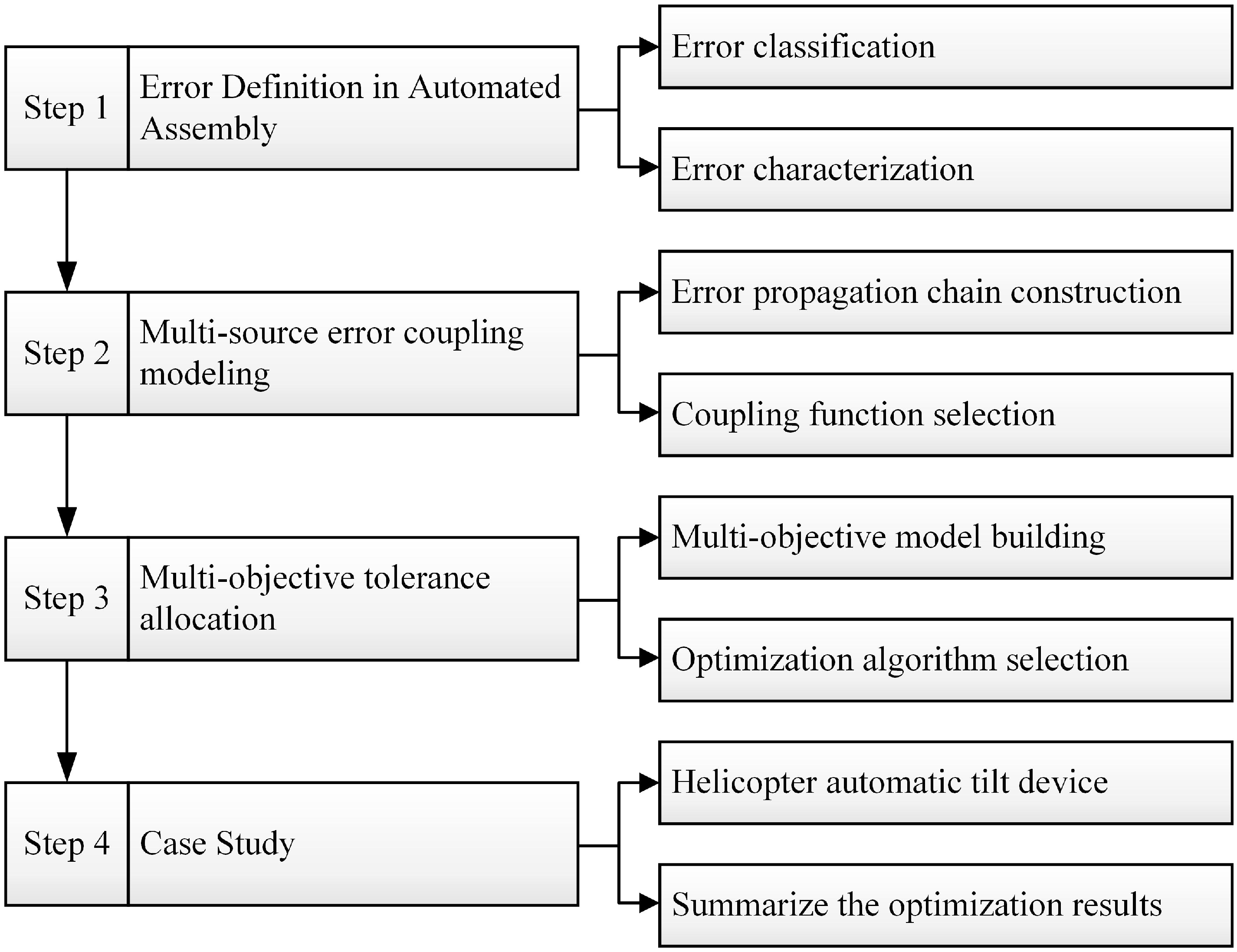
Figure 1. Overall implementation architecture of the proposed tolerance optimization method for automated assembly. The process includes four steps: (1) error definition and classification in automated assembly; (2) modeling of multi-source error coupling and propagation; (3) multi-objective tolerance allocation through simulation and optimization; and (4) application to a case study involving a helicopter automatic tilt device. Each step is further divided into key tasks as shown.
Machines 13 00736 g001
Figure 2. Comparison of traditional manual vs. automated assembly error chains. Manual assembly involves localized, discrete, and linear accumulation of tolerances with datum references, while automated assembly leads to globally continuous, nonlinear error propagation due to automation- and execution-induced uncertainties. The red text highlights automation-specific challenges.
Machines 13 00736 g002
Figure 3. Multi-source error classification in automated assembly.
Machines 13 00736 g003
Figure 4. Adjacency-aware multi-source error coupling network. Each part has three input error types: geometric deviation ( Δ M ), measurement error ( Δ A ), and process error ( Δ P ), which propagate through the coupling network to influence overall assembly deviation ( Δ _ f e a t u r e ). The equation block corresponds to Equation (14), where ϵ k represents an error source, and a k , b k , c k l are coefficients. The term k < l in the summation ensures cross-terms are counted only once, indicating interaction between error sources k and l.
Machines 13 00736 g004
Figure 5. Flowchart of the multi-objective tolerance optimization process integrating uncertainty simulation, sensitivity analysis, and evolutionary optimization.
Machines 13 00736 g005
Figure 6. Key assembly features in helicopter rings: (a) The simulant of helicopter rings. (b) Position accuracy between rings. (c) Coaxiality between rings.
Machines 13 00736 g006
Figure 7. Error analysis process between helicopter rings: (a) Define the fit between rings; (b) establish measurement of key quality metrics between rings, including position and coaxiality; and (c) define Δ M , Δ A , and Δ P errors.
Machines 13 00736 g007
Figure 8. Position and coaxiality results of 20,000 Monte Carlo analyses between rings, with the purple “Max” indicating the maximum observed deviation in the dataset. (a) Position deviation: Pass rate = 67.4%, CPK = 0.31; (b) Coaxiality deviation: Pass rate = 93.5%, CPK = 0.62.
Machines 13 00736 g008
Figure 9. Comparison of position (a) and coaxiality (b) deviation distributions under different tolerance optimization strategies. NSGA-II and SPEA2 are full multi-objective optimizations, while the other cases only optimize individual sources. NSGA-II shows the most concentrated distribution and highest CPK values, indicating the best overall improvement in assembly quality.
Machines 13 00736 g009
Table 1. Definitions and mathematical expressions of various error sources involved in the automated assembly process.
Error SourcesMathematical ExpressionsDistribution Type
Manufacturing geometric deviation δ d i = d i m e a s d i n o m N μ d , σ d 2
Surface topography errors R a = 1 L 0 1 z x d x L o g - N μ r , σ r 2
Repeat positioning error Δ p , Δ θ N 0 , σ p 2 , N 0 , σ p 2
Sensor/vision measure uncertainties y ¯ = y + b + ε N 0 , σ ε 2
Actuator dynamic response error δ F
Control latency and synchronization offsets τ , Δ t i j N 0 , σ ε 2 , N 0 , σ Δ t 2
Disclaimer/Publisher’s Note: The statements, opinions and data contained in all publications are solely those of the individual author(s) and contributor(s) and not of MDPI and/or the editor(s). MDPI and/or the editor(s) disclaim responsibility for any injury to people or property resulting from any ideas, methods, instructions or products referred to in the content.