Article

Modeling and Adaptive Neural Control of a Wheeled Climbing Robot for Obstacle-Crossing

1
Ocean College, Zhejiang University, Zhoushan 316000, China
2
Zhejiang University Robotics Institute, Yuyao 315400, China
3
Haichuang Humanoid Robot Industry Innovation Center, Hangzhou 311100, China
*
Author to whom correspondence should be addressed.
Machines 2025, 13(8), 674; https://doi.org/10.3390/machines13080674 (registering DOI)
Submission received: 25 June 2025 / Revised: 20 July 2025 / Accepted: 24 July 2025 / Published: 1 August 2025
(This article belongs to the Section Robotics, Mechatronics and Intelligent Machines)

Abstract

The dynamic model of a wheeled wall-climbing robot exhibits stage-specific changes when traversing different types of obstacles and during various stages of obstacle negotiation. Previous studies often employed remote control methods for obstacle-crossing control, which fail to dynamically adjust the torque distribution of magnetic wheels in response to real-time changes in the dynamic model. This limitation makes it challenging to precisely control the robot’s speed and attitude angles during the obstacle-crossing process. To address this issue, this paper first establishes a staged dynamic model for the wall-climbing robot under typical obstacle-crossing scenarios, including steps, 90° concave corners, 90° convex corners, and thin plates. Secondly, an adaptive controller based on a radial basis function neural network (RBFNN) is designed to effectively compensate for variations and uncertainties during the obstacle-crossing process. Finally, comparative simulations and physical experiments demonstrate the effectiveness of the proposed method. The experimental results show that this method can quickly respond to the dynamic changes in the model and accurately track the trajectory, thereby improving the control precision and stability during the obstacle-crossing process.

1. Introduction

In the long-term usage of steel-structure buildings, defects such as corrosion, cracks, and weld seam detachment may develop on their surfaces, necessitating regular inspections to ensure structural safety. The presence of obstacles on these surfaces, including steps, 90° concave corners, 90° convex corners, and thin plates, imposes stringent demands on the obstacle-crossing capabilities of inspection equipment. To meet the diverse requirements of application scenarios and tasks, researchers have developed a variety of wall-climbing robots with enhanced obstacle-crossing capabilities. These robots can be broadly categorized into three types based on their movement mechanisms: wheeled, legged, and tracked. Among these, wheeled robots are widely used in practical engineering applications due to their high mobility, simple structure and control, and low maintenance costs.
During obstacle-crossing, wall-climbing robots are influenced by several forces, including magnetic wheel adhesion, gravity, friction, and driving force. The magnitude and relative direction of these forces vary with the shape and size of the obstacle, the robot’s posture, and the load conditions, resulting in a dynamic and complex time-varying behavior in the robot’s dynamic model. Currently, the control of wheeled wall-climbing robots during obstacle-crossing primarily relies on manual remote operation, with a constant-speed control strategy typically employed to drive the magnetic wheels and perform the crossing action. While such strategies can meet basic obstacle-crossing requirements, they fail to account for the dynamic changes in forces during the process. This limitation prevents the dynamic adjustment and distribution of magnetic wheel torque, restricting further improvements in the efficiency and stability of obstacle-crossing. Therefore, optimizing obstacle-crossing performance requires a deeper understanding of the robot’s dynamic characteristics during the crossing process and the development of efficient control strategies to enable precise control of complex obstacle-crossing maneuvers.
In terms of dynamic modeling, existing research has primarily focused on static analysis of extreme conditions for different types of obstacles. For instance, studies [1,2,3,4,5,6,7] have developed detailed models for wheeled robots traversing typical obstacles such as steps, 90° concave corners, 90° convex corners, and thin plates. These models consider factors such as magnetic adhesion force, gravity, friction, and driving force to calculate the required magnetic adhesion force to prevent overturning and the driving torque necessary for successful obstacle-crossing. These findings provide valuable theoretical guidance for robot structural design. However, most of these studies are limited to specific conditions and do not fully consider the dynamic effects of obstacle shape, robot posture, and load variations during the crossing process. Consequently, their application to real-time obstacle-crossing control remains limited.
In the field of obstacle-crossing control for wheeled wall-climbing robots, existing studies predominantly focus on validating the obstacle-crossing performance of robots through remote control methods [7,8,9,10,11,12,13,14,15,16,17], while relatively few address the development of control strategies during the crossing process. For example, Baoyu Wang et al. [6] proposed a heavy-duty wall-climbing robot capable of overcoming inner right-angle obstacles. By establishing a kinematic model based on geometric constraints and employing different speed control strategies for the front and rear magnetic wheels during the crossing process, they effectively enhanced the robot’s stability. In related fields, some obstacle-crossing control methods have been implemented. For instance, Qingfang Zhang et al. [12] addressed the control requirements of a dual-propeller wall-climbing robot, DP-Climb, when crossing 90° concave corners. They proposed a PID-based tracking strategy designed using a dynamic obstacle-crossing model. The PID controller precisely tracked changes in speed and inclination during the crossing process and adjusted the propellers’ orientation in real time to optimize thrust and adhesion forces, achieving a smooth transition between inner right-angle wall surfaces. For wheeled robots crossing steps, various control algorithms have been proposed, including PID control [13], adaptive control [14], linear quadratic regulators [15], and state feedback control [16]. These approaches aim to track ideal changes in speed and posture during the step-crossing process. While these methods perform well under specific conditions, they face challenges in addressing complex and dynamic obstacle-crossing scenarios.
To address the challenges within modeling and control of a wheeled climbing robot, this paper presents the following key contributions: (1) Existing dynamic models for obstacle-crossing are often static or limited to specific conditions, failing to capture the full time-varying nature across the entire crossing process for diverse obstacles. We establish a comprehensive staged dynamic model for a four-wheeled magnetic wall-climbing robot using the Newton–Euler equations. This model explicitly covers the entire crossing process for four typical obstacle scenarios (steps, 90° concave corners, 90° convex corners, and thin plates), capturing the phase transitions and force variations. (2) Current control strategies lack the adaptability to compensate for the significant uncertainties and time-varying dynamics inherent in the obstacle-crossing process, leading to imprecise speed and attitude control. We develop a novel adaptive obstacle-crossing control strategy utilizing a radial basis function neural network (RBFNN). This controller is specifically designed to dynamically compensate for model variations and uncertainties in real time, enabling precise tracking of ideal speed and angular velocity trajectories throughout the complex crossing maneuvers.

2. Materials and Methods

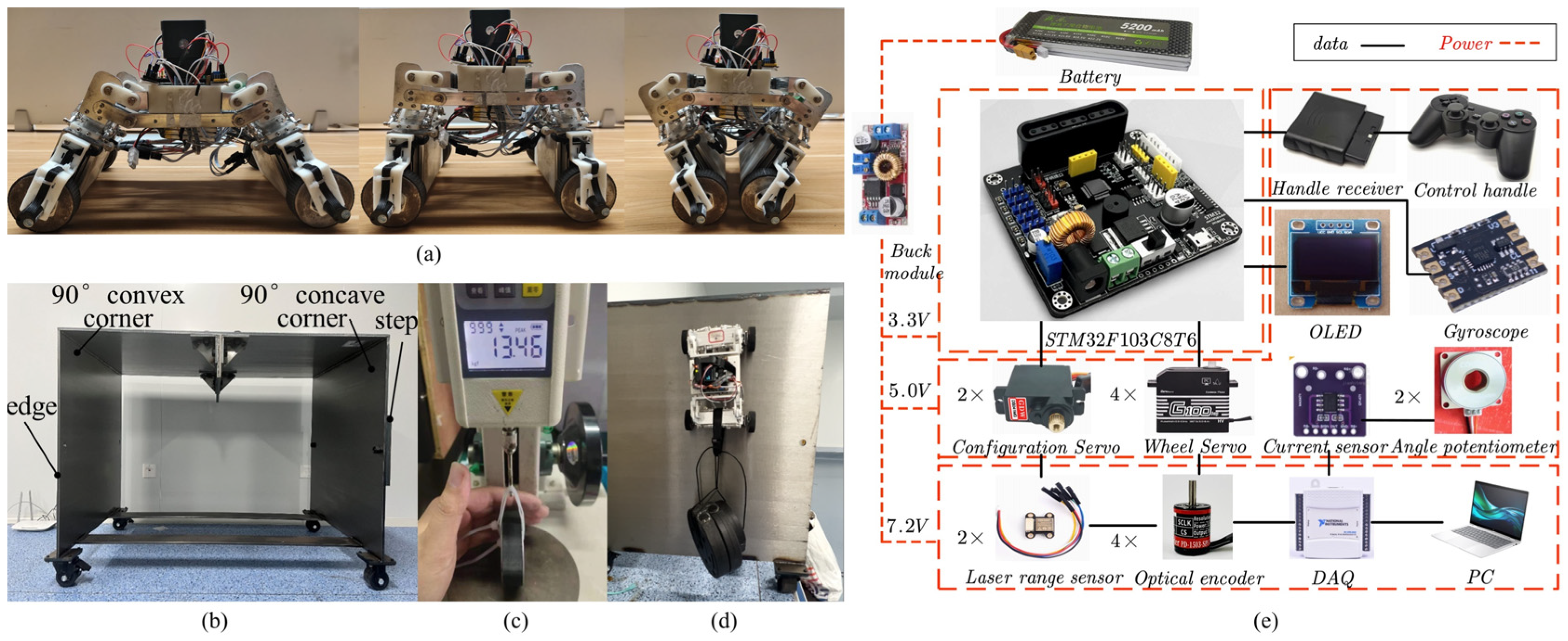
2.1. Mechanical Structure and the Obstacle-Crossing Principle

To address the requirements of crossing four typical types of obstacles, we designed a four-wheeled wall-climbing robot equipped with permanent magnetic wheels. As shown in Figure 1a, the robot features a symmetric structural design, where each magnetic wheel provides adhesion force and is independently driven by a servo motor. Based on a reconfigurable design principle, the robot can adapt its configuration to overcome various obstacle types, as illustrated in Figure 1b–f. Before crossing an obstacle, the robot uses its configuration adjustment mechanism to flexibly modify the distance between wheel centers. Depending on the type of obstacle, the robot selects an appropriate configuration to ensure geometric passability. As depicted in Figure 1b, the robot has three configurations, labeled A, B, and C from left to right. Configuration A is characterized by the maximum distance between the front and rear magnetic wheel centers. This configuration is suitable for crossing steps and 90° concave corners. In this setup, the increased wheel center distance allows for a larger frictional arm (indicated by the blue arrow), providing greater rotational torque during the crossing process Configuration B is designed to meet the geometric constraints of crossing 90° convex corners. In this configuration, the robot ensures that the chassis does not collide with the convex corner of the 90° convex corner during the crossing process. Configuration C features the minimum distance between the front and rear magnetic wheels, which is smaller than the thickness of the thin plate. This configuration is tailored for crossing thin plates, ensuring that the chassis does not collide with the plate’s edge during the crossing process. The state transitions of the robot while crossing different obstacles are shown in Figure 1c–f:

2.2. Kinematic Modeling for Obstacle-Crossing

The kinematic constraints of the robot under various obstacle-crossing scenarios can be described using a unified kinematic model. As illustrated in Figure 2, the world coordinate system is defined as {XYZO}, and the robot’s state is denoted as [x, z, β, α1, α2], where x and z represent the coordinates of the robot’s center of gravity P in the world coordinate system, O1, O2 are the positions of the front and rear magnetic wheel centers, respectively, and β is the angle between the robot body and the horizontal surface. The front magnetic wheel has a linear velocity v1 and rotational angle α1, while the rear magnetic wheel has a linear velocity v2 and rotational angle α2.
Assuming no lateral slip occurs during wheel movement and the wheels maintain pure rolling on the surface, the following nonholonomic constraint equations can be established:
x ˙ 1 cos θ 1 + z ˙ 1 sin θ 1 = α ˙ 1 r x ˙ 2 cos θ 2 + z ˙ 2 sin θ 2 = α ˙ 2 r ,
where [x1, z1] and [x2, z2] are the coordinates of the front and rear wheel centers, r is the magnetic wheel radius, and θ1 and θ2 are the angles between the velocity directions of the front and rear wheels and the X-axis, respectively.
From the geometric constraint that the distance between O1 and O2 equals L, we obtain:
x ˙ 1 = x ˙ L 2 β ˙ sin β z ˙ 1 = z ˙ + L 2 β ˙ cos β x ˙ 2 = x ˙ + L 2 β ˙ sin β z ˙ 2 = z ˙ L 2 β ˙ cos β ,
and the kinematic constraint equation F(q) q ˙ = 0 can be derived, where F(q) is:
cos θ 1 sin θ 1 L 2 sin ( β θ 1 ) r 0 cos θ 2 sin θ 2 L 2 sin ( β θ 2 ) 0 r ,

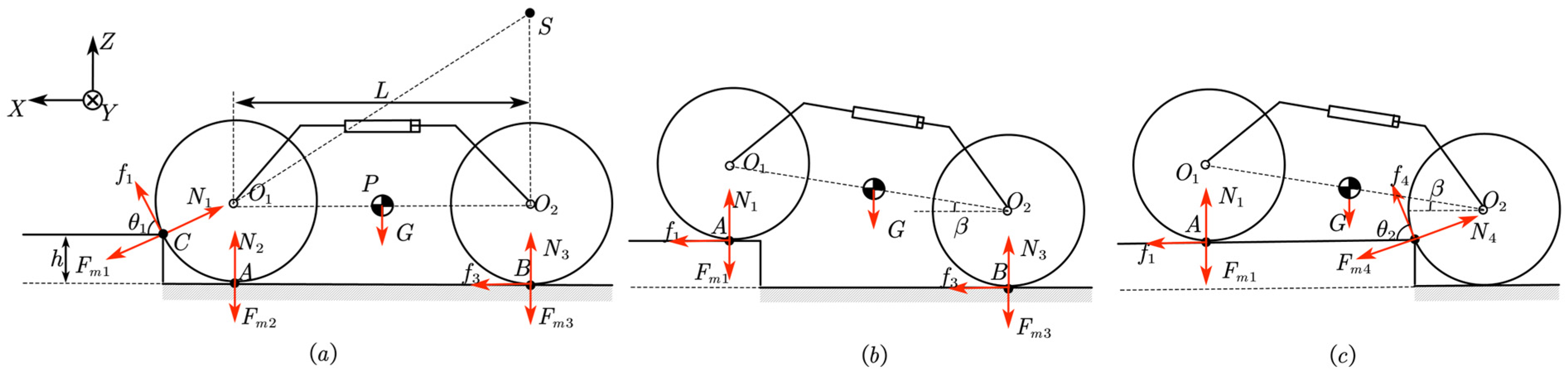
2.3. Phase-Based Obstacle-Crossing Dynamics Modeling

Due to significant differences in the force states of the climbing robot during different obstacle types and crossing stages, separate phase-based dynamic models have been developed for each crossing condition to more accurately describe the robot’s dynamic characteristics during the obstacle-crossing process.

2.3.1. Step

The phase-based dynamic model for the robot crossing a step is first established. As shown in Figure 3a–c, the process of crossing the step is divided into three stages.
Stage 1: The front magnetic wheel of the robot contacts the step’s convex edge and rotates around the edge until the front wheel completes the step crossing. During this phase, the robot performs rotational motion around point S. Stage 2: Both the front and rear magnetic wheels move horizontally along the axis direction until the rear magnetic wheel contacts the step’s convex edge. Stage 3: The rear magnetic wheel rotates around the step’s convex edge until it completes the step crossing.
Define the origin as shown in Figure 3a, and establish the mechanical equilibrium equations along the X- and Z-axes. Along point S, establish the moment equilibrium equation. The first-stage dynamic equation can be obtained as:
m x ¨ = sgn ( f 1 ) ( 2 f 1 cos θ 1 + 2 f 3 ) m z ¨ = sgn ( f 1 ) ( 2 f 1 sin θ 1 2 F m 2 G 2 ) J β ¨ = sgn ( f 1 ) [ 2 f 1 ( L sin θ 1 + r ) 2 F m 2 L G L 2 + 2 f 3 ( L tan θ 1 + r ) ] T f = m w α ¨ 1 r 2 , T r = m w α ¨ 2 r 2 T f = f 1 r , T r = f 3 r ,
where fi is the friction force between the magnetic wheel and the wall surface, Ni is the supporting force acting on the magnetic wheel, and Fmi is the magnetic attraction force acting on the magnetic wheel. G represents the robot’s weight, m is the total mass, mw is the magnetic wheel mass, r is the radius of the magnetic wheel, and u is the wall friction coefficient. J is the moment of inertia, Tf is the driving torque of the front magnetic wheel, and Tr is the driving torque of the rear magnetic wheel. When the front magnetic wheel detaches from the horizontal wall, N2 = f2 = 0. Based on the geometric constraints, the robot’s climbing process will satisfy the following relationship between θ1 and θ2:
θ 1 = arccos r h + z 1 r , θ 2 = 0 ,
and in Equation (4), sgn (f1) is the judgment function for the detachment of the front magnetic wheel from the horizontal wall. As shown in Figure 3a, the magnetic wheel needs to meet the climbing condition in order to successfully climb over the step. Specifically, the component of the friction force f1 along the Z-axis must be greater than the sum of the magnetic attraction force Fm2 and the weight of the magnetic wheel. The judgment function designed based on the climbing condition is:
sgn ( f 1 ) = 1 , i f 2 f 1 sin θ 1 2 F m 2 G 2 > 0 0 , e l s e ,
and the first-stage obstacle-climbing dynamic model can be derived as:
M 11 ( q ) q ¨ + E 11 ( q ) F m + N 11 ( q ) G = B 11 ( q ) τ ,
where Fm = [Fm1 Fm2 Fm3 Fm4], τ = [Tf Tr].
By differentiating the kinematic Equation (4) with respect to time, we obtain:
q ¨ = S ˙ ( q ) η + S ( q ) η ˙ ,
substituting Equation (8) into the dynamic Equation (7), the dynamic equation can be rewritten as:
η ˙ = f ( η , F m ) + B ¯ τ ,
where f(η,Fm) = − M - ( N - η + EFm + G) M -   =   (MS)−1, N -   =   M S ˙ and B -   =   (MS)−1 B. Similarly, the dynamic equations for the second and third stages can be derived.

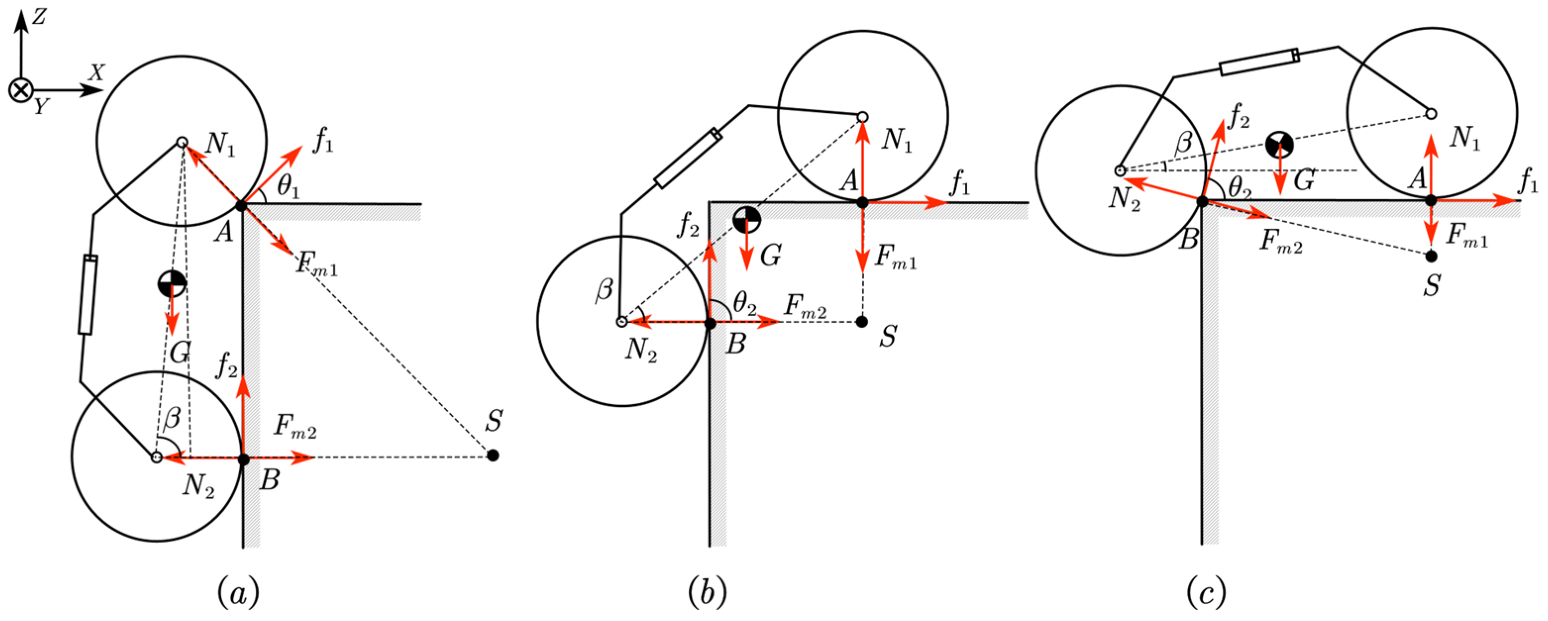
2.3.2. 90° Concave Corner

As shown in Figure 4, the robot’s process of climbing over an internal right angle is divided into two stages.
The robot’s initial state in the first stage is shown in Figure 4a. At this point, the front magnetic wheel is simultaneously attached to both the horizontal and vertical walls. The front magnetic wheel uses the friction force with the vertical wall to detach from the magnetic attraction force of the horizontal wall and moves along the vertical wall. Meanwhile, the rear magnetic wheel moves forward along the horizontal wall. During this process, the body tilt angle of the robot gradually increases until the rear magnetic wheel attaches to the vertical wall. In the second stage (Figure 4c), the rear magnetic wheel detaches from the horizontal wall, and the robot moves along the vertical wall.
Along the X- and Z-axes, establish the mechanical equilibrium equations. Then, around point S, establish the moment equilibrium equation for the robot. The first-stage dynamic equation can be obtained as follows:
m x ¨ = sgn ( f 1 ) 2 f 4 cos θ 2 m z ¨ = sgn ( f 1 ) ( 2 f 1 sin θ 1 + 2 N 2 2 F m 2 G 2 ) J y β ¨ = sgn ( f 1 ) 2 f 1 ( L cos β + r ) + 2 f 4 ( L sin β + r ) G L cos β 2 2 F m 2 L cos β T f = m w α ¨ 1 r 2 , T r = m w α ¨ 2 r 2 T f = f 1 r , T r = f 4 r ,
and in the above equation, the angle between the velocity direction of the front magnetic wheel and the xxx-axis is denoted as θ1 = π/2, and the angle between the velocity direction of the rear magnetic wheel and the xxx-axis is denoted as θ2 = 0. When the front magnetic wheel detaches from the horizontal wall, N2 = f2 = 0. Sgn(f1) is the judgment function for the detachment of the front magnetic wheel from the horizontal wall. For the front magnetic wheel to detach from the horizontal wall, the friction force f1 must be greater than the sum of the magnetic attraction force Fm2 on the horizontal wall and the robot’s weight. Based on this climbing condition, the judgment function is designed as:
sgn ( f 1 ) = 1 , i f ( 2 f 1 2 F m 2 G 2 ) > 0 0 , e l s e ,
the process of deriving the dynamic equations under the step-climbing condition is the same. By simplifying the equations above, we can obtain a dynamic equation of the same format as Equation (9). Similarly, the dynamic equations for the second and third stages can be derived.

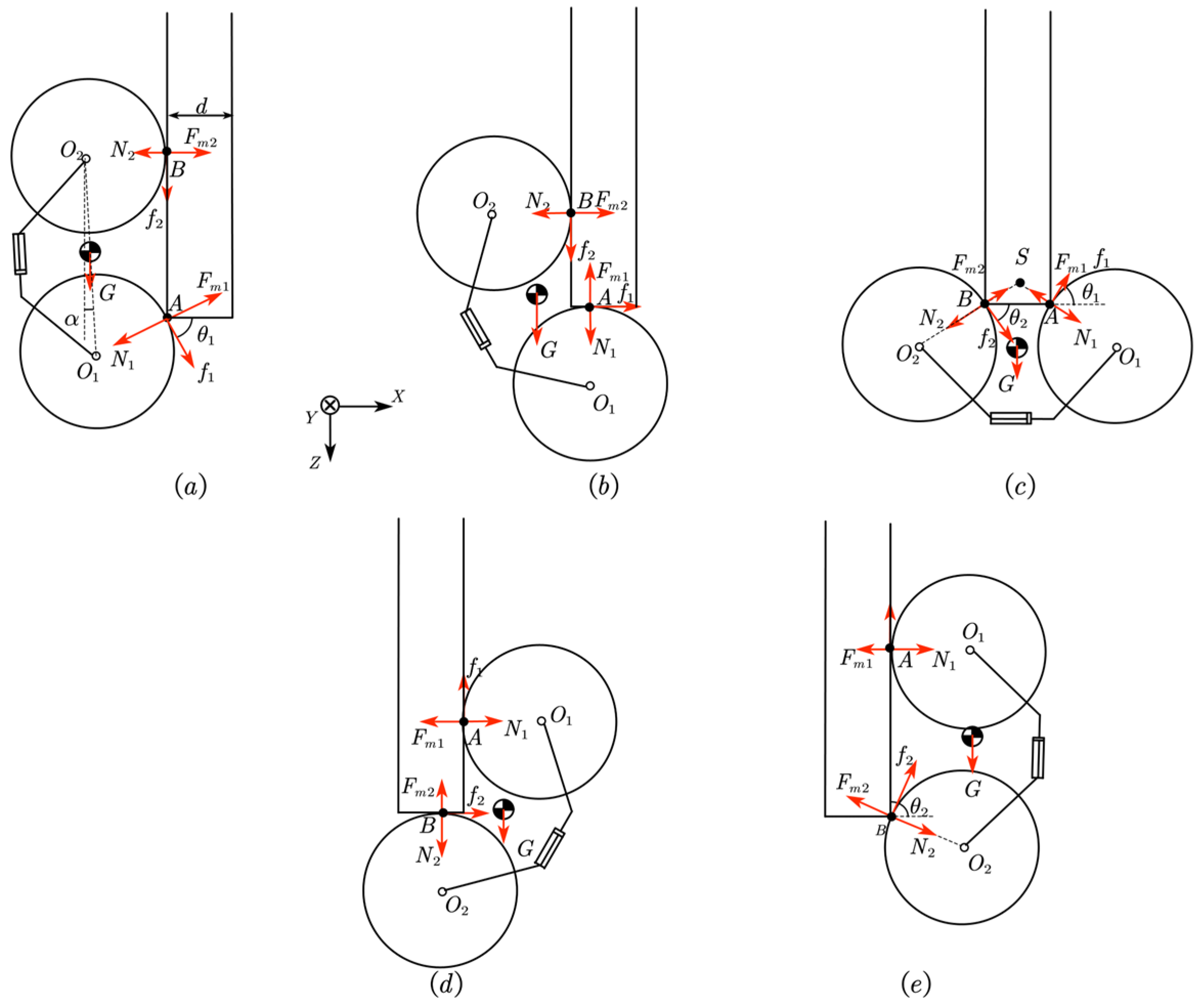
2.3.3. 90° Convex Corner

As shown in Figure 5, the robot’s process of climbing over an external right angle is divided into three stages. In the first stage (Figure 5a), the front magnetic wheel is attached to the convex corner of the external right angle. It rotates around the convex corner until the front magnetic wheel successfully climbs over the 90° convex corner. In the second stage (Figure 5b), the front magnetic wheel moves along the horizontal wall, while the rear magnetic wheel moves upward along the vertical wall. During this process, the body tilt angle of the robot gradually decreases until the rear magnetic wheel contacts the convex corner of the 90° convex corner. In the third stage (Figure 5c), the rear magnetic wheel rotates around the convex corner until it successfully climbs over the convex corner. At this point, both the front and rear magnetic wheels are attached to the horizontal wall.
Along the X- and Z-axes, establish the mechanical equilibrium equations. Then, around point S, establish the moment equilibrium equation for the robot. The dynamic equation for the first stage can be obtained as Equation (12). In this equation, the angle between the velocity direction of the front magnetic wheel and the X-axis is denoted as θ1 = arccos(z1/r), and the angle between the velocity direction of the rear magnetic wheel and the X-axis is denoted as θ2 = π/2. Similarly, the phased dynamic model for the robot climbing over an internal right angle can be derived.
m x ¨ = 2 f 1 cos θ 1 + 2 f 2 cos θ 2 m z ¨ = 2 f 1 sin θ 1 + 2 f 2 sin θ 2 G J y β ¨ = 2 f 1 ( L sin β R cos θ 1 ) cos θ 1 + 2 f 2 ( L sin β R cos θ 1 ) tan θ 1 G L cos β 2 + L sin β tan θ 1 T f = m w α ¨ 1 r 2 , T r = m w α ¨ 2 r 2 T f = f 1 r , T r = f 2 r .

2.3.4. Thin Plate

The robot’s process of climbing over a thin plate is divided into five stages, as shown in Figure 6. In the first stage (Figure 6a), the front magnetic wheel rotates around the left convex corner of the thin plate, while the rear magnetic wheel moves downward along the vertical wall, until the front magnetic wheel successfully climbs over the convex corner. In the second stage (Figure 6b), the front magnetic wheel moves along the horizontal wall of the thin plate, while the rear magnetic wheel continues to move downward along the vertical wall, until the front magnetic wheel contacts the right convex corner of the thin plate. In the third stage (Figure 6c), the front and rear magnetic wheels are each attached to the convex corners on both sides of the thin plate, rotating around their respective corners. In the fourth stage (Figure 6d), the front magnetic wheel moves upward along the vertical wall, while the rear magnetic wheel moves along the horizontal wall of the thin plate. In the fifth stage (Figure 6e), the front magnetic wheel moves upward along the vertical wall, while the rear magnetic wheel rotates around the right convex corner of the thin plate until the rear magnetic wheel successfully climbs over the convex corner.
Except for the third stage, the force conditions for the robot in the other stages are the same as those described in Section 2.3.3 for the 90° convex corner condition. Therefore, the same dynamic model can be used to describe these stages. However, for the climbing robot’s process of overcoming a thin plate, the dynamic model for the third stage is unique and requires a separate dynamic equation:
m x ¨ = 2 f 1 cos θ 1 + 2 f 2 cos θ 2 m z ¨ = 2 f 1 sin θ 1 + 2 f 2 cos θ 2 G J y β ¨ = 2 f 1 d ( tan θ 1 + tan θ 2 ) cos θ 1 + 2 f 2 d ( tan θ 1 + tan θ 2 ) cos θ 2 G L cos β 2 T f = m w α ¨ 1 r 2 , T r = m w α ¨ 2 r 2 T f = f 1 r , T r = f 2 r ,
in which the angle between the velocity direction of the front magnetic wheel and the X-axis is denoted as θ1 = arccos(z1/r), and the angle between the velocity direction of the rear magnetic wheel and the X-axis is denoted as θ2 = arccos(z2/r).

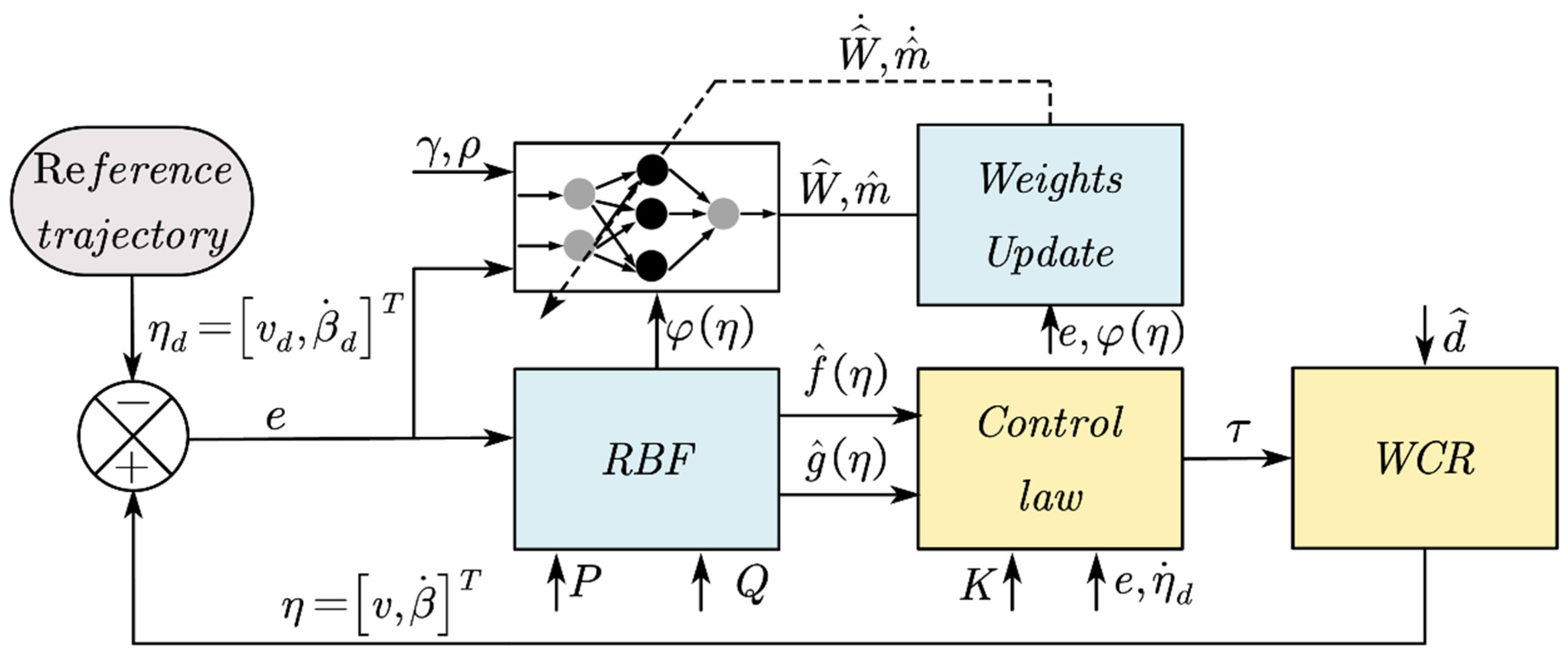
2.4. Obstacle Climbing Motion Control Based on Radial Basis Function Neural Network Compensation

During the obstacle-climbing process, the variations in the magnetic wheel’s adhesion force and the uncertainties caused by external disturbances make it challenging to establish an accurate dynamic model. Therefore, in this section, the radial basis function neural network (RBFNN) is used to compensate for the dynamic model. Since RBFNNs could approximate nonlinear functions, they are widely used to approximate unknown nonlinear functions in dynamic models. The dynamic models for the robot climbing over obstacles under different conditions were established, and the expressions are given by:
η ˙ = f ( η , F m ) + g ( η ) τ ,
the ideal trajectory of the robot ηd is known. The tracking error of the system is defined as:
e = η d η ,
by differentiating both sides of this equation with respect to time, we obtain:
e ˙ = η ˙ d η ˙ = η ˙ d f ( η ) g ( η ) τ ,
following by defining the Lyapunov function L = eTe/2, and differentiate it to obtain:
L ˙ = e e ˙ = e ( η ˙ d f ( η ) g ( η ) τ ) ,
the above equation needs to satisfy L ˙   < 0 to ensure ( η ˙ df(η) − g(η)τ) = −Ke. The system control law τ is designed as:
τ = g ( η ) 1 ( K e f ( η ) + η ˙ d ) ,
where K is a semi-positive definite diagonal matrix. The functions f(η) and g(η) are bounded smooth functions that satisfy ηi∈Ω∈Rn, |f(η)| ≤ fmax, |g(η)| ≤ gmax.
Figure 7 shows the structure of the RBF neural network, which consists of an input layer, a hidden layer, and an output layer. Due to uncertainties in the dynamic model and external disturbances, both f(η) and g(η) are unknown. In practical applications, control inputs τ cannot be directly applied, so the RBF neural network is used to approximate the unknown terms in the dynamic model:
f ( η ) = W T φ ( η ) + ε 1 ( η ) ,
g ( η ) = N T ψ ( η ) + ε 2 ( η ) ,
where W and N represent the target weights of the neural network output layer, l is the number of neurons, εi is the approximation error, and φ (η) is the system activation function. φ(η) = [φ1(η), φ2(η),…, φl(η)]T. The activation function used is the Gaussian radial basis function, given by:
φ i ( η ) = exp η u i 2 2 σ i 2 , i = 1 , 2 , , n ,
where ui and σi represent the center and radial width of the i-th neuron, respectively.
To ensure that the RBF neural network can approximate any nonlinear function, the following assumption is made:
Assumption 1.
There exist optimal weight parameters W* such that the approximation error of the nonlinear function w satisfies:
w = f ^ ( η | W * ) f ( η ) < ξ ,
The estimated output values of the RBFNN are defined as  f ^ =   W ^ T φ η and g ^ =   N ^ T ψ η , which approximate the functions, respectively. The function approximation errors are denoted as f ~ η = f η f ^ ( η ) and g ~ η = g η g ^ ( η ) , where f ~ and g ~ represent the estimation errors.
Thus, Equation (18) can be rewritten as:
τ = g ^ ( η ) 1 ( K e f ^ ( η ) + η ˙ d ) ,
and the optimal weight values are defined as:
W * = arg min w Ω [ sup | f ^ ( η ) f ( η ) | ] ,
where sup represents the least upper bound, which is the maximum output value of the function for all possible input values.
The Lyapunov function is defined as:
L 2 = 1 2 e T P e + 1 2 γ ( W ^ W * ) T ( W ^ W * ) + 1 2 ρ ( N ^ N * ) T ( N ^ N * ) ,
where γ is a symmetric positive definite matrix, W ^ W* and N ^ N* are the parameter estimation errors, and they satisfy the Lyapunov equation:
K T P + P K = Q ,
where Q ≥ 0 and ρ > 0. Define V1 = eTPe/2, V 2   =   1 2 γ W   ^   W * T W   ^   W * , V 3   =   1 2 ϱ N ^     N * T N   ^   N * , Ψ   = W ^     W * T φ η   +   w   +   [ g η     g ^ ( η ) ] τ . Equation (18) can be rewritten as:
e ˙ = K e + Ψ ,
combining above, we obtain:
L ˙ 2 = V ˙ 1 + V ˙ 2 + V ˙ 3 = 1 2 e T Q e + e T P w + 1 γ ( W * W ^ ) T [ W ^ ˙ + γ e T P φ ( η ) ] + m ˜ ( e T P τ 1 ρ m ^ ˙ ) ,
defining the weight update rate as:
W ^ ˙ = γ e T P φ ( η ) ,
to ensure that m ~ e T P τ ρ m ^ ˙ 0 , reference [18] uses an adaptive update strategy to update:
m ^ ˙ = 1 ρ e T P τ ,   if   e T P τ > 0 1 ρ e T P τ ,   if   e T P τ 0   and   m ^ > m ¯ 1 ρ ,   if   e T P τ > 0   and   m ^ m ¯ ,
when m   ^ ˙   >   0 , m ^   >   m - .
Substituting the weight update rates (29) and (30) into Equation (28), we obtain:
L ˙ 2 = 1 2 e T Q e + e T P w
when the estimation error w using the RBF network approximation is sufficiently small, the system we obtain is Uniformly Ultimately Bounded (UUB).

3. Results

3.1. The Simulation Experiment

To verify the effectiveness of the proposed control method, the controller’s tracking performance under four different obstacle-crossing conditions was tested in the Matlab R2023b simulation environment. The time period was set to 0.01 s. The controller framework is shown in Figure 8, and the ideal trajectories of the robot under different obstacle-crossing conditions are calculated using Equation (26). In this section, the proposed control method is compared with adaptive control [19] and neural network control [20], with the control parameters for comparison being well selected and adjusted. The relevant parameters of the obstacle-crossing dynamic model are shown in Table 1:

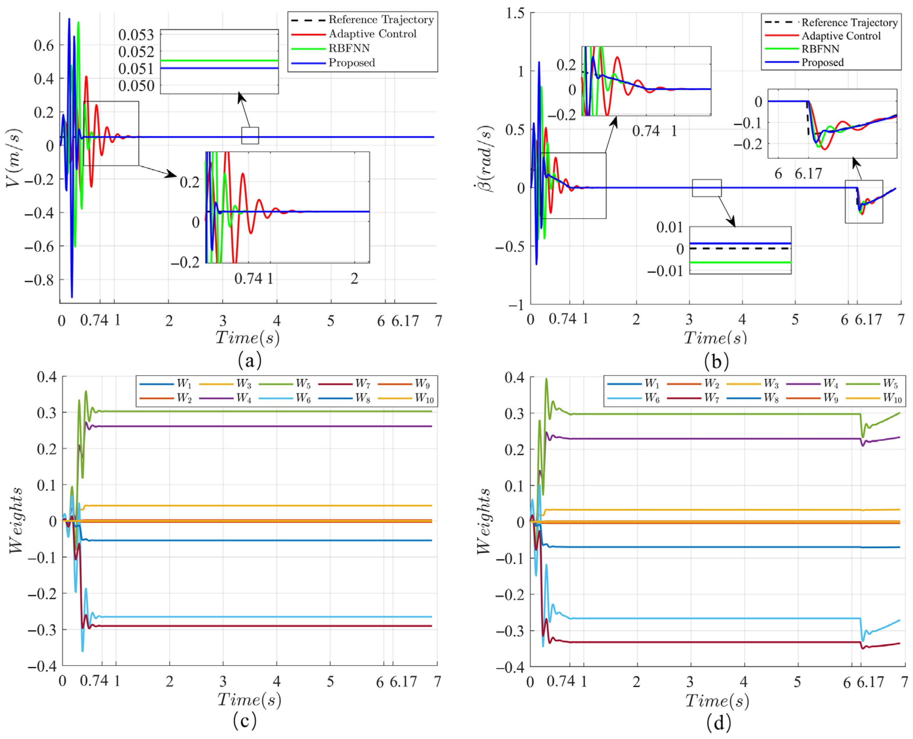
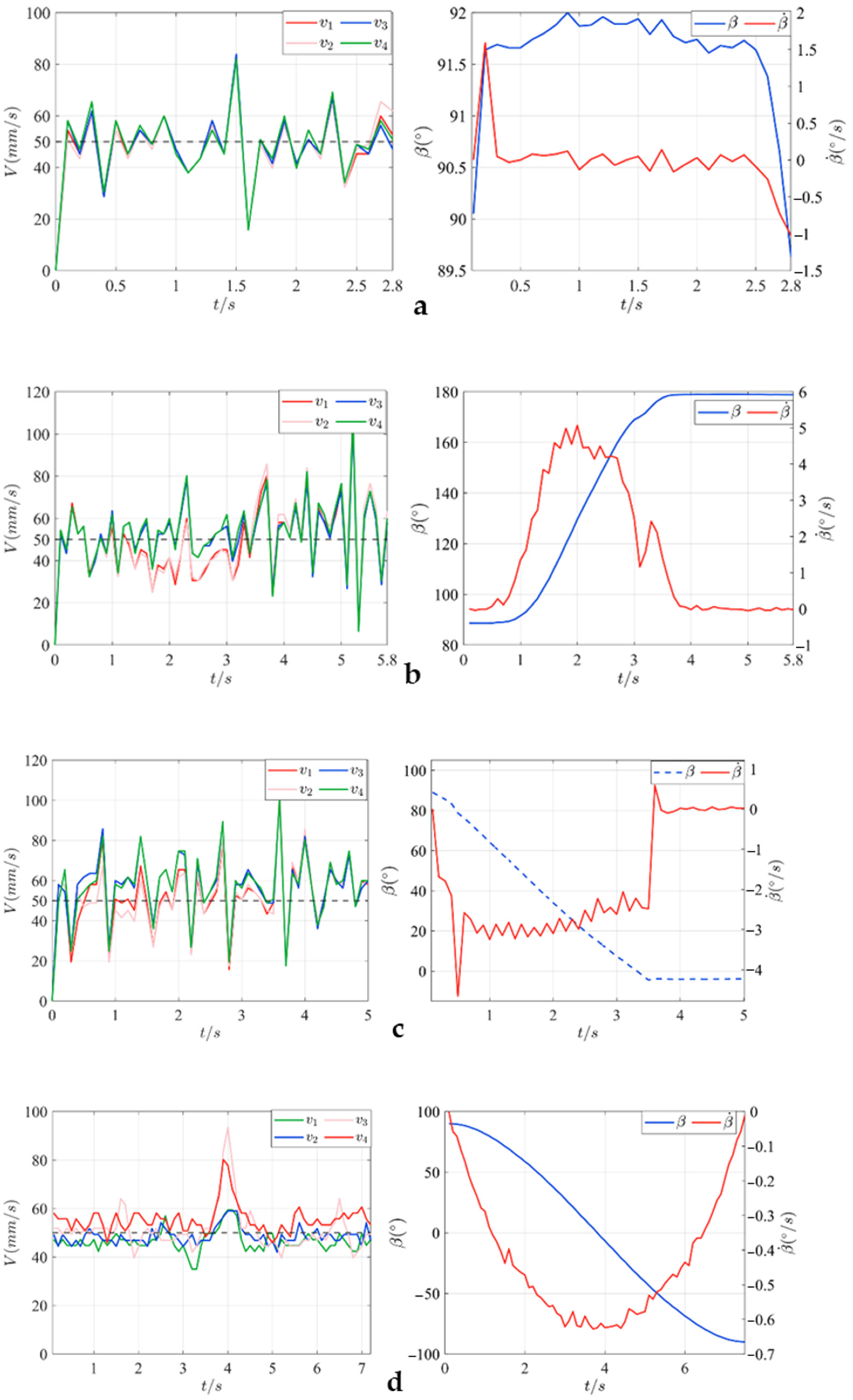
3.1.1. The Step Climbing Control Experiment

The robot’s front and rear magnetic wheel centers are set with a center distance of L = 250 mm, and the ideal speed of the front magnetic wheel is vd = 0.05 m/s. The initial conditions of the robot are v(0) = 0, β(0) = 0, θ1(0) = arccos(rh/r), θ2(0) = 0, τ(0) = [0, 0]T. The controller parameters are K = diag [100, 100], Q = diag [10, 10], and the weight learning rate is γ = [1.33, 1.2]T, ρ = [2, 2.1]T. The number of neurons in the RBFNN is set to l = 10. The initial weights are set to W0 = [01 × 10]T, with the Gaussian radial basis function centers at u1 = [−0.05; −0.025; 0; 0.025; 0.05] and the radial basis width u2 = [−8; −0.4; 0; 4; 8].
As shown in Figure 9a,b, the results of velocity and angular velocity tracking are compared between the proposed control strategy, adaptive control, and RBFNN control. The black dashed line represents the reference trajectory, the red curve is the result of adaptive control, the green curve is the output of the RBFNN control, and the blue curve is the output of the proposed control method. The robot’s step climbing process is divided into three stages, corresponding to time intervals t∈[0, 0.74], t∈[0.74, 6.17], and t∈[6.17, 6.91]. At the transition moments (when t = 0.74 and t = 6.17 change), the proposed method demonstrates significant performance advantages. Compared to adaptive control and RBFNN control, the proposed control strategy shows a notable reduction in oscillation amplitude, faster convergence speed, and more accurate tracking of the reference trajectory, exhibiting superior tracking precision and response speed.
Figure 9c,d correspond to the dynamic changes in the neural network weights during velocity tracking and posture angular velocity tracking. At time t=0, the wall-climbing robot begins the step climbing process, and the neural network weights start to update in real time. At time t = 0.74, the weights are adjusted to Wv = [0; 0.001; 0.021; 0.149; 0.192; −0.151; −0.156; −0.026; −0.001; 0] and Wβ = [0.001; 0.005; 0.090; 0.510; 0.596; −0.523; −0.731; −0.187; −0.014; −0.001], achieving precise tracking of the robot’s speed and pitch angular velocity. At time t = 6.17, the obstacle-crossing dynamic model transitions from phase two to phase three, and Wv remain constant. During the subsequent trajectory changes, the weight values continue to adjust dynamically, ensuring that the tracking error converges quickly.

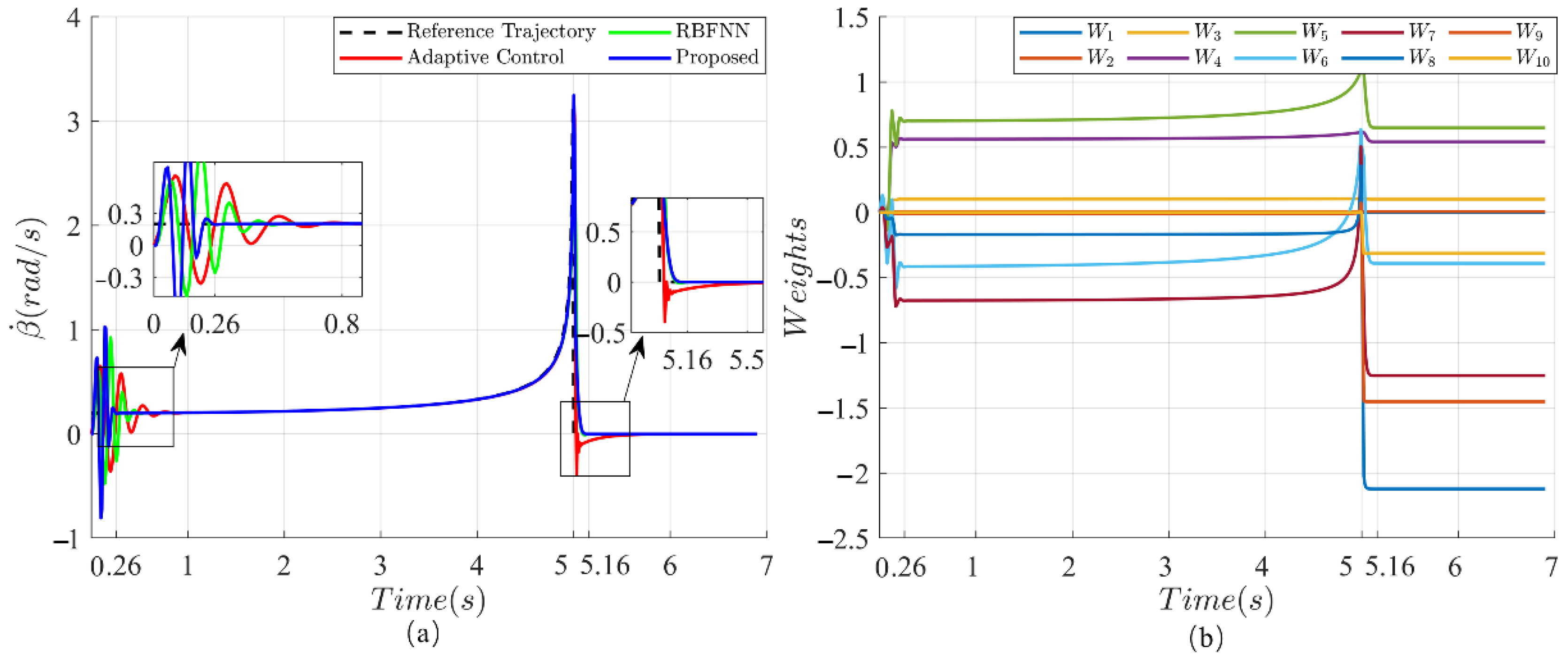
3.1.2. The 90° Concave Corner Climbing Control Experiment

The robot’s front and rear magnetic wheel center distance is set to L = 200 mm. The robot’s initial state is v(0) = 0, β(0) = 0, θ1(0) = π/2, θ2(0) = 0, τ(0) = [0, 0]T. The controller parameters are K = [100, 0; 0, 100], Q = [10, 0; 0, 10], and the weight learning rate is γ = [1.33, 1.2]T, ρ = [2, 2.1]T. The centers of the Gaussian radial basis functions are u1 = [−0.05; −0.025; 0; 0.025; 0.05], and the radial basis width is σ1 = 0.05, σ2 = 8.
As shown in Figure 10a, the wall-climbing robot’s step-over process at an internal right angle is divided into two stages corresponding to time intervals t∈[0, 5] and t∈[5, 7]. When t∈[5, 7], the robot begins climbing the internal right angle, and after 0.26 s, the proposed method’s weights achieve rapid convergence. The weights are adjusted to Wβ = [0.703; 0.561; 0.102; 0.005; 0.001; 0.001; −0.012; −0.170; −0.412; −0.676], and the error converges. In the initial stage (approximately 0.26 s), all control methods undergo rapid dynamic adjustments to follow the reference trajectory. The proposed method has a faster response speed, allowing it to approach the target trajectory earlier, while its oscillation amplitude is significantly lower than RBFNN and adaptive control, demonstrating superior dynamic stability.
At t = 5 s, the robot transitions from phase one to phase two, and the dynamic model changes quickly. The proposed method continues to adjust the control signals rapidly and stably. After 0.16 s, the weights are adjusted to Wβ = [0.650; 0.541; 0.100; −0.314; 0.005; 0.001; −0.392; −1.252; −1.453; −2.122], and the error quickly converges. However, the adaptive control (red curve) shows a significant deviation and oscillation during this stage.

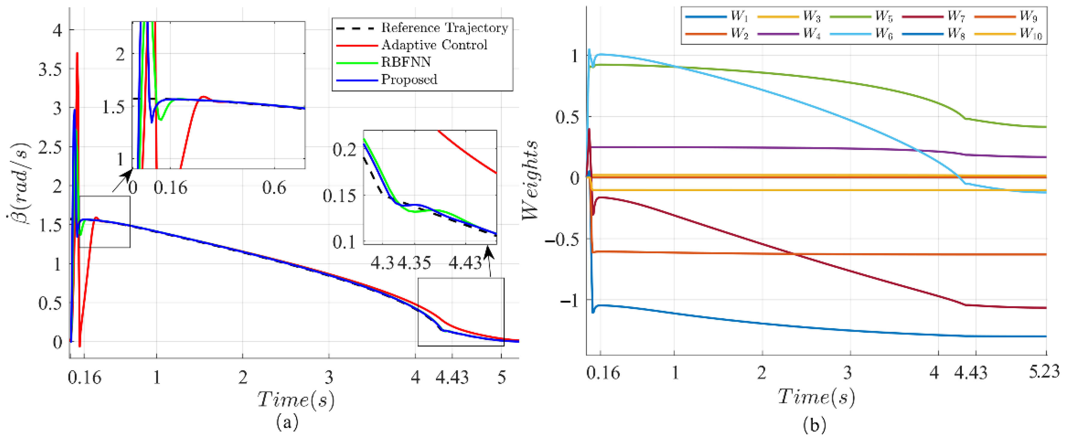
3.1.3. The 90° Convex Corner Climbing Control Experiment

The robot’s front and rear magnetic wheel center distance is set to L = 250 mm. The robot’s initial state is v(0) = 0, β(0) = 0, θ1(0) = π/2, θ2(0) = 0, τ(0) = [0, 0]T. The controller parameters are K = [100, 0; 0, 100], Q = [10, 0; 0, 10], and the weight learning rate is γ = [1.33, 1.2]T, ρ = [2, 2.1]T. The centers of the Gaussian radial basis functions are u1 = [−0.05; −0.025; 0; 0.025; 0.05] and u2 = [−8; −0.4; 0; 4; 8], and the radial basis width is σ1 = 0.05, σ2 = 8.
As shown in Figure 11a, the wall-climbing robot’s step-over process at an external right angle is divided into three stages corresponding to time intervals t∈[0, 0.94], t∈[0.94, 4.29] and t∈[4.29, 5.23]. When t = 0, the robot begins climbing the external right angle, and after 0.16 s, the weights converge rapidly, adjusting to Wβ = [1.007; 0.923; 0.249; 0.020; 0.001; 0.001; −0.102; −0.162; −0.605; −1.046], and then continue to change in response to the reference trajectory. In the initial response stage of the trajectory, the proposed method (blue curve) can quickly follow the reference trajectory (black dashed line), with the smallest overshoot and least oscillation. In contrast, although adaptive control (red curve) also follows the reference trajectory, it exhibits noticeable overshoot and significant oscillation.
At t = 4.29 s, the robot transitions from phase two to phase three. After 0.14 s, the weights are adjusted to Wβ = [0.469; 0.183; 0.017; 0.001; 0.001; −0.064; −0.103; −0.630; −1.047; −1.297], and the error rapidly converges. In the initial stage (approximately 0.26 s), all control methods undergo rapid dynamic adjustments to follow the reference trajectory. The proposed method has a faster response speed, allowing it to approach the target trajectory earlier, with significantly less oscillation than RBFNN and adaptive control, showing superior dynamic stability. The adaptive control method experiences more substantial deviation in this phase. RBFNN control has a slightly slower response, but its tracking accuracy is better than adaptive control.

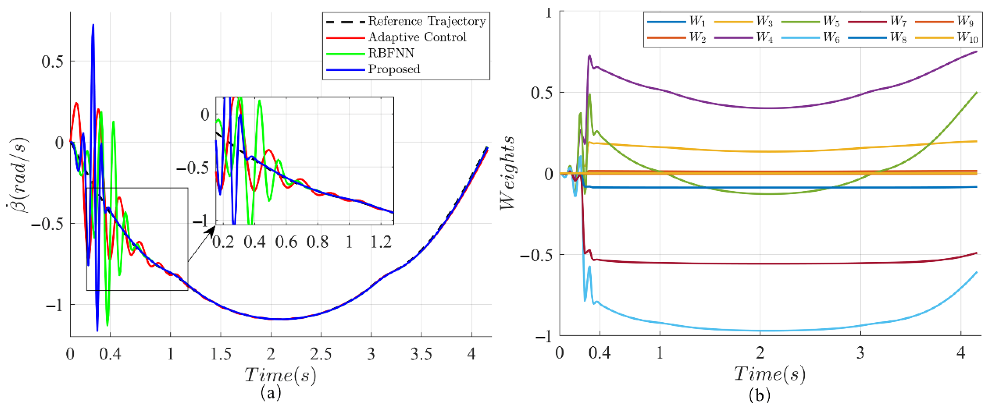
3.1.4. The Thin Plate Climbing Control Experiment

The front and rear magnetic wheel center distance of the robot is set to L = 70 mm. The robot’s initial state is v(0) = 0, β(0) = 0, θ1(0) = π/2, θ2(0) = 0, τ(0) = [0, 0]T. The controller parameters are K = [100, 0; 0, 100], Q = [10, 0; 0, 10], and the weight learning rate is γ = [1.33, 1.2]T, ρ = [2, 2.1]T. The centers of the Gaussian radial basis functions are u1 = [−0.05; −0.025; 0; 0.025; 0.05] and u2 = [−8; −0.4; 0; 4; 8], and the radial basis width is σ1 = 0.05, σ2 = 8.
As shown in Figure 12a, after a period of time, the wall-climbing robot begins to climb the thin plate. After 0.4 s, the proposed method achieves weight convergence. In the initial stage, it quickly approaches the reference trajectory, with the minimum overshoot and the lowest oscillation amplitude. In comparison, adaptive control, while able to follow the reference trajectory relatively quickly, exhibits significant overshoot and large oscillations. The RBFNN method has a slower response speed, but its tracking accuracy is better than that of adaptive control. Subsequently, as shown in Figure 12b, the neural network weights dynamically change as the tracking trajectory evolves. The trajectory tracking error gradually decreases, and the robot can closely follow the target trajectory. In contrast, RBFNN’s dynamic adjustment is somewhat slower, while adaptive control exhibits more significant deviation.
In conclusion, when the system model undergoes sudden changes or dynamic variations, the proposed control strategy can quickly and online adjust the weights using the adaptive RBF neural network, effectively compensating for model changes and approximating the reference trajectory. Compared to traditional adaptive control and RBFNN control, the proposed method demonstrates stronger dynamic adaptability, significantly improving the accuracy and stability of tracking control, and fully validates its superiority in complex tasks.

3.2. The Field Test

To further validate the effectiveness and performance of the proposed control method, experimental tests were conducted using the developed wall-climbing robot. The robot prototype is shown in Figure 13. The main control chip of the robot is the STM32. It uses optical encoders to measure the speed of the magnetic wheels, current sensors to measure the output torque of the magnetic wheels, and an MPU6050 to measure the changes in attitude angles. The robot communicates with the PC in real time via Bluetooth, transmitting key parameters such as speed, torque, and attitude. After the PC processes the control algorithm and calculates the control commands, these instructions are sent back to the robot through Bluetooth to adjust the output torque of the magnetic wheels.
As shown in Figure 14, the robot uses a constant-speed control strategy to achieve obstacle traversal, with a set speed of 0.05 m/s. Figure 14 shows the speed and attitude changes in the robot using the proposed method for obstacle traversal. From the experimental results, it can be seen that when the robot uses the constant-speed control strategy, with the speed set to 0.05 m/s, the attitude angle fluctuates significantly during obstacle traversal due to the fact that the control strategy does not fully account for changes in the attitude angle. As a result, the robot struggles to maintain a stable movement state, and the attitude changes are more pronounced, especially when facing more complex obstacles.

4. Discussion

After adopting the control method proposed in this paper, the robot not only maintains a relatively stable speed output, but also effectively suppresses the jitter of the attitude angle. By dynamically adjusting the output torque of the magnetic wheels in real time, the robot can adjust its posture according to the actual obstacle traversal situation, ensuring smoother and more efficient motion. This demonstrates that the proposed control method can effectively handle changes in terrain and obstacles, improving the robot’s adaptability and stability in complex environments.
Moreover, the experiment also showed that the robot using the proposed control method had more flexible adjustments in speed and posture during the obstacle traversal, adapting better to different traversal scenarios and exhibiting high performance stability and superior control effectiveness. This further validates the effectiveness and superiority of the proposed control method in wall-climbing robot obstacle traversal tasks.
However, the current dynamic model mainly targets four typical wall surface obstacles and is still difficult to comprehensively address complex obstacles on steel-structured walls. Future research will further extend the applicability of the dynamic model and combine optimization algorithms or reinforcement learning techniques to improve the adaptability and real-time performance of the controller. Additionally, enhancing the robot’s environmental perception capabilities will lay the foundation for autonomous obstacle traversal in unknown complex environments, further improving its adaptability and reliability in diverse conditions.
To be clear, while PID [13] and LQR [15] offer alternative strategies, their fixed-gain structures cannot address phase-varying dynamics (e.g., contact-loss transitions in Figure 3, Figure 4, Figure 5 and Figure 6). Our comparisons thus focus on adaptive/neural approaches to highlight the critical role of online uncertainty compensation.
We agree broader comparisons are valuable and will include PID/LQR benchmarks in future large-scale studies. For this work, however, the presented comparisons directly validate our novel phase-aware neural adaptation framework.

5. Conclusions

This paper addresses the issue of dynamic model phase changes when a wheeled wall-climbing robot traverses different types of obstacles and obstacle stages. We developed a phased dynamic model for typical obstacle conditions and designed an adaptive controller based on radial basis function neural networks, which effectively compensates for the dynamic changes and uncertainties during the obstacle traversal process. Finally, simulations and physical experiments successfully verified the effectiveness of this method in quickly responding to dynamic model changes and accurately tracking ideal trajectories.

Author Contributions

Conceptualization, H.F. and C.W.; methodology, H.F.; software, H.F.; validation, H.F. and C.W.; formal analysis, H.F.; investigation, H.F.; resources, S.Z.; data curation, W.S.; writing—original draft preparation, H.F. and C.W.; writing—review and editing, S.Z. and W.S.; visualization, C.W.; supervision, H.F.; project administration, S.Z.; funding acquisition, W.S. All authors have read and agreed to the published version of this manuscript.

Funding

This research was funded by the National Natural Science Foundation of China [U21A20488], the Key R&D Program of Zhejiang [2023CSJGG1000], the Key R&D Program of Zhejiang Province [2024C01020] and the Eaglet Planning Cultivation Project of Zhejiang Administration for Market Regulation [CY2022231].

Data Availability Statement

Data are contained within this article.

Conflicts of Interest

The authors declare no conflicts of interest. The funders had no role in the design of the study; in the collection, analyses, or interpretation of data; in the writing of the manuscript; or in the decision to publish the results.

References

  1. Wang, R.; Kawamura, Y. Development of Climbing Robot for Steel Bridge Inspection. Ind. Robot. 2016, 43, 429–447. [Google Scholar] [CrossRef]
  2. Nguyen, S.T.; Nguyen, H.; Bui, S.T. An Agile Bicycle-like Robot for Complex Steel Structure Inspection. In Proceedings of the International Conference on Robotics and Automation (ICRA), Philadelphia, PA, USA, 23–27 May 2022. [Google Scholar] [CrossRef]
  3. Motley, C.; Nguyen, S.T.; La, H.M. Design of A High Strength Multi-Steering Climbing Robot for Steel Bridge Inspection. In Proceedings of the IEEE/SICE International Symposium on System Integration (SII), Narvik, Norway, 8–12 January 2022. [Google Scholar] [CrossRef]
  4. Wang, R.; Kawamura, Y. A Magnetic Climbing Robot for Steel Bridge Inspection. In Proceedings of the World Congress on Intelligent Control and Automation (WCICA), Shenyang, China, 29 June–4 July 2014. [Google Scholar] [CrossRef]
  5. Nguyen, S.T.; La, K.T. Agile Robotic Inspection of Steel Structures: A Bicycle-like Approach with Multisensor Integration. J. Field Robot. 2023, 41, 396–419. [Google Scholar] [CrossRef]
  6. Wang, B.; Li, P. Development of a Wheeled Wall-Climbing Robot with an Internal Corner Wall Adaptive Magnetic Adhesion Mechanism. J. Field Robot. 2024, 42, 97–114. [Google Scholar] [CrossRef]
  7. Yodai, M.; Takehiro, S. Development of Magnetic Bridge Inspection Robot Aimed at Carrying Heavy Loads. Int. J. Robot. Eng. 2018, 3, 010. [Google Scholar] [CrossRef] [PubMed]
  8. Pham, A.Q.; La, H.M.; La, K.T. A Magnetic Wheeled Robot for Steel Bridge Inspection. In Proceedings of the International Conference on Engineering Research and Applications (ICERA), Thai Nguyen, Vietnam, 1–2 December 2019. [Google Scholar] [CrossRef]
  9. Sirken, A.; Knizhnik, G.; McWilliams, J. Bridge Risk Investigation Diagnostic Grouped Exploratory (BRIDGE) Bot. In Proceedings of the IEEE/RSJ International Conference on Intelligent Robots and Systems (IROS), Vancouver, BC, Canada, 24–28 September 2017. [Google Scholar] [CrossRef]
  10. Eich, M.; Vogele, T. Design and Control of a Lightweight Magnetic Climbing Robot for Vessel Inspection. In Proceedings of the 19th Mediterranean Conference on Control & Automation (MED), Corfu, Greece, 1–4 July 2011. [Google Scholar] [CrossRef]
  11. Eto, H.; Asada, H.H. Development of a Wheeled Wall-Climbing Robot with a Shape-Adaptive Magnetic Adhesion Mechanism. In Proceedings of the IEEE International Conference on Robotics and Automation (ICRA), Paris, France, 31 May–15 June 2020. [Google Scholar] [CrossRef]
  12. Zhang, Q.; Gao, X. DP-Climb: A Hybrid Adhesion Climbing Robot Design and Analysis for Internal Transition. Machines 2022, 10, 678. [Google Scholar] [CrossRef]
  13. Morales, R.; Chocoteco, J. Obstacle Surpassing and Posture Control of a Stair-Climbing Robotic Mechanism. Control Eng. Pract. 2013, 21, 604–621. [Google Scholar] [CrossRef]
  14. Song, Z.; Luo, Z. A Portable Six-Wheeled Mobile Robot with Reconfigurable Body and Self-Adaptable Obstacle-Climbing Mechanisms. J. Mech. Robot. 2022, 14, 51–72. [Google Scholar] [CrossRef]
  15. Kim, G.; Chung, H. MOBINN: Stair-Climbing Mobile Robot with Novel Flexible Wheels. IEEE Trans. Ind. Electron. 2023, 71, 9182–9191. [Google Scholar] [CrossRef]
  16. Wardana, A.A.; Takaki, T. Dynamic Modeling and Step-Climbing Analysis of a Two-Wheeled Stair-Climbing Inverted Pendulum Robot. Adv. Robot. 2019, 34, 313–327. [Google Scholar] [CrossRef]
  17. Nguyen, T.; Le, L. Neural Network-Based Adaptive Tracking Control for a Nonholonomic Wheeled Mobile Robot with Unknown Wheel Slips, Model Uncertainties, and Unknown Bounded Disturbances. Turk. J. Electr. Eng. Comput. Sci. 2018, 26, 378–392. [Google Scholar] [CrossRef]
  18. Annaswamy, A.M. Adaptive control and intersections with reinforcement learning. Annu. Rev. Control Robot. Auton. Syst. 2023, 6, 65–93. [Google Scholar] [CrossRef]
  19. Liu, J. Radial Basis Function (RBF) Neural Network Control for Mechanical Systems: Design, Analysis and Matlab Simulation, 1st ed.; Springer: Berlin/Heidelberg, Germany, 2013; pp. 70–83. [Google Scholar] [CrossRef]
  20. Shojaei, K.; Shahri, A.M. Adaptive trajectory tracking control of a differential drive wheeled mobile robot. Robotica 2010, 29, 391–402. [Google Scholar] [CrossRef]
Figure 1. (a) Structure of our robot. (b) Three different configurations of our robot. (c) Crossing a step. (d) Crossing a 90° concave corner. (e) Crossing a 90° convex corner. (f) Crossing a thin plate.
Machines 13 00674 g001
Figure 2. (a) Coordinate system defined in a step phase. (b) Coordinate system defined in a 90° concave corner phase. (c) Coordinate system defined in an 90° convex corner. (d) Coordinate system defined in the thin plate phase.
Machines 13 00674 g002
Figure 3. Phase-based mechanical analysis of the step climbing process. (a) front wheel crossing vertex of the step; (b) intermediate phase; (c) rear wheel crossing vertex of the step.
Machines 13 00674 g003
Figure 4. Phase-based mechanical analysis of the 90° concave corner climbing process. (a) front wheel crossing the concave; (b) intermediate phase; (c) rear wheel crossing the concave.
Machines 13 00674 g004
Figure 5. Phase-based mechanical analysis for 90° convex corner climbing process. (a) front wheel crossing vertex of the convex; (b) intermediate phase; (c) rear wheel crossing vertex of the convex.
Machines 13 00674 g005
Figure 6. Phase-based mechanical analysis for thin plate climbing process. (a) front wheel crossing left vertex of the thin plate; (b) intermediate phase; (c) rear wheel crossing left vertex of the thin plate while front wheel crossing right vertex of the thin plate; (d) intermediate phase; (e) rear wheel crossing right vertex of the thin plate.
Machines 13 00674 g006
Figure 7. The structure of the RBF network.
Machines 13 00674 g007
Figure 8. The structure of the proposed RBFNN controller.
Machines 13 00674 g008
Figure 9. Tracking control performance in the step phase: (a) velocity and (b) angular velocity and weight convergence curve: (c) velocity and (d) angular velocity.
Machines 13 00674 g009
Figure 10. Tracking control performance in the 90° concave phase: (a) angular velocity tracking and (b) weight convergence curve.
Machines 13 00674 g010
Figure 11. Tracking control performance in the 90° convex phase: (a) angular velocity tracking and (b) weight convergence curve.
Machines 13 00674 g011
Figure 12. Tracking control performance in the thin plate phase: (a) angular velocity tracking and (b) weight convergence curve.
Machines 13 00674 g012
Figure 13. (a) wall-climbing robot prototype, (b) field test environment, (c) measurement of the wheel magnetic force, (d) experiment of the robot payload and (e) the electronic control system of the robot.
Machines 13 00674 g013
Figure 14. Comparison of tracking performance in (a) the step traversal phase, (b) the 90° concave corner traversal phase, (c) the 90° convex corner traversal phase and (d) the thin plate traversal phase.
Machines 13 00674 g014
Table 1. Relevant parameters of the obstacle-crossing dynamic model.
VariablesSymbolUnitsValue
moment of inertiaJkg·cm12.6
magnetic wheel radiusrmm30
step heighthmm20
massmkg3.8
mass of wheelmwkg0.4
plate thicknessDmm10
Disclaimer/Publisher’s Note: The statements, opinions and data contained in all publications are solely those of the individual author(s) and contributor(s) and not of MDPI and/or the editor(s). MDPI and/or the editor(s) disclaim responsibility for any injury to people or property resulting from any ideas, methods, instructions or products referred to in the content.

