Article

Uncertainty-Aware Fault Diagnosis of Rotating Compressors Using Dual-Graph Attention Networks

1
Korean Peninsula Infrastructure Research Center, Department of Construction Policy Research, Korea Institute of Civil Engineering and Building Technology, Goyang 10223, Republic of Korea
2
Department of Geotechnical Engineering Research, Korea Institute of Civil Engineering and Building Technology, Goyang 10223, Republic of Korea
3
Graduate School of Data Science, Pusan National University, Geumjeong-gu, Busan 46241, Republic of Korea
*
Author to whom correspondence should be addressed.
Machines 2025, 13(8), 673; https://doi.org/10.3390/machines13080673
Submission received: 27 June 2025 / Revised: 18 July 2025 / Accepted: 24 July 2025 / Published: 1 August 2025
(This article belongs to the Section Machines Testing and Maintenance)

Abstract

Rotating compressors are foundational in various industrial processes, particularly in the oil-and-gas sector, where reliable fault detection is crucial for maintaining operational continuity. While Graph Attention Network (GAT) frameworks are widely available, this study advances the state of the art by introducing a Bayesian GAT method specifically tailored for vibration-based compressor fault diagnosis. The approach integrates domain-specific digital-twin simulations built with Rotordynamic software (1.3.0), and constructs dual adjacency matrices to encode both physically informed and data-driven sensor relationships. Additionally, a hybrid forecasting-and-reconstruction objective enables the model to capture short-term deviations as well as long-term waveform fidelity. Monte Carlo dropout further decomposes prediction uncertainty into aleatoric and epistemic components, providing a more robust and interpretable model. Comparative evaluations against conventional Long Short-Term Memory (LSTM)-based autoencoder and forecasting methods demonstrate that the proposed framework achieves superior fault-detection performance across multiple fault types, including misalignment, bearing failure, and unbalance. Moreover, uncertainty analyses confirm that fault severity correlates with increasing levels of both aleatoric and epistemic uncertainty, reflecting heightened noise and reduced model confidence under more severe conditions. By enhancing GAT fundamentals with a domain-tailored dual-graph strategy, specialized Bayesian inference, and digital-twin data generation, this research delivers a comprehensive and interpretable solution for compressor fault diagnosis, paving the way for more reliable and risk-aware predictive maintenance in complex rotating machinery.

1. Introduction

Rotating compressors are essential components in diverse industrial settings, particularly in the oil and gas sector, where uninterrupted operation is paramount for energy conversion and process control [1,2]. Despite routine preventive maintenance, such compressors are prone to degradations including misalignment, unbalance, and bearing faults, each of which can elevate vibration levels, increase energy consumption, and potentially lead to catastrophic failures [3,4,5]. Timely and accurate fault detection thus remains a pressing concern, as unexpected machine downtime inflicts substantial financial losses and endangers operational safety [6,7].
Conventional approaches to vibration-based fault diagnosis have traditionally relied on time-, frequency-, or time–frequency-domain analyses, exploiting characteristic patterns in measured signals [8,9,10,11]. While these methods provide useful indicators in controlled or stationary conditions, modern industrial environments often present complex load fluctuations, high degrees of coupling between subsystems, and an abundance of sensor channels capturing highly multivariate data [12,13,14]. Such multifaceted vibration responses can overwhelm handcrafted feature extraction and complicate root-cause diagnosis, particularly when large power systems and rotating equipment networks are integrated [15,16,17].
Recent advances in data-driven fault detection have aimed to overcome these challenges. In particular, graph-based neural networks have demonstrated promise for modeling the spatial and temporal interdependencies inherent in multi-sensor vibration data [18,19]. By representing sensor nodes and their physical or statistical relationships in graph form, these architectures can discover intricate patterns that standard feedforward or recurrent methods might overlook [20,21]. Concurrently, digital-twin systems allow the generation of high-fidelity simulated datasets—covering a spectrum of fault modes—thereby mitigating the scarcity of real-world fault data [22,23,24]. Nonetheless, many existing techniques provide deterministic outputs without quantifying the variability or uncertainty of their predictions [25,26,27]. To address these challenges, recent studies have introduced a data sufficiency indicator based on vibration signals to enhance both the accuracy and timeliness of fault diagnosis [28], and proposed advanced feature processing techniques combined with deep learning models to further improve diagnostic performance [29,30]. These developments have led to practical tools, including a machine learning-based system for real-time multi-class motor fault diagnosis [31]. Furthermore, a spectral graph wavelet network has been developed to enable multiscale feature extraction and improve interpretability in fault diagnosis [32]. Other innovations include graph autoencoders that integrate sensor attributes and modularity [33], and self-powered sensing systems designed for reliable operation under high-vibration conditions [34].
However, despite these advancements, conventional graph attention network (GAT)-based compressor fault diagnosis still suffers from degraded diagnostic performance under insufficient labeled data and the inability to fully capture complex physical dependencies and temporal dynamics [35].
In practice, reliable fault diagnosis often requires an understanding of two distinct sources of uncertainty: (i) aleatoric uncertainty arising from inherent signal noise and measurement variability, and (ii) epistemic uncertainty linked to limited or non-representative training data [36,37]. Overlooking these factors can lead to overconfident or incorrect diagnoses in safety-critical scenarios, especially under evolving operational conditions or incomplete sensor coverage [38].
In this work, we address these gaps by developing a GAT-based fault-detection framework augmented with Bayesian inference. Our approach integrates both forecasting and reconstruction objectives for more comprehensive anomaly detection and simultaneously disentangles aleatoric and epistemic uncertainties through Monte Carlo dropout. The key novelties include a dual-objective design that unifies forecasting and reconstruction to capture both short-term deviations and broader signal trends, thereby enhancing sensitivity to diverse fault signatures. In addition, the GAT framework exploits adjacency relationships between sensor nodes, dynamically weighting inter-channel dependencies that are critical for accurately diagnosing rotating compressor faults. Furthermore, by explicitly modeling aleatoric and epistemic uncertainties, the method achieves high detection accuracy while providing calibrated confidence estimates essential for risk-aware maintenance decisions. We demonstrate the effectiveness of this methodology by applying it to vibration datasets generated from a high-fidelity digital twin of an industrial compressor, showing that the proposed Bayesian GAT architecture outperforms conventional deterministic approaches.

2. Related Works

2.1. Model-Based Fault Detection Method

Model-based fault-detection methods utilize mathematical models to predict system behaviors and identify deviations that indicate errors. These approaches, based on control theory, include state observers, parameter estimation, and residual generation techniques.
Early studies on fault detection focused primarily on observer-based methods and model-based approaches, including structural graphs. For example, Hmida et al. [39] utilized a three-stage Kalman filter for the state and fault estimation of stochastic systems with unknown inputs. These methods require accurate mathematical models and are best suited for systems with few inputs and explicit models. However, the performance of these methods can be significantly affected by unmodeled perturbations and uncertainties. State observers estimate the internal state of a system using output measurements, with common examples including Luenberger observers and Kalman filters. Capisani et al. [40] applied an observer-based method for fault detection in electric motors, whereas Salmasi et al. [41] estimated the state of a power system using a Kalman filter. However, although these techniques are powerful, they are difficult to apply to complex systems because they require accurate system modeling.
The second model-based fault-detection approach is parameter estimation, which involves identifying system parameters that change owing to a fault [42] by applying adaptive parameter estimation techniques to defect detection in industrial processes. However, although model-based fault-detection methods are effective in certain scenarios, they can struggle in systems that exhibit significant nonlinearity or where precise parameter identification is difficult.
Residual generation, another model-based approach, involves calculating differences between measured outputs and model predictions. If these residuals deviate from zero, they indicate a defect. Patton and Chen [43] discussed various residual generation techniques for robust defect detection. However, these methods can be sensitive to modeling inaccuracies and unmodeled perturbations.
Model-based approaches provide a strong theoretical foundation and accurate fault localization but are limited by the accuracy of the system model. Complex industrial systems with nonlinear dynamics and variable operating conditions pose serious challenges for these methods. Nonetheless, despite these challenges, model-based fault detection remains an important research area that drives the development of more robust and adaptable technologies.

2.2. Signal-Based Fault Detection Method

Unlike model-based fault-detection approaches, signal-based fault-detection methods analyze sensor data to extract features that indicate faults. These methods operate directly on raw data and are, therefore, suitable for systems for which detailed mathematical models are not available [44].
Initially, researchers focused on developing and refining time-domain and frequency-domain analyses to improve fault-detection accuracy. Introducing wavelet transforms and short-time Fourier transforms allowed for the simultaneous analysis of time and frequency components, enabling the detection of more complex fault signatures. Time-domain analysis is a simple signal-processing-based approach and includes root mean square (RMS), peak, and crest factor analyses. These methods are used to detect anomalies in time-domain signals. For example, time-domain analysis has been applied to vibration analysis in rotating machinery [45]. In contrast, frequency-domain analysis, including Fourier transform and power spectral density, detects specific fault-related frequency components. Mahgoun et al. [46] demonstrated the effectiveness of these methods in identifying faults. Meanwhile, wavelet transforms and short-time Fourier transforms combine time and frequency analyses, providing more detailed information about transient and nonstationary signals [47]. The Hilbert transform [45] and empirical mode decomposition [48] are also used in fault detection by analyzing signal characteristics in both the time and frequency domains. These methods provide additional tools for detecting and diagnosing faults in complex and dynamic systems.
However, signal-based methods have limitations. One major challenge is the requirement for extensive empirical knowledge to select appropriate features for fault detection. Additionally, these approaches can be highly sensitive to noise and varying operational conditions. Accurate fault diagnosis in noisy environments often requires sophisticated noise-reduction techniques, which can be complex and resource-intensive to implement.

2.3. Machine Learning-Based Fault Detection Method

Recent advances in machine learning have introduced data-driven approaches that recognize patterns in historical data to identify fault patterns. Both unsupervised and supervised learning methods can be used for fault detection.
Unsupervised learning methods, such as clustering and anomaly detection algorithms, play a crucial role in identifying faults without requiring labeled training data. Techniques such as k-means clustering, hierarchical clustering, and density-based spatial clustering of applications with noise (DBSCAN) group similar operational states; deviations from these clusters indicate potential faults [49,50,51]. Principal component analysis (PCA) and autoencoders are also widely used for anomaly detection. PCA reduces the dimensionality of the data while preserving variance, making it easier to detect anomalies as deviations from the principal components, whereas autoencoders, a type of neural network, learn to compress and reconstruct input data. High reconstruction errors typically indicate anomalies, which are then interpreted as faults [52,53].
In contrast, supervised learning methods use labeled data to train models that can classify different fault types and predict the faults. Methods such as support vector machines (SVMs), decision trees, random forests, and gradient-boosting machines have shown significant promise in fault detection. SVMs create hyperplanes that separate different data classes, effectively distinguishing between normal and faulty conditions. Decision trees and ensemble methods, such as random forests and gradient boosting machines, build multiple decision paths, thereby improving the robustness and accuracy of fault classification [54,55,56].
Deep learning, a subset of machine learning, has further enhanced fault-detection capabilities, particularly in complex and high-dimensional data environments. Convolutional neural networks (CNNs) are employed to detect faults in time-series data by capturing local dependencies and patterns [57]. Recurrent neural networks (RNNs) and long short-term memory (LSTM) networks can effectively handle sequential data, making them suitable for detecting temporal patterns and trends that indicate faults [58,59]. Autoencoders and generative adversarial networks (GANs) have also been used for anomaly detection in more sophisticated fault-detection scenarios [60,61].
Despite recent advancements, existing methods often lack robustness and interpretability, particularly in complex industrial settings involving multivariate time-series data.
In this work, we address these limitations by modifying the Graph Attention Network (GAT) proposed by Zhao et al. (2020) [62] and applying it to digital-twin data from oil-plant compressors to improve anomaly detection. Specifically, our approach dynamically weights sensor signals, capturing intricate interdependencies within the data, and quantifies both aleatoric and epistemic uncertainties to enhance reliability. Experimental results on compressor vibration data from an oil-plant digital twin demonstrate the improved performance of the modified GAT in anomaly detection. By integrating GAT with uncertainty quantification, the proposed approach enhances detection accuracy and provides valuable insights into model confidence, making it a robust tool for predictive maintenance in the oil and gas industry.

3. Proposed Approach

This section presents the proposed fault-detection approach based on GAT with uncertainty estimation. This approach comprises four main steps: data preprocessing, fault-detection model development, fault-detection performance measurement, and uncertainty estimation. Each step is crucial for ensuring the robustness and accuracy of the anomaly-detection process and for facilitating further analysis of the fault-detection results.

3.1. Data Preprocessing

The initial step in developing the fault-detection model involves comprehensive data preprocessing to ensure that the time-series data are suitable for analysis and model training. To standardize the range of features and ensure that each feature contributes equally to the model, min–max normalization is applied to the time-series data. This technique scales the data values to a range between 0 and 1 using the following formula:
x n o r m a l i z e d =   x x m i n ( x m a x x m i n )
where x represents the original data and x m i n and x m a x are the minimum and maximum values of the data, respectively. To capture the temporal dependencies within the multivariate time-series data, a sliding-window approach is employed. This step promotes numerical stability by ensuring that each sensor’s amplitude is scaled comparably—particularly important when dealing with multichannel vibration data derived from heterogeneous sensor hardware.
Next, to account for the strong temporal dependencies in rotating-machinery dynamics, we employ a sliding-window segmentation strategy. Each window, of length L, captures a short sequence of vibration samples, thereby preserving local time correlations relevant to faults (e.g., impulses from bearing damage, cyclic patterns from misalignment). In this study, we chose L based on typical shaft speeds and fault characteristic frequencies, ensuring that each window spans at least one complete rotation under normal operating speeds. Adjacent windows are shifted by a small stride to retain continuity in the dataset. After segmentation, we separate normal-operation windows for training and validation, while additional windows containing known faults are reserved for testing.

3.2. Fault Detection Model

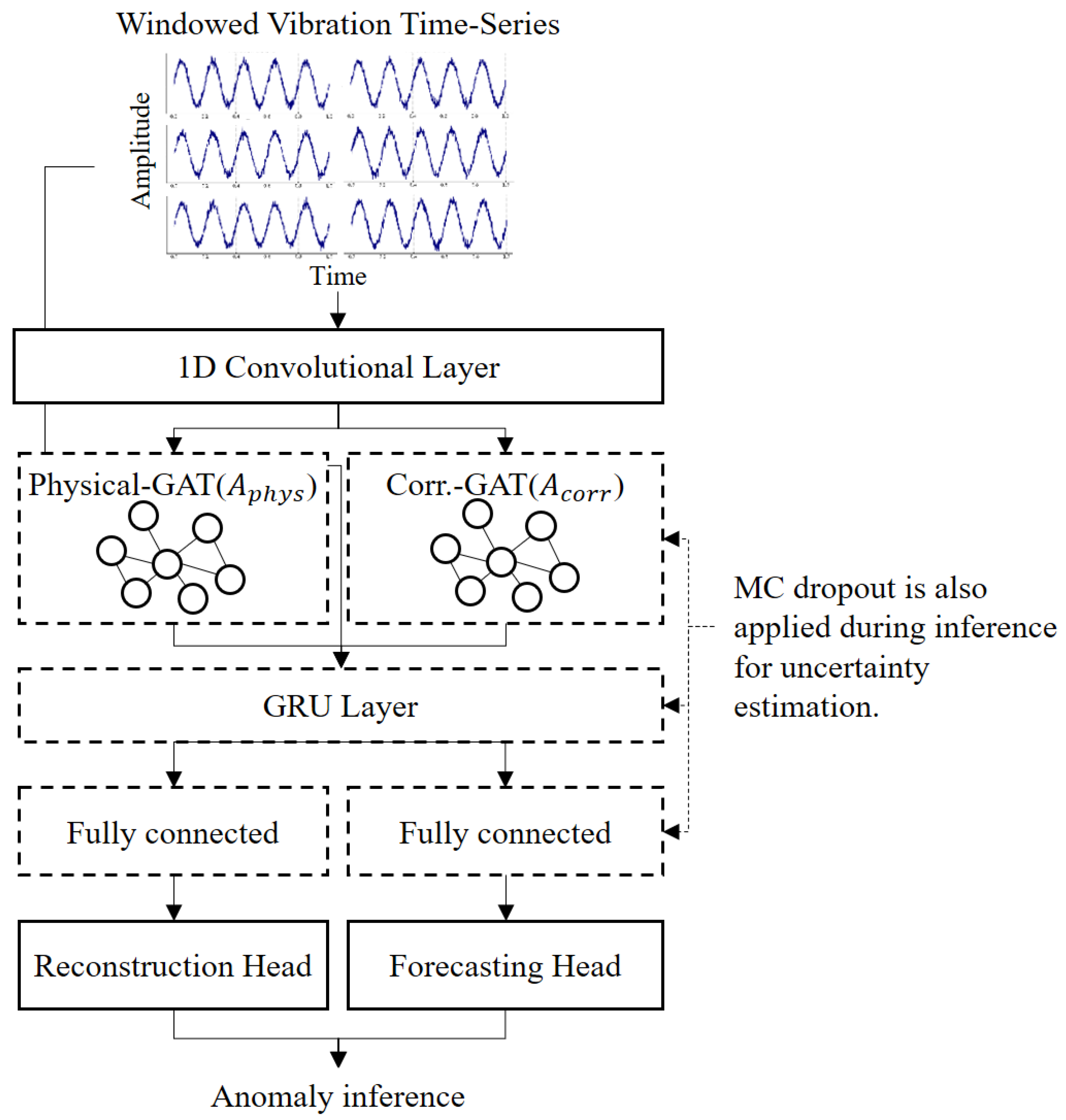
Building on standard deep-learning components for time-series processing, this approach introduces two complementary graph representations (one domain-based and the other data-driven) and a dynamic weighting mechanism for forecasting and reconstruction losses. As illustrated in Figure 1, the revised architecture includes a one-dimensional convolutional feature extractor, dual GAT layers for each graph type, a gated recurrent unit (GRU) for longer-term temporal modeling, and two task-specific output heads (forecasting and reconstruction) connected by an adaptive loss-balancing module. Monte Carlo (MC) dropout is incorporated at multiple layers to capture uncertainty in both tasks. This novel combination provides richer spatiotemporal embeddings, dynamic objective prioritization, and enhanced robustness under uncertain or varying operational conditions.

3.2.1. Dual Graph Construction

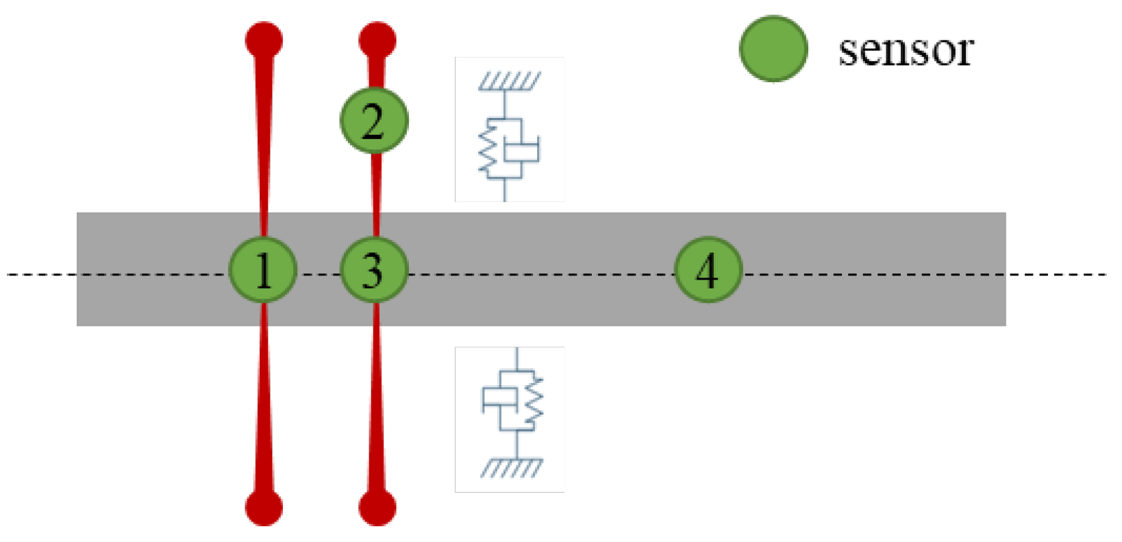
Rotating compressor vibrations often exhibit both physically localized correlations (for example, sensors on the same bearing pedestal) and empirically discovered interdependencies (such as correlated frequency components across distant measurement points). To capture these nuances, the proposed framework maintains two distinct adjacency matrices.
Domain-Informed Adjacency (Aphys): This binary matrix is derived from machine geometry and known couplings (for instance, shared housings or rotor segments). If two sensors i and j lie on physically adjacent components, or on the same rigid body or whose centroidal distance does not exceed 1.5D (shaft diameter), then Aphys (i, j) = 1; otherwise, Aphys (i, j) = 0. Figure 1 illustrates the rule on a four-sensor rotor train. The left bearing block links s 1 and s 3 ( A p h y s 1 , 3 = 1 ). The axial proximity of the over-hung sensor s 2 and s 3 activates A p h y s 2 , 3 = 1 . And the shared shaft segment between s 3 and s 4 gives A p h y s 3 , 4 = 1 . All other pairs remain zero, producing the sparse, block-diagonal pattern in the accompanying adjacency matrix. This design encodes real-world proximity, so the subsequent GAT layer can respect the ways faults propagate through mechanical linkages or shared structural paths.
Data-Correlation Adjacency (Acorr): This matrix is learned from historical or real-time data by computing cross-correlation or mutual information among sensor channels and retaining only those edges that exceed a predefined threshold. It thereby captures relationships that may not be strictly physical, such as resonance-induced couplings or synchronous vibrations that arise under specific load conditions. By maintaining both adjacency matrices, the model exploits first-principle knowledge of machine layout while also incorporating emergent data-driven patterns.

3.2.2. Parallel Dual-Gat Embeddings

Once local vibration features are extracted by one-dimensional convolutions, those features are fed into two parallel GAT layers. One layer operates on Aphys, while the other operates on Acorr. Each GAT layer transforms node features according to
H ( l + 1 ) = σ j N i α i j W h j l
where αij denotes attention coefficients derived from the respective adjacency matrix A, W is a trainable weight matrix, and σ is a nonlinear activation. The attention mechanism redistributes importance among connected nodes, possibly amplifying channels or time steps that are strongly indicative of emerging faults.
The physical graph attention network (Physical-GAT) uses Aphys to emphasize direct mechanical pathways, such as misaligned couplings. The correlation graph attention network (Correlation-GAT) uses Acorr to highlight data-driven relationships, for instance those involving sensor pairs that consistently co-vary under certain operational loads. The outputs of these two GAT layers are then fused, either by concatenation or by an additive scheme, before they are fed into the temporal model. This fusion ensures that the final embedding captures both physically interpretable pathways and latent data associations.

3.2.3. Temporal Modeling with GRU

Although GAT layers can incorporate short-range temporal connections (either through time-oriented edges or within a sliding window), rotating machinery faults may develop gradually or exhibit multi-rotation persistence. Therefore, the fused embeddings are passed to a GRU that processes consecutive windows. The GRU’s hidden state evolves according to
h i = G R U ( z t ,   h t 1 )
where zt is the fused GAT representation at time t. This recurrent mechanism retains a “memory” of how anomalies progress through multiple cycles and changing loads, thereby capturing both near-instantaneous anomalies and longer-term degradations.

3.2.4. Dual-Task Heads with Adaptive Loss Balancing

From the GRU’s final state, the network branches into two heads (Figure 2). The forecasting head predicts near-future vibration samples (for example, one step ahead) and is penalized using the root-mean-square error (RMSE). Sudden deviations in these short-term predictions often indicate emerging faults. The reconstruction head is formulated as an autoencoder-like decoder that reconstructs the entire input window from a latent representation. Large reconstruction errors, measured by the mean squared error (MSE), typically suggest that the observed waveform deviates from normal behavior.
To adaptively prioritize these two objectives, a learnable weighting parameter λ governs the balance between forecasting and reconstruction losses. The overall training loss is
L = λ L f o r e c a s t + ( 1 λ ) L r e c o n
where λ ∈ [0, 1] can be tuned or learned via gradient-based methods. This approach allows the model to shift emphasis depending on whether short-term anomalies (forecasting) or overall waveform fidelity (reconstruction) offers more informative fault indicators. Additionally, skip connections from the fused GAT embeddings to the reconstruction decoder can preserve high-frequency features relevant to sudden events, thereby improving the fidelity of reconstructed signals. The decoder is used only during training. It is dropped at deployment, so the dual-task design does not increase online computational cost. Also, reconstruction of the head provides complementary effects. First, slow or quasi-stationary defects may leave one-step forecasts largely unchanged while progressively distorting a full window; reconstruction error therefore catches faults that the predictor alone can miss. Second, optimizing both heads force the latent representation to preserve short- and long-term information, stabilizing training and sharpening uncertainty estimates.
The Dual-GAT encoder uses four heads for the physical graph and four heads for the correlation graph, each producing 64-dimensional node embeddings. A single-layer GRU with 128 hidden units aggregates the temporal context. Dropout is applied after both the GAT and GRU blocks with a probability of 0.20; during inference, the same rate is kept active for Monte-Carlo sampling. The dual-task loss weight is initialized at λ = 0.50 and learned jointly with the network. Optimization employs Adam optimizer (learning rate 3 × 10 4 , weight decay 1 × 10 2 ) .

3.3. Uncertainty Estimation

Uncertainty estimation is a crucial component of the proposed fault-detection model because it enhances the robustness and reliability of the predictions.
A posterior distribution with two distinct peaks, as shown in Figure 3, highlights this problem; the highest peak, which would be the maximum a posteriori (MAP) estimate, is not representative of the entire distribution—a common problem with MAP estimation; it focuses on the single most likely parameter value, potentially overlooking other significant modes that reflect the underlying uncertainty. By contrast, a Bayesian approach that considers the full posterior distribution provides a more comprehensive picture. By accounting for all possible parameter values and their associated probabilities, the Bayesian approach captures the overall uncertainty and variability within the data, particularly important in cases where the distribution is broad or multimodal because it ensures that the inference is robust and reflective of the true complexity of the parameter space. Therefore, although MAP estimation can be useful for unimodal and narrow distributions, its application to more complex scenarios is limited. The Bayesian approach, which incorporates the entire posterior distribution, offers a richer and more accurate representation of uncertainty, leading to better-informed decision-making.
Bayesian inference enables the measurement of prediction uncertainty. In Bayesian inference, we aim to compute the posterior distribution of the model parameters given the observed data. The posterior distribution provides a probabilistic framework for making predictions, accounting for uncertainty in the model parameters. Mathematically, the posterior distribution is given by Bayes’ theorem:
p θ D ) =   p D θ p ( θ ) p ( D )
where
  • p(θD) is the posterior distribution of the parameters θ given the data D.
  • p(Dθ) is the likelihood of the data given the parameters.
  • p(θ) is the prior distribution of the parameters.
  • p(D) is the marginal likelihood or evidence, computed as shown below.
p D = p D θ p θ d θ
The integral in the denominator, p(D), is practically intractable for complex models because it requires integrating over all possible values of the parameters p(θ). This intractability arises from the high dimensionality of the parameter space and the complexity of the likelihood function, making the exact computation of the posterior distribution computationally infeasible.
The MC dropout, introduced by Gal and Ghahramani [63], provides a method to approximate Bayesian inference in deep neural networks. By incorporating dropouts during both training and inference, we can obtain a distribution of the model predictions. During inference, dropout is applied multiple times to the same input, generating a range of outputs. These outputs are then used to estimate the mean and variance of the predictions, thereby effectively approximating the posterior distribution.
The key idea is to perform multiple stochastic forward passes with dropouts enabled during inference, effectively sampling from the approximate posterior distribution. During training, a dropout is applied to the neurons with a certain probability, p, randomly setting a fraction of the neurons to zero, thus forcing the network to learn redundant representations and preventing overfitting. Mathematically, if h is the hidden layer activation, the dropout modifies it as follows:
h = r     h
where r is a binary mask sampled from a Bernoulli distribution with probability p, and ⊙ denotes element-wise multiplication.
During inference, the dropout remains active, allowing multiple forward passes through the network with different dropout masks. Each forward pass can be viewed as sampling from a different subnetwork, providing a diverse set of predictions. Let y ^ t be the prediction from the t-th forward pass. By performing T such forward passes, we obtain a distribution of predictions.
These approximations allow us to estimate the uncertainty in the predictions of the model without explicitly computing the intractable posterior distribution. Afterward, the types of uncertainty in the model can be determined. Uncertainties in machine learning models can be broadly categorized into aleatoric and epistemic uncertainties. Understanding and quantifying these uncertainties are essential for developing reliable predictive models, particularly for safety-critical applications such as industrial maintenance.
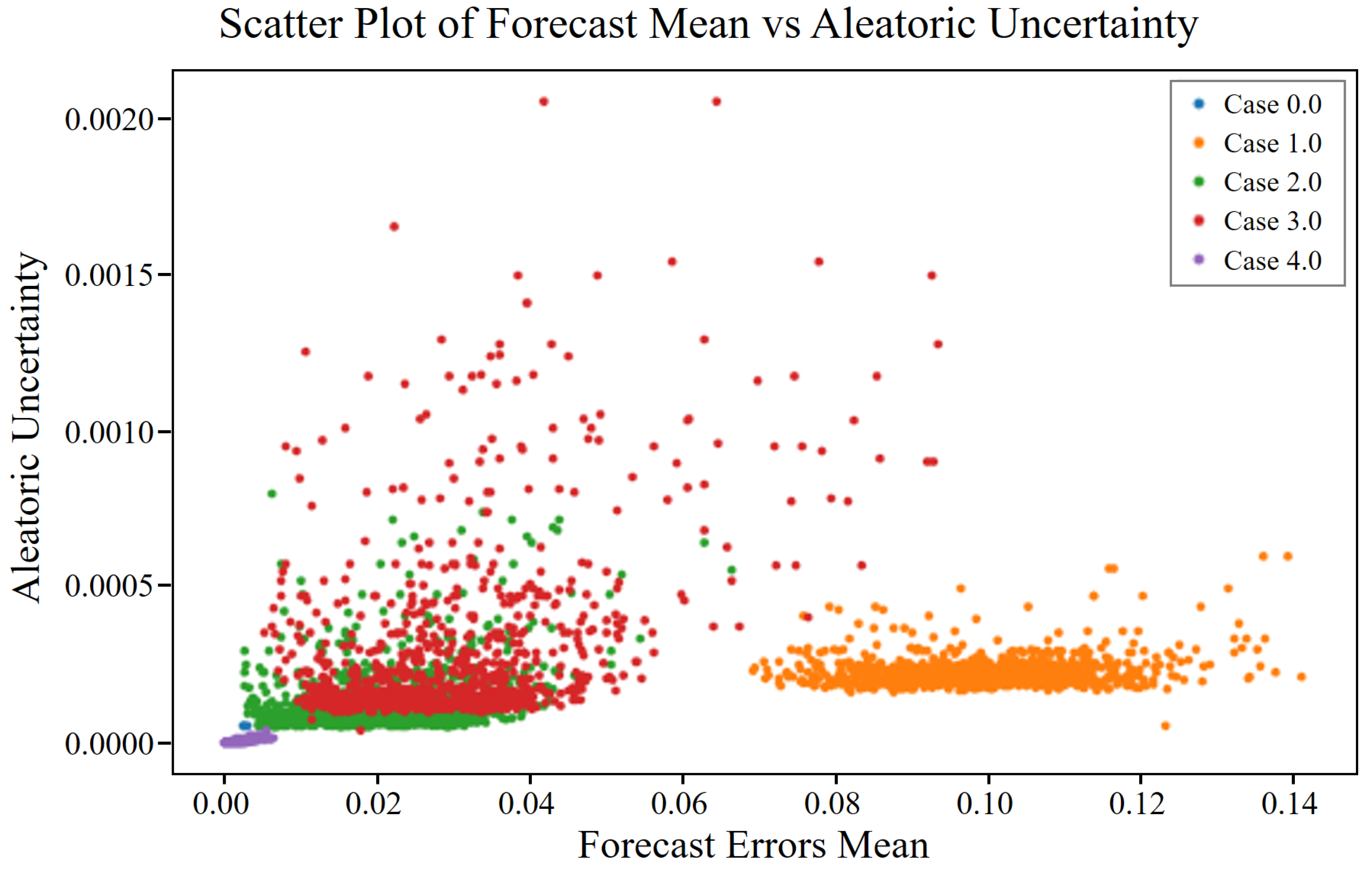
Aleatoric uncertainty, derived from the Latin word “alea”, meaning “dice”, refers to the inherent variability in the data themselves. This type of uncertainty is irreducible and originates from noise inherent in the observations. For example, in compressor vibration data, aleatoric uncertainty may arise from measurement errors owing to sensor precision limits or environmental variations affecting the readings.
Aleatoric Uncertainty :   p y x , θ = N ( y ; f x , θ ,   σ 2 )
Aleatoric uncertainty, often represented as a probabilistic distribution over the output variables, given the input data, can be visualized by plotting confidence intervals around the predictions, indicating regions with high variability due to noise. Notably, increasing the amount of data does not reduce the aleatoric uncertainty because it is intrinsic to the observations.
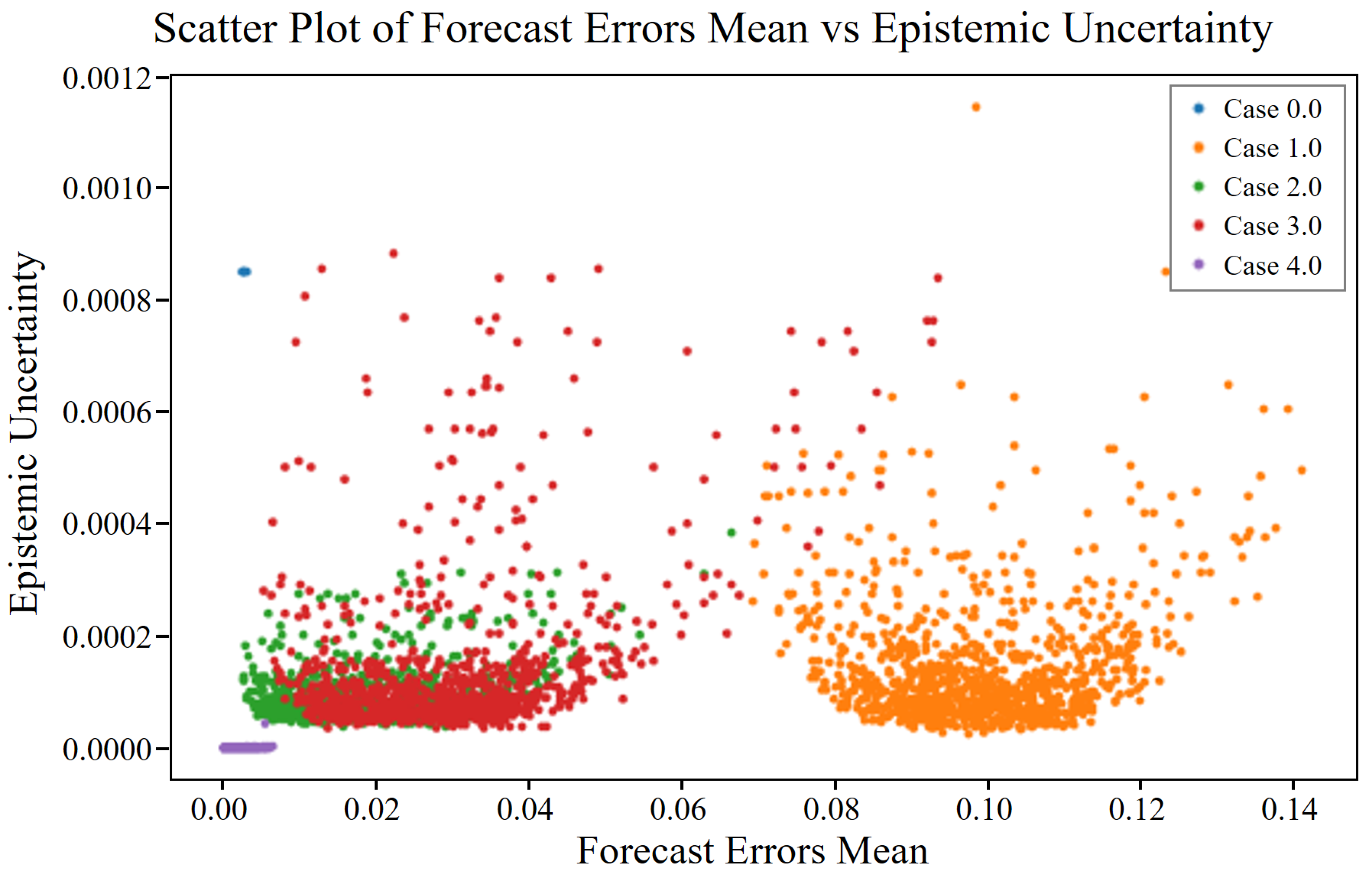
By comparison, epistemic uncertainty, from the Greek word “episteme”, meaning “knowledge”, pertains to uncertainty in the model parameters and structure. This uncertainty is reducible and arises from insufficient training data or a lack of knowledge about the model itself. In the context of compressor vibration data, epistemic uncertainty may be caused by limited data representing certain operational conditions, leading to uncertain predictions in those regions.
Epistemic Uncertainty :   p ( θ | D ) N ( θ ; μ , Σ )
Epistemic uncertainty can be mitigated by acquiring additional data or improving the model, reflecting the confidence of the model in its predictions, based on the knowledge it has gained during training. High epistemic uncertainty often indicates regions where the model has not encountered sufficient similar examples during training, suggesting that further data collection in those areas could improve its performance.
V a r y ^ x , D = E p ( θ | D ) σ 2 x , θ A l e a t o r i c   U n c e r t a i n t y + V a r p ( θ | D ) [ μ x , θ ] E p i s t e m i c   U n c e r t a i n t y
Under a Gaussian weight prior and a Lipschitz feature extractor, the epistemic term scales with the squared Mahalanobis distance from the normal data manifold M 0 ,   i . e . ,   U e p i x | | x μ 0 T 0 1 / 2 | | 2 2 . Because fault severity monotonically increases this distance, epistemic uncertainty also grows monotonically whereas aleatoric uncertainty remains bounded by the intrinsic sensor noise.

3.4. Fault Detection Performance Measurement

To evaluate the performance of the proposed fault-detection model, we conducted extensive experiments on the test dataset, which included both normal and faulty operation data. Analyzing the results of the Bayesian GAT-based fault-detection model from the perspectives of both total loss and uncertainty is essential for a comprehensive evaluation of its performance. Total loss analysis, encompassing forecasting and reconstruction losses, provides an overall measure of the fit of the model to the data. Given that the model was trained solely on normal data, it is expected to produce higher loss values when encountering anomalous data. This difference in loss values can be used to distinguish between normal and faulty conditions. By setting appropriate thresholds for the loss values, we can effectively classify the data as normal or anomalous. Additionally, uncertainty measurements can provide further insights into the degree of confidence of the model in its predictions, indicating how uncertain the model is regarding its classification decisions. Visualizing both the total loss and uncertainties facilitates the understanding of the accuracy of the model and the confidence in its predictions—crucial for decision-making in fault-detection scenarios. Furthermore, comparing these results with those from conventional approaches, such as deterministic GAT or traditional fault-detection methods, underscores the advantages of incorporating Bayesian inference. This comparison demonstrates how the Bayesian GAT model offers a more nuanced understanding of the data through uncertainty quantification, leading to more reliable and informed decisions.

4. Experiments

In this section, the effectiveness of the proposed fault-detection approach is demonstrated using vibration data generated by the digital twin of a compressor in an oil plant. This approach is implemented using PyTorch (2.2.2) and executed on a desktop device equipped with an Intel i9 CPU and four RTX 4090 GPUs

4.1. Fault Detection Performance Measurement

In this study, we developed a digital twin for data generation using the Rotordynamic Open-Source Software (ROSS) to simulate vibration data from a recycle gas compressor at an oil plant. The digital twin encompassed four types of faults: angular misalignment, shaft misalignment, unbalance, and bearing fault. Different analysis conditions were established for these faults considering the analysis direction, fault location, and fault area, as detailed in Table 1. The parameters controlled for each fault type are as follows:
  • Angular misalignment: Degree of misalignment at the coupling and bearing parts of the rotating equipment.
  • Bearing failure: Stiffness value of the bearing part’s oil film.
  • Shaft misalignment: Degree of shaft misalignment.
  • Unbalance: Magnitude of disk unbalance (kg/m).
To align the simulations with classical rotor-dynamics and fault-diagnosis frameworks (e.g., envelope analysis, order tracking), we calibrated the digital twin parameters against representative values reported in established vibration literature. Although this work does not currently include real measured data, the digital twin was validated through cross-checking its natural frequencies and fault signatures with standard rotor-dynamics references to ensure realistic behavior.
Vibration data points were generated for each fault type under various conditions, with an interval of 0.0001 s between points. Transient-state data were generated initially, followed by steady-state data over time. Among the data generated at 0.0001 s intervals from 0 to 5 s, 20,001 data points from the steady-state period between 3 s and 5 s were used. This selection is consistent with standard rotor diagnostic practices, which focus on steady-state data to reduce transient noise and measurement variability. To create fault data, key simulation parameters and causes of faults in the rotating machinery were selected, as mentioned previously. In addition, the material properties of the shaft, disk, and bearings, as defined in Table 2, were incorporated into the simulations. We used only steady-state data because they provide more consistent and reliable information for analyzing and diagnosing faults, thereby reducing the noise and variability inherent in transient-state data.
The digital twin of the compressor, which has been based on the blueprints of an operational recycle gas compressor at an oil plant, is depicted in Figure 4. Detailed positions of the shaft, disk, and bearings were identified for each section of the digital twin of the compressor and turbine, as shown in Figure 5.
Figure 6, which shows an example of data generated using the digital twin, displays six data streams generated from three sensors, with each sensor capturing measurements along the x and y axes.

4.2. Data Preprocessing

As shown in Table 3, which outlines the analysis conditions for types of failure, the raw vibration data exhibited very small mean and standard deviation values on the order of 10−8, and thus, we normalized the data to ensure that all sensor readings were on a comparable scale. This step is essential for avoiding biases during model training, particularly when the features have different units or magnitudes.
Given the time-series nature of the data, we segmented the continuous vibration data into fixed-length sequences. Each sequence represents a window of time over which the sensor readings were analyzed. In this study, after multiple experiments to determine the optimal window size, a window size of 20 was chosen, meaning that each sequence consisted of 20 consecutive data points. In order to set the best window size, a preliminary sensitivity study (validation subset, three random seeds) compared four candidate lengths L = 10 , 20 , 30 , and 40. Inference latency rose roughly linearly from 0.32 ± 0.01 ms per window at L = 10 to 0.95 ± 0.04 ms at L = 40. Classification performance peaked at L = 20, which delivered the highest mean F1-score (0.991) and the best overall metric set (accuracy 0.985, precision 0.990, recall 0.992). Shorter windows (L = 10) suffered a 0.6 drop in F1 score despite their low latency, while longer windows (L = 30, 40) provided no further accuracy benefit yet incurred latencies. Balancing real-time constraints (<0.5 ms) against predictive quality, we therefore fixed L = 20 for all subsequent experiments.
Sliding this window over the 20,001 data points resulted in 19,982 sequences. This window size was selected to balance the tradeoff between capturing sufficient temporal context and maintaining manageable computational complexity.
For each segmented sequence, we constructed a graph to capture both the spatial and temporal dependencies of the sensor readings. The nodes in the graph represent individual sensor measurements, whereas the edges represent the relationships between them. Specifically, we established edges based on known physical relationships and statistical correlations:
  • Nodes corresponding to the same sensor at different timestamps were connected to capture temporal dependencies;
  • Nodes corresponding to different sensors at the same timestamp were connected to capture spatial dependencies;
  • Edges were added based on domain knowledge, such as coupling effects between different components of the compressor.
By following these preprocessing steps, we ensured that the vibration data from the digital twin were adequately prepared for effective fault detection using the GAT model. This comprehensive preprocessing pipeline plays a vital role in the overall success of the anomaly-detection system.
The preprocessed data were split into training, validation, and test sets. For the training set, we used a subset of 2000 sequences of normal data. This selection ensured that the model learned the patterns of normal operations. The remaining data, including both normal and faulty sequences, were then split into validation and test sets. The validation set was used to tune the hyperparameters and prevent overfitting, whereas the test set was used to evaluate the final performance of the model. We ensured that the validation and test sets contained a balanced representation of the different fault types to avoid bias in the learning process of the model.

4.3. Fault Detection Model Training

The fault-detection model training process involves several critical steps to ensure that the GAT effectively learns to detect anomalies in the digital-twin compressor vibration data. The training setup included defining the model architecture, selecting the optimizer, and setting the hyperparameters. As described in Section 3.2, the model architecture consisted of a combination of 1-D convolutional layers, graph attention layers, and a GRU layer, followed by forecasting and reconstruction components. The model was implemented using PyTorch and PyTorch Geometric libraries. The Adam optimizer was selected for its efficiency and adaptive learning rate capabilities, with the initial learning rate set to 0.001. The key hyperparameters included the learning rate, batch size, number of epochs, and dropout rate, with a batch size of 32, training for 100 epochs, and a dropout rate of 0.5, to prevent overfitting.
The training process involved feeding the preprocessed data into the model, calculating the loss, and updating the model parameters using back propagation. The preprocessed training data, consisting of 2000 normal sequences, were loaded and divided into batches. For each batch, the data passed through the 1-D convolutional layer, graph attention layers, and GRU layer, followed by processing through the forecasting and reconstruction components. The total loss was computed as the sum of the forecasting loss and reconstruction loss. The gradients of the loss with respect to the model parameters were computed using back propagation, after which, based on these computed gradients, the Adam optimizer was used to update the model parameters. This process was repeated for each epoch, iterating over all batches in the training dataset until the specified number of epochs was reached or the validation loss plateaued, indicating convergence.
During the training, the validation set was used to measure the performance of the model and tune the hyperparameters. After each epoch, the model was evaluated on the validation set based on metrics such as validation loss and accuracy. To optimize the performance of the model, the hyperparameters were adjusted based on the validation performance using grid search and random search methods. The forecasting loss, reconstruction loss, total loss, and validation loss all decreased over the epochs, as shown in Figure 7.
To assess the performance of the fault-detection model, several evaluation metrics were used, including total loss, forecasting loss, reconstruction loss, and accuracy. These metrics evaluate the ability of the model to correctly identify faults, its sensitivity in detecting all actual faults, and the balance between precision and recall. The final model was selected based on its performance on the validation set, considering these evaluation metrics. The selected model was then evaluated on the test set to assess its generalizability and robustness in detecting faults in previously unseen data.

4.4. Result of Detection

The performance of the proposed Bayesian GAT-based fault-detection model was evaluated and compared against those of an LSTM Autoencoder (LSTM AE)-based reconstruction model and LSTM-based forecasting model. The evaluation was conducted across four types of faults: angular misalignment, bearing failure, shaft misalignment, and unbalance faults. The key performance metrics considered were the accuracy, precision, recall, and F1 score. Table 4 presents the performance metrics for the proposed Bayesian GAT-based anomaly-detection method. The model demonstrated high performance across all fault types, with particularly high precision and recall values. The accuracy and F1 score for each fault type indicate the ability of the model to detect these anomalies accurately and robustly.
Table 5 lists the performance metrics for the LSTM-AE-based reconstruction anomaly-detection method. This method achieved high precision and recall, particularly for shaft faults, with an F1 score of 0.995. However, its performance for bearing faults was comparatively low, with an accuracy of 0.908 and an F1 score of 0.946.
Table 6 lists the performance metrics for the LSTM-based forecasting anomaly-detection method. This method also performed well across all fault types, with high precision and recall. However, the performance was slightly lower than that of the LSTM-AE-based reconstruction method, particularly for angular and bearing faults, for which the accuracies were 0.912 and 0.943, respectively.
Comparing the results across all three methods in Table 7 reveals that the proposed Bayesian GAT-based method provides balanced performance compared to the two methods, especially demonstrating excellent results in terms of precision and recall. These results indicate that the proposed method possesses more reliable and detailed analytical capabilities in defect detection. However, the LSTM-AE-based reconstruction method outperformed the other methods in terms of the overall accuracy and F1 score for angular and shaft faults. Meanwhile, the LSTM-based forecasting method provided a balanced performance, but slightly lagged in accuracy for angular and bearing faults compared to the other two methods.
In summary, whereas each method has its strengths, the Bayesian GAT-based method offers a robust solution with high recall, indicating its reliability in fault detection. Incorporating uncertainty measurements further enhances its applicability in real-world scenarios, where understanding the confidence of a model in its predictions is crucial. By leveraging the advantages of Bayesian inference, the proposed method not only maintains competitive performance, as shown by its metrics, but also provides valuable insights into the uncertainty of its predictions, leading to more reliable and informed decision-making.

4.5. Uncertainty Analysis Result

This subsection presents analysis results for the performance with uncertainty measures, including aleatoric and epistemic, and total uncertainties associated with the forecast and reconstruction errors for different fault cases. To verify that each architectural variant preserves predictive strength while exposing calibrated risk, dropout was kept active during inference ( p = 0.20 ) and N = 30 Monte-Carlo passes were averaged per window. Table 8 reports the mean ± standard deviation of the standard metrics used in Table 5, Table 6 and Table 7, together with the corresponding total uncertainty. The proposed dual-task model sustains the highest classification scores while delivering the largest separation in uncertainty, confirming the complementary value of the reconstruction branch.
To assess the relationship between forecast errors and associated uncertainties, scatter plots were generated as shown in Figure 8, Figure 9 and Figure 10, and data cases were categorized as described in Table 9. Normal data (Case 0) demonstrated low aleatoric and epistemic uncertainties, as shown in Figure 8 and Figure 9, respectively, confirming model robustness under standard conditions. The total uncertainty, illustrated in Figure 10, was correspondingly low. In contrast, fault cases (Cases 1 to 4) exhibited increased uncertainties and forecast errors to varying degrees. Case 3, in particular, showed the highest values across all three figures, indicating a significant challenge for the model in this condition. Notably, Case 1 overlapped visually with Case 0 in the scatter plots, especially in Figure 8, making distinction difficult. Meanwhile, Cases 2 to 4 showed clearer separation in Figure 8, Figure 9 and Figure 10 due to increased noise (aleatoric uncertainty) or reduced parameter confidence (epistemic uncertainty). These findings highlight the usefulness of uncertainty analysis in detecting and distinguishing fault conditions through visualization of different uncertainty types.
To analyze the relationship between reconstruction errors and uncertainties, scatter plots were generated as shown in Figure 11, Figure 12 and Figure 13. Normal data (Case 0) showed very low aleatoric and epistemic uncertainties, as seen in Figure 11 and Figure 12, leading to minimal total uncertainty in Figure 13, which confirms the model’s robustness in reconstructing normal conditions. In contrast, fault cases (Cases 1 to 4) exhibited increased errors and uncertainties to varying degrees. Case 3 showed the highest reconstruction errors and uncertainty levels, indicating significant difficulty for the model under this fault condition. Case 1 showed moderate increases in error and aleatoric uncertainty, while Case 2 presented higher values than Case 1, suggesting increased noise and reduced model confidence. Case 4 demonstrated moderate reconstruction errors and uncertainties, higher than normal but lower than in Cases 2 and 3, indicating relatively better model performance for this fault type.
The analysis of forecast and reconstruction errors along with their associated uncertainties provides a comprehensive understanding of the performance and confidence of the model across different fault types. The clear distinction between normal and fault data in terms of errors and uncertainties underscores the robustness of the model in detecting anomalies. Normal data consistently showed low errors and uncertainties, reflecting high model accuracy and confidence, whereas fault data exhibited higher errors and uncertainties, with the severity of faults correlated with increased noise and decreased confidence in model predictions. These findings validate the effectiveness of the Bayesian GAT-based fault-detection model in identifying anomalies and provide valuable insights into the prediction confidence—crucial for real-world fault-detection scenarios. The ability to quantify both aleatoric and epistemic uncertainties enhances the reliability of the model, making it a robust tool for fault detection and diagnosis in complex systems.
For bearing faults, the scatter plots in Figure 14 and Figure 15 revealed consistent patterns in both forecast and reconstruction errors, as well as in the associated uncertainties. Normal data (Case 0) showed low aleatoric and epistemic uncertainties, indicating stable and confident model performance. As fault severity increased (Cases 1–4), errors and uncertainties also increased across all measures. In Figure 14, related to forecast errors, aleatoric uncertainty increased with severity, with Case 4 showing the highest levels, suggesting significant inherent noise. Epistemic uncertainty also rose sharply in severe faults, indicating reduced model confidence, and total uncertainty peaked in Case 4, combining both factors. Similarly, Figure 15, which presents reconstruction errors, showed increasing aleatoric and epistemic uncertainties with fault severity. Once again, Case 4 exhibited the greatest spread and highest total uncertainty, highlighting the model’s challenge in handling more severe bearing faults.
In the case of shaft misalignment faults, scatter plots were used to examine the relationship between forecast and reconstruction errors and their associated uncertainties. For normal data (Case 0), both aleatoric and epistemic uncertainties were minimal, indicating low inherent noise and high model confidence. As the fault severity increased (Cases 1–4), a wider spread in both errors and uncertainties was observed. According to Figure 16, aleatoric uncertainty in forecast errors increased with fault severity, with Case 4 showing the highest values, suggesting a rise in data noise under more severe conditions. Epistemic uncertainty also rose, indicating decreasing model confidence, and total uncertainty followed the same trend—lowest in normal data and highest in Case 4. Figure 16 also shows that reconstruction errors grew with fault severity, contributing to higher aleatoric uncertainty. In Figure 17, epistemic uncertainty in reconstruction errors increased alongside fault severity, with fault cases—particularly Case 4—exhibiting a wider range of uncertainty. Total uncertainty in reconstruction errors also peaked in Case 4, highlighting the combined effects of increased data noise and reduced model confidence under severe misalignment conditions.
In the case of unbalance faults, similar trends were observed in both forecast and reconstruction errors and their associated uncertainties. Normal data (Case 0) showed minimal aleatoric and epistemic uncertainties, indicating low noise and high model confidence. As the fault severity increased (Cases 1–4), both types of errors and uncertainties also increased. Figure 18 shows that aleatoric uncertainty in forecast errors increased with fault severity, with Case 4 displaying the highest values, reflecting significant inherent noise. Epistemic uncertainty also increased in severe fault cases, suggesting reduced model confidence, and total uncertainty followed the same trend—lowest in normal data and highest in Case 4. In Figure 19, reconstruction errors showed increasing aleatoric and epistemic uncertainties as fault severity rose, with normal data remaining compact and fault cases, particularly Case 4, exhibiting a broader spread. Total uncertainty in reconstruction errors also peaked in Case 4, indicating the combined effect of noise and model uncertainty. These results demonstrate the model’s ability to capture both inherent data variability (aleatoric uncertainty) and confidence in model parameters (epistemic uncertainty), offering a comprehensive understanding of uncertainty across different unbalance fault severities.

5. Conclusions

This paper presents a comprehensive analysis of the performance of a Bayesian GAT-based fault-detection model that considers both conventional performance metrics and uncertainty quantification. On the digital-twin test set, the proposed model attained an overall accuracy of 0.985, precision of 0.990, recall 0.992, and F1 score of 0.991, outperforming both reconstruction-only and forecasting-only baselines. The model therefore consistently distinguishes between normal and faulty conditions, achieving high accuracy, precision, recall, and F1 scores across various fault types, including angular misalignment, axial misalignment, bearing faults, and unbalance faults. Notably, it outperforms conventional reconstruction- and forecasting-error-based approaches, thus demonstrating superior fault-detection capabilities. By incorporating aleatoric and epistemic uncertainties, the proposed framework offers valuable insights into the confidence of its predictions: aleatoric uncertainty reflects the intrinsic noise of the data, whereas epistemic uncertainty indicates the model’s confidence in its parameters. Both types of uncertainty increase with fault severity, indicating that the model is sensitive to the degree of abnormality and revealing heightened challenges in predicting severe faults. By jointly examining forecasting and reconstruction errors with uncertainty measures, this dual-task approach provides a comprehensive view of model performance that accounts for both data-driven noise and model-related uncertainty. The practical implications are significant: the ability to quantify and interpret uncertainties, along with achieving high detection metrics, facilitates more informed decision-making in real-world applications by elucidating the confidence of the model’s outputs. Overall, the Bayesian GAT-based model exhibits robust performance and delivers a detailed perspective on prediction uncertainties, underscoring the importance of incorporating uncertainty quantification to enhance fault-detection reliability and effectiveness. Although the present study is confined to a physics-based digital twin, future work will apply the Bayesian Dual-GAT to field-recorded compressor data as such datasets become available, thereby broadening external validity, and will rigorously evaluate the model’s stability under representative sensor perturbations.
Nonetheless, the absence of real-world experimental validation remains a key limitation, which may affect the model’s direct applicability in practical environments. Accordingly, future research will incorporate actual field data to comprehensively validate the model’s effectiveness and reliability under realistic operating conditions.

Author Contributions

Conceptualization, S.L. and B.J.; methodology, S.L.; software, S.L.; validation, Y.K. and H.-J.C.; resources, Y.K.; writing—original draft preparation, S.L.; writing—review and editing, S.L. and B.J.; visualization, S.L.; supervision, B.J.; project administration, B.J.; funding acquisition, Y.K. All authors have read and agreed to the published version of the manuscript.

Funding

This research was supported by a grant from the Korea Agency for Infrastructure Technology Advancement (KAIA), funded by the Ministry of Land, Infrastructure and Transport (RS-2022-00143644).

Data Availability Statement

The data used in this study are confidential.

Conflicts of Interest

The authors declare that they have no known competing financial interests or personal relationships that could have appeared to influence the work reported in this paper.

References

  1. Marohl, B. 2020 Inflation-Adjusted U.S. Energy Expenditures Lowest Since 2002. Available online: https://www.eia.gov/todayinenergy/detail.php?id=53620 (accessed on 1 June 2025).
  2. World Energy Council. World Energy Resources; World Energy Council: London, UK, 2016. [Google Scholar]
  3. Arsad, A.Z.; Hannan, M.A.; Al-shetwi, A.Q.; Mansur, M.; Muttaqi, K.M.; Dong, Z.Y.; Blaabjerg, F. Hydrogen energy storage intergrated hybrid renewable energy systems: A review analysis for future research directions. Int. J. Hydrog. Energy 2022, 47, 17285–17312. [Google Scholar] [CrossRef]
  4. Bazdar, E.; Sameti, M.; Nasiri, F.; Haghighat, F. Compressed air energy storage in integrated energy systems: A review. Renew. Sustain. Energy Rev. 2022, 167, 112701. [Google Scholar] [CrossRef]
  5. Kurz, R.; Brun, K. Upstream and midstream compression applications: Part 1—Applications. In Proceedings of the ASME Turbo Expo: Power for Land, Sea, and Air, Copenhagen, Denmark, 11–15 July 2012. [Google Scholar]
  6. Priyanka, E.B.; Thangavel, S.; Gao, X.Z. Review analysis on cloud computing based smart grid technology in the oil pipeline sensor network system. Pet. Res. 2020, 6, 77–90. [Google Scholar] [CrossRef]
  7. Boyce, M.P. Gas Turbine Engineering Handbook, 4th ed.; Elsevier: Amsterdam, The Netherlands, 2011. [Google Scholar]
  8. Dawoud, S.M.; Lin, X.; Okba, M.I. Hybrid renewable microgrid optimization techniques: A review. Renew. Sustain. Energy Rev. 2017, 82, 2039–2052. [Google Scholar] [CrossRef]
  9. Jackson, R.B.; Friedlingstein, P.; Quéré, C.L.; Abernethy, S.; Andrew, R.M.; Canadell, J.G.; Ciais, P.; Davis, S.J.; Deng, Z.; Liu, Z.; et al. Global fossil carbon emissions rebound near pre-COVID-19 levels. Environ. Res. Lett. 2022, 17, 031001. [Google Scholar] [CrossRef]
  10. De Castro-Cros, M.; Rosso, S.; Bahilo, E.; Velasco, M.; Angulo, C. Condition Assessment of industrial gas turbine compressor using a drift soft sensor based in Autoencoder. Sensors 2021, 21, 2708. [Google Scholar] [CrossRef] [PubMed]
  11. Han, I.S.; Han, C.; Chung, C.B. Optimization of the air-and gas-supply network of a chemical plant. Chem. Eng. Res. Des. 2004, 82, 1337–1343. [Google Scholar] [CrossRef]
  12. Stevens, P. The role of oil and gas in the economic development of the global economy. Extr. Ind. Soc. 2018, 71, 1–746. [Google Scholar]
  13. Widell, K.N.; Eikevik, T. Reducing power consumption in multi-compressor refrigeration systems. Int. J. Refrig. 2009, 33, 88–94. [Google Scholar] [CrossRef]
  14. Cobos-Zaleta, D.; Ríos-Mercado, R.Z. A MINLP model for minimizing fuel consumption on natural gas pipeline networks. In Proceedings of the XI Latin-Ibero-American Conference on Operations Research, New York, NY, USA, 27–31 October 2002; Springer: Berlin/Heidelberg, Germany, 2002; pp. 90–94. [Google Scholar]
  15. Borraz-Sánchez, C.; Haugland, D. Optimization methods for pipeline transportation of natural gas with variable specific gravity and compressibility. TOP 2011, 21, 524–541. [Google Scholar] [CrossRef]
  16. Kurz, R.; Brun, K. Assessment of Compressors in Gas Storage Applications. J. Eng. Gas Turbines Power 2010, 132, 062402. [Google Scholar] [CrossRef]
  17. Silva, T.L.; Camponogara, E. A computational analysis of multidimensional piecewise-linear models with applications to oil production optimization. Eur. J. Oper. Res. 2013, 232, 630–642. [Google Scholar] [CrossRef]
  18. Inkpen, A.C.; Moffett, M.H. The Global Oil & Gas Industry: Management, Strategy & Finance; PennWell Corporation: Tulsa, OK, USA, 2011. [Google Scholar]
  19. Matania, O.; Dattner, I.; Bortman, J.; Kenett, R.S.; Parmet, Y. A systematic literature review of deep learning for vibration-based fault diagnosis of critical rotating machinery: Limitations and challenges. J. Sound Vib. 2024, 590, 118562. [Google Scholar] [CrossRef]
  20. Khan, A.; Hwang, H.; Kim, H.S. Synthetic data augmentation and deep learning for the fault diagnosis of rotating machines. Mathematics 2021, 9, 2336. [Google Scholar] [CrossRef]
  21. Nandi, S.; Toliyat, H.A.; Li, X. Condition monitoring and fault diagnosis of electrical motors—A review. IEEE Trans. Energy Convers. 2005, 20, 719–729. [Google Scholar] [CrossRef]
  22. Hanga, K.M.; Kovalchuk, Y. Machine learning and multi-agent systems in oil and gas industry applications: A survey. Comput. Sci. Rev. 2019, 34, 100191. [Google Scholar] [CrossRef]
  23. Endrenyi, J.; Aboresheid, S.; Allan, R.N.; Anders, G.J.; Asgarpoor, S.; Billinton, R. The present status of maintenance strategies and the impact of maintenance on reliability. IEEE Trans. Power Syst. 2001, 16, 638–646. [Google Scholar] [CrossRef]
  24. Paté-Cornell, M.E. Learning from the Piper Alpha accident: A postmortem analysis of technical and organizational factors. Risk Anal. 1993, 13, 215–232. [Google Scholar] [CrossRef]
  25. Johnston, R.J. The Role of Oil and Gas Companies in the Energy Transition; Atlantic Council: Washington, DC, USA, 2020. [Google Scholar]
  26. Payne, T. Offshore operations and maintenance: A growing market. Pet. Econ. 2010, 77, 18. [Google Scholar]
  27. Byington, C.S.; Garga, A.K. Data fusion for developing predictive diagnostics for electromechanical systems. In Handbook of Multisensor Data Fusion; CRC Press: Boca Raton, FL, USA, 2017; pp. 721–758. [Google Scholar]
  28. Ahn, G.; Lee, H.; Park, J.; Hur, S. Development of indicator of data sufficiency for feature-based early time series classification with applications of bearing fault diagnosis. Processes 2020, 8, 790. [Google Scholar] [CrossRef]
  29. Kumar, D.; Daudpoto, J.; Harris, N.R.; Hussain, M.; Mehran, S.; Kalwar, I.H.; Hussain, T.; Memon, T.D. The Importance of Feature Processing in Deep-Learning-Based Condition Monitoring of Motors. Math. Probl. Eng. 2021, 2021, 9927151. [Google Scholar] [CrossRef]
  30. Soother, D.K.; Kalwar, I.H.; Hussain, T.; Chowdhry, B.S.; Ujjan, S.M.; Memon, T.D. A Novel Method Based on UNET for Bearing Fault Diagnosis. Comput. Mater. Contin. 2021, 69, 393–408. [Google Scholar] [CrossRef]
  31. Jyothi, R.; Holla, T.; Uma, R.K.; Jayapal, R. Machine learning based multi class fault diagnosis tool for voltage source inverter driven induction motor. Int. J. Power Electron. Drive Syst. 2021, 12, 1205–1215. [Google Scholar] [CrossRef]
  32. Li, T.; Sun, C.; Fink, O.; Yang, Y.; Chen, X.; Yan, R. Filter-informed spectral graph wavelet networks for multiscale feature extraction and intelligent fault diagnosis. IEEE Trans. Cybern. 2023, 54, 506–518. [Google Scholar] [CrossRef]
  33. Wu, X.; Lu, W.; Quan, Y.; Miao, Q.; Sun, P.G. Deep dual graph attention auto-encoder for community detection. Expert Syst. Appl. 2024, 238, 122182. [Google Scholar] [CrossRef]
  34. Zhu, Q.; Zhu, L.; Wang, Z.; Zhang, X.; Li, Q.; Han, Q.; Yang, Z.; Qin, Z. Hybrid triboelectric-piezoelectric nanogenerator assisted intelligent condition monitoring for aero-engine pipeline system. Chem. Eng. J. 2025, 519, 165121. [Google Scholar] [CrossRef]
  35. Le, T.; Le, V. DPFAGA-Dynamic Power Flow Analysis and Fault Characteristics: A Graph Attention Neural Network. arXiv 2025, arXiv:2503.15563. [Google Scholar] [CrossRef]
  36. Shannon, K. Asset Life Cycle Management Optimizes Performance American Oil Gas Reporter 2012. Available online: https://www.aogr.com/web-exclusives/exclusive-story/asset-life-cycle-management-optimizes-performance (accessed on 1 June 2025).
  37. Jia, M.; Du, R. Fault diagnosing of large rotating machinery using evolutionary spectrum. In Proceedings of the ASME 1998 International Mechanical Engineering Congress and Exposition, Anaheim, CA, USA, 15–20 November 1998. [Google Scholar]
  38. Chen, Y.D.; Du, R.; Qu, L.S. Fault features of large rotating machinery and diagnosis using sensor fusion. J. Sound Vib. 1995, 188, 227–242. [Google Scholar] [CrossRef]
  39. Hmida, F.B.; Khémiri, K.; Ragot, J.; Gossa, M. Three-stage Kalman filter for state and fault estimation of linear stochastic systems with unknown inputs. J. Frankl. Inst. 2012, 349, 2369–2388. [Google Scholar] [CrossRef]
  40. Capisani, L.M.; Ferrara, A.; De Loza, A.F.; Fridman, L.M. Manipulator fault diagnosis via higher order sliding-mode observers. IEEE Trans. Ind. Electron. 2012, 59, 3979–3986. [Google Scholar] [CrossRef]
  41. Salmasi, F.R.; Najafabadi, T.A.; Maralani, P.J. An adaptive flux observer with online estimation of DC-link voltage and rotor resistance for VSI-based induction motors. IEEE Trans. Power Electron. 2010, 25, 1310–1319. [Google Scholar] [CrossRef]
  42. Isermann, R. Model-based fault-detection and diagnosis–status and applications. Annu. Rev. Control 2005, 29, 71–85. [Google Scholar] [CrossRef]
  43. Patton, R.J.; Chen, J. Observer-based fault detection and isolation: Robustness and applications. Control Eng. Pract. 1997, 5, 671–682. [Google Scholar] [CrossRef]
  44. Ozbek, M.; Soffker, D. Feature-Based Fault Detection Approaches. In Proceedings of the 2006 IEEE International Conference on Mechatronics (ICMECH), Budapest, Hungary, 3–5 July 2006. [Google Scholar] [CrossRef]
  45. Cheng, G.; Cheng, Y.L.; Shen, L.H.; Qiu, J.B.; Zhang, S. Gear fault identification based on Hilbert–Huang transform and SOM neural network. Measurement 2012, 46, 1137–1146. [Google Scholar] [CrossRef]
  46. Mahgoun, H.; Bekka, R.E.; Felkaoui, A. Gearbox fault detection using a new denoising method based on ensemble empirical mode decomposition and FFT. In Proceedings of the 4th International Conference Integrity, Reliability and Failure (IRF), Funchal, Portugal, 21–25 July 2013; pp. 1–11. [Google Scholar]
  47. Haddad, R.Z.; Strangas, E.G. On the accuracy of fault detection and separation in permanent magnet synchronous machines using MCSA/MVSA and LDA. IEEE Trans. Energy Convers. 2016, 31, 924–934. [Google Scholar] [CrossRef]
  48. Camarena-Martinez, D.; Osornio-Rios, R.; Romero-Troncoso, R.J.; Garcia-Perez, A. Fused empirical mode decomposition and MUSIC algorithms for detecting multiple combined faults in induction motors. J. Appl. Res. Technol. 2015, 13, 160–167. [Google Scholar] [CrossRef]
  49. Wang, G.; Liu, C.; Cui, Y. Clustering diagnosis of rolling element bearing fault based on integrated Autoregressive/Autoregressive Conditional Heteroscedasticity model. J. Sound Vib. 2012, 331, 4379–4387. [Google Scholar] [CrossRef]
  50. Mack, D.L.C.; Biswas, G.; Khorasgani, H.; Mylaraswamy, D.B.; Haradwaj, R. Combining expert knowledge and unsupervised learning techniques for anomaly detection in aircraft flight data. At-Autom. 2018, 66, 291–307. [Google Scholar] [CrossRef]
  51. Amruthnath, N.; Gupta, T. A research study on unsupervised machine learning algorithms for early fault detection in predictive maintenance. In Proceedings of the 5th International Conference on Industrial Engineering and Applications (ICIEA), Singapore, 26–27 April 2018. [Google Scholar] [CrossRef]
  52. Tharrault, Y.; Mourot, G.; Ragot, J. Fault detection and isolation with robust principal component analysis. In Proceedings of the 16th Mediterranean Conference Control Automation (MED), Ajaccio, France, 25–27 June 2008. [Google Scholar] [CrossRef]
  53. Sree, A.; Venkata, K. Anomaly detection using principal component analysis. J. Computer. Sci. Technol. 2014, 5, 124–126. [Google Scholar]
  54. Li, Y.; Yang, Y.; Wang, X.; Liu, B.; Liang, X. Early fault diagnosis of rolling bearings based on hierarchical symbol dynamic entropy and binary tree support vector machine. J. Sound Vib. 2018, 428, 72–86. [Google Scholar] [CrossRef]
  55. Galbraith, K.; Alaca, O.; Ekti, A.R.; Wilson, A.; Snyder, I.; Stenvig, N.M. On the investigation of phase fault classification in power grid signals: A case study for support vector machines, decision tree and random forest. In Proceedings of the 2023 North American Power Symposium (NAPS), College Station, TX, USA, 15–17 October 2023; IEEE: New York, NY, USA, 2023; pp. 1–6. [Google Scholar]
  56. Perumal, S.K.; Meenakshi, S. Intelligent machine fault detection in industries using supervised machine learning techniques. In Proceedings of the 2023 International Conference on Data Science, Agents & Artificial Intelligence (ICDSAAI), Chennai, India, 20–22 September 2023; IEEE: New York, NY, USA, 2023; pp. 1–5. [Google Scholar]
  57. Wen, L.; Li, X.; Gao, L.; Zhang, Y. A new convolutional neural network-based data-driven fault diagnosis method. IEEE Trans. Ind. Electron. 2017, 65, 5990–5998. [Google Scholar] [CrossRef]
  58. Zhang, Y.; Zhou, T.; Huang, X.; Cao, L.; Zhou, Q. Fault diagnosis of rotating machinery based on recurrent neural networks. Measurement 2021, 171, 108774. [Google Scholar] [CrossRef]
  59. Huang, T.; Zhang, Q.; Tang, X.; Zhao, S.; Lu, X. A novel fault diagnosis method based on CNN and LSTM and its application in fault diagnosis for complex systems. Artif. Intell. Rev. 2022, 55, 1289–1315. [Google Scholar] [CrossRef]
  60. Yan, K.; Su, J.; Huang, J.; Mo, Y. Chiller fault diagnosis based on VAE-enabled generative adversarial networks. IEEE Trans. Autom. Sci. Eng. 2020, 19, 387–395. [Google Scholar] [CrossRef]
  61. Hu, Z.; Han, T.; Bian, J.; Wang, Z.; Cheng, L.; Zhang, W.; Kong, X. A deep feature extraction approach for bearing fault diagnosis based on multi-scale convolutional autoencoder and generative adversarial networks. Meas. Sci. Technol. 2022, 33, 065013. [Google Scholar] [CrossRef]
  62. Zhao, H.; Wang, Y.; Duan, J.; Huang, C.; Cao, D.; Tong, Y.; Xu, B.; Bai, J.; Tong, J.; Zhang, Q. Multivariate time-series anomaly detection via graph attention network. In Proceedings of the 2020 IEEE International Conference on Data Mining (ICDM), Sorrento, Italy, 17–20 November 2020; IEEE: New York, NY, USA, 2020; pp. 841–850. [Google Scholar]
  63. Gal, Y.; Ghahramani, Z. Dropout as a bayesian approximation: Representing model uncertainty in deep learning. In Proceedings of the International Conference on Machine Learning, New York City, NY, USA, 19–24 June 2016; PMLR: New York, NY, USA, 2016; pp. 1050–1059. [Google Scholar]
Figure 1. Examples of rotor layout with adjacency matrix A p h y s 1 , 3 = 1 ,     A p h y s 2 , 3 = 1 ,   A p h y s 3 , 4 = 1 .
Machines 13 00673 g001
Figure 2. Proposed architecture, including MC dropout for uncertainty estimation.
Machines 13 00673 g002
Figure 3. Illustration of multimodal posterior distribution.
Machines 13 00673 g003
Figure 4. Simplified schematic representation of rotary machine, emphasizing its key components: compressor and turbine. Diagram was streamlined to safeguard proprietary information.
Machines 13 00673 g004
Figure 5. Modeling result.
Machines 13 00673 g005
Figure 6. Examples of generated data from digital twin.
Machines 13 00673 g006
Figure 7. Training and validation loss over epochs.
Machines 13 00673 g007
Figure 8. Aleatoric uncertainty vs. mean forecast error for different cases of angular misalignment fault.
Machines 13 00673 g008
Figure 9. Epistemic uncertainty vs. mean forecast error for different cases of angular misalignment fault.
Machines 13 00673 g009
Figure 10. Total uncertainty vs. mean forecast error for different cases of angular misalignment fault.
Machines 13 00673 g010
Figure 11. Aleatoric uncertainty vs. mean reconstruction error for different cases of angular misalignment fault.
Machines 13 00673 g011
Figure 12. Epistemic uncertainty vs. mean reconstruction error for different cases of angular misalignment fault.
Machines 13 00673 g012
Figure 13. Total uncertainty vs. mean reconstruction error for different cases of angular misalignment fault.
Machines 13 00673 g013
Figure 14. Total uncertainty vs. mean forecast error for different cases of bearing fault.
Machines 13 00673 g014
Figure 15. Total uncertainty vs. mean reconstruction error for different cases of bearing fault.
Machines 13 00673 g015
Figure 16. Total uncertainty vs. mean forecast error for different cases of shaft misalignment fault.
Machines 13 00673 g016
Figure 17. Total uncertainty vs. mean reconstruction error for different cases of shaft misalignment fault.
Machines 13 00673 g017
Figure 18. Total uncertainty vs. mean forecast error for different cases of unbalance fault.
Machines 13 00673 g018
Figure 19. Aleatoric uncertainty vs. mean reconstruction error for different cases of unbalance fault.
Machines 13 00673 g019
Table 1. Mean (standard deviation) of accuracy of proposed model and baseline models.
Fault TypeFault CauseKey Factors of Simulation
Angular misalignmentShaft axis tilted (bearing issue)Angle deviation (°)
Bearing failureWear, poor lubrication, heatWear, lubrication, temperature
Shaft misalignmentShaft axis laterally offsetx- and y-offset (mm)
UnbalanceMass center off rotation centerImbalance magnitude
Table 2. Material property settings.
MaterialPropertiesValue
Angular misalignmentDensity (kg/m3)7850
Young’s modulus (GPa)217
Shear modulus (GPa)81.2
Poisson coefficient0.299
DiskMass (kg)2.6375
Polar moment of inertia (kg·m2)0.0075
Diametral moment of inertia (kg·m2)0.003844
BearingX-direction stiffness (N/m)950
Y-direction stiffness (N/m)109,000
Damping coefficient (N·s/m)50.4
Table 3. Analysis conditions for types of failure.
CategoryDisplacement Direction (x,y)Number of Parameters
Angular misalignment210
Bearing failure25
Shaft misalignment210
Unbalance misalignment25
Table 4. Performance metrics of proposed anomaly-detection method.
Fault TypeAccuracyPrecisionRecallF1 Score
Angular misalignment0.8650.9940.8540.919
Bearing failure0.9920.9901.0000.995
Shaft misalignment0.9950.9951.0000.997
Unbalance0.9920.9901.0000.995
Table 5. Performance metrics of reconstruction-error-based anomaly-detection method.
Fault TypeAccuracyPrecisionRecallF1 Score
Angular misalignment0.9700.9671.0000.983
Bearing failure0.9080.8981.0000.946
Shaft misalignment0.9920.9911.0000.995
Unbalance0.9530.9451.0000.972
Table 6. Performance metrics of forecasting-error-based anomaly-detection method.
Fault TypeAccuracyPrecisionRecallF1 Score
Angular misalignment0.9120.9120.9890.950
Bearing failure0.9430.9311.0000.964
Shaft misalignment0.9470.9421.0000.970
Unbalance0.9250.9111.0000.953
Table 7. Comparative performance metrics of anomaly-detection methods.
MethodAccuracyPrecisionRecallF1 Score
Proposed0.9850.9900.9920.991
Reconstruction based0.9550.9501.0000.974
Forecasting based0.9310.9240.9970.959
Table 8. Comparative performance metrics of anomaly-detection methods with MC dropout (mean ±   1 σ ).
MethodAccuracyPrecisionRecallF1 Score
Proposed0.985 ± 0.0040.990 ± 0.0050.992 ± 0.0040.991 ± 0.004
Reconstruction based0.960 ± 0.0050.951 ± 0.0070.978 ± 0.0060.964 ± 0.006
Forecasting based0.957 ± 0.0060.962 ± 0.0080.948 ± 0.0070.955 ± 0.007
Table 9. Comparative performance metrics of anomaly-detection methods by case.
CategoryParameter
Case 1Case 2Case 3Case 4
Angular misalignment0.1°0.2°0.3°0.4°
Bearing failure1 × 1081 × 108 × (0.6)11 × 108 × (0.6)21 × 108 × (0.6)3
Shaft misalignment2 × 10−42 × 10−4 × (0.6)12 × 10−4 × (0.6)22 × 10−4 × (0.6)3
Unbalance misalignment5 × 10−45 × 10−4 × (0.3)15 × 10−4 × (0.3)25 × 10−4 × (0.3)3
Disclaimer/Publisher’s Note: The statements, opinions and data contained in all publications are solely those of the individual author(s) and contributor(s) and not of MDPI and/or the editor(s). MDPI and/or the editor(s) disclaim responsibility for any injury to people or property resulting from any ideas, methods, instructions or products referred to in the content.

