1. Introduction
According to their kinematic structure, robot manipulators can be divided into two categories: open-kinematic chain mechanism (OKCM) manipulators and closed-kinematic chain mechanism (CKCM) manipulators [
1]. OKCM manipulators consist of a series of links interconnected by joints and extend from a base to an end-effector. This type of manipulator has a long reach and a large workspace. However, it has several disadvantages, such as low rigidity and poor performance at high speed and high loading conditions. CKCM manipulators, also well known as parallel manipulators, in general consist of a moving platform and a fixed base platform interconnected by several links. In these manipulators, all links act in a parallel manner and share the same payload. Therefore, they can improve their tracking performance by avoiding accumulated and amplified errors from link to link [
2,
3,
4], as occur in the case of OKCM manipulators. As a result, they are superior to OKCM manipulators in applications that require high force/torque capability, high position accuracy, fast motion, and large payload-carrying capacity in a relatively small workspace for tasks including arc welding, cutting, sealing, medical rehabilitation, high-speed assembly operation, and microchip assembly operation [
3,
4,
5,
6].
Despite the advantages presented above, the complexity of the dynamical model and the closed-kinematic structure of CKCM manipulators make the development of controllers for motion control very challenging. Control schemes developed for CKCM manipulators can be classified into two main groups, namely model-based and performance-based methods [
7]. Model-based control methods such as the computed torque method [
8] require precise manipulator dynamics in their control law formulation. Consequently, the performance of these control methods can be deteriorated due to imprecise mathematical manipulator models. In addition, the implementation of model-based control schemes is computationally intensive due to the required computation of complicated manipulator dynamics. On the other hand, performance-based control schemes such as adaptive control techniques do not need the complex mathematical model of manipulator dynamics in their control law formulation. As a result, these control schemes are very computationally efficient and suitable for real-time applications. One of the well-known adaptive control techniques is model reference adaptive control (MRAC) [
9], the main idea of which is to obtain a closed-loop system with adjustable controller parameters capable of changing the behavior of the closed-loop system. The main purpose of MRAC is to force the controlled system to act like a desired reference model to effectively deal with uncertainties and changes in the system or its environment [
10]. While numerous MRAC-based control schemes have been developed for OKCM manipulators [
11,
12], only a few control schemes have been proposed for CKCM manipulators. In [
13], an MRAC-based adaptive control scheme was developed for motion control of a 6-DOF parallel manipulator built as a prototype to study in space operations such as robotic maintenance and repair of spacecrafts. This developed adaptive control scheme included a proportional-derivative (PD) feedback controller with gains adjusted by an adaptation law. Using the Lyapunov direct method, the authors derived an adaptation law that stabilized the error dynamics. Furthermore, neural networks were employed to control the motion of parallel robot manipulators. A decentralized proportional integral derivative (PID) controller in Cartesian space was enhanced by an artificial neural network to improve the tracking performance of a 2-DOF redundant parallel manipulator [
14].
Unlike OKCM manipulators, one unique property of CKCM manipulators is that due to their closed-kinematic structure, the motion of each of their active joints is affected by that of other active joints. However, in most conventional controllers for CKCM manipulators, the control loops of the actuators do not communicate with each other, and as a result, each control loop only handles errors of its own actuator regardless of those of other actuators. Thus, synchronization among actuators is needed to avoid a reduction in motion control performance. In addition, because the actuators of CKCM manipulators are arranged in parallel, the lack of synchronization might produce large interactional forces, which in turn could wear out the actuators prematurely. In the search for a solution for the above synchronization issue, the cross coupling control method came up as a potential candidate. A synchronization technique based on the concept of cross coupling control was designed to tackle the above issue by letting each control loop receive feedback from itself as well as from the others to achieve better coordination and improve the manipulator performance significantly [
15]. Other studies considering cross coupling errors to improve the synchronization performance of two-axis motions can be found in [
16,
17,
18]. Synchronized control schemes with control law implementation that do not require knowledge of the manipulator dynamics were developed by researchers in [
19,
20,
21]. Recently, researchers in [
22] developed a new adaptive control scheme for CKCM robot manipulators, which combined both the concepts of synchronization control and MRAC, called the decentralized adaptive synchronized control scheme (DASCS). In [
22], computer simulation results obtained showed that the DASCS had the ability to effectively control a 6-DOF CKCM manipulator without knowledge of the manipulator dynamics and thus was suitable for real-time implementation. Focusing on the experimental aspect of the DASCS, the present paper will report and discuss results of real-time experiments conducted to evaluate the performance of the DASCS in comparison with that of a traditional MRAC scheme developed by Seraji in [
7], namely the SMRACS. The specific contributions of the present paper include an experimental investigation of the effectiveness of the DASCS for a 2-DOF CKCM manipulator and an experimental evaluation of its control performance in comparison to that of a traditional adaptive control scheme, namely SMRACS. Furthermore, this study experimentally proves that the incorporation of synchronized control into an adaptive control scheme enhances the control performance of the original control scheme when applied to control CKCM manipulators.
The present paper is organized as follows:
Section 2 describes the testbed employed in our experimental investigation of the DASCS.
Section 3 gives an overview of the development of the DASCS consisting of the synchronization control method and the MRAC method.
Section 4 presents and discusses the results of real-time experiments conducted to evaluate the control performance of the DASCS in comparison with the SMRACS.
Section 5 concludes the paper with a summary of the study and recommendations for future research.
2. The Control Scheme Testbed
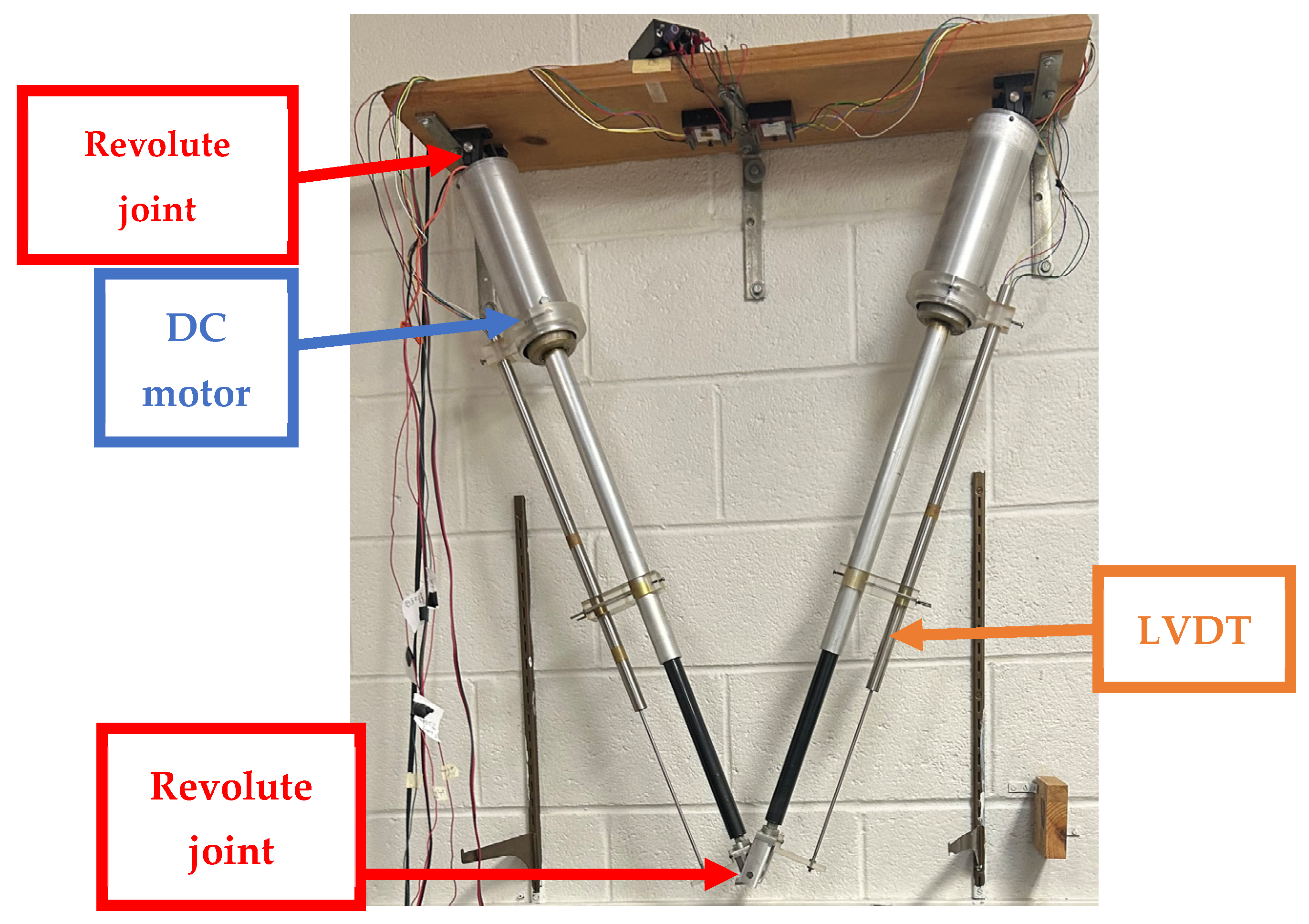
The testbed used to evaluate the control performance of the DASCS consisted of a real CKCM robot manipulator possessing two DOFs (
Figure 1) [
23] and its closed-loop control system (
Figure 2). This manipulator was designed and built to prove a proposed concept implying that CKCM robot manipulators were capable of performing high-precision motions for potential space applications such as assembling and maintaining NASA spacecrafts.
Figure 1 shows that the manipulator is composed of two links, each of which consists of a ball screw linear actuator activated by a DC motor. Two pin joints acting as revolute joints mount the top end of each link under a fixed platform. The same type of revolute joints are used to couple the other ends of the links, on which a tool can be mounted to carry out robotic tasks. The actual lengths of the two actuators are measured by two linear voltage differential transformers (LVDTs) mounted along the links. The LVDTs serve as joint position sensors to provide real-time information on actual link lengths for feedback control.
Table 1 contains the specifications of the ball screw actuators and the manipulator parameters, and
Table 2 contains the specifications of the LVDTs.
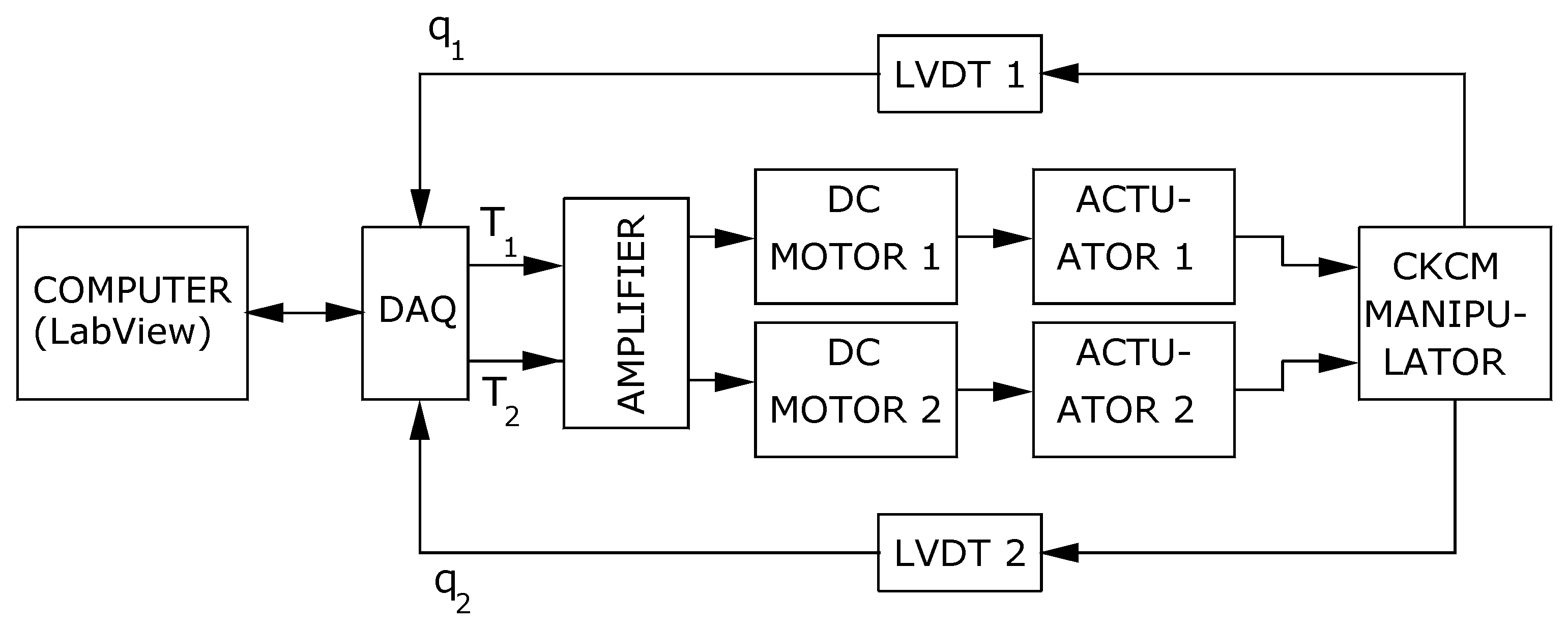
The control scheme testbed is presented in a block diagram in
Figure 2, where a data acquisition system (DAQ) serves as an interface between a computer and the outside world composed of the manipulator, LVDTs as sensors, and the actuator drivers. LabView version 2019, which is a graphical programming environment, allows for data acquisition and analysis to be performed in real time. As illustrated in
Figure 3, the two LVDTs provide real-time information on the manipulator lengths as joint variables q
1(t) and q
2(t), which are fed to the DAQ. The DAQ provides joint variables q
1(t) and q
2(t) to LabView, which in turn carries out all necessary computation for the DASCS. The DAQ then takes T
1(t) and T
2(t), computed by the DASCS adaptation law as developed in
Section 2 below, and sends them to the respective DC motors and actuators. T
1(t) and T
2(t), which are low-level control signals expressed in DC voltages (in mV), are sent to a DC amplifier, which in turn amplifies the signals to higher-level DC voltages (from −24 V to +24 V) to reach an appropriate voltage level to activate the DC motors.
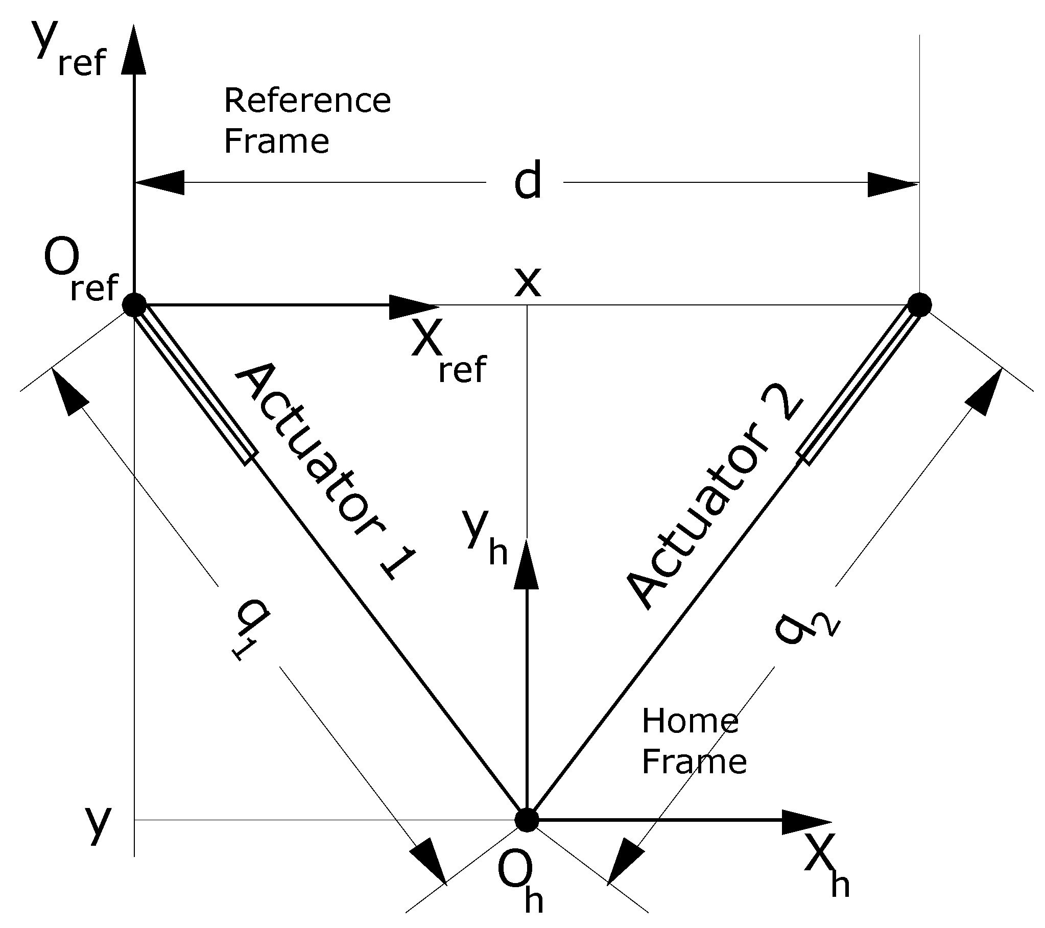
Figure 3 shows the frame assignment of the manipulator, where the lengths of its links,
and
(t), are denoted as its joint variables. A fixed Reference Frame {X
ref, Y
ref, O
ref} is assigned using the right-hand rule so that its origin O
ref coincides with the revolute joint of Actuator 1; X
ref-Axis aligns with the revolute joints of Actuator 1 and Actuator 2, and Y
ref-Axis is perpendicular to X
ref-Axis. The variables x(t) and y(t), representing the horizontal and vertical positions of the manipulator end-effector with respect to the Reference Frame, respectively, are the Cartesian variables of the manipulator. In addition, a fixed Home Frame {X
h, Y
h, O
h} is assigned using the right-hand rule so that its origin O
h is at the center of the robot end-effector when the manipulator is in the home position. We note that the X
h-Axis and the Y
h-Axis of the Home Frame are parallel to the X
ref-Axis and the Y
ref-Axis of the Reference Frame, respectively. Any position in the Home Frame can be transformed to the Reference Frame by a fixed homogeneous transformation. The Home Frame will be used in the next section to represent the data collected by LabView via the DAQ.
We proceed to derive kinematic solutions for the manipulator. From
Figure 3, the joint variables
and
of Actuator 1 and Actuator 2, respectively, can be computed from the Cartesian variables
x(
t) and
y(
t) by
and
where d is the distance between the top ends of the links, which are at the centers of the pin joints suspending the two actuators.
By definition, Equations (1) and (2) provide a closed-form solution for the manipulator inverse kinematics, meaning that they can be used to calculate the joint variables and from the Cartesian variables x(t) and y(t).
In addition, from Equations (1) and (2), the Cartesian variables
x(t) and
y(t) can be derived as follows:
By definition, Equations (3) and (4) represent a closed-form solution of the manipulator forward kinematics, allowing the determination of the Cartesian variables x(t) and y(t) from the joint variables and .
3. Overview of the DASCS
The complete and detailed development of the DASCS can be found in [
22]. Since this paper focuses on the experimental evaluation of the above control scheme, this section contains only relevant mathematical expressions and equations for the adaptive control law of the developed control scheme. From [
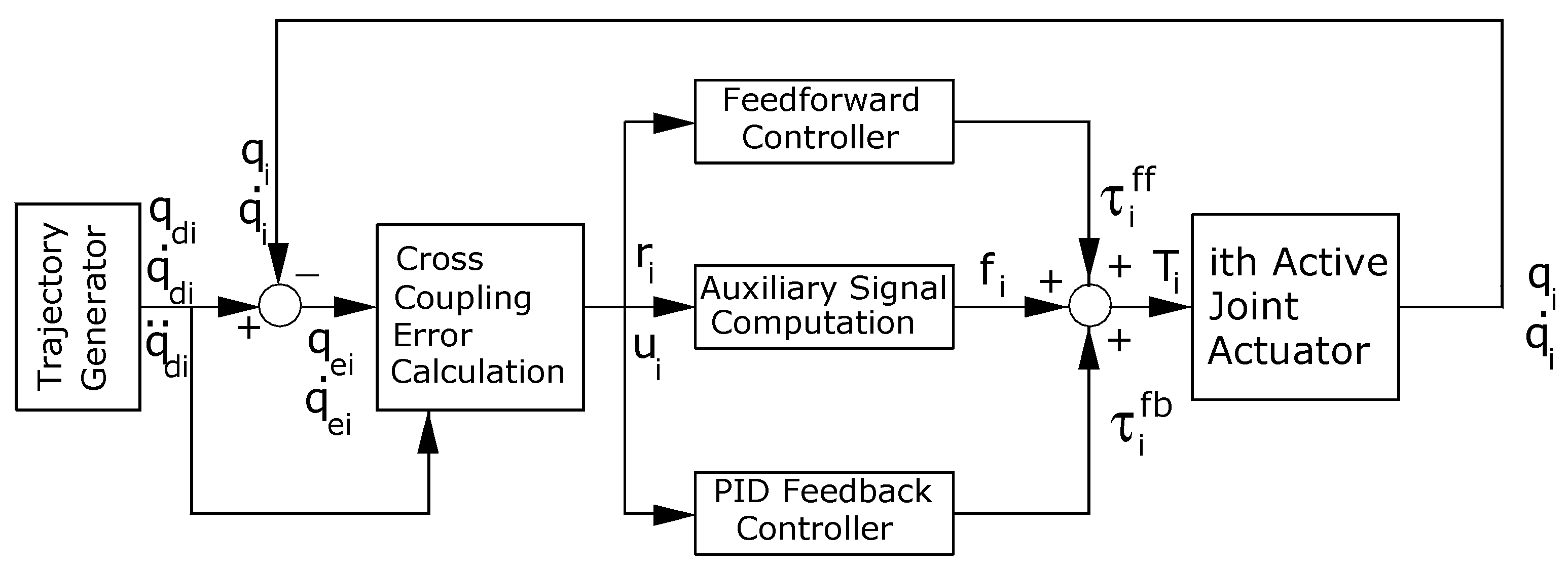
22], a block diagram of the DASCS with its controllers is presented in
Figure 4, where each
ith active joint of the above manipulator is controlled by a separate controller in a decentralized structure. The joint variable error
is computed as
where
and
denote the desired and actual time trajectory of the
active joint, respectively. The Cross Coupling Error Calculation Block calculates the command signal
as
and generates the generalized error
as
where the cross coupling error
is determined by
and the synchronization error
is given by
where
.
From [
22], the control signal
that is sent to the
ith joint actuator is given by
We see that , representing the adaptive control law, is composed of three terms:
The first term , produced by the Auxiliary Signal Computation Block represents the auxiliary signal to partly compensate for disturbance and to improve tracking performance.
The second term = represents the PID feedback controller. This term is generated by the PID Feedback Controller Block.
The last term represents the feedforward controller and is computed by the Feedforward Controller Block.
Various functions and parameters of the above terms can be determined by
where
are positive constants and
are zero or positive constants;
where
and
are positive constants. Furthermore,
(0),
(0),
(0),
(0),
, and
, which are the initial conditions of
,
,
,
,
, and
, respectively, can be set arbitrarily. We note that in (11), the subindex
i was dropped for presentation simplicity. It is noted that
, as seen in Equation (10), was a result of applying the Lyapunov direct method in the development of the DASCS and thus ensuring asymptotic stability of the closed-loop feedback control system.
As seen in
Figure 4, the desired position, velocity, and acceleration of the active joint, which are generated by the Trajectory Generator, are the required inputs of the ith controller. In addition, the actual positions and velocities of its active joint and of the two adjacent ones are the required measurements for feedback control.
Since the results of experiments conducted to evaluate the performance of the DASCS in comparison to that of SMRACS will be presented and discussed in the next section, it is pertinent now to give an overview of the above control schemes to highlight their differences. Detailed development of the control schemes can be found in [
22] for the DASCS and in [
7] for the SMRACS. Motivated to alleviate the disadvantages of model-based control techniques, including the heavy computational requirements of manipulator dynamics, reliance on the fidelity of manipulator models, and non-suitability for real-time applications, Seraji in [
7] developed an adaptive control scheme, namely the SMRACS, for OKCM manipulators. The development of the SMRACS was based on the concept of MRAC [
9], and the Lypunov direct method was employed to ensure the stability of this control scheme. However, being intended for motion control of OKCM manipulators, the SMRACS lacks the synchronized control of active joints of CKCM manipulators, causing it to have poor control performance when applied to control this type of manipulator. On the other hand, the DASCS developed in [
22] has an adaptive control law presented in Equation (10) that is very similar to that of the SMRACS. The main difference between these two adaptive control schemes is that the DASCS incorporates the concept of synchronized control into its control law, as seen in Equations (5)–(9), while the SMRACS uses the conventional joint variable errors. Computer simulation studies conducted in [
22] showed that the DASCS had better control performance than the SMRACS when both control schemes were applied to control the same motion of a 6-DOF CKCM manipulator because the DASCS included synchronization error control in its adaptation control law. The next section will prove this finding experimentally.
4. Real-Time Experiments and Results
A computer simulation study conducted to comparatively evaluate the performance of the DASCS and the SMRACS when they were applied to control the motion of a 6-DOF CKCM robot manipulator [
22] and of the above 2-DOF CKCM robot manipulator [
24] showed that the DASCS performed better than the SMRACS. We now present and discuss the results of completed real-time experiments in which the DASCS and the SMRAC were applied to control the above manipulator to track two different motions, namely a straight-line motion and a circular motion. From the testbed setup seen in
Figure 2, the real-time data for the joint variables
and
, measured by the LVDTs, were read by LabView during the experiments. Then, the joint variables were used to compute the Cartesian positions x(t) and y(t) of the manipulator using the forward kinematic Equations (3) and (4). In addition, LabView used them to calculate various variables, including joint variable errors
and
using Equation (5), command signals
and
using Equation (6), generalized errors
and
using Equation (7), cross coupling errors
and
using Equation (8), synchronization errors
and
using Equation (9), and finally the control signals
and
using Equation (10). The control signals
and
sent to the DC motors of Actuators 1 and 2, respectively, are given by
and
where
and
and the above parameters were computed using Equation (11). Before conducting the experiments, the constants of Equation (11) were selected and set after a few trial-and-error tests to be
and
. The initial values of the controller gains were chosen to be zero, that is,
.
All graphs in the following experiments are presented with respect to the Home Frame {X
h,Y
h, O
h}, as seen in
Figure 3, and their data can be straightforwardly transformed to the Reference Frame {X
ref, Y
ref, O
ref} by a fixed homogeneous transformation.
4.1. Experiment 1: Tracking a Straight-Line Motion
In this experiment, the manipulator end-effector was controlled by the DASCS and the SMRACS to carry out a straight-line motion from (0 mm, 0 mm) to (50.8, 50.8) (mm) in the Home Frame in 15 s. The Trajectory Generator in
Figure 4 first formulated the desired Cartesian motion in terms of
and
and then employed the manipulator inverse kinematic Equations (1) and (2) to determine the desired joint variables
and
(t).
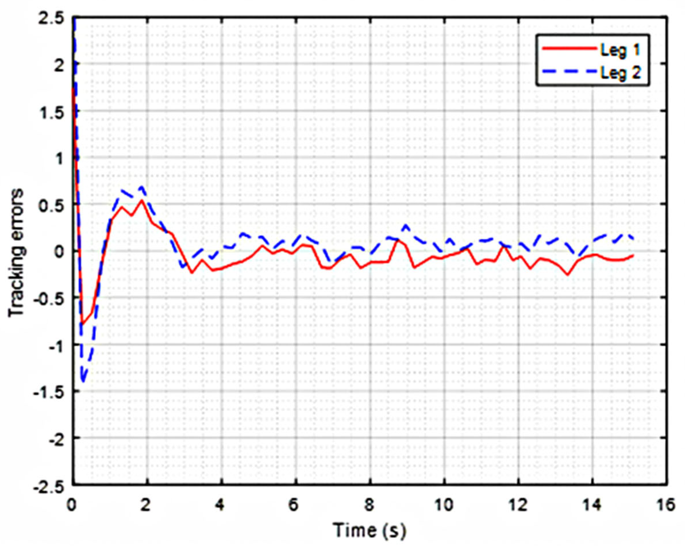
Figure 5 and
Figure 6 illustrate the time trajectories of the tracking errors
(Actuator 1 in solid red line) and
(Actuator 2 in dashed blue line) of the DASCS and SMRACS, respectively. As one can see, the time trajectories of that DASCS’s tracking errors follow each other very closely, while those of the SMRACS do not. For this case, the DASCS has maximum and average synchronization errors of 0.8913 mm and 0.2828 mm, respectively, while the SMRACS has maximum and average synchronization errors of 1.1559 mm and 0.6897 mm, respectively. Studying the transient and steady-state behaviors of the control schemes, we found that the DASCS has better transient and steady-state responses than the SMRACS. In particular, the average tracking errors of the DASCS and the SMRACS for Actuator (leg) 1 are 0.1786 mm and 0.4335 mm, respectively, resulting in the SMRACS’s average tracking errors being 242% of the DASCS’s errors. The average tracking errors of the DASCS and the SMRACS for Actuator (leg) 2 are 0.2231 mm and 1.1233 mm, respectively, resulting in the SMRACS’s average tracking errors being 503% of the DASCS’s errors.
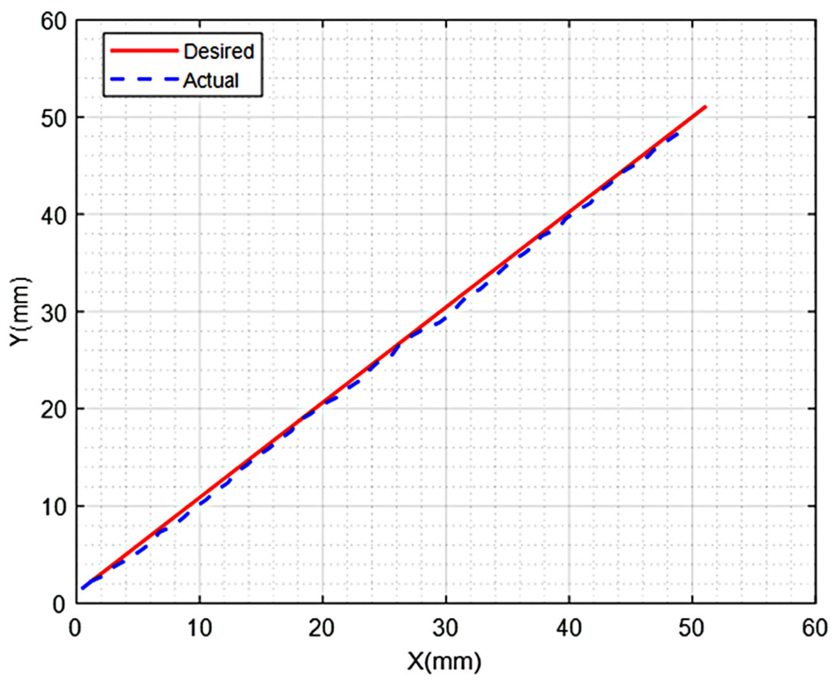
Figure 7 and
Figure 8 show the tracking performance of the DASCS and the SMRACS in the Home Frame, respectively. As one can see, the DASCS provides a better performance in tracking a straight line than the SMRACS.
Table 3 shows that the absolute maximum and average errors of joint and Cartesian variables and the absolute synchronization errors generated in the case of the DASCS are significantly smaller than those of the SMRACS.
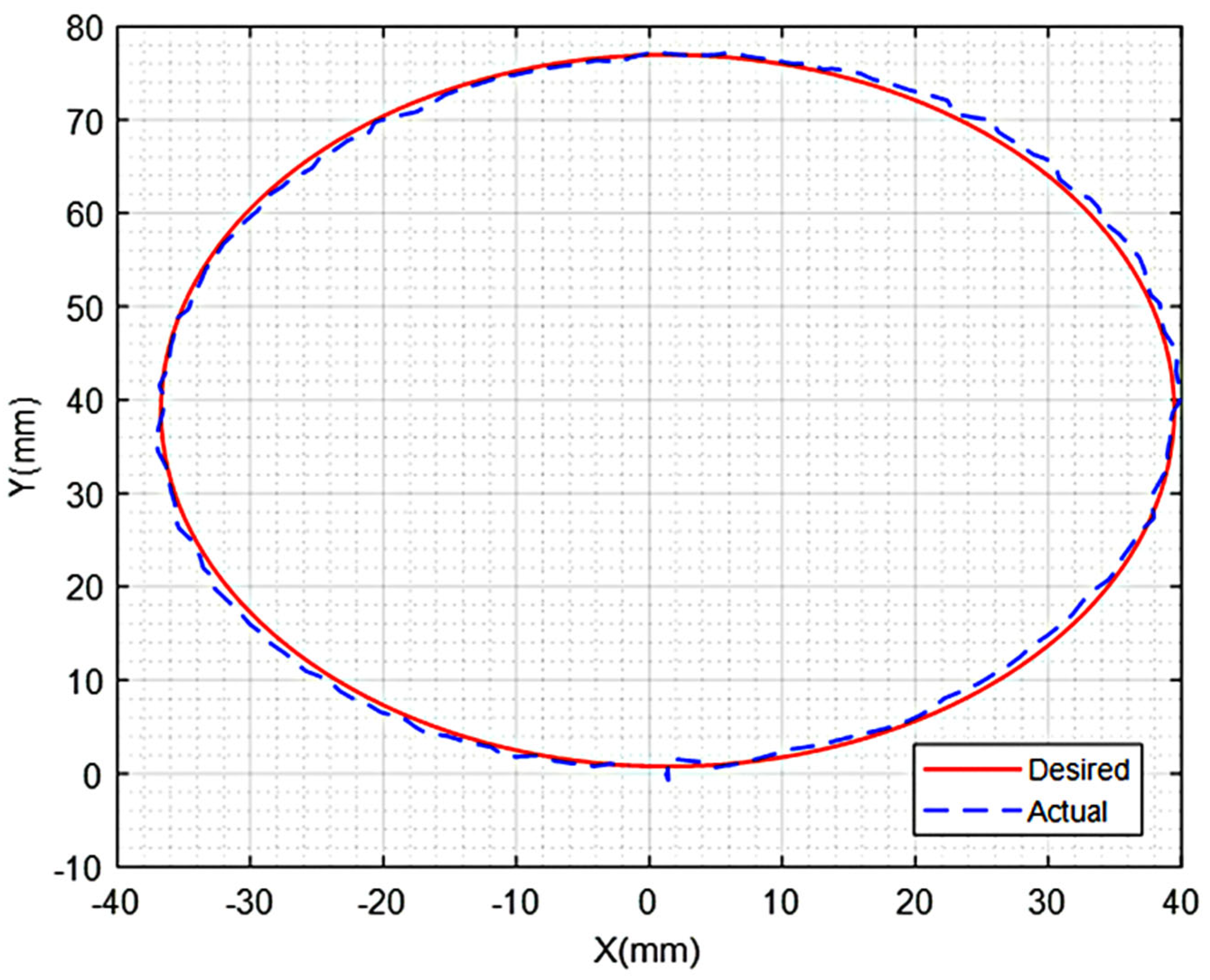
4.2. Experiment 2: Tracking a Circular Motion
In this experiment, the manipulator’s end-effector was controlled by the DASCS and the SMRACS to carry out a circular path with a radius of 38.1 mm with respect to the Home Frame in 45 s. The Trajectory Generator in
Figure 4 first formulated the desired Cartesian motion in terms of
and
and employed the manipulator inverse kinematic Equations (1) and (2) to determine the desired joint variables
and
(t).
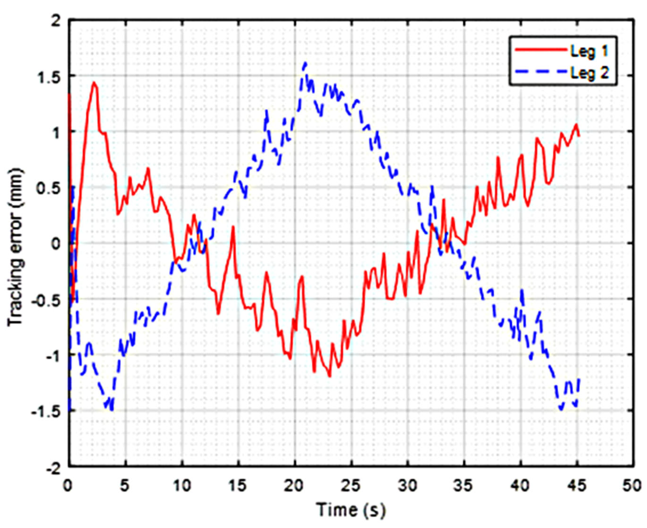
Figure 9 and
Figure 10 illustrate time trajectories of the tracking errors
(Actuator 1 in solid red line) and
(Actuator 2 in dashed blue line) of the DASCS and SMRACS, respectively. As one can see, the time trajectories of the DASCS’s tracking errors follow each other very closely, while those of the SMRACS do not. For this case, the DASCS has maximum and average synchronization errors of 1.1823 mm and 0.3736 mm, respectively, while the SMRACS has maximum and average synchronization errors of 2.8422 mm and 1.2515 mm, respectively. Studying the transient and steady-state behaviors of the control schemes, we found that the DASCS has better transient and steady-state responses than the SMRACS. In particular, the average tracking errors of the DASCS and the SMRACS for Actuator 1 are 0.4536 mm and 0.5228 mm, respectively, resulting in the SMRACS’s average tracking errors being 115% of the DASCS’s errors. The average tracking errors of the DASCS and the SMRACS for Actuator 2 are 0.4497 mm and 0.7461 mm, respectively, resulting in the SMRACS’s average tracking errors being 165% of the DASCS’s errors.
Additionally, the experimental data show that the DASCS has maximum tracking errors of 1.0612 mm and 1.1050 mm, while the maximum tracking errors of the SMRACS are 1.4396 mm and 1.6191 mm, respectively.
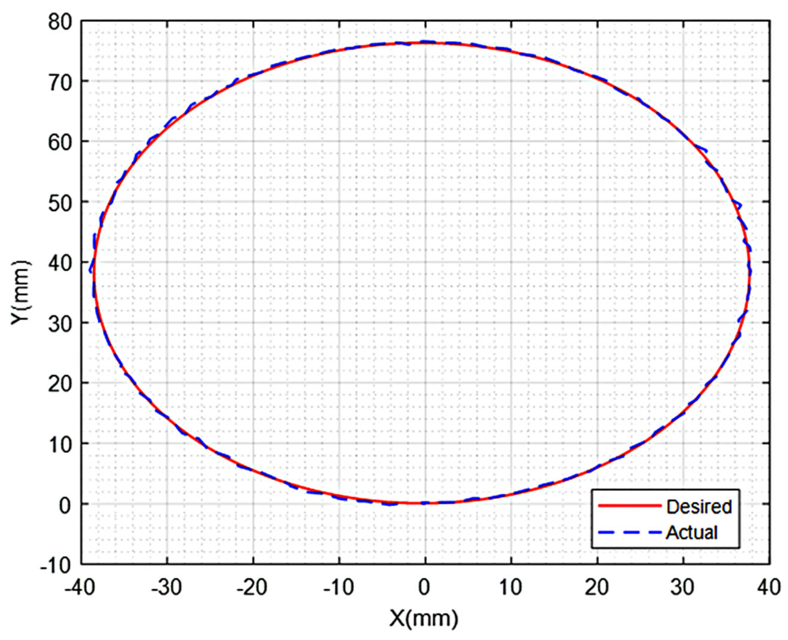
Figure 11 and
Figure 12 show the tracking performance of the two control schemes in the Home Frame. We see that the DASCS provides a better tracking performance than the SMRACS.
Table 4 shows that the absolute maximum and average position and synchronization errors achieved in the case of the DASCS are significantly smaller than those of the SMRACS.
In light of the obtained results of the two performed experiments presented above, it is appropriate to analyze the results and provide resulting findings. We recall that the main difference between the DASCS and SMRACS is that the adaptation law of the DASCS as expressed in Equations (13) and (14) acts on the generalized errors
and
and the cross coupling errors
and
, while the SMRACS acts on the conventional joint errors
and
. Due to the inclusion of the cross coupling error control in the DASCS, we expect it to have better tracking performance than the SMRACS. Quantitatively, according to
Figure 5 for the case of straight-line motion, the synchronized error control of the DASCS enabled it to “synchronize” the time trajectories of joint variable errors
and
, and as a result, they followed each other very closely. On the other hand, without the synchronized error control in the case of the SMRACS, the time trajectories of the joint variable errors were farther apart, as seen in
Figure 6, as compared to those of the DASCS. In addition, a qualitative analysis of the time trajectories of joint variable errors in the case of circular motion based on
Figure 9 and
Figure 10 leads to the same conclusion. Particularly,
Figure 10 shows that time trajectories of the joint variable errors under control of SMARCS were totally out of synchronization. Quantitatively, the results tabulated in
Table 3 and
Table 4 show that the absolute maximum and average errors in Cartesian space (
and
) and joint space (
and
) and the synchronization errors (
and
) of the SMRACS were consistently and significantly higher than those of the DASCS when both control schemes were applied to track the straight-line and circular motions.
5. Conclusions
This paper focused on the experimental evaluation of the performance of a developed DASCS for motion control of CKCM manipulators. In our study, we considered CKCM manipulators because they have several advantages over OKCM manipulators, such as higher stiffness, better positioning accuracy, greater payload, and better stability. Solving control problems for CKCMs would result in higher efficiency and productivity of production processes. To comparatively evaluate the control performance of the developed DASCS, we conducted real-time experiments in which the DASCS and the SMRACS were applied to control a 2-DOF CKCM of a control scheme testbed to track two typical Cartesian motions, namely a straight line and a circular motion. Experimental results confirmed qualitatively and quantitatively that the DASCS had better tracking performance than the SMRACS. We concluded that the main reason causing the SMRACS to perform worse than the DASCS in the motion control of CKCM manipulators was its lack of synchronized error control. To continue the research in this paper, we recommend conducting experimental investigation of the performance of the DASCS on real CKCM manipulators with more DOFs in comparison with other conventional adaptive control schemes. Furthermore, the DASCS should be applied to OCKM robot manipulators, and its performance should be evaluated using computer simulation and experimentation. Additionally, experiments should be conducted to highlight the particular advantages of the DASCS, such as effective management of the interactions between active joints in closed-loop mechanisms, by including tests to simulate such challenges such as intentionally inducing disturbances in a selected joint and then analyzing the robustness of controllers under this circumstance. Finally, future research can be devoted to combining the DASCS with other intelligent control methods, including fuzzy control, neuro fuzzy control, and neural network control, to potentially improve its control performance.

 ,
, 


