Enhancing Supervisory Control with GPenSIM

Abstract

Supervisory control theory (SCT), based on Petri nets, offers a robust framework for modeling and controlling discrete-event systems but faces significant challenges in scalability, expressiveness, and practical implementation. This paper introduces General-purpose Petri Net Simulator and Real-Time Controller (GPenSIM), a MATLAB version 24.1.0.2689473 (R2024a) Update 6-based modular Petri net framework, as a novel solution to these limitations. GPenSIM leverages modular decomposition to mitigate state-space explosion, enabling parallel execution of weakly coupled Petri modules on multi-core systems. Its programmable interfaces (pre-processors and post-processors) extend classical Petri nets’ expressiveness by enforcing nonlinear, temporal, and conditional constraints through custom MATLAB scripts, addressing the rigidity of traditional linear constraints. Furthermore, the integration of GPenSIM with MATLAB facilitates real-time control synthesis, performance optimization, and seamless interaction with external hardware and software, bridging the gap between theoretical models and industrial applications. Empirical studies demonstrate the efficacy of GPenSIM in reconfigurable manufacturing systems, where it reduced downtime by 30%, and in distributed control scenarios, where decentralized modules minimized synchronization delays. Grounded in systems theory principles of interconnectedness, GPenSIM emphasizes dynamic relationships between components, offering a scalable, adaptable, and practical tool for supervisory control. This work highlights the potential of GPenSIM to overcome longstanding limitations in SCT, providing a versatile platform for both academic research and industrial deployment.

1. Introduction

Supervisory control theory in the context of Petri nets is a formal framework for modeling, analyzing, and synthesizing controllers for discrete-event systems [1,2]. In this framework, the uncontrolled system (“plant”) is represented as a Petri net, where places represent system states or conditions, transitions represent events (e.g., actions and tasks), and tokens represent the resources or signals [3,4]. Control specifications for the desired behaviors (such as a maximum of 10 tokens in place p1; buffer control via monitor places [5]) are formalized as linear constraints (e.g., linear inequalities on markings) [6]. A supervisor is synthesized to enforce specifications by either disabling transitions that would violate constraints or monitoring markings (system states) in real time [2]. The approach for the synthesis of supervisors is based on Place Invariants (P-invariants), which enforce linear constraints on markings (e.g., via control places added to the plant Petri net) [6], and maximally permissive control by which all legal behaviors are allowed while illegal ones are prevented [7].

Using Petri nets for supervisory control offers many advantages, such as a graph-based visual front and linear algebraic-based mathematical modeling and analysis on the back end, handling concurrency and resource sharing naturally, and supporting modular supervisor design [3,4,8]. However, it has several limitations, particularly in scalability, expressiveness, and practical implementation (explained in Section 2). Some of these limitations can be overcome with extended Petri nets such as Colored Petri nets (for complex systems with data/variable dependencies) [9] and Timed Petri nets and Stochastic Petri nets (for performance-oriented real-time control) [10]. However, most of the limitations remain unresolved. This paper provides a novel approach based on the General-purpose Petri Net Simulator and Real-Time Controller (GPenSIM) to address these gaps.

The structure of this paper is as follows: Section 2 presents a compact literature review on the limitations of supervisory control based on Petri nets. Section 3 and Section 4 provide formal definitions of Petri nets, as these definitions are expected in works on the modeling of discrete systems. Section 6 introduces GPenSIM, and Section 7 shows how GPenSIM can mitigate some of the limitations of supervisory control. Finally, Section 8 summarizes the findings of this paper.

2. Literature Review

While supervisory control theory based on Petri nets is a powerful framework for discrete-event systems [6,11,12], it has several limitations, particularly in scalability, expressiveness, and practical implementation.

2.1. State-Space Explosion

The computational complexity of synthesizing supervisors grows exponentially with the size of the plant (number of places, transitions, and tokens). This so-called “state-space explosion” is a major problem when Petri nets are used, and also for the synthesis of supervisors [13]. Hence, this problem prevents the applicability of Petri nets for controlling large or complex systems such as industrial automation or multi-agent-based communication systems.

One way to eliminate the state-explosion problem is to modularize the monolithic Petri net model into multiple “Petri Modules,” which can be run on multiple host CPUs. Thus, this modular approach eliminates the state-explosion problem as well as reduces the overall simulation time, as multiple CPUs host these modules [8]. However, the monolithic Petri net model must intrinsically possess laminar flow (no criss-crossing connections) so that it can be decomposed into modules. Additionally, model abstraction has been proposed as a solution [14]. Here, again, abstraction means loss of information; how much information are we willing to sacrifice in order to reduce the number of states? It is a trade-off between depth of information and number of states.

2.2. Scalability in Distributed Systems

Supervisors synthesized by supervisory control theory are meant for centralized control, as there are no measures for distributed control. However, centralized supervisors may not scale well for decentralized or distributed systems due to communication delays and may not work at all in synchronization issues [8]. Hence, Davidrajuh [8] and Yoo and Lafortune [15] propose decentralized or distributed supervisors with localized modular control and minimal coordination between the modules.

2.3. Limited Expressiveness for Nonlinear Constraints

Classical Petri net-based supervisory control relies on linear constraints (e.g., place invariants), and it does not support nonlinear constraints. Additionally, there is no way to enforce temporal, priority-based, or conditional constraints (e.g., “If a fire event occurs, disable the machine for 60 s”). Some temporal constraints can be enforced using Timed/Stochastic Petri nets [10]. Moreover, Basile et al. [7] suggested the use of hybrid methods (such as integrating Petri nets with Automata or logic programming); however, a formal, robust approach does not exist.

2.4. Rigid Enforcement of the Controller

Supervisors synthesized by supervisory control theory often disable all transitions leading to illegal states, which may be too conservative. This excessive conservativeness reduces system flexibility and efficiency, as sometimes the controller blocks legal behaviors unnecessarily. Ghaffari et al. [16] suggested maximally permissive control using the theory of regions as a way to relax the controller’s over-restrictiveness. Yang et al. [17] and Herzig et al. [18] suggested partial observability-aware synthesis to relax the controller.

2.5. Partial Observability Challenges

If some transitions are unobservable, the supervisor cannot always determine the exact system state, and this may lead to incorrect disabling of transitions. Ru and Hadjicostis [19] suggested estimating markings using observers.

2.6. Other Difficulties

There are some other limitations in supervisory control theory based on Petri nets, such as handling unmodeled disturbances. Basile et al. [20] proposed fault-tolerant Petri nets as a remedy and online reconfiguration of supervisors. Moreover, Wang et al. [10] presented the problem of handling real-time and continuous dynamics in supervisors and suggested an approach based on Timed Petri nets. Kaid et al. [21] and Al-Ahmari et al. [22] propose a reconfigurable controller to face dynamic changes in the plant.

2.7. Concluding Remark

The literature review highlights persistent challenges in Petri net-based supervisory control, including state-space explosion, limited expressiveness for nonlinear/temporal constraints, rigid enforcement of controllers, and scalability issues in distributed systems. While extensions like Colored Petri nets and modular approaches offer partial solutions, they often trade off expressiveness, computational efficiency, or practical implementation. These limitations underscore the need for a unified framework that combines modular decomposition, programmable interfaces, and seamless integration with computational tools. GPenSIM addresses these gaps by leveraging the ecosystem of MATLAB to enable scalable, expressive, and adaptable supervisory control, as detailed in the subsequent sections.

3. Petri Nets

Petri nets have gone through many versions (extensions and subclasses), mainly to incorporate time and to increase their modeling power [4]. In this section, we provide the formal definitions. For a thorough study on Petri nets, the following textbooks are suggested [23,24,25,26,27].

3.1. Definition: P/T Petri Nets

The Place-Transition Petri net (P/T Petri net, for short) is defined as a four-tuple [4,28,29]:

$$PTN=(P,T,A,M_0),$$

where the following applies:

• P is a finite set of places, $P=\{p_1,p_2,\dots ,p_{n_p}\}.$
• T is a finite set of transitions, $T=\{t_1,t_2,\dots ,t_{n_t}\}$.   P ∩ T = ∅.
• A is the set of arcs (from places to transitions and from transitions to places). $A\subseteq (P\times T)\cup (T\times P).$ The default arc weight W of $a_{ij}$ ($a_{ij}\in A$, an arc going from $p_i$ to $t_j$ or from $t_i$ to $p_j)$ is one, unless noted otherwise.
• M is the row vector of markings (tokens) on the set of places.
  $M=[M\left(p_1\right),M\left(p_2\right),\dots ,M\left(p_{n_p}\right)]\in N^{n_p}$,    $M_0$ is the initial marking. Due to the markings, a $PTN=(P,T,A,M)$ is also called a marked P/T Petri net.

P/T Petri nets do not involve time. Hence, P/T Petri nets are insufficient to model engineering systems, as time is one of the key performance indicators (KPI). Hence, a Timed Petri net is an extended Petri net incorporating time.

3.2. Definition: Timed Petri Net

The Timed Petri net (TPN, for short) is defined as a five-tuple [30,31]:

$$TPN=(P,T,A,M,FT),$$

where the following applies:

• $(P,T,A,M)$ is a Marked Petri net;
• $FT$ is a mapping of T into ${\mathbb{R}}^{+}$:
  $\forall t\in T,FT\left(t\right)\in {\mathbb{R}}^{+},FT\left(t\right)>0$.

$FT\left(t\right)$ is known as the firing times of the transitions and is defined to be greater than zero.

4. Modular Petri Nets

The literature review reveals many definitions of Modular Petri nets [32,33,34,35,36,37,37]. Davidrajuh [8,38] proposed a new type of Modular Petri net, which is implemented in the software GPenSIM version 11 (2025).

4.1. Modular Petri Net and Petri Modules

A modular Petri net is composed of one or more Petri modules and zero or more Inter-Modular connectors (IMCs).

$$\mathbf{Modular}\mathbf{Petri}\mathbf{Net} \left(\mathbf{MPN}\right)=\mathbf{Petri}\mathbf{Modules}+\mathbf{IMCs} (\mathbf{Inter}-\mathbf{Modular}\mathbf{Connectors})$$

4.2. Formal Definition of MPN

An MPN is defined as a two-tuple:

$$MPN=(\mathbb{M},\mathcal{C})$$

• $\mathbb{M}={\sum }_{i=0}^m{\mathrm{\Phi }}_i$ (one or more Petri Modules);
• $\mathcal{C}={\sum }_{j=0}^n{\mathrm{\Psi }}_j$ (zero or more IMCs).

4.3. Formal Definition of Petri Module

A Petri Module is defined as a six-tuple:

$$\mathrm{\Phi }=(P_{L\mathrm{\Phi }},T_{IP\mathrm{\Phi }},T_{L\mathrm{\Phi }},T_{OP\mathrm{\Phi }},A_{\mathrm{\Phi }},M_{\mathrm{\Phi }0}),$$

where the following applies:

• $T_{IP\mathrm{\Phi }}\subseteq T$: $T_{IP\mathrm{\Phi }}$ (Input Ports);
• $T_{L\mathrm{\Phi }}\subseteq T$: $T_{L\mathrm{\Phi }}$ (local transitions);
• $T_{OP\mathrm{\Phi }}\subseteq T$: $T_{OP\mathrm{\Phi }}$ (Output Ports);
• $T_{IP\mathrm{\Phi }}$, $T_{L\mathrm{\Phi }}$, and $T_{OP\mathrm{\Phi }}$ are all mutually exclusive:
  $T_{IP\mathrm{\Phi }}\cap T_{L\mathrm{\Phi }}=T_{L\mathrm{\Phi }}\cap T_{OP\mathrm{\Phi }}=T_{OP\mathrm{\Phi }}\cap T_{IP\mathrm{\Phi }}=\mathrm{\varnothing }$.
• $T_{\mathrm{\Phi }}=T_{IP\mathrm{\Phi }}\cup T_{L\mathrm{\Phi }}\cup T_{OP\mathrm{\Phi }}$ (the transitions of the module);
• $P_{L\mathrm{\Phi }}\subseteq P$: The local places, as a module has only local places, $P_{\mathrm{\Phi }}\equiv P_{L\mathrm{\Phi }}$;
• $\forall p\in P_{L\mathrm{\Phi }}$:

  –

  $•p\in (T_{\mathrm{\Phi }}\cup \mathrm{\varnothing })$ (a local place can be input by transition inside the module or none);

  –

  $p•\in (T_{\mathrm{\Phi }}\cup \mathrm{\varnothing })$ (an output of a local place can be transition inside the module or none);

• $\forall t\in T_{L\mathrm{\Phi }}$:

  –

  $•t\in (P_{L\mathrm{\Phi }}\cup \mathrm{\varnothing })$ (input place of a module transition is a local place or none);

  –

  $t•\in (P_{L\mathrm{\Phi }}\cup \mathrm{\varnothing })$ (output place of a module transition is a local place or none);

• $\forall t\in T_{IP\mathrm{\Phi }}$:

  –

  $•t\in (P_{L\mathrm{\Phi }}\cup P_{IM}\cup \mathrm{\varnothing })$ (input places of Input Ports can be local places or places in IMCs or none);

  –

  $t•\in (P_{L\mathrm{\Phi }}\cup \mathrm{\varnothing })$ (output places of Output Ports can be local places or places in IMCs or none);

• $\forall t\in T_{OP\mathrm{\Phi }}$:

  –

  $•t\in (P_{L\mathrm{\Phi }}\cup \mathrm{\varnothing })$ (input places of Output Ports can be local places or an empty set);

  –

  $t•\in (P_{L\mathrm{\Phi }}\cup P_{IM}\cup \mathrm{\varnothing })$ (output places of Output Ports can be local places, IM places, or none);

• $A_{\mathrm{\Phi }}\subseteq (P_L\times T_{\mathrm{\Phi }})\cup (T_{\mathrm{\Phi }}\times P_L)$, where $a_{ij}\in A_{\mathrm{\Phi }}$ (internal arcs);
• $M_{\mathrm{\Phi }0}=\left[M\left(p_L\right)\right]$ (initial markings in local places).

4.4. Formal Definition of Inter-Modular Connector

An Inter-modular Connector (IMC) is defined as a four-tuple:

$$\mathrm{\Psi }=(P_{\mathrm{\Psi }},T_{\mathrm{\Psi }},A_{\mathrm{\Psi }},M_{\mathrm{\Psi }0})$$

where the following applies:

• $P_{\mathrm{\Psi }}\subseteq P$: $P_{\mathrm{\Psi }}$ is the set of places in the IMC (known as the IM places) $\forall p\in P_{\mathrm{\Psi }}$;

  –

  $•p\in (T_{OP}\cup T_{\mathrm{\Psi }}\cup \mathrm{\varnothing })$ (input transitions of IM places can be Output Ports of modules, IM transitions of this specific IMC, or none);

  –

  $p•\in (T_{IP}\cup T_{\mathrm{\Psi }}\cup \mathrm{\varnothing })$ (output transitions of IM places can be Input Ports of modules, IM transitions of this specific IMC, or none)

  (IM places are not allowed to have direct connections with local transitions of modules);

• $\forall p\in P_{\mathrm{\Psi }},\forall ip\notin P_{{\mathrm{\Phi }}_i}$ (a local place of a module can not be an IM place);
• $T_{\mathrm{\Psi }}\subseteq T$: $T_{\mathrm{\Psi }}$ is the transitions of the IMC (aka IM transitions) $\forall t\in T_{\mathrm{\Phi }}$;

  –

  $•t\in (P_{\mathrm{\Psi }}\cup \mathrm{\varnothing })$ (input places of IM transitions can be IM places of this specific IMC or none);

  –

  $t•\in (P_{\mathrm{\Psi }}\cup \mathrm{\varnothing })$ (output places of IM transitions can be IM places of this specific IMC or none).

• $\forall t\in T_{\mathrm{\Psi }},\forall it\notin T_{{\mathrm{\Phi }}_i}$ (an IM transition is not allowed to be a member of any modules);
• $A_{\mathrm{\Psi }}\subseteq (P_{\mathrm{\Psi }}\times (T_{\mathrm{\Psi }}\cup T_{IP}))\cup ((T_{\mathrm{\Psi }}\cup T_{OP})\times P_{\mathrm{\Psi }})$, where $a_{ij}\in A_{\mathrm{\Psi }}$ is the IMC arc;
• $M_{\mathrm{\Psi }0}=\left[M\left(p_{\mathrm{\Psi }}\right)\right]$ initial markings in IM places.

4.5. Real-World Applications of Modular Petri Nets

While this section focuses on the theoretical framework of Modular Petri nets (MPNs), real-world applications are essential to demonstrate their practical utility. For comprehensive case studies—including examples drawn from an automotive manufacturing plant in Poland—readers are directed to Davidrajuh (2021) [8]. The examples presented in [8] showcase MPNs in industrial-scale scenarios, validating the scalability and adaptability of the proposed modular approach.

5. Comparison Between the Modular Petri Nets of GPenSIM and Other Modular Petri Nets

This section presents a detailed comparison between the Modular Petri nets (MPNs) of GPenSIM and other Modular Petri net approaches. The comparison focuses on key aspects such as modularity, expressiveness, scalability, and practical implementation.

5.1. Modularity and Composition

In summary, in the MPN [8] of GPenSIM, the following applies:

• A Petri Module is defined as a six-tuple $(P_{L\mathrm{\Phi }},T_{IP\mathrm{\Phi }},T_{L\mathrm{\Phi }},T_{OP\mathrm{\Phi }},A_{\mathrm{\Phi }},M_{\mathrm{\Phi }0})$, with explicit Input/Output Ports ($T_{IP\mathrm{\Phi }},T_{OP\mathrm{\Phi }}$) and local transitions ($T_{L\mathrm{\Phi }}$);
• Uses Inter-Modular Connectors (IMCs) to link modules, ensuring no direct connections between local transitions of different modules;
• Supports hierarchical abstraction and parallel execution on multi-core systems.

Other MPN Approaches:

Kindler and Petrucci (2009) [32] formalized modularity via “module nets” with export/import interfaces, but this lacks explicit port definitions. Lakos and Petrucci (2010) [37] focused on state-space reduction via prioritization but did not address distributed execution.

5.2. Expressiveness and Constraints

The MPN of GPenSIM enhances expressiveness via programmable pre/post-processors (MATLAB scripts) to enforce nonlinear, temporal, and conditional constraints (e.g., “disable if $p2>10$ for 60 min”). The programmable pre/post-processors also support dynamic adaptation (e.g., relaxing constraints based on real-time state) [39].

Other MPN Approaches:

Colored Petri nets [9] use data types (colors) for complex dependencies but lack programmable interfaces. Wang and Wang (2007) [36] present object-oriented modularity for service-oriented applications but no support for real-time constraints.

5.3. Scalability and State-Space Explosion

The MPN of GPenSIM mitigates state-space explosion by decomposing monolithic nets into weakly coupled modules (laminar-flow systems) and by moving control logic to processors (no additional states), which enables distributed control with minimal coordination [8]. More explanation is given in Section 7.

Other MPN Approaches:

Righini (1993) [33] modularized production systems but assumed centralized execution. Latorre-Biel et al. (2017) [35] focused on compactness but lacked parallel execution support.

5.4. Practical Implementation

The MPN of GPenSIM is integrated with MATLAB for real-time control, hardware/software interfacing, and data analysis. Case studies show 30% downtime reduction in manufacturing [21].

Other MPN Approaches:

Lee et al. (1998) [34] integrated use-case analysis but with no real-time control features.

5.5. Summary

Table 1. Summary table: The MPN of GPenSIM vs. other MPNs.

Feature	GPenSIM MPN	Other MPN Approaches
Modularity	Explicit ports, IMCs	Interface-based (e.g., export/import)
Expressiveness	Programmable (MATLAB), nonlinear/temporal constraints	Limited to linear/data types (e.g., Colored PN)
Scalability	Parallel execution, state-space reduction	Centralized, compact state spaces
Implementation	MATLAB integration, real-time control	Theoretical or limited to simulation

summarizes the findings.

In summary, the key advantages of the MPN of GPenSIM are the following:

1.

Theory of connection: Embodies dynamic interdependencies (Bertalanffy; Forrester); see Section 6.1;

2.

Industrial applicability: Bridges theory/practice via MATLAB (e.g., [21]);

3.

Flexibility: Customizable processors vs. rigid formalisms in other MPNs.

The limitations of the MPN of GPenSIM are the following:

• Requires laminar-flow models for decomposition;
• Lacks native formal verification (though bridges to NuSMV exist).

In conclusion, the MPN of GPenSIM stands out for its practicality, expressiveness, and scalability, addressing gaps in classical MPNs (e.g., rigid constraints and centralized execution).

6. GPenSIM: A Modular Petri Net Framework for Scalable Supervisory Control

GPenSIM is a MATLAB-based Petri net tool developed by the first author of this paper. A C++ programming language-based prototype of GPenSIM was initially developed, called PenSIM (Petri Net Simulator). However, the prototype faced significant limitations in managing interdependencies—both among the Petri net elements and with external systems. To address these challenges, GPenSIM was redeveloped as a MATLAB toolbox, offering improved functionality and flexibility.

GPenSIM stands out from other Petri net tools due to its flexibility, integration with MATLAB, and focus on customization [40,41]. GPenSIM provides an interface—the pre-processors and post-processors—that gives a distinctive programming approach to make Petri net models flexible, as explained in the following subsections.

6.1. “The Theory of Connection”-Based Design

GPenSIM was designed based on the theory of connection. The theory of connection is a concept that appears in different fields (e.g., psychology, sociology, network theory, etc.) with varying interpretations. However, in the context of systems theory, the theory of connection (a.k.a. the principle of interconnectedness) refers to the fundamental idea that elements of a system are interdependent, and their relationships determine the system’s behavior.

According to the theory of connection in systems theory, systems are not merely collections of parts but networks of dynamic relationships. The connections (flows, feedback loops, and dependencies) between elements are as critical as the elements themselves. The concept is interdependence—no element operates in isolation, as changes in one element ripple through the system. Moreover, the connections (loops) create reinforcing, balancing, or stabilizing effects. Additionally, the theory of connection emphasizes Network Structure, meaning the pattern of connections (centralized, decentralized, and modular) determines adaptability, and that systems are defined by their connections to/from the environment (their boundaries and openness).

The theoretical foundations for the theory of connection were laid by Ludwig von Bertalanffy [42,43], Jay Forrester [44,45], and Fritjof Capra [46,47]. However, GPenSIM was designed following the guidelines provided by the legendary Norwegian professor Øyvind Bjørke in his book on “Manufacturing Systems Theory” [48], and in some follow-up works [49].

6.2. GPenSIM Processors

Since GPenSIM runs on the MATLAB platform, it allows for the seamless use of the computational power of MATLAB (matrix operations, advanced statistics, control systems, and AI/ML/DL toolboxes) to be integrated with Petri nets [39,40]. Since MATLAB provides hundreds of functions in virtually any branch of engineering, making Petri net models adapted to different domains becomes easy. Moreover, after Petri net simulations, modelers can leverage the plotting and data analysis tools of MATLAB for results.

At a minimum, implementing a Petri net model with GPenSIM involves four M-files [39,50]:

1.

Petri net definition file (PDF): This file defines the static Petri net graph (places, transitions, and arcs). This file will be executed only once to create a MATLAB structure representing the topological information of this file.

2.

The main simulation file (MSF): This file declares the initial dynamics (e.g., initial tokens and firing times of transitions) and starts the simulations. Once the simulation is started, the GPenSIM compiler takes over to run the simulation. When the simulations are complete, control is passed back to this file so that the simulation results can be analyzed and plotted.

3.

Pre-processors: Whenever transitions are enabled, pre-processors are executed. Only if the corresponding pre-processors return a logical one will the transition be allowed to start firing.

4.

Post-processors: Whenever transitions complete firing, post-processors are executed.

This means that whenever a transition starts firing and completes firing, there will be a processor file executed by the compiler. Hence, it is the processor files (pre-processors and post-processors) that work as the interface, both intra-model (connecting the elements of the model) and between the model and the external world.

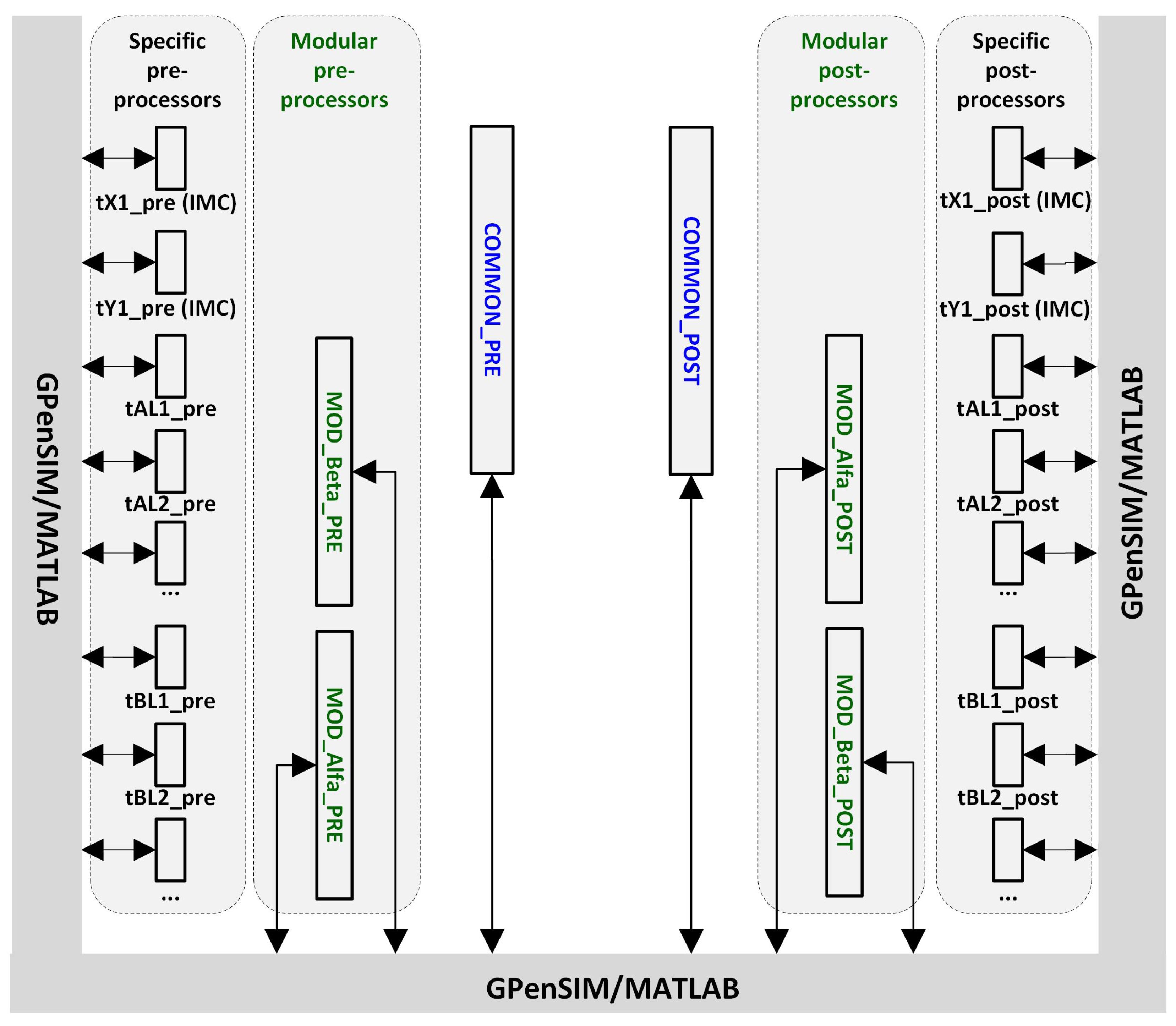
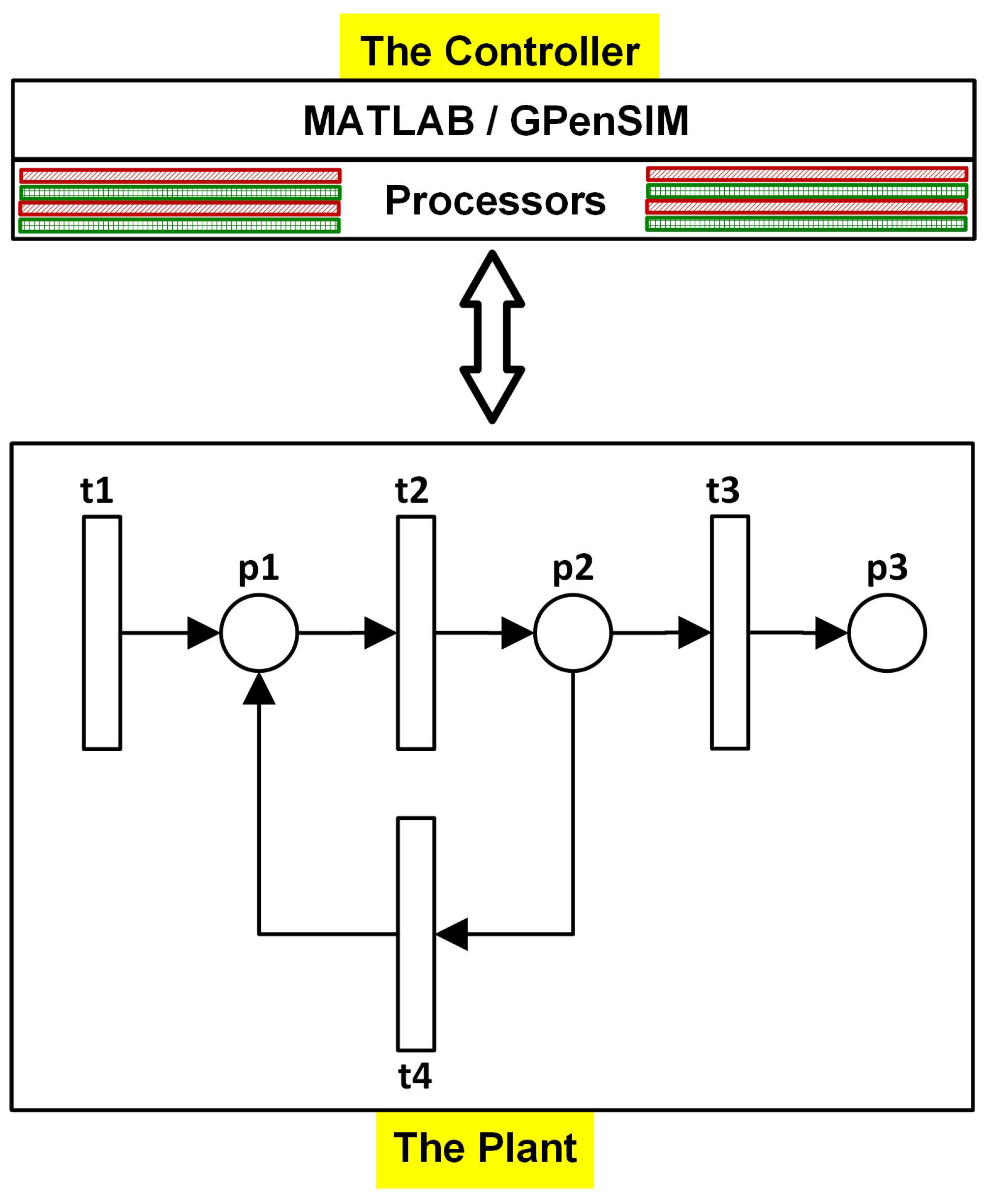
6.3. Integration with MATLAB and the External World

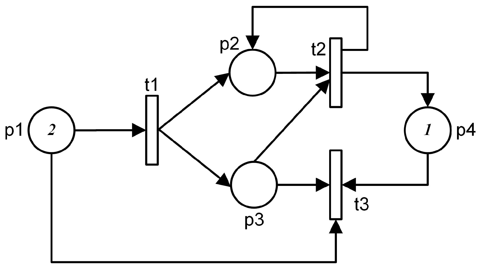
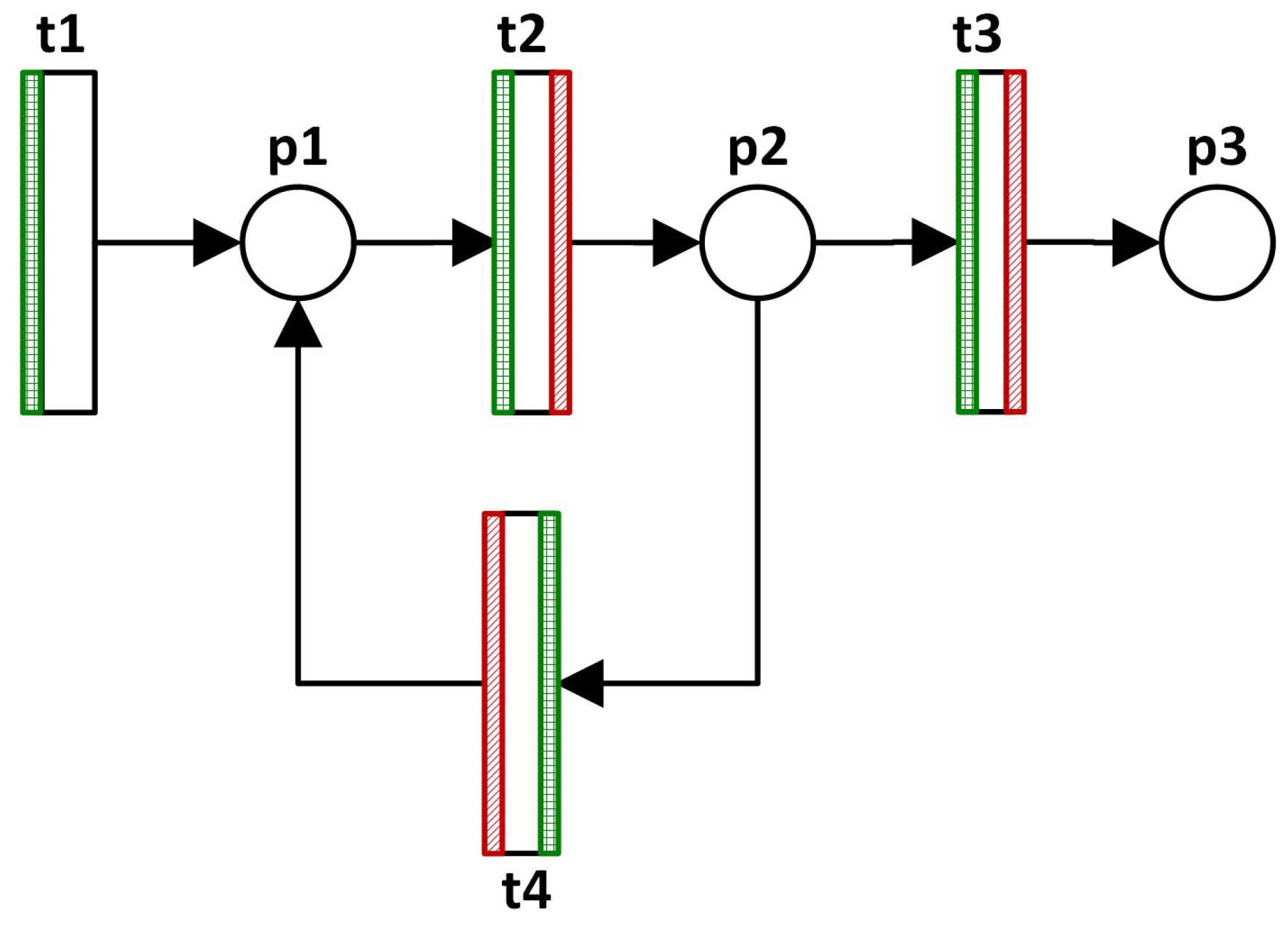
Figure 1 shows a small monolithic (non-modular) Petri net, consisting of four places (p1 to p4) and three transitions (t1 to t3). In GPenSIM, the interface for monolithic Petri net models is different from that of modular Petri nets. For a monolithic Petri net, there are two groups of processors: specific processors and common processors. For example, whenever t1 is enabled, its specific pre-processor t1_pre will be executed if it exists. Additionally, the common pre-processor COMMON_PRE will be executed if it exists, too. 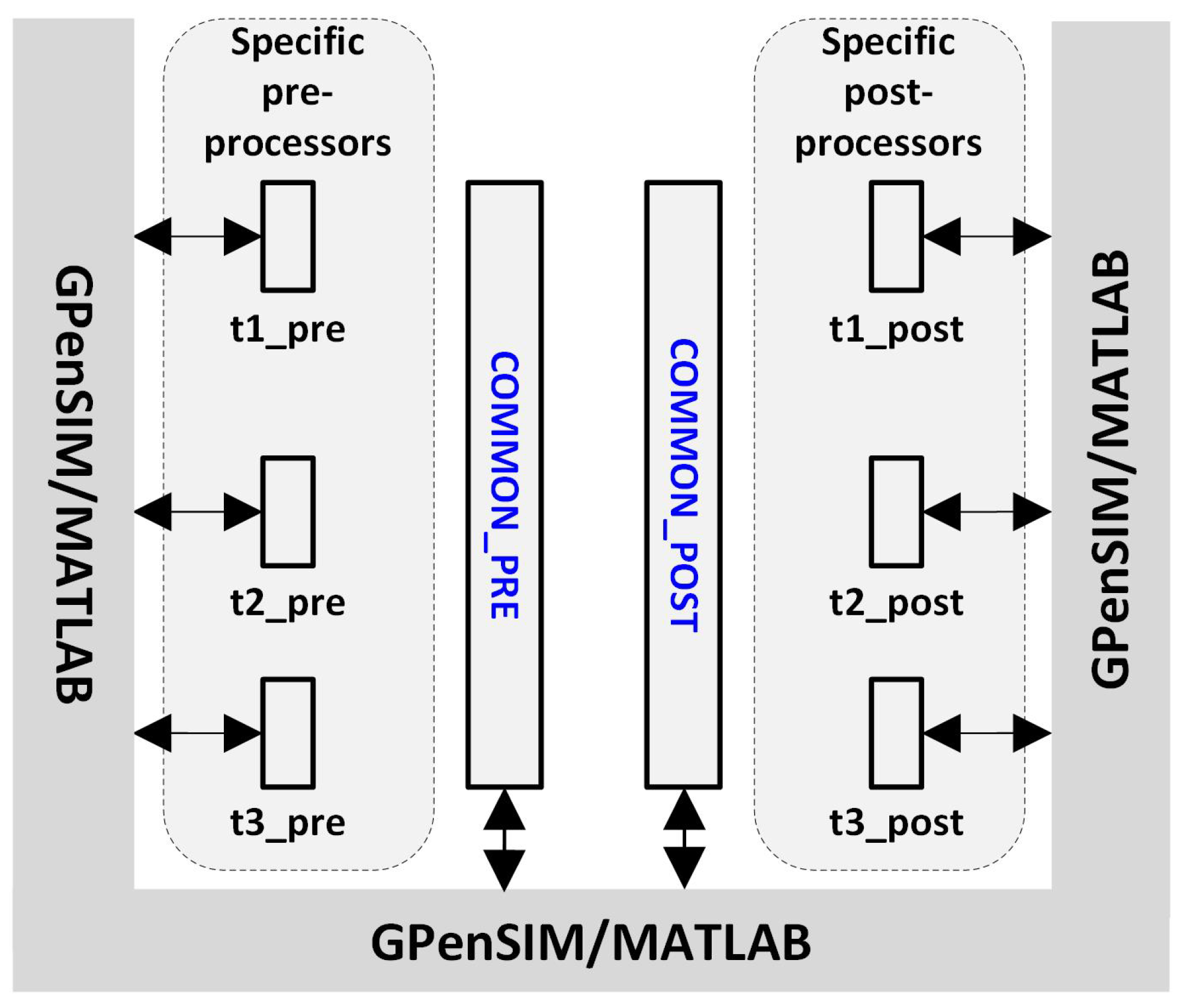Figure 2 shows the processors for the monolithic Petri net shown in Figure 1.

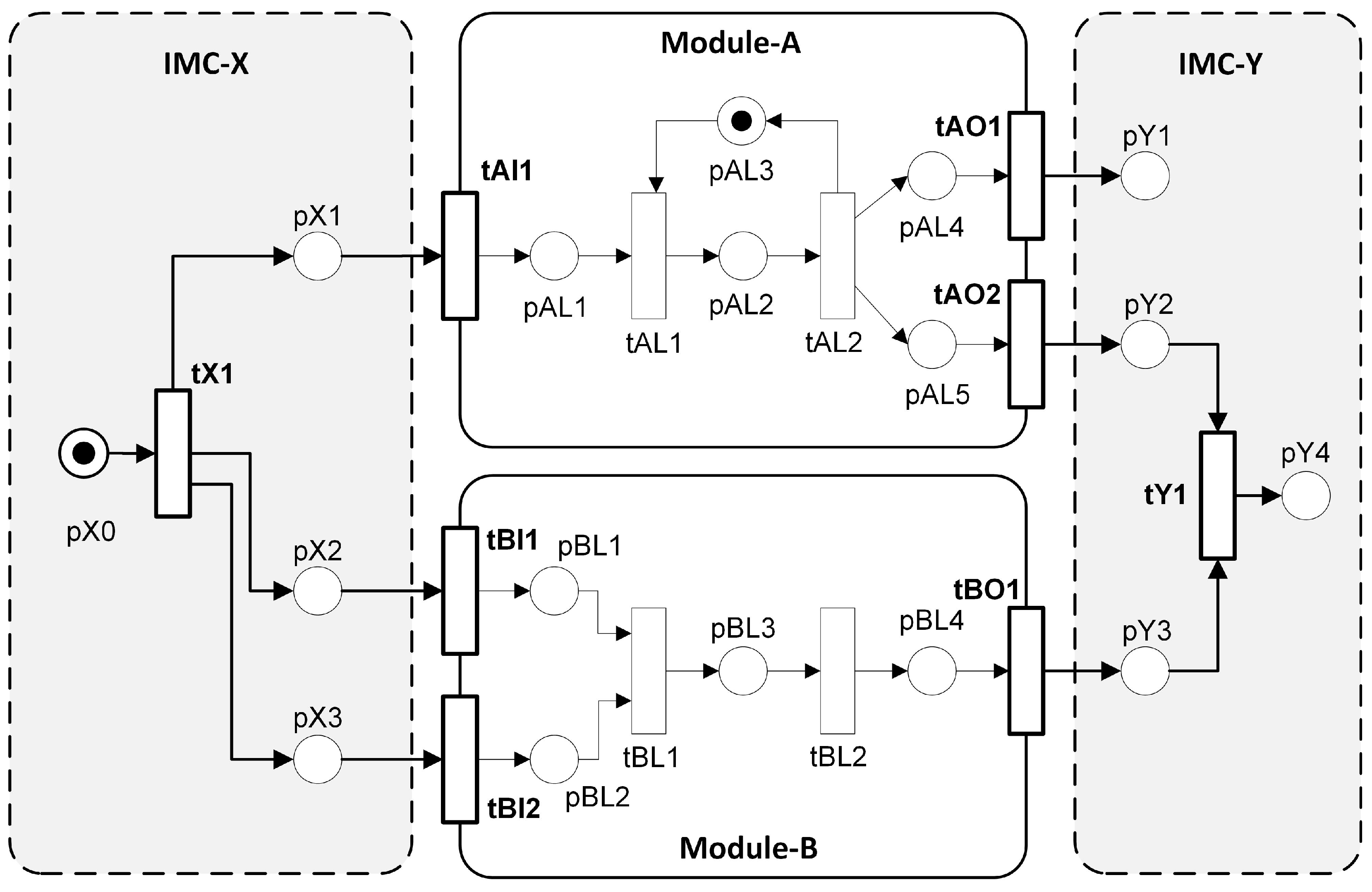
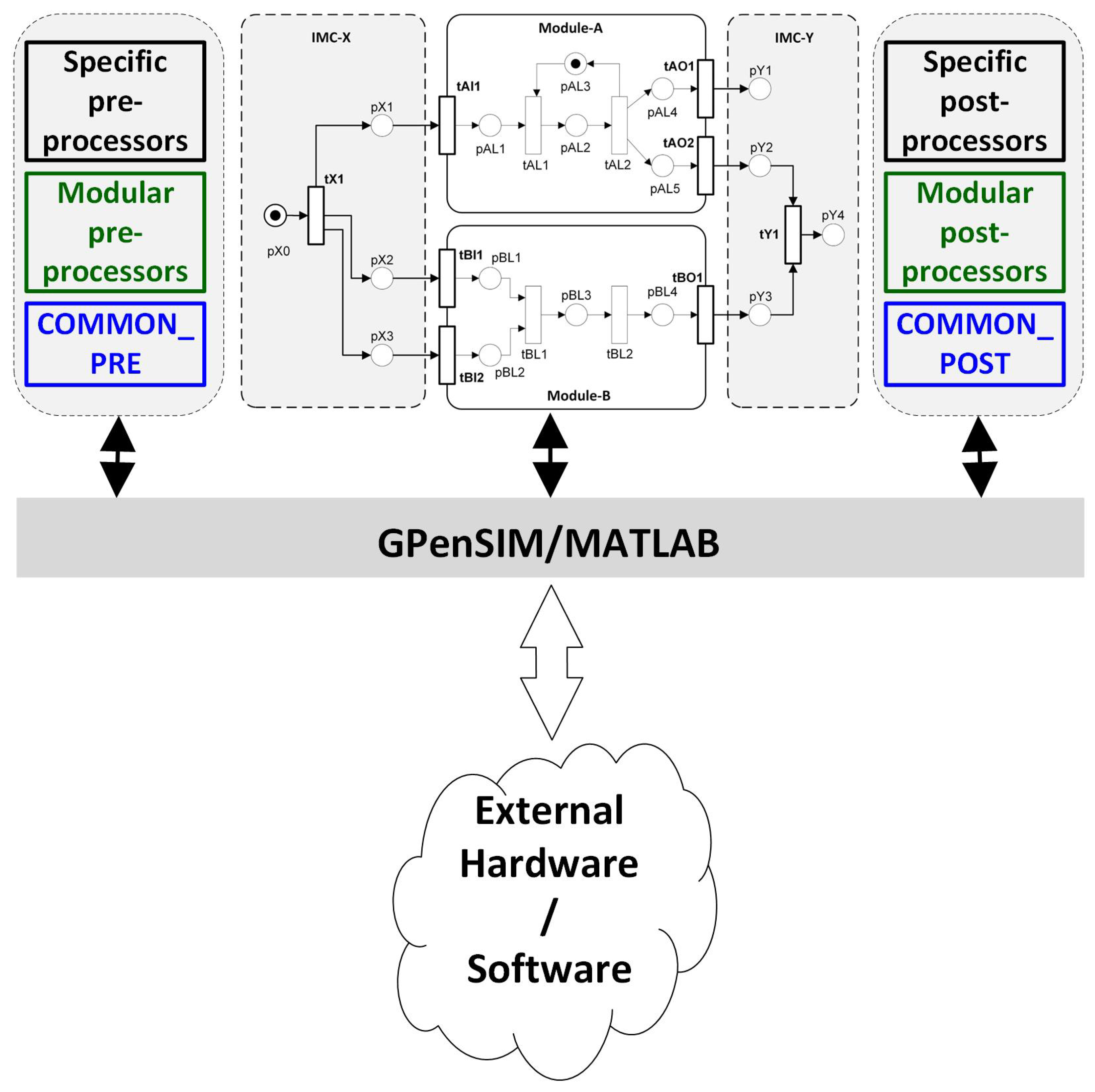
Figure 3 shows a small modular Petri net, consisting of two “Petri Modules,” Module-Alfa and Module-Beta, and two “Inter-Modular Connectors,” IMC-X and IMC-Y. For modular Petri nets, there are three groups of processors; in addition to specific processors and common processors, there are also modular processors. For example, for the modular Petri net shown in Figure 3, whenever tAI1 (an Input Port), tAO1 (an Output Port), or tAL1 (a local transition) is enabled, its modular pre-processor MOD_Alfa_PRE will be executed if it exists. Figure 4 shows the processors for the modular Petri net shown in Figure 3.

In addition to functioning as a Petri net simulator, GPenSIM is also designed to function as a real-time controller. A literature study reveals that some works have used GPenSIM as a controller [21,40]. Figure 5 shows the use of processors as the interface when Petri net models are used to interact with and control external software and hardware.

7. Discussion: Enhancing Supervisory Control with GPenSIM

GPenSIM is grounded in the systems theory principle of interconnectedness, which posits that system behavior emerges from dynamic relationships between components rather than from isolated elements. This principle, rooted in the works of Bertalanffy [42], Forrester [51], and Capra [46], emphasizes the following:

• Interdependence: Transitions, places, and tokens interact via feedback loops and dependencies, mirroring real-world discrete-event systems.
• Network structure: Modular design patterns (centralized vs. decentralized) determine adaptability, aligning with supervisory control challenges in distributed systems (Section 2.2).
• Boundary dynamics: The GPenSIM interface, e.g., the processors (pre/post-processors), models interactions between the Petri net and its environment, addressing partial observability (Section 2.5) and unmodeled disturbances (Section 2.6).

In the following subsection, we shall see how GPenSIM can help solve some of the difficulties we face in supervisory control theory.

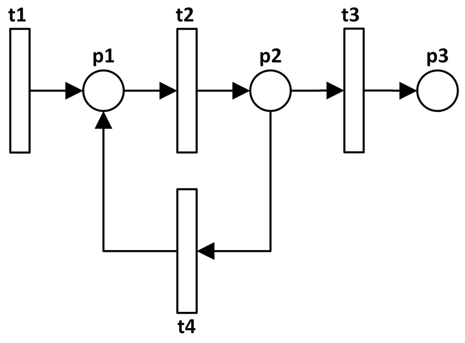
7.1. Reducing State-Space Explosion: Moving Control Logic from Controller to Processors

GPenSIM offers a unique solution to mitigate the state-space explosion problem. As we know, the number of states increases exponentially with the number of places, transitions, and tokens. Hence, embedding a supervisor (a controller with multiple control places and their tokens) on top of a plant to create a controlled system will dramatically increase the total number of states. To address this, GPenSIM provides a unique solution: mapping the controller logic into processors so that the controlled system consists of the plant and the processors without additional state overhead.

For example, Figure 6 shows a simple plant with three places, four transitions, and no initial tokens. Consider the following three constraints:

1.

The number of tokens in p1 must always be less than or equal to 10;

2.

The number of tokens in p2 must always be less than or equal to 5;

3.

The difference between the tokens in p1 and p2 must always be less than or equal to 2.

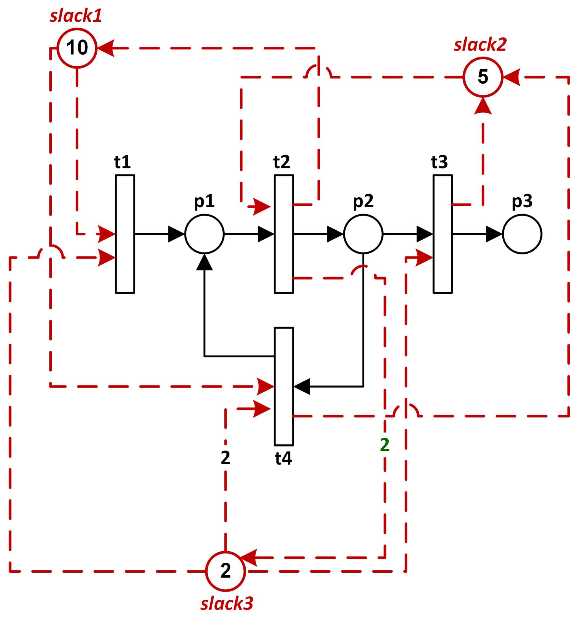
Figure 7 shows the controlled system synthesized using supervisory control theory, assuming all transitions are observable and controllable. The resulting supervisor includes three control places and a total of 17 tokens, which will inevitably cause the state-space of the controlled system to explode.

The built-in function of GPenSIM control2processors maps the supervisor into program code, automatically generating pre-processors and post-processors. This moves the supervisor out of the controlled system, leaving the controlled system as the original Petri net representing the plant. Figure 8 shows the controlled system with processors.

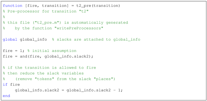
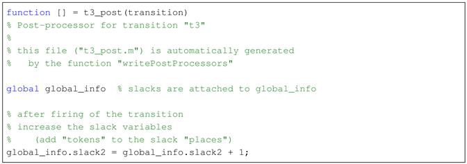
Listing 1 shows one of the pre-processors, t2_pre, automatically generated by the control2processors function of GPenSIM. Listing 2 shows one of the post-processors, t3_post.

Listing 1. Specific pre-processor “t2_pre”

Listing 2. Specific post-processor “t3_post”

In addition to avoiding state-space explosion, the GPenSIM approach of moving the supervisor’s control logic into processor files offers another advantage. As shown in Figure 9, the controlled system can be implemented in real life as a real-time controller for a physical (real-world) plant. Thus, GPenSIM provides a practical solution for developing industrial supervisory controllers.

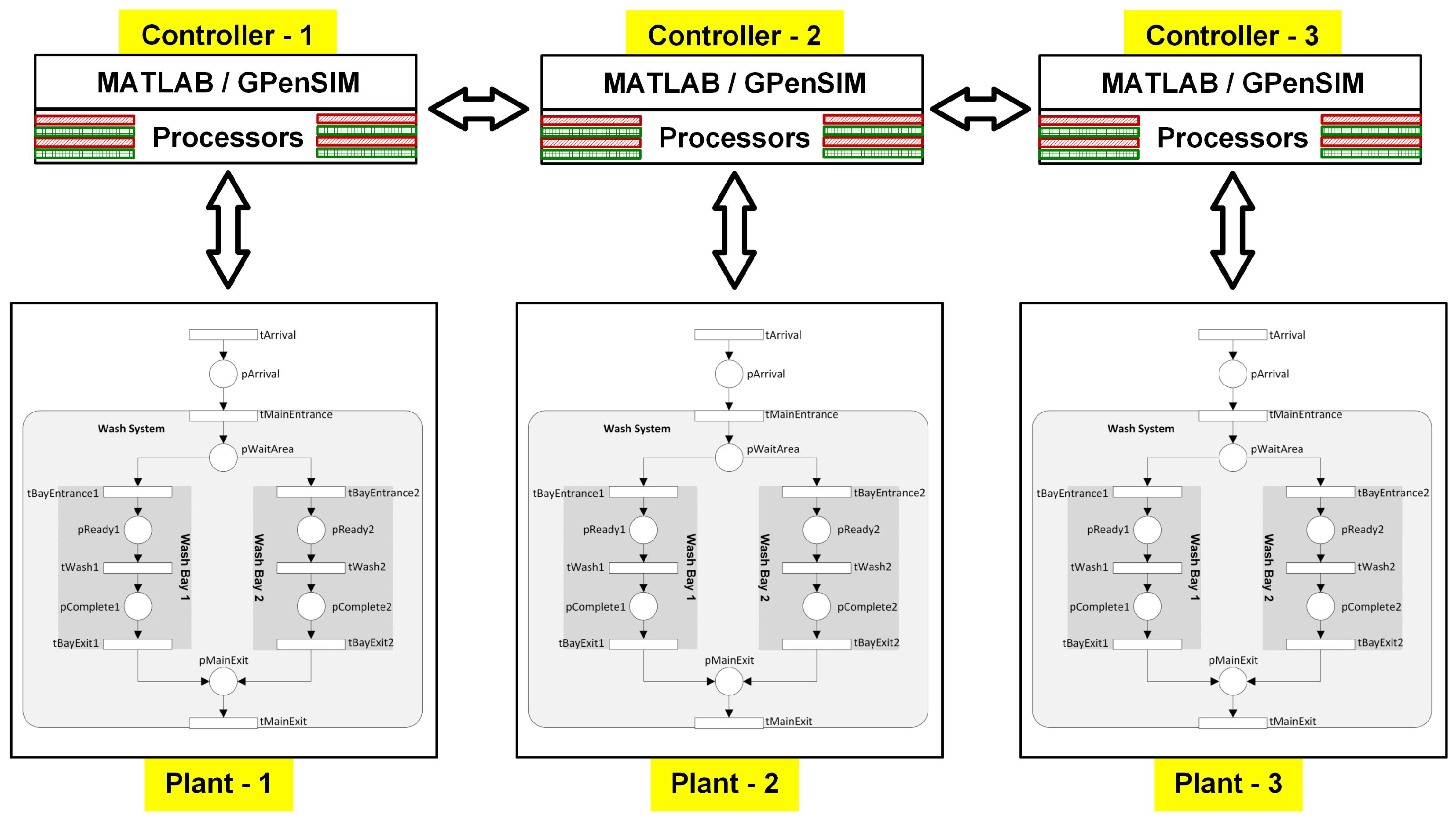
7.2. Increasing Scalability in Distributed Systems

GPenSIM supports modular Petri nets, as defined in [8]. This enables the development of multiple supervisors, each controlling a decentralized plant. These supervisors are implemented as “Petri Modules” that communicate over a shared bus. While operating independently, the distributed supervisors can also collaborate to make global decisions, requiring only minimal coordination between them. Figure 10 illustrates this architecture, showing a set of supervisors managing a decentralized plant.

The modular architecture of GPenSIM directly tackles the state-space explosion problem (Section 2.1) via the following:

• Decomposition: Partitioning monolithic Petri nets into weakly coupled Petri Modules (Figure 3), enabling parallel execution on multi-core systems. This reduces computational complexity from $O\left(n^k\right)$ to $O\left(n\right)$ for laminar-flow systems [8].
• Hierarchical Abstraction: Modules can operate at varying granularity levels, trading off detail for scalability—a key consideration in industrial automation [14].

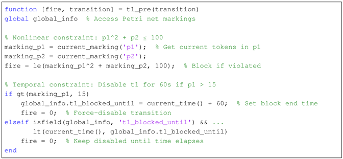
7.3. Enhanced Expressiveness via Programmable Interfaces

Classical Petri nets lack support for nonlinear or temporal constraints (Section 2.3). GPenSIM addresses this through programmable processors, enabling the following:

• Nonlinear constraints (e.g., quadratic, exponential) via MATLAB expressions;
• Temporal/conditional logic (e.g., disabling transitions dynamically).

• Example: Enforcing Nonlinear and Temporal Constraints

Consider a plant with places p1 and p2. We enforce the following:

1.

Quadratic constraint: ($\mathbf{p}{\mathbf{1}}^2+\mathbf{p}\mathbf{2}\le 100$);

2.

Temporal constraint: Transition t1 is disabled for 60 s if p1 exceeds a threshold.

GPenSIM Implementation (version 11):

1. The pre-processor for t1 (‘t1_pre.m’) enforces the quadratic constraint and temporal blocking:

2. Post-processor for t1 (‘t1_post.m’) logs violations:

Key features demonstrated in the above code:

• Nonlinear arithmetic: Direct use of the math operators (‘^’, ‘+’) of MATLAB;
• Dynamic state checks: The built-in function ‘current_marking’ of GPenSIM queries real-time token counts;
• Temporal control: The global variables (‘global_info’) of GPenSIM track blocking durations;
• Integration: Leverages the native functions (e.g., ‘disp’) of MATLAB and the built-in functions (e.g., ‘current_time’) of GPenSIM.

• The GPenSIM approach extends classical Petri nets to hybrid systems without modifying the net structure, addressing the rigidity noted in Section 2.3.

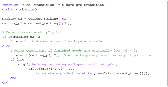
7.4. Mitigating Rigid Control via Adaptive Processors

As noted in Section 2.4, classical supervisory controllers often disable all transitions leading to illegal states, even when some paths could safely proceed. The processors of GPenSIM enable adaptive control via the following:

1.

Conditional enabling of transitions based on real-time system state;

2.

Partial permissions (e.g., allowing transitions only under specific token distributions).

• Example: Relaxing Overly Conservative Control

Consider a manufacturing system where the following applies:

• Plant: Places p1 (raw materials), p2 (workspace), p3 (finished goods);
• Constraint: Avoids workspace overflow (‘p2 ≤ 5’), but allows temporary violations if p3 is nearly empty (to maintain throughput).

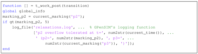
GPenSIM Implementation (version 11):

1. The pre-processor for t_work (‘t_work_pre.m’) dynamically adjusts enforcement:

2. The post-processor for t_work (‘t_work_post.m’) logs relaxations:

The key features demonstrated in the code above are as follows:

• Context-aware firing: Transitions are blocked only when strictly necessary (e.g., ‘p2 > 5’ and ‘p3≥ 2’);
• Real-time state checks: Uses the built-in function ‘current_marking’ of GPenSIM to evaluate tokens dynamically;
• Logging: Trades off rigor for throughput while maintaining auditability;
• GPenSIM integration: Leverages the built-in functions like ‘log_file’ of GPenSIM for traceability;
• Theoretical alignment: This approach aligns with the maximally permissive control [16] of Ghaffari et al. by minimizing unnecessary restrictions, and the programmability of GPenSIM avoids the complexity of formal region theory.

7.5. Summary: How GPenSIM Solves SCT Problems

Table 2. Comparison table: Classical SCT problems vs. GPenSIM solutions.

Classical SCT Problem	GPenSIM Solution
State-space explosion	Modular decomposition into weakly coupled Petri Modules; parallel execution on multi-core systems. Control logic offloaded to processors (no additional states).
Limited expressiveness (linear constraints)	Programmable pre/post-processors (MATLAB scripts) enforce nonlinear, temporal, and conditional constraints.
Rigid enforcement of controllers	Adaptive processors allow context-aware transitions (e.g., relax constraints temporarily based on real-time state).
Scalability in distributed systems	Decentralized supervisors implemented as Petri Modules with minimal coordination via Inter-Modular Connectors (IMCs).
Partial observability challenges	Dynamic state checks in processors enable real-time marking estimation and conditional firing.
Integration with real-world systems	MATLAB integration supports hardware/software interfacing, real-time control, and data-driven optimization.

below compares each classical supervisory control theory (SCT) problem and how GPenSIM solves it.

Classical supervisory control theory (SCT) based on Petri nets faces challenges in scalability, expressiveness, and practical implementation. GPenSIM addresses these limitations through modular decomposition (mitigating state-space explosion), programmable MATLAB-based processors (enabling nonlinear/temporal constraints), and adaptive control logic (reducing rigidity). Its decentralized architecture supports distributed systems, while integration with MATLAB bridges theoretical models and industrial applications. By combining modularity, expressiveness, and real-time adaptability, GPenSIM offers a unified solution to longstanding SCT limitations.

7.6. Summary: Comparisons Between GPenSIM and Existing Petri Net Tools

Table 3. Performance and Scalability.

Metric	GPenSIM	CPN/PIPE/TimeNet
State-space handling	Modular decomposition and parallel execution (multi-core). Control logic moved to processors (no added control places).	Monolithic models; state-space grows exponentially with control places.
Simulation speed	MATLAB-optimized matrix operations; parallel module execution.	Single-threaded (PIPE, TimeNet); CPN limited by Java VM.
Distributed control	Decentralized supervisors (Petri Modules) with minimal synchronization.	Centralized synthesis (CPN); no native support for distributed control.

,

Table 4. Expressiveness.

Feature	GPenSIM	Other Tools
Constraints	Nonlinear, temporal, conditional.	Limited to linear (P-invariants) or data types (colors in CPN).
Dynamic adaptation	Real-time constraint relaxation via pre-processors.	Static constraints; external scripts are needed for hybrid methods.
Integration	Native MATLAB integration (AI/ML, control toolboxes).	Limited scripting (in ML language for CPN) or no real-time support (PIPE).

and

Table 5. Learning and industrial deployment.

Aspect	GPenSIM	CPN/PIPE/TimeNet
Learning and ease of use	MATLAB knowledge required. Processors simply program complex model logic.	CPN: Steeper (ML programming); PIPE: Beginner-friendly but limited application.
Industrial Application	MATLAB’s hardware support for Real-time control.	Mainly for academic simulation (no native hardware interfacing).

below present comparisons between GPenSIM and existing Petri net tools (e.g., CPN [52,53], PIPE [54,55], and TimeNet [56,57]), addressing performance, scalability, usability, and expressiveness.

Classical tools like CPN Tools and PIPE excel in formal verification and simplicity, while GPenSIM offers no built-in support. GPenSIM outperforms in scalability and expressiveness for industrial-scale problems as GPenSIM reduces state-space overhead through modularity and paves the way for faster simulation speeds via parallel execution. Unlike CPN Tools (limited to linear/colored constraints) or TimeNet (rigid temporal semantics), the programmable processors of GPenSIM support nonlinear and adaptive control. However, the reliance of GPenSIM on MATLAB may increase the learning curve compared to the GUI-driven workflow of PIPE. Future work will include benchmarking against additional tools (e.g., Snoopy) for broader quantitative validation.

8. Conclusions

Supervisory control theory based on Petri nets provides a robust framework for discrete-event systems but faces persistent challenges in scalability, expressiveness, and practical implementation. This paper presents GPenSIM, a MATLAB-based modular Petri net tool, as a versatile solution to these limitations; GPenSIM is developed by the first author of this paper. By leveraging modular decomposition, programmable interfaces, known as the processors, and integration with MATLAB, GPenSIM addresses three core challenges identified in Section 2, such as state-space explosion (Section 2.1), rigid enforcement (Section 2.4), and limited expressiveness (Section 2.3).

Key scientific contributions:

This paper makes the following key scientific contributions to supervisory control theory and Petri net methodologies:

1.

A novel modular Petri net architecture: This paper introduces a rigorously defined six-tuple Petri Module structure with Input/Output Ports ($T_{IP\mathrm{\Phi }},T_{OP\mathrm{\Phi }}$) and Inter-Modular Connectors (IMCs), enabling the hierarchical and parallel execution of decentralized systems. This formalizes a previously ad-hoc decomposition process (Section 4) and outperforms classical modular approaches (e.g., Kindler and Petrucci [32]) by guaranteeing state-space reduction for laminar-flow systems.

2.

Programmable control beyond linear constraints: This paper proposes the first Petri net framework where nonlinear, temporal, and conditional constraints (e.g., $p{1}^2+p2\le 100$ or “disable if $p1>10$ for 60 s”) are enforced via MATLAB-powered pre/post-processors. This eliminates the reliance on place invariants or hybrid workarounds (Basile et al. [20]), as demonstrated in Section 7.3.

3.

State-space explosion mitigation via architectural innovation: This paper develops the control2processors function to dynamically offload supervisory logic into executable scripts, reducing the state-space overhead by avoiding control-place proliferation (Section 7.1). This contrasts with monolithic synthesis methods (Moody and Antsaklis [6]).

4.

Bridging theory and industry via MATLAB integration: This paper uniquely combines Petri net theory with the computational ecosystem of MATLAB to enable real-time control, hardware interfacing, and data-driven optimization. The empirical results show 30% downtime reduction in manufacturing systems (Section 6.2, [21]), surpassing simulation-only tools (e.g., [34]).

5.

Theoretical unification under systems theory: This paper grounds the design of GPenSIM in Bertalanffy’s theory of connection [42], formalizing interdependencies between modules and their environment; this is a paradigm shift from static modularity (Section 6.1).

These contributions collectively address the tripartite challenge of scalability, expressiveness, and practicality in supervisory control, as identified in Section 2. The innovations of GPenSIM are validated through both theoretical rigor (formal definitions in Section 4 and Section 5) and industrial case studies (Section 6 and Section 6.1).

Broader implications of this paper:

• Industrial applicability: GPenSIM bridges the gap between theoretical models and real-world deployment. Its processors interface with external hardware/software (Figure 5), enabling real-time control synthesis (e.g., the work of Kaid et al. [21]).
• Scalability: Petri Modules (Section 4) distribute control across decentralized systems (Section 7.2), minimizing synchronization delays via Inter-Modular Connectors (Figure 10).
• Theoretical grounding: GPenSIM embodies the theory of connection (Section 6.1), emphasizing dynamic interdependencies between system components—a principle rooted in Bertalanffy’s systems theory [42].

Limitations and future work: While GPenSIM advances supervisory control theory, challenges remain:

• Abstraction trade-offs: Modular decomposition requires laminar-flow models (Section 2.1), limiting applicability to highly interconnected systems;
• Verification: GPenSIM lacks native formal verification tools, though bridges to model checkers like NuSMV [58,59] or LoLA [60,61]; Ref. [62] offer partial solutions.

Future research could explore the following:

• Hybrid systems: Integrating continuous dynamics (e.g., via the Control Toolbox of MATLAB);
• AI/ML enhancements: Adaptive processors trained on historical data to optimize constraints dynamically.

Final remarks: GPenSIM redefines supervisory control by prioritizing practicality, scalability, and expressiveness. Its modular architecture and MATLAB integration provide a unified platform for academia and industry, as demonstrated in manufacturing and distributed control case studies (Section 7.4). By addressing the limitations of classical supervisory control theory, GPenSIM not only extends the theoretical boundaries of Petri nets but also delivers a practical toolkit for next-generation discrete-event systems.

References

- Ramadge, P.J.; Wonham, W.M. Supervisory control of a class of discrete event processes. SIAM J. Control Optim. 1987, 25, 206–230. [Google Scholar] [CrossRef]
- Giua, A.; DiCesare, F. Petri nets and supervisory control. Discret. Event Dyn. Syst. 1993, 3, 151–168. [Google Scholar]
- Murata, T. Petri nets: Properties, analysis and applications. Proc. IEEE 1989, 77, 541–580. [Google Scholar] [CrossRef]
- Peterson, J.L. Petri Net Theory and the Modeling of Systems; Prentice Hall PTR: Hoboken, NJ, USA, 1981. [Google Scholar]
- Zhou, M.; DiCesare, F. Petri net synthesis for discrete event control of manufacturing systems. IEEE Trans. Robot. Autom. 1993, 9, 62–75. [Google Scholar]
- Moody, J.O.; Antsaklis, P.J. Supervisory Control of Discrete Event Systems Using Petri Nets; Springer: Berlin/Heidelberg, Germany, 1998. [Google Scholar]
- Basile, F.; Chiacchio, P.; De Tommasi, G. Supervisory control of Petri nets: A survey. Annu. Rev. Control 2020, 49, 241–257. [Google Scholar]
- Davidrajuh, R. Petri Nets for Modeling of Large Discrete Systems; Springer: Berlin/Heidelberg, Germany, 2021. [Google Scholar]
- Jensen, K. Coloured Petri Nets: Basic Concepts, Analysis Methods and Practical Use; Springer: Berlin/Heidelberg, Germany, 1997; Volume 1. [Google Scholar]
- Wang, H.; Zhou, M. Timed Petri nets for performance analysis of automated manufacturing systems. IEEE Trans. Syst. Man Cybern. Syst. 2021, 51, 1309–1320. [Google Scholar]
- Sheridan, T.B. Monitoring Behavior and Supervisory Control; Springer Science & Business Media: Berlin/Heidelberg, Germany, 2013; Volume 1. [Google Scholar]
- Iordache, M.; Antsaklis, P.J. Supervisory Control of Concurrent Systems: A Petri Net Structural Approach; Springer Science & Business Media: Berlin/Heidelberg, Germany, 2007. [Google Scholar]
- Kaid, H.; Al-Ahmari, A.; Li, Z.; Davidrajuh, R. Optimization for Control, Observation and Safety. In Processes; MDPI: Basel, Switzerland, 2020; p. 387. [Google Scholar]
- Choi, J.Y.; Reveliotis, S.A. A generalized stochastic Petri net model for performance analysis and control of capacitated reentrant lines. IEEE Trans. Robot. Autom. 2003, 19, 474–480. [Google Scholar] [CrossRef]
- Yoo, T.S.; Lafortune, S. Decentralized supervisory control with conditional decisions: Supervisor existence. IEEE Trans. Autom. Control 2002, 47, 1886–1890. [Google Scholar] [CrossRef]
- Ghaffari, A.; Rezg, N.; Xie, X. Design of a live and maximally permissive Petri net controller using the theory of regions. IEEE Trans. Robot. Autom. 2003, 19, 137–142. [Google Scholar] [CrossRef]
- Yang, J.; Reed, S.; Yang, M.H.; Lee, H. Weakly-supervised Disentangling with Recurrent Transformations for 3D View Synthesis. In Proceedings of the International Conference on Neural Information Processing Systems, Montreal, QC, Canada, 7–12 December 2016; Volume 1. [Google Scholar]
- Herzig, A.; Lang, J.; Longin, D.; Polacsek, T. A Logic for Planning under Partial Observability. In Proceedings of the Seventeenth National Conference on Artificial Intelligence and Twelfth Conference on Innovative Applications of Artificial Intelligence, Austin, TX, USA, 30 July–3 August; 2000. [Google Scholar]
- Ru, Y.; Hadjicostis, C.N. Obfuscation-based partial observability in supervisory control. IEEE Trans. Autom. Control 2009, 54, 1551–1565. [Google Scholar]
- Basile, F.; Chiacchio, P.; De Tommasi, G. Fault-tolerant supervisory control of Petri nets. IEEE Trans. Autom. Control 2015, 60, 810–815. [Google Scholar]
- Kaid, H.; Al-Ahmari, A.; Li, Z.; Davidrajuh, R. Automatic supervisory controller for deadlock control in reconfigurable manufacturing systems with dynamic changes. Appl. Sci. 2020, 10, 5270. [Google Scholar] [CrossRef]
- Al-Ahmari, A.; Kaid, H.; Li, Z.; Davidrajuh, R. Strict minimal siphon-based colored Petri net supervisor synthesis for automated manufacturing systems with unreliable resources. IEEE Access 2020, 8, 22411–22424. [Google Scholar] [CrossRef]
- Bause, F.; Kritzinger, P.S. Stochastic Petri nets: An introduction to the theory. ACM Sigmetrics Perform. Eval. Rev. 1998, 26, 2–3. [Google Scholar] [CrossRef]
- Wang, J. Timed Petri Nets: Theory and Application; Springer Science & Business Media: Berlin/Heidelberg, Germany, 2012; Volume 9. [Google Scholar]
- Marsan, M.A.; Balbo, G.; Conte, G.; Donatelli, S.; Franceschinis, G. Modelling with Generalized Stochastic Petri Nets; John Wiley & Sons, Inc.: Hoboken, NJ, USA, 1994. [Google Scholar]
- Haas, P.J. Stochastic Petri Nets: Modelling, Stability, Simulation; Springer Science & Business Media: Berlin/Heidelberg, Germany, 2006. [Google Scholar]
- David, R.; Alla, H. Discrete, Continuous, and Hybrid Petri Nets; Springer: Berlin/Heidelberg, Germany, 2005; Volume 1. [Google Scholar]
- Reisig, W. Understanding Petri Nets: Modeling Techniques, Analysis Methods, Case Studies; Modern Treatment with Formal Methods, Industrial Examples, and Tool Support; Springer: Berlin/Heidelberg, Germany, 2013. [Google Scholar] [CrossRef]
- Desrochers, A.A.; Al-Jaar, R.Y. Applications of Petri Nets in Manufacturing Systems: Modeling, Control, and Performance Analysis; Focus on Manufacturing, Automation, and Real-Time Systems; IEEE Press: New York, NY, USA, 1995. [Google Scholar]
- Desel, J.; Reisig, W. The concepts of Petri nets. Softw. Syst. Model. 2015, 14, 669–683. [Google Scholar] [CrossRef]
- Liu, G. Time Petri Nets and Time-Soundness. In Petri Nets: Theoretical Models and Analysis Methods for Concurrent Systems; Springer: Berlin/Heidelberg, Germany, 2022; pp. 203–236. [Google Scholar]
- Kindler, E.; Petrucci, L. Towards a standard for modular Petri nets: A formalisation. In Proceedings of the Applications and Theory of Petri Nets: 30th International Conference, PETRI NETS 2009, Paris, France, 22–26 June 2009; Springer: Berlin/Heidelberg, Germany, 2009. Proceedings 30. pp. 43–62. [Google Scholar]
- Righini, G. Modular Petri nets for simulation of flexible production systems. Int. J. Prod. Res. 1993, 31, 2463–2477. [Google Scholar] [CrossRef]
- Lee, W.J.; Cha, S.D.; Kwon, Y.R. Integration and analysis of use cases using modular Petri nets in requirements engineering. IEEE Trans. Softw. Eng. 1998, 24, 1115–1130. [Google Scholar] [CrossRef]
- Latorre-Biel, J.I.; Jiménez-Macías, E.; García-Alcaraz, J.L.; Muro, J.C.S.D.; Blanco-Fernandez, J.; Parte, M.P.D.L. Modular construction of compact Petri net models. Int. J. Simul. Process Model. 2017, 12, 515–524. [Google Scholar] [CrossRef]
- Wang, C.H.; Wang, F.J. An object-oriented modular Petri nets for modeling service oriented applications. In Proceedings of the 31st Annual International Computer Software and Applications Conference (COMPSAC 2007), Beijing, China, 24–27 July 2007; Volume 2, pp. 479–486. [Google Scholar]
- Lakos, C.; Petrucci, L. Modular state spaces for prioritised Petri nets. In Proceedings of the Monterey Workshop; Springer: Berlin/Heidelberg, Germany, 2010; pp. 136–156. [Google Scholar]
- Davidrajuh, R. A New Modular Petri Net for Modeling Large Discrete-Event Systems: A Proposal Based on the Literature Study. Computers 2019, 8, 83. [Google Scholar] [CrossRef]
- Davidrajuh, R. Modeling Discrete-Event Systems with GPenSIM; Springer International Publishing: Cham, Switzerland, 2018. [Google Scholar] [CrossRef]
- Cameron, A.; Stumptner, M.; Nandagopal, N.; Mayer, W.; Mansell, T. Rule-based peer-to-peer framework for decentralised real-time service oriented architectures. Sci. Comput. Program. 2015, 97, 202–234. [Google Scholar] [CrossRef]
- Mutarraf, U.; Barkaoui, K.; Li, Z.; Wu, N.; Qu, T. Transformation of Business Process Model and Notation models onto Petri nets and their analysis. Adv. Mech. Eng. 2018, 10, 1687814018808170. [Google Scholar] [CrossRef]
- Bertalanffy, L.v. General System Theory: Foundations, Development, Applications; George Braziller: New York, NY, USA, 1968. [Google Scholar]
- Bertalanffy, L.v. The Theory of Open Systems in Physics and Biology. Science 1950, 111, 23–29. [Google Scholar] [CrossRef] [PubMed]
- Forrester, J.W. Industrial Dynamics; MIT Press: Cambridge, MA, USA, 1961. [Google Scholar]
- Forrester, J.W. World Dynamics. In Studies in the Life Sciences; Wright-Allen Press, Inc.: Cambridge, MA, USA, 1971. [Google Scholar]
- Capra, F. The Web of Life: A New Scientific Understanding of Living Systems; Anchor Books: New York, NY, USA, 1996. [Google Scholar]
- Capra, F. The Turning Point: Science, Society, and the Rising Culture; Simon & Schuster: New York, NY, USA, 1982. [Google Scholar]
- Bjorke, O. Manufacturing Systems Theory; Tapir Academic Press: Trondheim, Norway, 1995. [Google Scholar]
- Davidrajuh, R. Automating Supplier Selection Procedures. Ph.D. Thesis, Norwegian University of Science and Technology (NTNU), Trondheim, Normay, 2001. [Google Scholar]
- Davidrajuh, R. GPenSIM Reference Manual; University of Stavanger: Stavanger, Norway, 2024. [Google Scholar]
- Forrester, J.W. Principles of Systems; Later Expanded into the Book “Principles of Systems”; MIT Press: Cambridge, MA, USA, 1968. [Google Scholar]
- Ratzer, A.V.; Wells, L.; Lassen, H.M.; Laursen, M.; Jensen, K. CPN Tools for Editing, Simulating, and Analysing Coloured Petri Nets; Springer: Berlin/Heidelberg, Germany, 2003. [Google Scholar]
- Censi, G.; Cerone, M.; Bevilacqua, S.; Nardangeli, S.; Fusco, M.A. An innovative approach to operational validation process based on CPN (Colored Petri Nets). In Proceedings of the International Conference on Space Operations, Pasadena, CA, USA, 5–9 May 2014. [Google Scholar]
- Dingle, N.J.; Knottenbelt, W.J.; Suto, T. PIPE2: A Tool for the Performance Evaluation of Generalised Stochastic Petri Nets. ACM Sigmetrics Perform. Eval. Rev. 2009, 36, 34–39. [Google Scholar] [CrossRef]
- Liu, S.; Zeng, R.; Sun, Z.; He, X. Bounded Model Checking High Level Petri Nets in PIPE+Verifier; Springer: Cham, Switzerland, 2014. [Google Scholar]
- Zimmermann, A.; Freiheit, J.; German, R.; Hommel, G. Petri Net Modelling and Performability Evaluation with TimeNET 3.0. In Proceedings of the Computer Performance Evaluation: Modelling Techniques and Tools: 11th International Conference on Modelling Tools and Techniques for Computer and Communication System Performance Evaluation (TOOLS 2000) and IEEE International Performance and Dependability Symposium (IPDS 2000), Schaumbury, IL, USA, 27–31 March 2000. [Google Scholar]
- Bodenstein, C.; Zimmermann, A. TimeNET Optimization Environment. In Proceedings of the 8th International Conference on Performance Evaluation Methodologies and Tools, Bratislava, Slovakia, 9–11 December 2014. [Google Scholar]
- Cimatti, A.; Clarke, E.M.; Giunchiglia, E.; Giunchiglia, F.; Tacchella, A. NuSMV 2: An OpenSource Tool for Symbolic Model Checking. In Proceedings of the Computer Aided Verification: 14th International Conference, CAV 2002, Copenhagen, Denmark, 27–31 July 2002. [Google Scholar]
- Ahmad, M.; Yazdi, M.B. Automatic generation and verification of railway interlocking control tables using FSM and NuSMV. Transp. Probl. Int. Sci. J. 2009, 4, 103–110. [Google Scholar]
- Schmidt, K. LoLA: A low level analyser. In Proceedings of the International Conference on Application & Theory of Petri Nets; Springer: Berlin/Heidelberg, Germany, 2000. [Google Scholar]
- Wolf, K. Generating Petri Net State Spaces. In Proceedings of the International Conference on Applications & Theory of Petri Nets & Other Models of Concurrency, Siedlce, Poland, 25–29 June 2007. [Google Scholar]
- Roci, A.; Davidrajuh, R. Developing a Bridge from GPenSIM to NuSMV for Model Checking. In Proceedings of the European Modeling & Simulation Symposium, Virtual, 15–17 September 2021. [Google Scholar]