Abstract
Aiming at the problem that the aggravation of the wheel tread wear of high-speed trains leads to the deterioration of train operation performance and an increase in re-profiling times, a multi-objective data-driven optimization design method for the wheel profile is proposed. Firstly, the chaotic map is introduced into the population initialization process of the golden jackal algorithm. In the later stage of the algorithm iteration, random disturbance is introduced with optimization algebra as the switching condition to obtain an improved optimization algorithm, and the performance index of the optimization algorithm is verified to be superior to other algorithms. Secondly, the improved multi-objective optimization algorithm and data-driven model are used to optimize the tread coordinates and obtain an optimized profile. The vehicle dynamics performance of the optimized profile and the wheel wear evolution after long-term service are compared. The results show that the tread wear index of the left and right wheels in a straight line is reduced by 62.4% and 62.6%, respectively, and the wear index of the left and right wheels in a curved line is reduced by 26.5% and 5.5%, respectively. The stability and curve passing performance of the optimized profile are improved. Under the long-term service conditions of the train, the wear amount of the optimized profile is greatly reduced. After the wear prediction of 200,000 km, the wear amount of the optimized profile is reduced by 60.1%, and it has better curve-passing performance.
1. Introduction
Reducing wheel wear can effectively improve the performance of the wheel–rail system, extend the maintenance cycle of wheels, and thereby reduce the maintenance costs of high-speed trains. Currently, optimizing the wheel–rail profile is one of the primary methods for reducing wheel wear. Through profile optimization, the contact relationship between the wheel and the rail can be made more stable, thereby enhancing the operational safety, smoothness, and ride comfort of the train [1,2,3]. Early researchers adopted conical tread designs, but this design often led to two-point contact between the wheel flange and rail during wheel–rail matching, resulting in significant wear. Heumann [4] proposed using wear-shaped treads as an alternative to conical treads, and subsequently, various countries began conducting research on wear-shaped tread designs. Early wear-type tread designs primarily relied on empirical methods and trial-and-error approaches, which were inefficient, costly, and highly dependent on data and experience. With the development of computers and numerical calculations, many researchers have conducted wheel–rail profile optimization design using computers and numerical calculations as tools. Heller [5] considered three aspects of performance—curve-passing performance, wheel–rail wear, and vehicle stability—in wheel tread design and developed an optimization design program for a single-arc profile. Shevtsov [6,7] used multi-point approximation technology based on response surface fitting, with rolling circle radius difference as the design objective, optimized the contour design, improved contour matching and dynamic performance, and reduced wheel–rail wear. Zhang Jian [8,9] designed a wheel contour matching CHN60 using the contour extension method and further combined the wheel–rail contour contact state with equivalent taper to improve the rail profile. Polach [10] proposed a wheel profile design method based on tread wear width and equivalent taper objectives. Gerlici [11] developed a method for designing railway wheel and rail head profiles based on geometric characteristics, optimizing geometric shapes to enhance contact characteristics and wear resistance between wheels and tracks. Igensti [12] designed an optimized wheel profile using multi-body modeling and wear assessment models and designed an optimized wheel profile.
Additionally, the Rosenbrock function, proposed by Rosenbrock [13], is widely used as a benchmark in optimization due to its nonlinear, multivariable coupling and narrow valley characteristics. It is commonly employed to evaluate the convergence capability and robustness of optimization algorithms in complex landscapes. Seyedali Mirjalili [14] introduced the Grey Wolf Optimizer (GWO), which has demonstrated strong global search ability and convergence performance across a variety of optimization problems. And railway researchers have conducted extensive studies on wheel–rail vehicle optimization design using intelligent algorithms. Persson [15] proposed a method for optimizing railway profiles using genetic algorithms, selecting the optimal profile by simulating and evaluating the performance of different profiles. Furthermore, Novales and Iwnicki [16,17] also employed genetic algorithms to establish wheel profile optimization design models with objectives such as wheel–rail wear and wheel–rail contact fatigue damage. Choi [18] utilized the Non-Dominated Sorting Genetic Algorithm II (NSGA-II) to optimize flange wear and surface fatigue. The optimized design achieved better performance than the initial wheel profile. Zeng [19] established a parameterized model for rail surface modeling and modification using weighted non-uniform rational B-spline curves, obtained the optimal weighting factors via the NSGA-II, and derived the corresponding optimal pre-grinding profile. The maximum contact stress was significantly reduced after optimization. Cui [20] employed a particle swarm optimization algorithm to optimize the LMA and LMD tread profiles. Lin [21] also used this algorithm to optimize a thin flange tread profile based on the LM profile. Ye [22] introduced two design variables and an empirical formula to propose a rotary-scaling fine-tuning method for fine-tuning the traditional wheel profile and applied it in contour optimization design to generate alternative contours. Qi [23] conducted contour optimization design for metro vehicles with the aim of reducing wheel–rail wear.
In the aforementioned literature, various types of intelligent optimization algorithms were employed to achieve wheel tread optimization design, which improved the wheel–rail relationship to some extent and enhanced the dynamic performance of rail vehicles. However, wheel wear was still reflected through wheel–rail wear experiments to establish a wear calculation model, without establishing a mapping relationship between tread parameters and wear. Therefore, this paper proposes a data-driven multi-objective optimization method for high-speed train wheel profiles using neural networks to establish data-driven wheel wear indices and dynamic performance surrogate models. Based on the surrogate models, multiple optimization objectives are calculated, and the improved golden eagle algorithm is used for iterative optimization of the profile coordinates. The study compares the effects of the optimized and unoptimized profiles on train wear performance, dynamic performance, and long-term service performance in straight and curved sections, verifying the feasibility of the method.
2. Model Building
2.1. Vehicle Dynamics Model of High-Speed Trains
This paper uses high-speed trains as an example. For each component in the multi-body model of the vehicle, assuming that the component has n degrees of freedom, the differential equation for its dynamic calculation is shown in Equation (1).
where is the mass matrix, is the damping matrix, is the stiffness matrix, is the system state vector, and is the external excitation force vector.
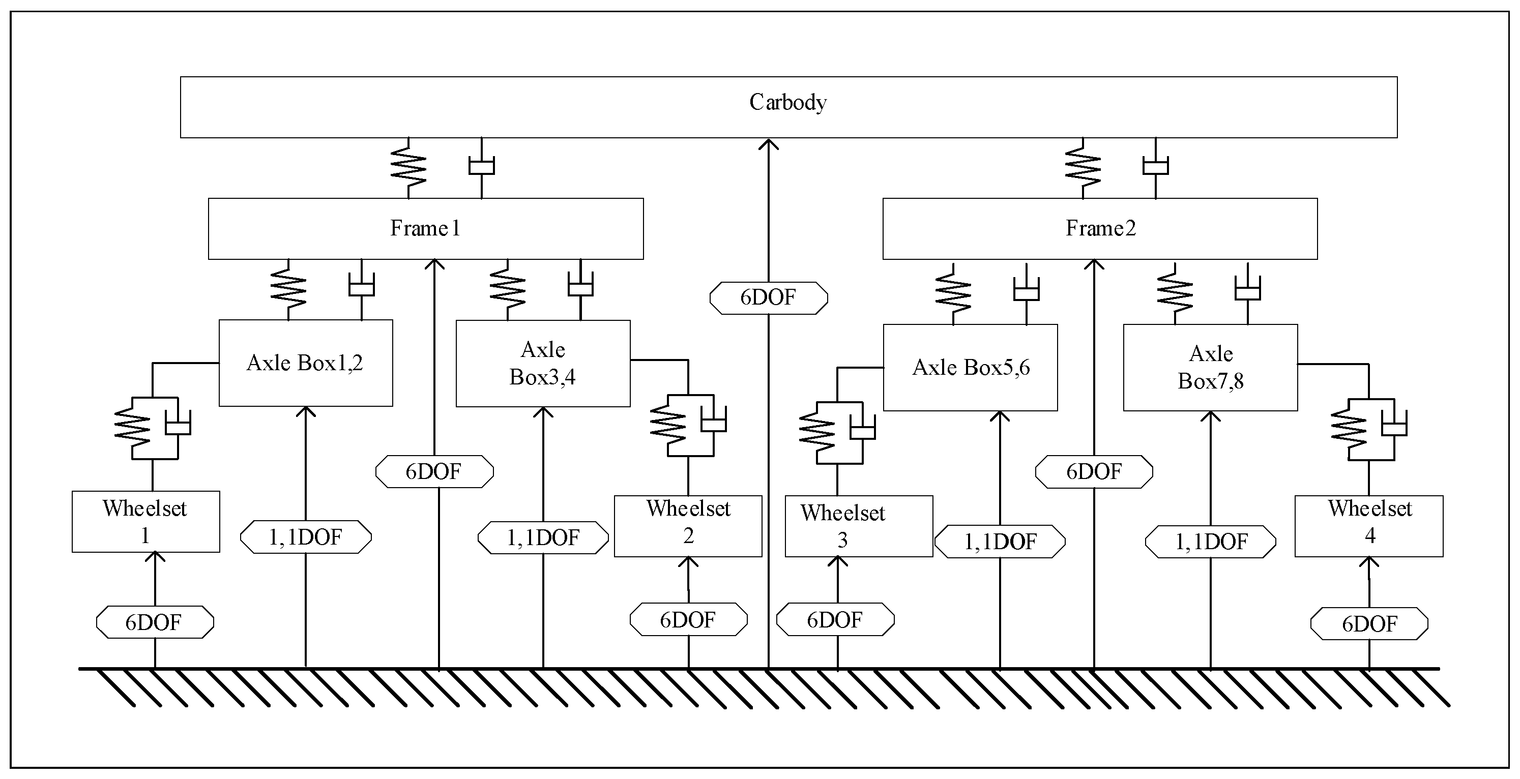
Figure 1 presents the topological layout of the dynamic model for a single trailer coach of a high-speed train. The model is composed primarily of one car body, two bogies, and four wheelsets. The car body, each bogie, and each wheelset are endowed with six degrees of freedom—lateral, vertical, longitudinal, roll, pitch, and yaw—whereas each axle box has a single degree of freedom. As summarized in Table 1, the complete vehicle therefore comprises 50 degrees of freedom in total; “1” denotes a released degree of freedom and “0” denotes a constrained one.
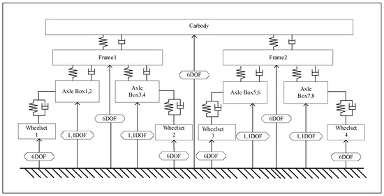
Figure 1.
Topology of the dynamic model for a single trailer car of a high-speed train.

Table 1.
Degree of freedom of vehicle multi-rigid-body model.
2.2. Vehicle Dynamics Model of High-Speed Trains
In this paper, based on the Archard wear model of friction work [24], the model considers the linear relationship between the wear volume and the friction work as follows.
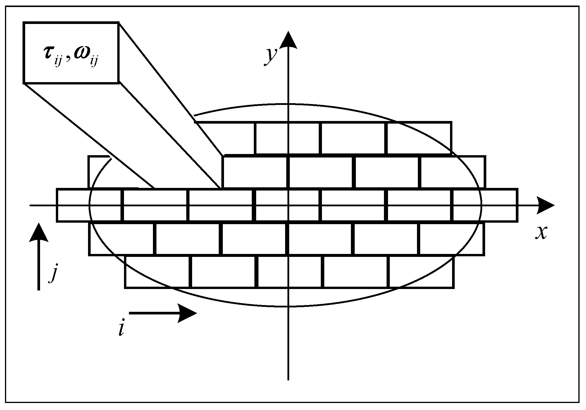
where W is the wear volume of the material, is the accumulated wear coefficient, A is the friction work, P is the friction power, is the tangential stress in the contact unit, is the sliding speed, and F is the contact spot area. In the calculation, the contact patch is regarded as the same plane and discretized into an equal-width rectangle parallel to the x-axis, as shown in Figure 2. In each time integration step , the wear volume of each element in the wheel–rail contact patch is shown in Equation (5):

Figure 2.
Discretization of contact spots.
In the formula, v is the speed of the wheelset, is the creep rate of the center of the contact element, and is the area of the contact element.
3. Optimized Design of Low-Wear Wheel Treads
3.1. Formulation of the RPSTC-GJO Algorithm
To mitigate the tendency of the Golden Jackal Optimization (GJO) algorithm to become trapped in local optima during the later stages of the search—thereby weakening its overall optimization capability—two enhancements are introduced. First, a Sine–Tent–Cosine (STC) chaotic map is embedded in the initialization phase to enrich population diversity and coverage, thus strengthening global exploration. Second, a random-perturbation mechanism is applied in the final search phase to raise the probability of escaping local optima and reaching the true optimum. These modifications yield the Random-Perturbation Sine–Tent–Cosine chaotic Golden Jackal Optimization algorithm (RPSTC-GJO).
3.1.1. Sine–Tent–Cosine Chaotic Map
Chaos is characterized by randomness, ergodicity, and a high sensitivity to initial conditions, making it a popular choice for population initialization. The Tent chaotic map, a piecewise linear two-dimensional mapping, helps distribute initial solutions as uniformly as possible across the search space. Its definition is given in Equation (6).
In Equation (6), the parameter is introduced as a random variable to offset the short periodic cycles and fixed points inherent in the Tent chaotic map. Chaos can generally be classified as either low dimensional or high dimensional. High-dimensional chaotic systems exhibit complex structures, numerous control parameters, and high computational overhead. Low-dimensional chaos, by contrast, features simpler structures and fewer parameters and is easier to implement, yet it suffers from discontinuous chaotic intervals and non-uniform sequence distributions. To reconcile these drawbacks, researchers often construct composite chaotic systems by combining several low-dimensional maps; such systems deliver superior chaotic performance while retaining lower complexity than high-dimensional counterparts. By selecting the control parameter within the Tent map and fusing it with the Sine and Cosine maps, a Sine–Tent–Cosine chaotic map is obtained, whose mathematical form is provided in Equation (7).
where r denotes a uniformly distributed random number in the interval .
3.1.2. Random Perturbation
In the later stages of the GJO search, a random-perturbation mechanism is introduced. Specifically, an additional stochastic term is injected into the position-update equations of both the male and female jackals, forcing them to disperse toward different locations, explore new search trajectories, and thereby improve the probability of discovering a superior optimum. The activation of this perturbation is controlled by the iteration index: once the iteration count reaches the prescribed switching threshold, Equations (8) and (9) are adopted to update the prey’s position relative to the male and female jackals, while Equations (10) and (11) are employed to update the cooperative encirclement model that governs how the two jackals jointly pursue the prey.
where t is the current iteration index; is the prey-position matrix; and denote the positions of the male and female jackals at iteration t, respectively; is a Lévy-distributed random variable; are independent uniform random numbers from the interval ; and specifies the problem-dependent range of the random perturbation. By incorporating this stochastic displacement into the position-update rules, jackals that have become trapped in a local optimum gain the ability to escape and resume a global search for better solutions.
The optimization steps are described in Algorithm 1, and this experiment was conducted on an AMD R5 2600 processor, with a clock speed of 3.4 GHz, 16 GB of memory, Windows 10 64 bit operating system, and Matlab 2020a software environment.
| Algorithm 1: RPSTC-GJO Algorithm (Random-Perturbation Sine–Tent–Cosine Golden Jackal Optimization) |
 |
3.2. Algorithm Validation
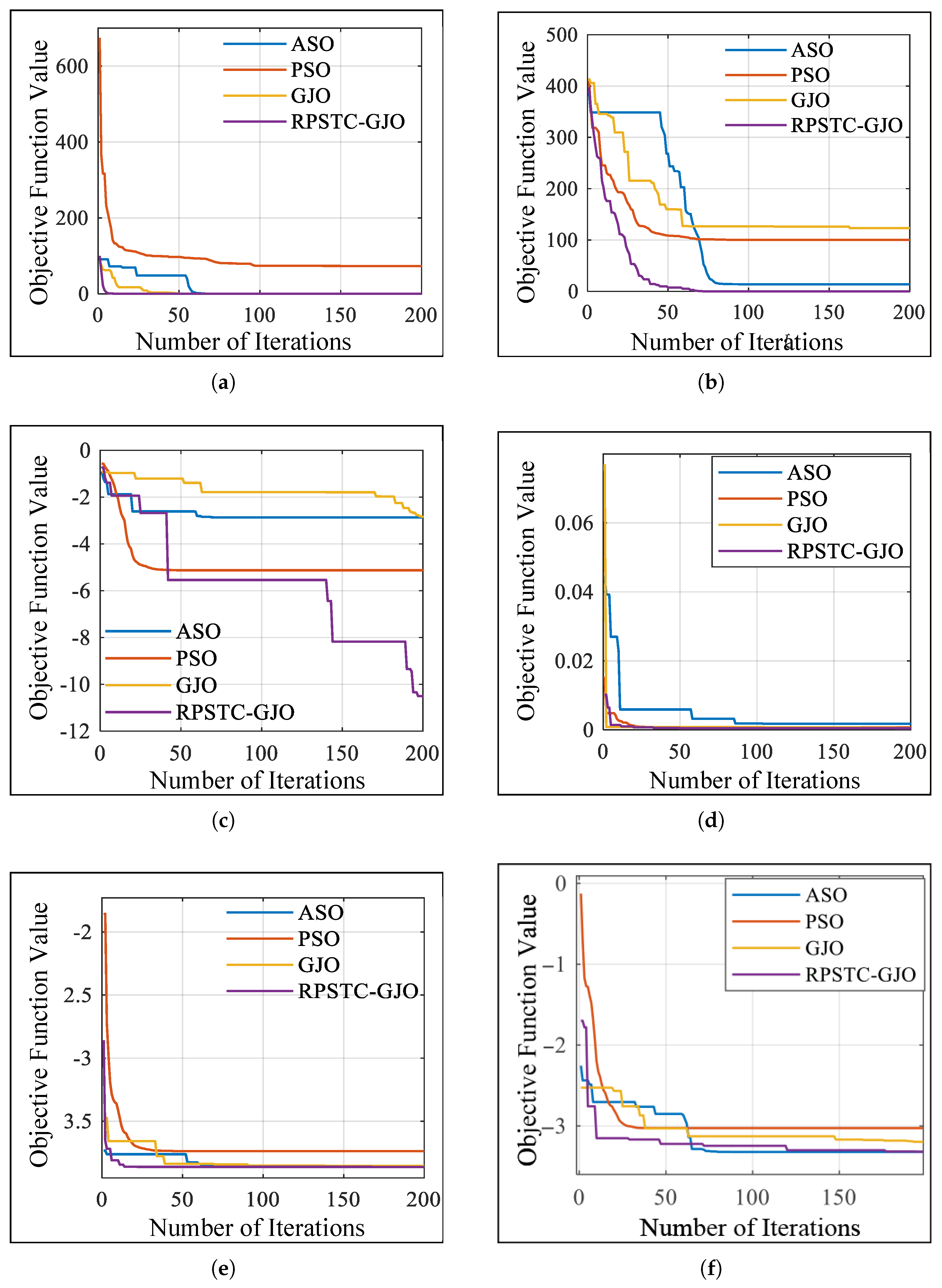
To evaluate the optimization performance of the RPSTC-GJO algorithm, six benchmark test functions (Table 2) were selected. The proposed method was compared with three classical approaches—particle swarm optimization (PSO), atomic search optimization (ASO), and the original Golden Jackal Optimization (GJO) [25,26]. Comparative results obtained on the six benchmark functions are summarized in Figure 3.
Table 2.
Basic parameters of benchmark test functions used for algorithm comparison.
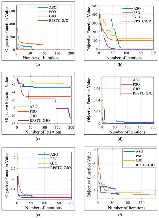
Figure 3.
Fitness convergence curve of standard functions. (a) Benchmark Function . (b) Benchmark Function . (c) Benchmark Function . (d) Benchmark Function . (e) Benchmark Function . (f) Benchmark Function .
Figure 3a plots the evolution of the objective value for the four algorithms when tested on the first benchmark function. It is evident that the initial fitness values of ASO, GJO, and the RPSTC-GJO are markedly better than that of PSO. Moreover, the RPSTC-GJO converges to the optimum more rapidly than the original GJO. Figure 3b presents the iteration curves of the objective value on the second benchmark function. Both GJO and PSO remain trapped in local optima throughout the run. Although ASO converges to a neighborhood of the optimum, it ultimately stagnates, whereas the RPSTC-GJO reaches the optimum faster and more closely than ASO. Figure 3c depicts the performance on the third benchmark function. As the iterations proceed, ASO and PSO become stuck in local minima and fail to escape. The RPSTC-GJO also experiences a temporary stagnation but later jumps out of the local optimum and converges near the global value of −10.5363. Figure 3d shows the results for the fourth benchmark function. GJO starts with a much poorer initial fitness than the other methods; despite its quick early convergence, it remains in a local optimum. The RPSTC-GJO begins with a better initial solution, and although it converges more slowly than GJO in the early phase, it ultimately escapes the local optimum and settles closer to the true optimum. Figure 3e,f illustrate the objective-value trajectories for the fifth and sixth benchmark functions, respectively. Although the RPSTC-GJO does not have the best initial fitness, it exhibits a high convergence rate and consistently reaches the optimum quickly. Even when it sporadically falls into local optima, it manages to escape as iterations continue, thereby approaching the global optimum more closely than the competing algorithms.
3.3. Optimization Design of Low-Wear Wheel Profiles
3.3.1. NURBS Curve-Fitting Process
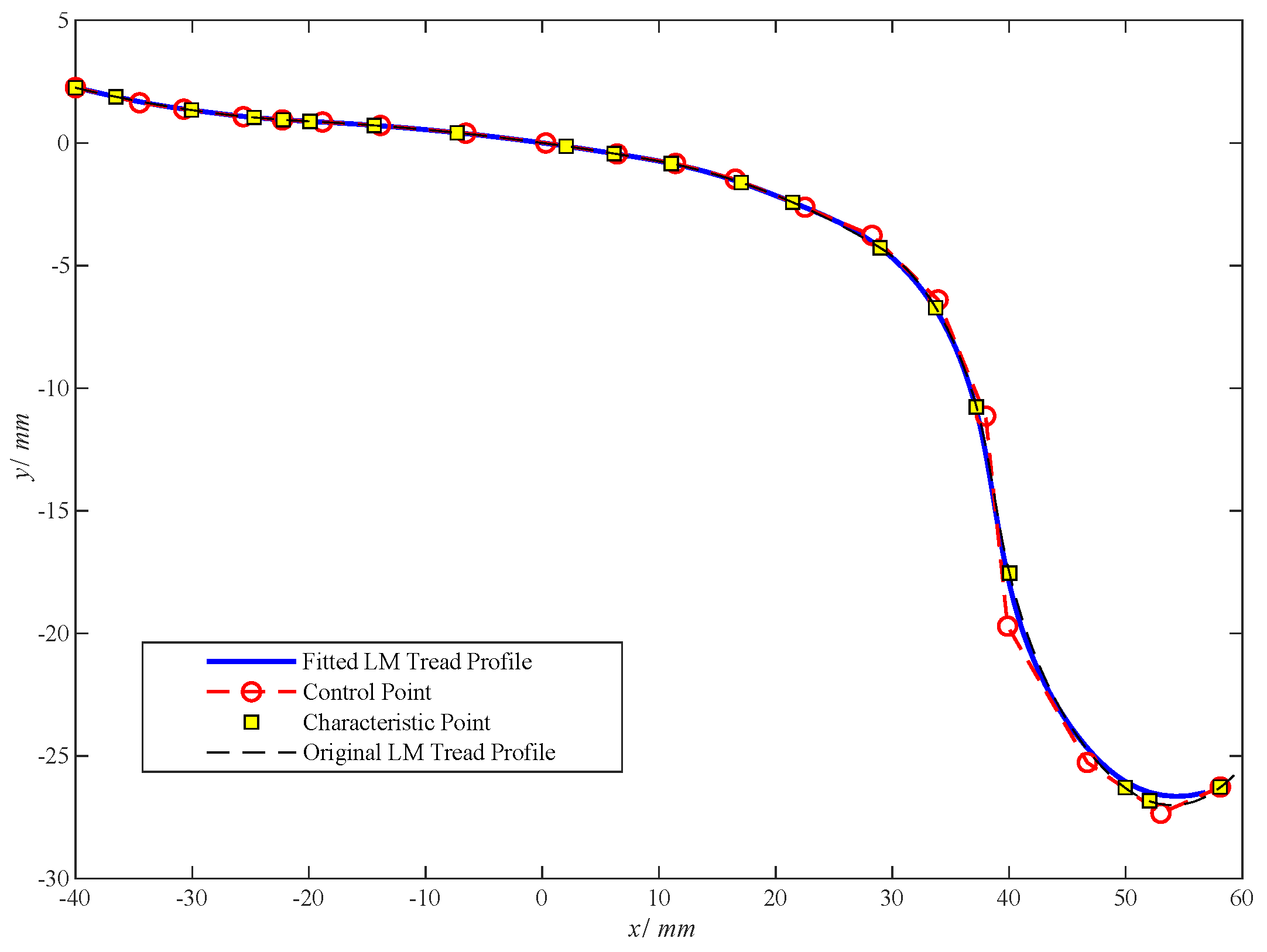
According to the cubic-NURBS curve theory [27], the wheel tread profile is first divided into 19 equal-arc-length segments. A weighting factor is then assigned to each tread point, and the corresponding control vertices are obtained by a matrix-inversion procedure. A larger weight draws the fitted curve closer to its control vertex, whereas a smaller weight pushes the curve farther away. Because the wheel flange is crucial for guiding the vehicle safely along the rail and preventing derailment at high speed, relatively large weights are applied in the flange region. In contrast, wear-evolution studies indicate that the rolling circle and its vicinity constitute the principal wear zone; therefore, smaller weights are used on the tread to widen the optimization range there. Figure 4 compares the control points, the fitted wheel-tread profile, and the standard profile.
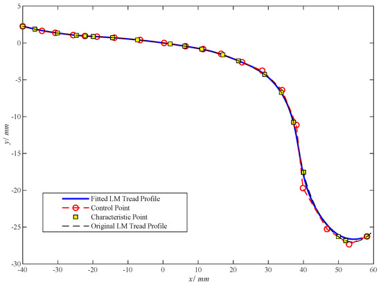
Figure 4.
High-speed train wheel profile fitting diagram.
3.3.2. Objective Function
The axle lateral force H is the algebraic sum of the lateral forces on the left and right wheels of the same wheel set, as given in Equation (12).
where and are the wheel–rail lateral forces acting on the left and right wheels of the wheelset, respectively. An excessive axle lateral force not only inflicts severe damage on the track infrastructure but also poses a serious threat to the running safety of high-speed trains. Hence, in the present optimization study, the axle lateral force of a selected wheelset in a single trailer car is adopted as one of the objective functions.
To assess wheel–rail wear, the Elkins wear index is employed, whose formulation is given in Equation (13).
where and are the longitudinal and lateral creep forces, respectively, and and are the corresponding longitudinal and lateral creepages.
Once the objective functions for the present optimization have been defined, they are combined into a single scalar objective through a weighted-sum method, as formulated in Equation (14).
Equation (14) aggregates the multiple objectives into a single scalar objective, which is subsequently adopted as the target function in the RPSTC-GJO optimization model for iterative computation.
3.3.3. Constraints
To generate a smooth wheel-profile curve that complies with the geometric characteristics of wheel profiles, geometric and boundary constraints are imposed in the optimization procedure. The geometric constraints enforce the monotonicity and convexity/concavity of the fitted curve. In this study, the tread profile measured after 200,000 km of high-speed operation and the as-turned, unworn tread profile are employed as the upper and lower bounds, respectively, as expressed in Equation (15).
where is the vertical coordinate of the t-shape point in the optimization process, and and are the corresponding vertical coordinates of the upper and lower boundary profiles, respectively. As illustrated in Figure 4, the wheel-tread profile from the tread origin to the flange root is monotonic decreasing. Consequently, the first derivative of the fitted curve between shape points 1 and 17 must be negative, as enforced in Equation (16).
Based on the convexity–concavity analysis of the wheel profile, the admissible convex-concave range of the curve is obtained, and its constraint condition is formulated in Equation (17).
3.4. Data-Driven RPSTC-GJO Optimization Computation
3.4.1. Data-Driven Model
Taking the single-trailer dynamical model of a high-speed train as the study object, wheel-wear evolution is predicted under varying operating speeds, accumulated mileages, and curve radii to generate a set of worn tread profiles. Each profile is then fed into the vehicle model to compute key dynamic indicators and wear metrics. The resulting data are consolidated into a dataset, which is used to train an Improved Multi-Layer Extreme Learning Machine (I-ML-ELM) [28]. The trained network establishes a data-driven mapping between the worn tread geometry, the tread wear index, and the axle lateral force of the train.
3.4.2. Optimization Computation
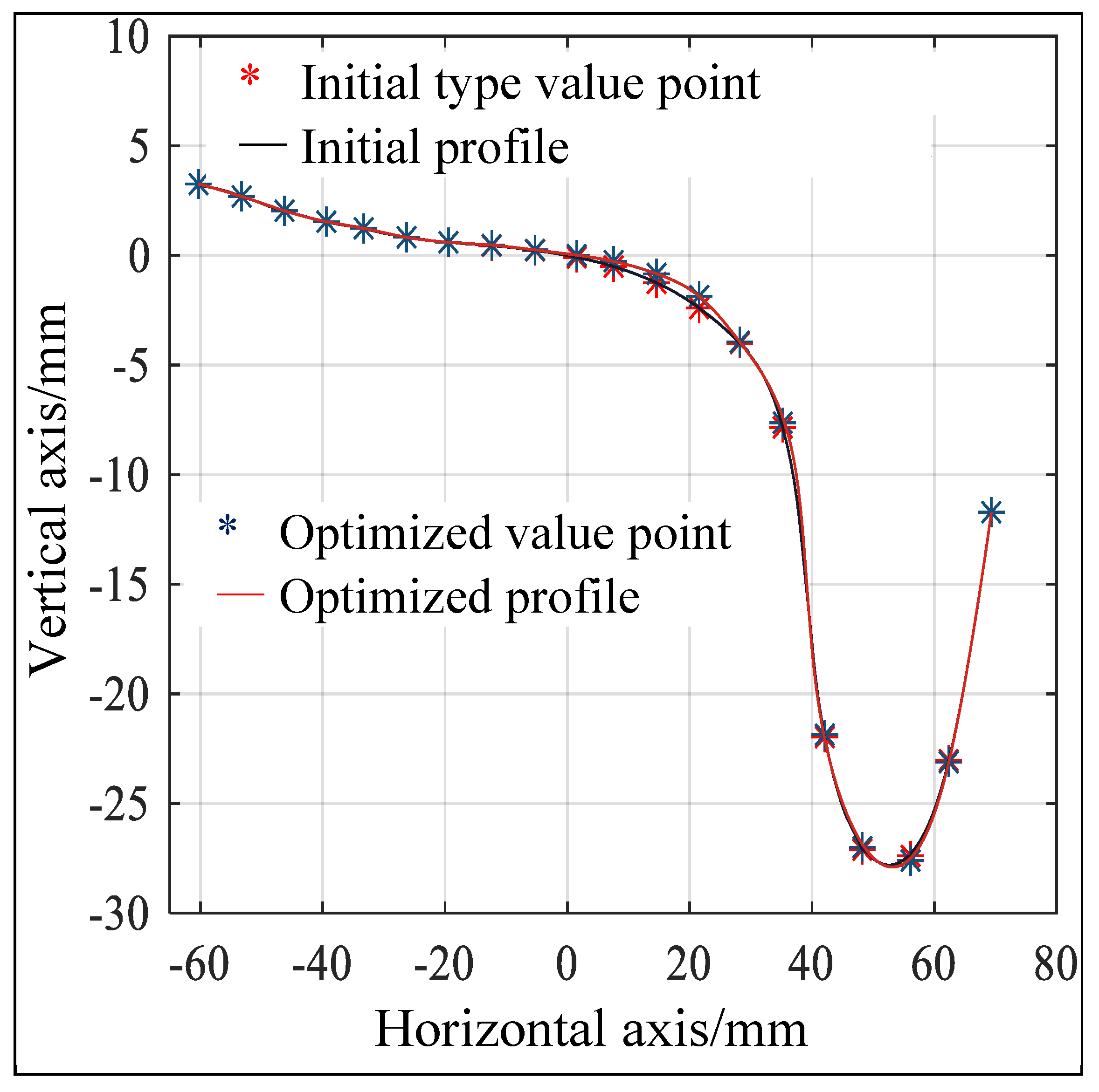
The trained data-driven model is combined with the RPSTC-GJO optimization algorithm to optimize the design of the wheel tread profile. The design process aims to reduce the lateral force on the axle during train operation and the Elkins wear index. Through continuous iteration, prediction, updating, and comparison, the coordinates of the optimized tread profile points are obtained, resulting in lower wheel–rail wear and reduced lateral force on the axle. After 200 iterations of optimization calculations, the optimized wheel tread profile point coordinates were obtained. The optimized profile points were reconstructed using the theory of cubic-NURBS curves, and the fitted wheel tread profile is shown in Figure 5. Before and after tread optimization, the same track conditions were maintained, including 60 N standard rails, a 1435 mm standard gauge, and a 1:40 track bed slope. In the wheel–rail nonlinear contact analysis, the equivalent taper was calculated using the International Union of Railways standard UIC 519 [29] calculation method, with the wheel set lateral displacement set to 3 mm. The calculation results show that the equivalent cone angles before and after optimization are 0.067 and 0.050, respectively, both of which meet the requirements for equivalent cone angles specified in the literature (not exceeding 0.35) [30].

Figure 5.
Comparison of contours before and after optimization.
4. Analysis of Tread Wear and Dynamic Performance
4.1. Analysis of Wheel-Tread Wear Index Under Two Profile Conditions
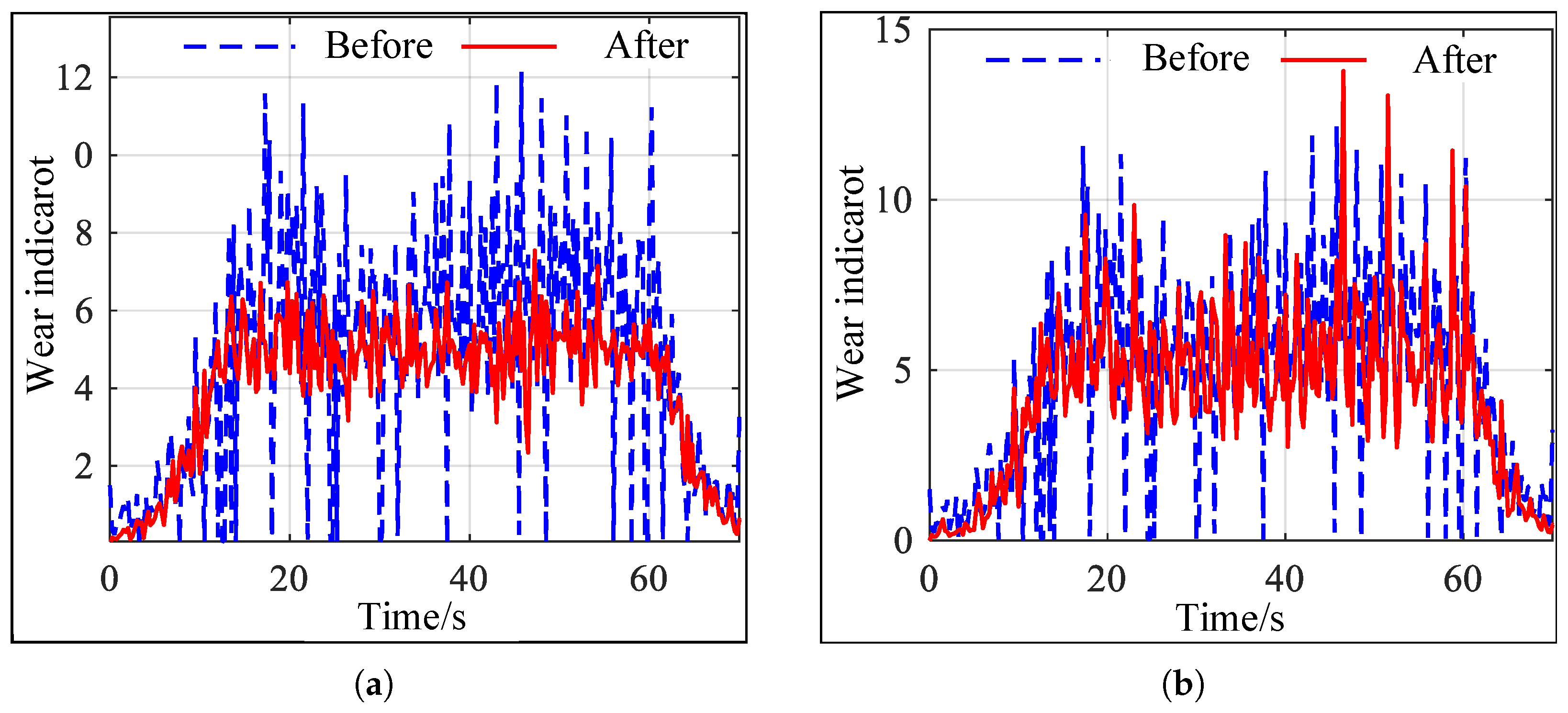
Figure 6 and Figure 7 show the comparison of wheel–rail wear indices for the left and right wheels of a single wheel set when the train is operating on a straight section and a curved section with a radius of 7000 m, respectively, at a speed of 300 km/h. As shown in Figure 6, the optimized profile effectively reduces wheel–rail wear during operation on the straight section. The wear index calculation results for the curved section are shown in Figure 7. As shown in Figure 7a, the wear index of the left wheel of the wheel set is significantly reduced compared to the wear index of the pre-optimized profile. The changes in the wear index of the right wheel can be seen in Figure 7b. Except for a few points where the wear index is higher than that of the initial tread surface, the wear index of the wheels in other areas is significantly reduced.
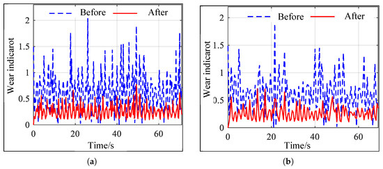
Figure 6.
Comparison of wear indicators before and after straight segment optimization. (a) Comparison of left wheel wear indicators. (b) Comparison of right wheel wear indicators.

Figure 7.
Comparison of wear indicators before and after curve segment optimization. (a) Comparison of left wheel wear indicators. (b) Comparison of right wheel wear indicators.
Table 3 shows the results of calculating the right and left wheel sets’ tread wear indices for trains equipped with two types of treads operating on straight and curved sections of track. On straight sections, the tread wear indices of the left and right wheels decreased by 62.4% and 62.6%, respectively. On curved sections, the wear indices of the left and right wheels decreased by 26.5% and 5.5%, respectively. The optimized profile effectively reduces wheel–rail wear.
Table 3.
Comparison of contour wear indices before and after optimization of different lines.
4.2. Analysis of Vehicle Dynamic Performance Under Two Profile Conditions
4.2.1. Running Stability Analysis of the Vehicle Under Two Profile Conditions
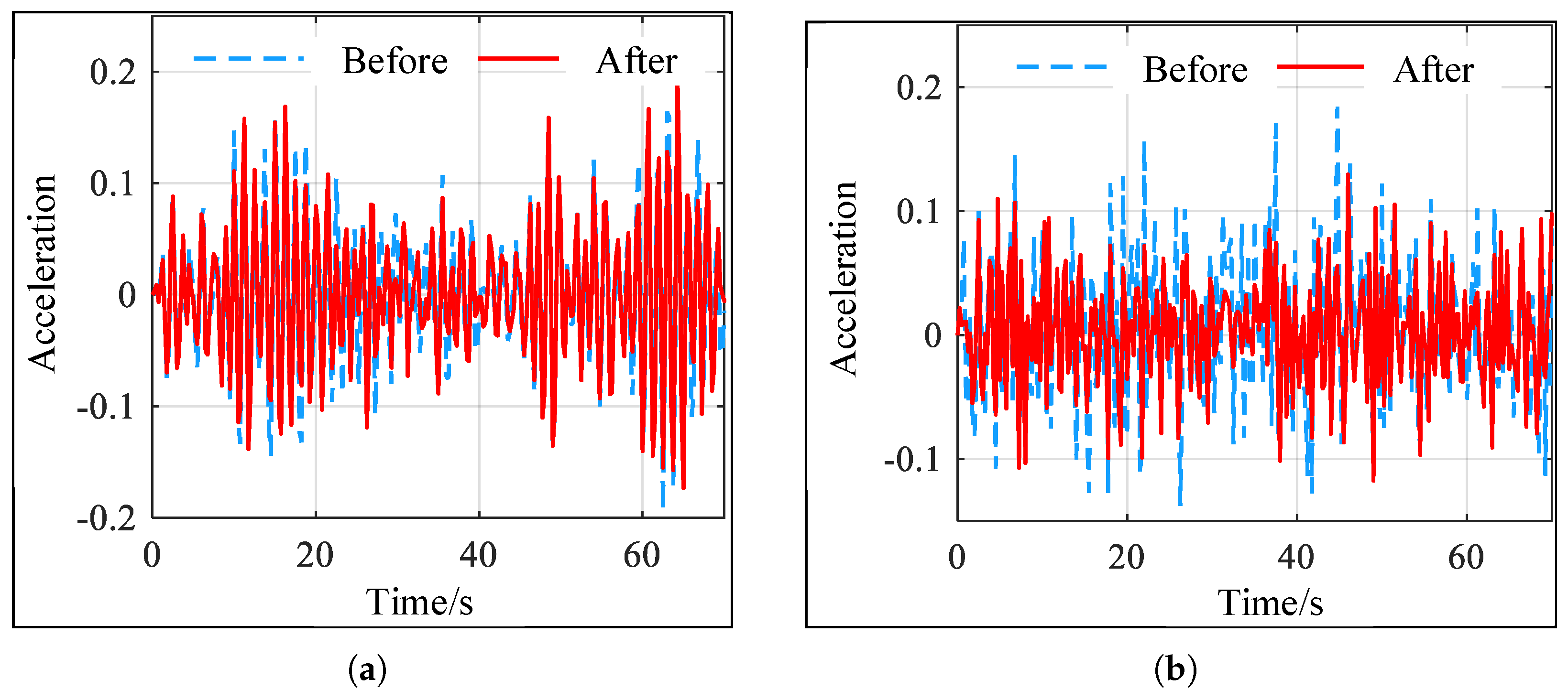
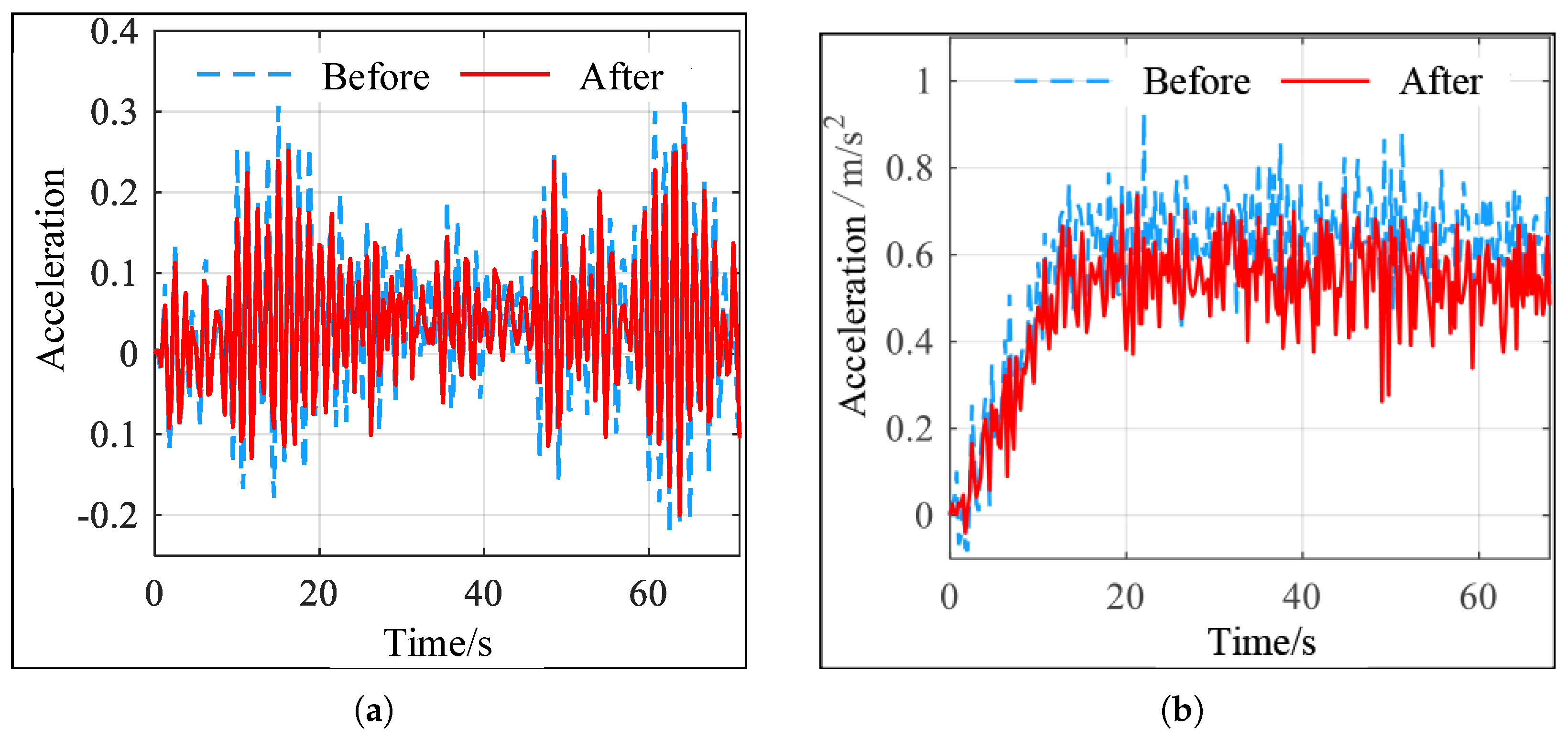
The simulation conditions are the same as those described above. Simulation calculations were performed on the vibration acceleration of car bodies with different wheel profiles on the same type of track. The lateral and vertical vibration acceleration of car bodies when trains with different wheel profiles are running on straight sections are shown in Figure 8, and the lateral and vertical vibration acceleration of car bodies when trains are running on curved sections are shown in Figure 9.

Figure 8.
Comparison of vibration acceleration before and after straight segment optimization. (a) Vertical vibration acceleration. (b) Lateral vibration acceleration.
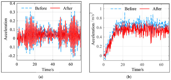
Figure 9.
Comparison of vibration acceleration before and after curve segment optimization. (a) Vertical vibration acceleration. (b) Lateral vibration acceleration.
As shown in Figure 8a, except for a few points, the body vibration acceleration of the train running in a straight line with the optimized contour is smaller than the frame vibration acceleration under the initial contour. As shown in Figure 8b, the lateral vibration acceleration of the train running in a straight line with the optimized contour is significantly lower than that of the train with the initial contour. As shown in Figure 9, the lateral and vertical vibration acceleration of the train body during curved operation with the optimized profile is significantly lower than that of the frame under the initial profile. The corresponding lateral and vertical Sperling indices and maximum vibration acceleration values for the train under different track sections and profiles are shown in Table 4:
Table 4.
Comparison of Sperling index and maximum vibration acceleration before and after optimization.
As shown in Table 4, all values after wheel contour optimization are better than the initial values, and the maximum vertical and lateral vibration acceleration values of the vehicle body equipped with the optimized wheel contour are both lower than those before optimization.
4.2.2. Curving Performance Analysis of the Vehicle Under Two Profile Conditions
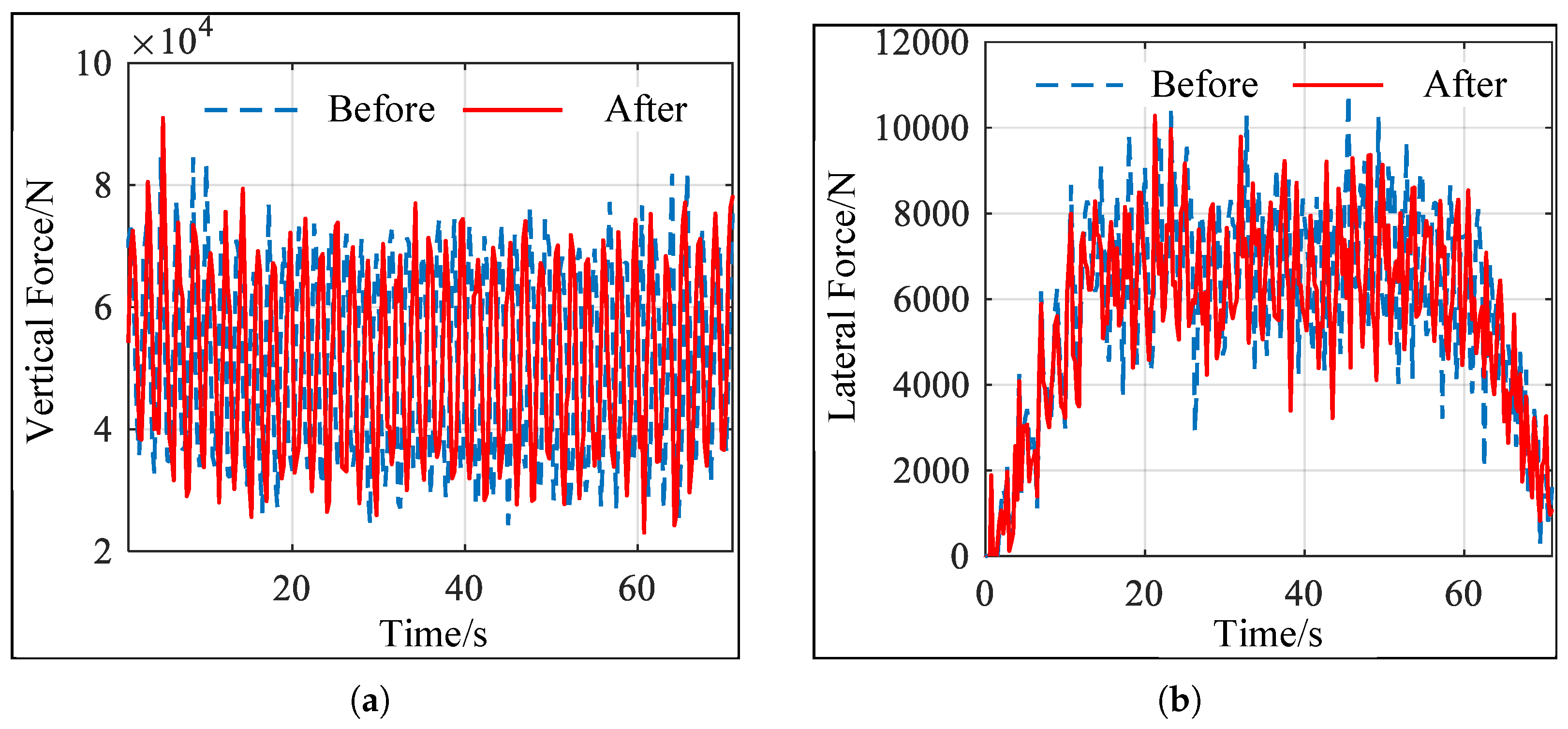
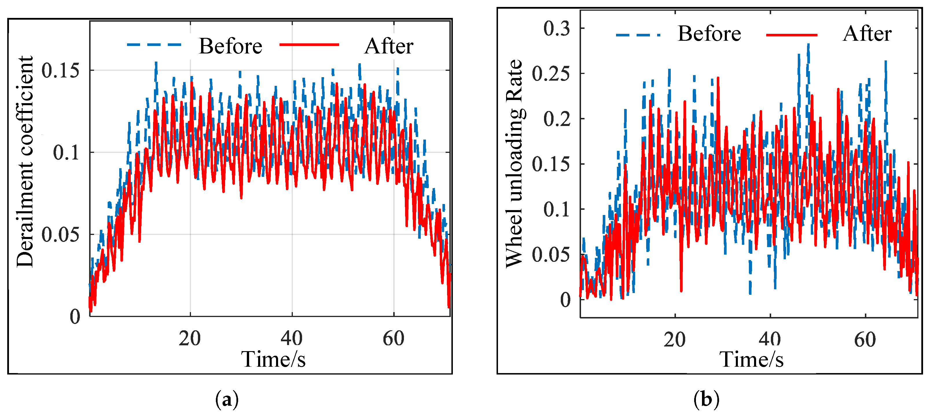
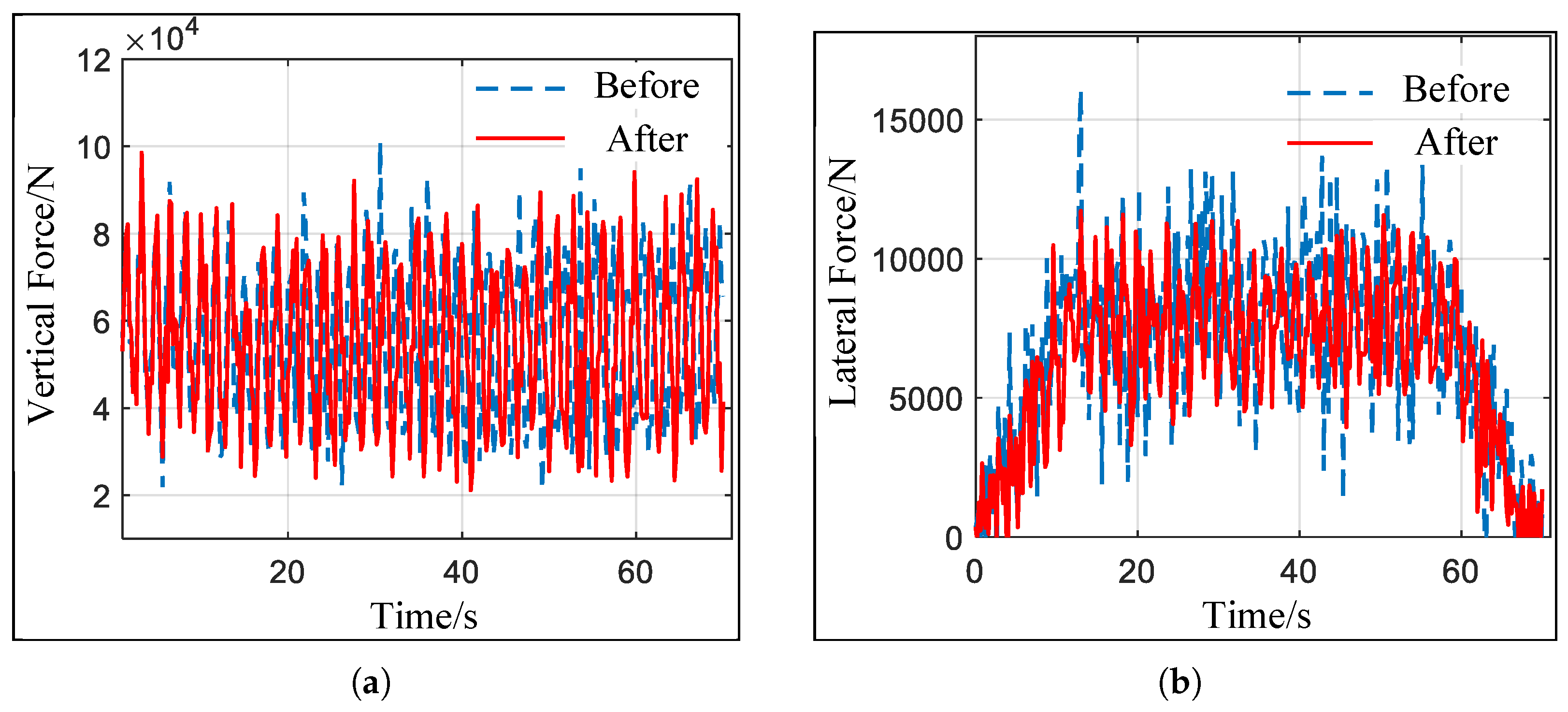
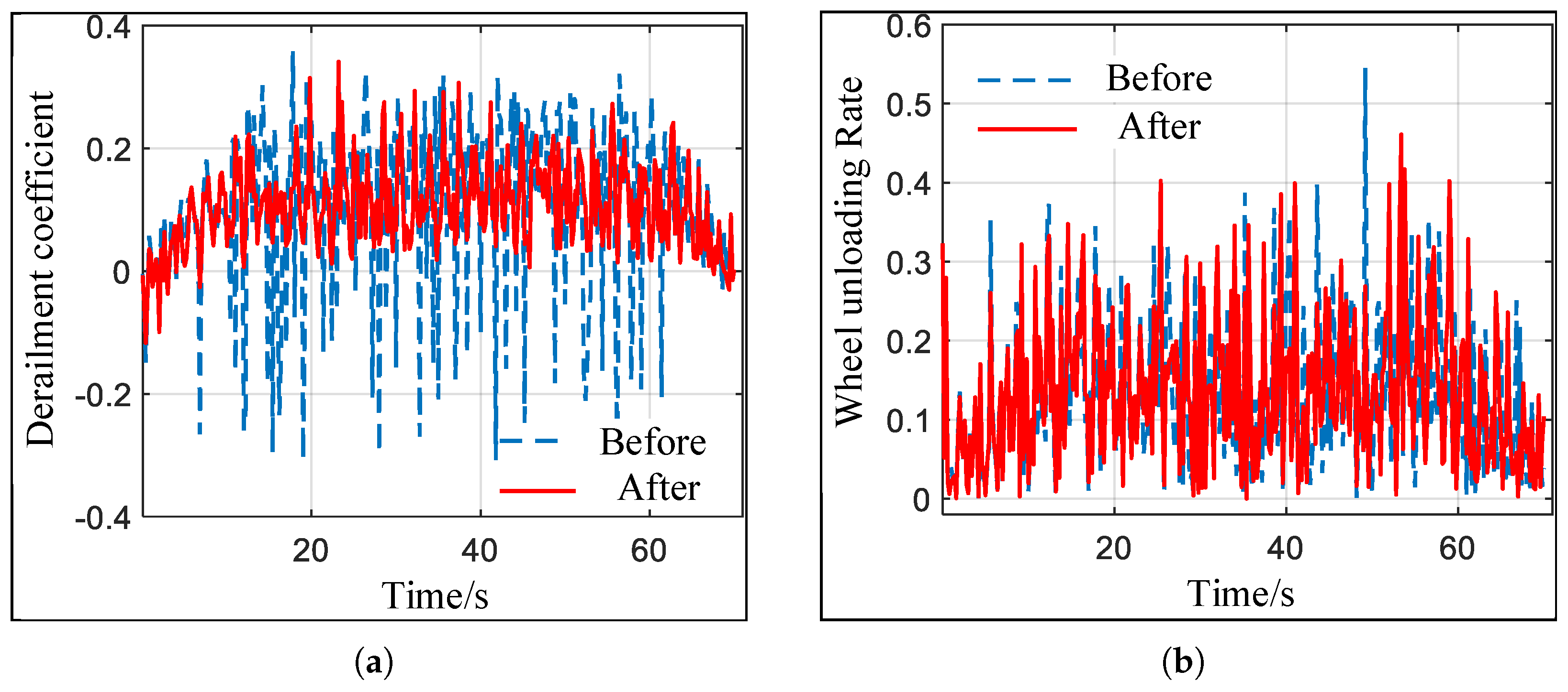
Train curve running safety indicators: wheel–rail vertical force, wheel–axle lateral force, wheel load reduction rate, derailment coefficient. The calculation results are shown in Figure 10 and Figure 11 and Table 5.

Figure 10.
Comparison of train running wheel–rail forces. (a) Wheel–rail vertical force before and after optimization. (b) Axle lateral force before and after optimization.

Figure 11.
Comparison of train running stability. (a) Derailment coefficient before and after optimization. (b) Wheel unloading rate before and after optimization.
Table 5.
Numerical results for the stability of curved running of two types of trains.
As shown in Figure 10, except for a few isolated points, the optimized wheel–rail vertical force has decreased, thereby reducing the impact between the wheel and the rail to some extent. Under the same operating conditions, the optimized profile shows a significant reduction in the wheel–axle lateral force compared to the pre-optimization state. According to the numerical results, the wheel–axle lateral force value has decreased by approximately 4.9% compared to the pre-optimization state. As shown in Figure 11, the derailment coefficient and wheel load reduction rate of the train with the optimized profile have decreased significantly. According to the numerical calculation results in Table 5, the derailment coefficient has decreased by approximately 6.6%, and the wheel load reduction rate has decreased by approximately 4.5%.
4.3. Curving Performance Analysis of the Two Profiles After Long-Term Service
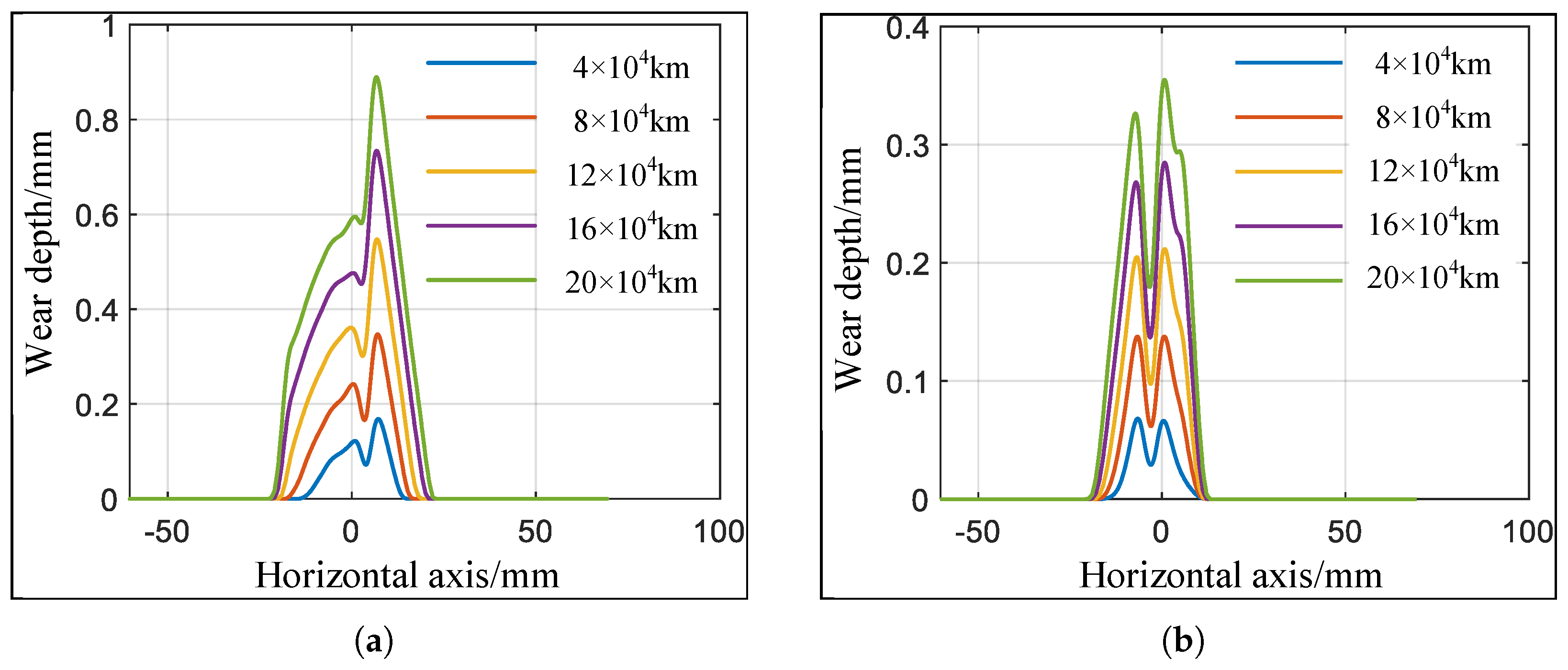
4.3.1. Wear Simulation Analysis Under Two Profile Conditions
The trains were equipped with optimized front and rear profiles for wear simulation analysis. The results are shown in Figure 12 and Figure 13. Figure 12a shows the tread wear depth of the train after running 200,000 km with the initial contour, Figure 12b shows the tread wear depth of the train after running 200,000 km with the optimized contour, and Figure 13 compares the maximum tread wear depth of the optimized front and rear contours.
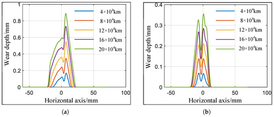
Figure 12.
Optimization of tread wear depth before and after optimization. (a) Tread wear depth before optimization. (b) Tread wear depth after optimization.
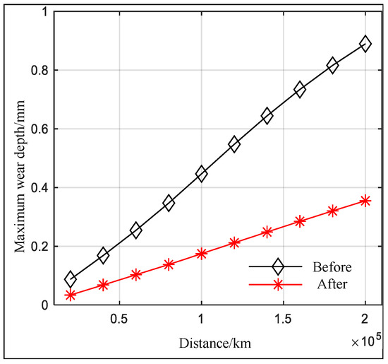
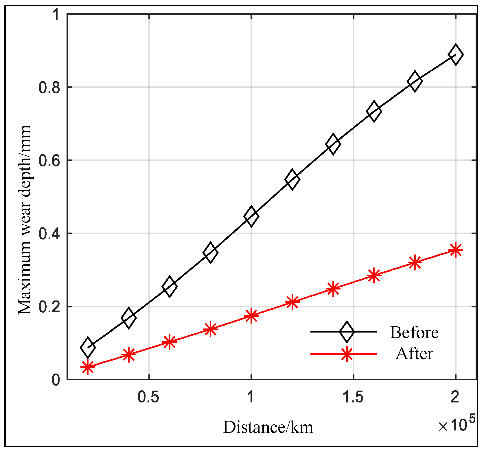
Figure 13.
Comparison of maximum tread wear depth before and after optimization.
As shown in Figure 13, when the train has traveled 200,000 km, the maximum tread wear depth of the pre-optimized profile is 0.889 mm, while that of the post-optimized profile is 0.355 mm. The maximum tread wear depth of the optimized profile has been reduced by 60.1%. The tread wear of train wheels equipped with the optimized profile is less than that of the pre-optimized profile, and as the operating mileage increases, the difference in maximum tread wear depth between the optimized and pre-optimized profiles gradually increases.
4.3.2. Curving Performance Analysis with Two Worn Profiles
Under the same operating conditions as described above, the wear profiles of the original and optimized profiles were compared after 200,000 km of operation. The results are shown in Figure 14 and Figure 15 and Table 6. As shown in Figure 14, the lateral force on the axle of the optimized train has been significantly reduced. According to the numerical calculation results in Table 6, the vertical force between the wheel and rail has decreased by approximately 2.5%, and the lateral force on the axle has decreased by approximately 10.8%.
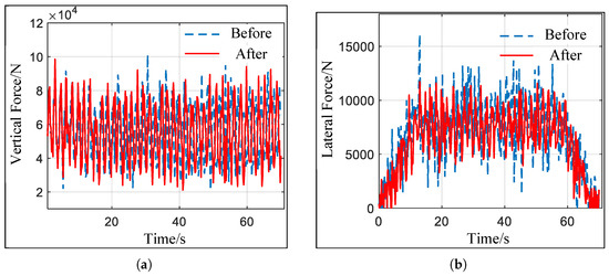
Figure 14.
Comparison of train running wheel–rail forces after wear. (a) Wheel–rail vertical force before and after optimization. (b) Axle lateral force force before and after optimization.

Figure 15.
Comparison of train operation stability after abrasion. (a) Derailment coefficient before and after optimization. (b) Wheel unloading rate before and after optimization.
Table 6.
Numerical results of curve running stability of two types of trains after long-term service.
As can be seen from Figure 15, the derailment coefficient of the optimized train has been significantly reduced. According to the calculation results in Table 6, the derailment coefficient has been reduced by approximately 2.9%, and the wheel load reduction rate has been reduced by approximately 1.6%.
5. Conclusions
This paper proposes a data-driven multi-objective optimization design method for wheel profile. The optimized profile was validated from two aspects: vehicle dynamics characteristics and long-term service performance. The main conclusions are as follows:
- (1)
- A data-driven model is used to establish the mapping relationship between design variables and objective function values. Combined with the established RPSTC-GJO optimization algorithm, the wheel tread profile of the train is optimized, resulting in a tread profile that effectively reduces wheel wear and lateral forces on the axle.
- (2)
- Comparing the wheel–rail wear index and operational smoothness of the optimized and non-optimized profiles on different tracks, the optimized profile demonstrated significant improvements in wheel–rail wear index and train operational smoothness. Additionally, tests were conducted on the train’s curve-passing performance on curved tracks, where the optimization effects on lateral forces on the axle and derailment coefficient were more pronounced, while vertical forces on the wheel–rail interface and wheel load reduction rates also showed varying degrees of improvement.
- (3)
- Comparing the wear volume and curve-passing performance of the optimized and unoptimized profiles after long-term service, the wheel wear prediction results for 200,000 km indicate that the tread wear of the optimized profile has been significantly improved, with the maximum wear depth reduced by 60.1%. Furthermore, the optimized tread exhibits better curve-passing performance after wear simulation.
Author Contributions
Data measurement, M.L., H.D. and B.K.; methodology, M.W. and X.Y.; and funding acquisition, M.W. All authors have read and agreed to the published version of the manuscript.
Funding
This research was funded by the National Natural Science Foundation of China (Grant Nos. 12393783, 52422218 and 12472020), and the Natural Science Foundation of Hebei Province (Grant No. E2024210122).
Institutional Review Board Statement
Not applicable.
Informed Consent Statement
Not applicable.
Data Availability Statement
The raw data supporting the conclusions of this article will be made available by the authors upon request.
Conflicts of Interest
Authors Mao Li, Hao Ding and Bin Kong were employed by the company Guoneng Shuohuang Railway Development Co., Ltd. The remaining authors declare that the research was conducted in the absence of any commercial or financial relationships that could be construed as a potential conflict of interest.
References
- Souza, A.F.D. Influence of the wheel and rail treads profile on the hunting of the vehicles. Trans. ASME 1985, 107, 167–174. [Google Scholar]
- Enblom, R. Deterioration mechanisms in the wheel-rail interface with focus on wear prediction: A literature review. Veh. Syst. Dyn. 2009, 47, 661–700. [Google Scholar] [CrossRef]
- Magel, E.E.; Kalousek, J. The application of contact mechanics to rail profile design and rail grinding. Wear 2002, 253, 308–316. [Google Scholar] [CrossRef]
- Heumann, H. Zur Frage des Radreifen-umrisses. Organ Fortschritte Eisenbahnwesens 1934, 89, 336–342. [Google Scholar]
- Heller, R.; Law, E.H. Optimizing the wheel profile to improve rail vehicle dynamic performance. Veh. Syst. Dyn. 1979, 8, 116–122. [Google Scholar] [CrossRef]
- Shevtsov, I.Y.; Markine, V.L.; Esveld, C. Optimal design of wheel profile for railway vehicles. Wear 2005, 258, 1022–1030. [Google Scholar] [CrossRef]
- Shevtsov, I.Y.; Markine, V.L.; Esveld, C. An inverse shape design method for railway wheel profiles. Struct. Multidiscip. Optim. 2007, 33, 243–253. [Google Scholar]
- Zhang, J.; Wen, Z.; Sun, L.; Jin, X. Wheel profile design based on rail profile expansion method. J. Mech. Eng. 2008, 44, 44–49. [Google Scholar] [CrossRef]
- Zhang, J.; Wang, Y.; Jin, X.; Cui, D. Geometric design method of wheel profile for improving wheel-rail contact condition. J. Traffic Transp. Eng. 2011, 11, 36–42. [Google Scholar]
- Polach, O. Wheel profile design for target conicity and wide tread wear spreading. Wear 2011, 271, 195–202. [Google Scholar] [CrossRef]
- Gerlici, J.; Lack, T. Railway wheel and rail head profiles development based on the geometric characteristics shapes. Wear 2011, 271, 246–258. [Google Scholar] [CrossRef]
- Igesti, M.; Innocenti, A.; Marini, L.; Meli, E.; Rindi, A.; Toni, P. Wheel profile optimization on railway vehicles from the wear viewpoint. Int. J. Non-Linear Mech. 2013, 53, 41–54. [Google Scholar] [CrossRef]
- Rosenbrock, H.H. An automatic method for finding the greatest or least value of a function. Comput. J. 1960, 3, 175–184. [Google Scholar] [CrossRef]
- Mirjalili, S.; Mirjalili, S.M.; Lewis, A. Grey wolf optimizer. Adv. Eng. Softw. 2014, 69, 46–61. [Google Scholar] [CrossRef]
- Persson, I.; Iwnicki, S.D. Optimisation of railway wheel profiles using a genetic algorithm. Veh. Syst. Dyn. 2004, 41, 517–526. [Google Scholar]
- Novales, M.; Orro, A.; Bugarin, M.R. Use of a genetic algorithm to optimize wheel profile geometry. Proc. Inst. Mech. Eng. Part F J. Rail Rapid Transit 2007, 221, 467–476. [Google Scholar] [CrossRef]
- Iwnicki, S.D. The effect of profiles on wheel and rail damage. Int. J. Veh. Struct. Syst. 2009, 1, 99–104. [Google Scholar] [CrossRef]
- Choi, H.-Y.; Lee, D.-H.; Lee, J. Optimization of a railway wheel profile to minimize flange wear and surface fatigue. Wear 2013, 300, 225–233. [Google Scholar] [CrossRef]
- Zeng, W.; Qiu, W.; Ren, T.; Sun, W.; Yang, Y. Multi-objective optimization of rail pre-grinding profile in straight line for high speed railway. J. Shanghai Jiao Tong Univ. (Sci.) 2018, 23, 527–536. [Google Scholar] [CrossRef]
- Cui, D.; Wang, R.; Allen, P.; An, B.; Li, L.; Wen, Z. Multi-objective optimization of electric multiple unit wheel profile from wheel flange wear viewpoint. Struct. Multidiscip. Optim. 2018, 59, 279–289. [Google Scholar] [CrossRef]
- Lin, F.; Zhou, S.; Dong, X.; Xiao, Q.; Zhang, H.; Hu, W.; Ke, L. Design method of LM thin flange wheel profile based on NURBS. Veh. Syst. Dyn. 2021, 59, 17–32. [Google Scholar] [CrossRef]
- Ye, Y.; Qi, Y.; Shi, D.; Sun, Y.; Zhou, Y.; Hecht, M. Rotary-scaling fine-tuning (RSFT) method for optimizing railway wheel profiles and its application to a locomotive. Railw. Eng. Sci. 2020, 28, 160–183. [Google Scholar] [CrossRef]
- Qi, Y.; Dai, H.; Wu, P.; Gan, F.; Ye, Y. RSFT-RBF-PSO: A railway wheel profile optimisation procedure and its application to a metro vehicle. Veh. Syst. Dyn. 2022, 60, 3398–3418. [Google Scholar] [CrossRef]
- Archard, J.F. Contact and rubbing of flat surfaces. J. Appl. Phys. 1953, 24, 981–988. [Google Scholar] [CrossRef]
- Zhao, W.G.; Wang, L.Y.; Zhang, Z.X. A novel atom search optimization for dispersion coefficient estimation in groundwater. Future Gener. Comput. Syst. 2019, 91, 601–610. [Google Scholar] [CrossRef]
- Nitish, C.; Muhammad, A.M. Golden jackal optimization: A novel nature-inspired optimizer for engineering applications. Expert Syst. Appl. 2022, 198, 16924. [Google Scholar] [CrossRef]
- Choi, B.K.; Yoo, W.S.; Lee, C.S. Matrix Representation for NURBS curves and surfaces. Comput.-Aided Des. 1990, 22, 235–240. [Google Scholar] [CrossRef]
- Wang, M.; Wang, Y.; Chen, E.; Liu, Y.; Liu, P. Prediction model of high-speed train tread wear based on identity mapping multi-layer extreme learning machine. J. Mech. 2022, 54, 1720–1731. [Google Scholar]
- International Union of Railways (UIC). UIC 519: Method for Determining the Equivalent Conicity, 1st ed.; International Union of Railways: Paris, France, 2004. [Google Scholar]
- Dong, X.; Wang, Y.; Wang, L.; Zhang, Y. Study on reprofiling strategy for high-speed train wheel treads. China Railw. Sci. 2013, 34, 88–94. [Google Scholar]

Disclaimer/Publisher’s Note: The statements, opinions and data contained in all publications are solely those of the individual author(s) and contributor(s) and not of MDPI and/or the editor(s). MDPI and/or the editor(s) disclaim responsibility for any injury to people or property resulting from any ideas, methods, instructions or products referred to in the content. |
© 2025 by the authors. Licensee MDPI, Basel, Switzerland. This article is an open access article distributed under the terms and conditions of the Creative Commons Attribution (CC BY) license (https://creativecommons.org/licenses/by/4.0/).