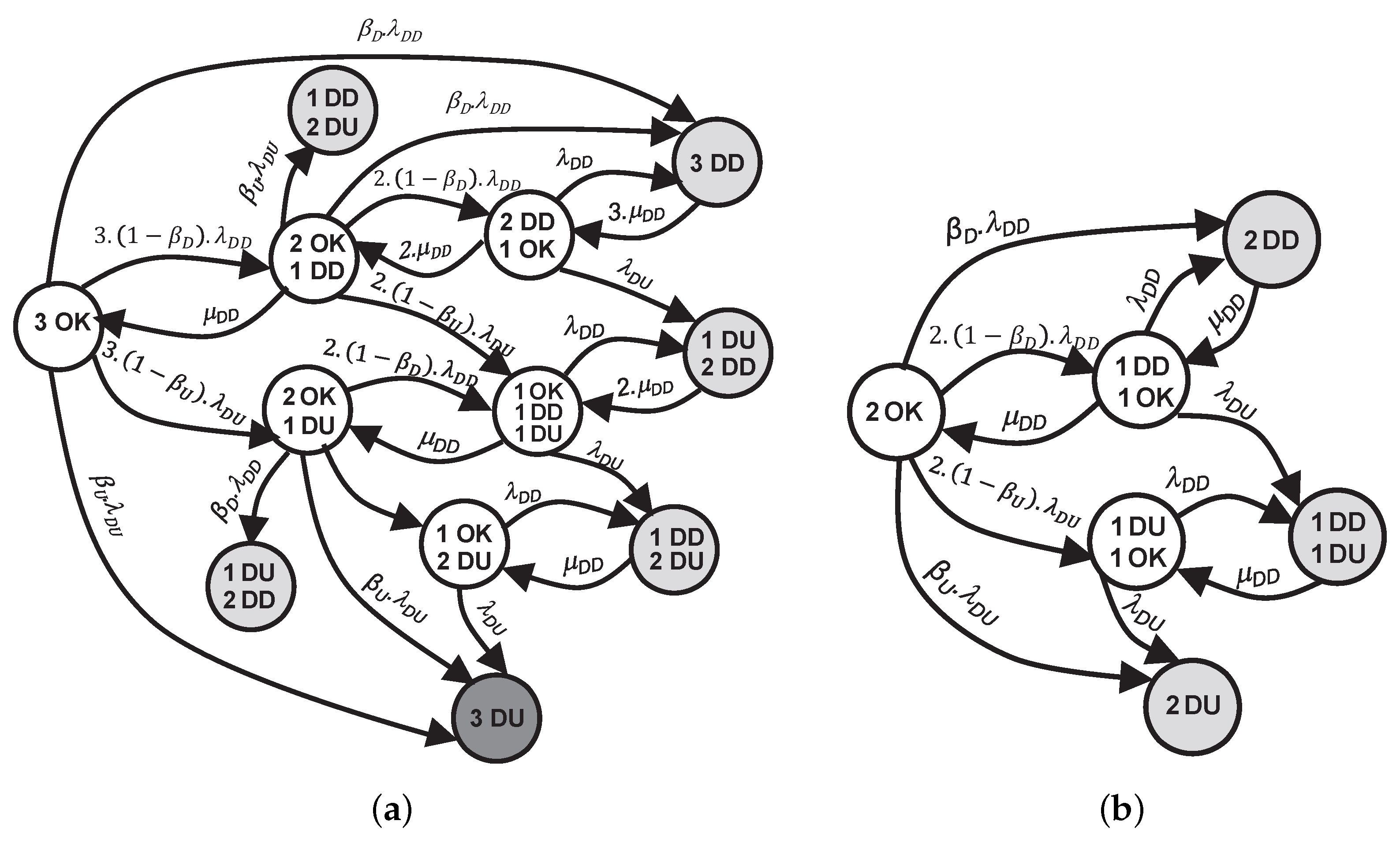
5.1. 1oo3 Structure
This specific architecture, previously introduced and extensively analyzed in the preceding section, led to the formulation of several Conditional Probability Tables (CPTs), as shown in
Table 2,
Table 3,
Table 4,
Table 5 and
Table 6. These CPTs represent the probabilistic dependencies between component states, conditioned on the status of the proof test, and form the core of the dynamic Bayesian network (DBN) model. Based on this foundation, the next step involves implementing the complete probabilistic model illustrated in
Figure 2. This model enables the evaluation of system unavailability by computing the instantaneous PFD at a given time, which subsequently allows for the determination of the average PFD over the mission period (PFD
). These two reliability indicators play a crucial role in evaluating the performance of the architecture and gaining insights into its behavior under demand scenarios.
To illustrate the applicability of the proposed model and assess the effectiveness of the testing strategy, a numerical case study is presented, focusing on a 1oo3 system architecture. Although the analysis focuses on this configuration, this choice is made strictly for illustrative purposes and does not limit the applicability of the approach to the entire SIS. Based on the defined testing strategies, two extreme cases are examined for the actuator layer operating under imperfect proof-testing conditions.
Strategy I: Simultaneous testing, where the three components are tested at the same time during each test cycle of the proof.
Strategy II: The proposed strategy introduced in this study, where only one component is tested during each proof test interval.
A comparative analysis between the two strategies for the 1oo3 structure is presented based on proof test parameters. In our proposed model, the test nodes for each layer serve as exogenous variables, influencing the stochastic process and layer unavailability computation. By simulating the dynamic model, the instantaneous Probability of Failure on Demand for the actuator layer is computed through successive inferences using the Conditional Probability Table provided in
Table 3,
Table 4,
Table 5 and
Table 6.
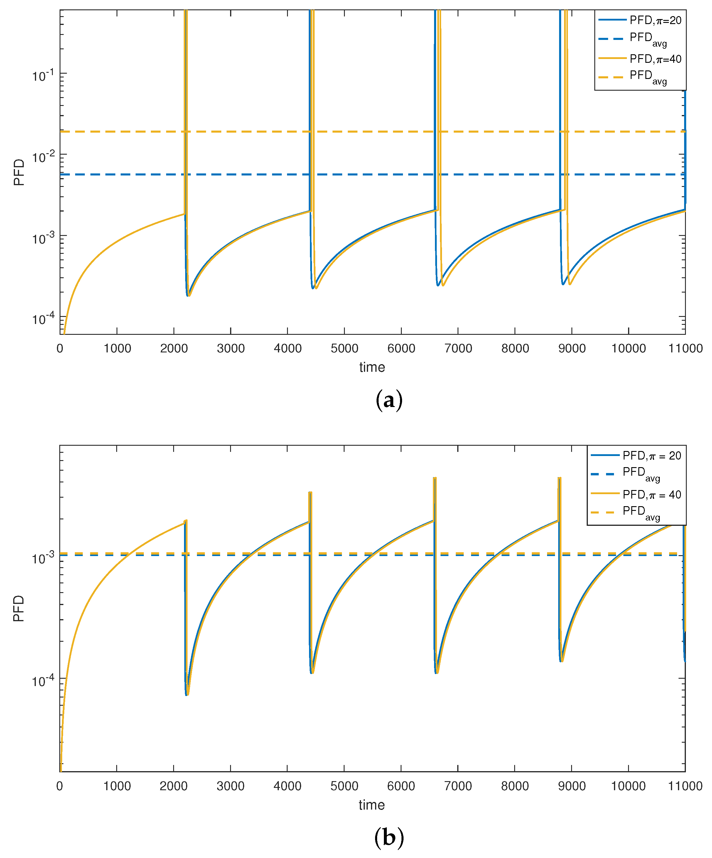
Under Strategy I,
Figure 5a illustrates the variation in the 1oo3 structure unavailability and its average value,
, represented semi-logarithmically for two test durations (20 h and 40 h). Comparing the simulation cases reveals the pronounced impact of
on
variation. As depicted in
Figure 5a, the PFD of the structure increases to 1 for all the test periods, indicating complete unavailability of the 1oo3 architecture throughout the test duration (
) due to simultaneous testing of all the components.
To address complete unavailability, we propose modifying the test strategy for the actuator layer. Strategy II, our proposed alternating test strategy, is then implemented to mitigate the impact of prolonged test durations (
).
Figure 5b demonstrates that Strategy II induces less variation in unavailability compared to the previous case, thanks to non-simultaneous tests. The observed decrease in availability is primarily attributed to the structural change in the actuator layer from a 1oo3 to a 1oo2 configuration. Notably, the variation in the
due to the alternating test strategy is clearly discernible. With
h, the
ranges from 1.0134 ×
(
Figure 5a) to 0.10276 ×
(
Figure 5b).
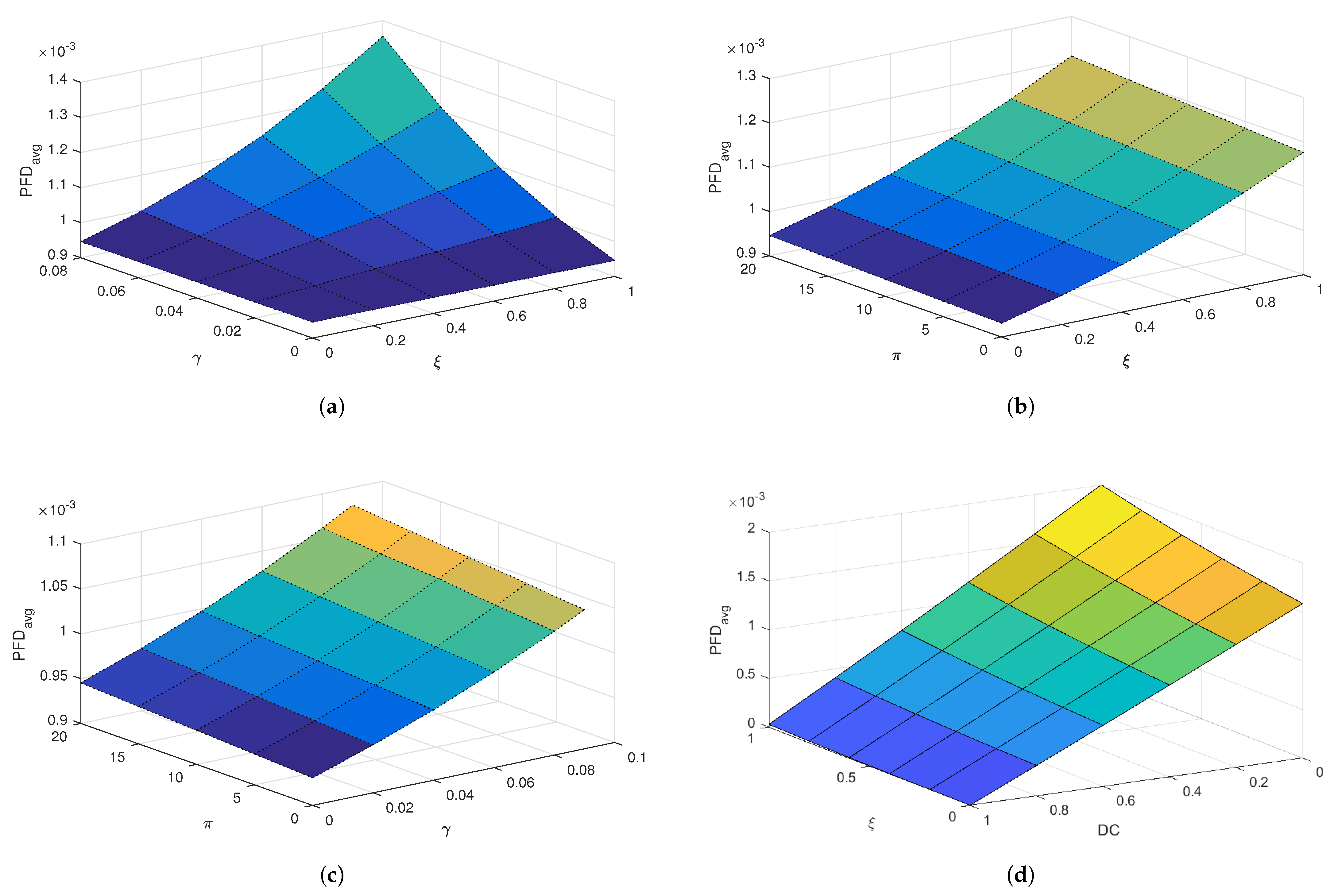
Furthermore, to assess the effectiveness of the proposed alternating proof test strategy, a detailed sensitivity analysis was carried out. This analysis explores the influence of critical parameters related to both proof and diagnostic testing on the PFD for the actuator layer, which is modeled using a dynamic Bayesian network (DBN) approach.
The parameters under consideration include
,
,
, and the rate
. These variables are known to play a significant role in shaping the unavailability profile of safety instrumented components. In this analysis, four distinct scenarios were investigated. In each case, two of the parameters mentioned above were varied simultaneously, while the remaining two were kept constant. This approach enables a comprehensive evaluation of the joint impact of the variable parameters on the PFD
and thus on the overall reliability of the system. The simulation results are illustrated using 3D surface plots, as shown in
Figure 6.
The first case, illustrated in
Figure 6a, presents the variation in the PFDavg as a function of
and
. The results indicate that increasing either
or
leads to a noticeable rise in the PFDavg. This shows that proof tests that are both ineffective and prone to causing failures significantly degrade system reliability.
Figure 6b illustrates the second case, in which the influence of
and
on the PFD
is examined. The results demonstrate that ineffective tests allow for latent faults to persist, while longer testing periods increase the exposure to unavailability. The alternating test strategy proposed in this study mitigates these effects by avoiding simultaneous testing of all redundant components, thereby preserving partial functionality during test intervals.
Figure 6c illustrates the third case, which investigates the combined influence of
and
, with
and
held constant. The results reveal that both parameters contribute to an increase in system unavailability, and their combined impact becomes more significant as
increases. The alternating test strategy helps reduce the adverse impact of extended test durations on the PFD
. In this final case depicted in
Figure 6d, the relationship between
and
is examined. The PFD
increases with higher test ineffectiveness, while it decreases with improved diagnostic coverage. This result illustrates the compensatory role of diagnostics: even if the proof test is suboptimal, a robust diagnostic system can detect failures during normal operation, significantly enhancing reliability.
The results of the sensitivity analysis emphasize the effectiveness of the proposed alternating testing strategy to reduce the negative impact of imperfect and prolonged testing on system availability. This strategy allows for alternating tests, where only one component of a layer is tested at a time rather than testing all the components simultaneously. The integration of this strategy into the maintenance planning of safety instrumented systems is therefore recommended, especially in configurations with extended proof test durations.
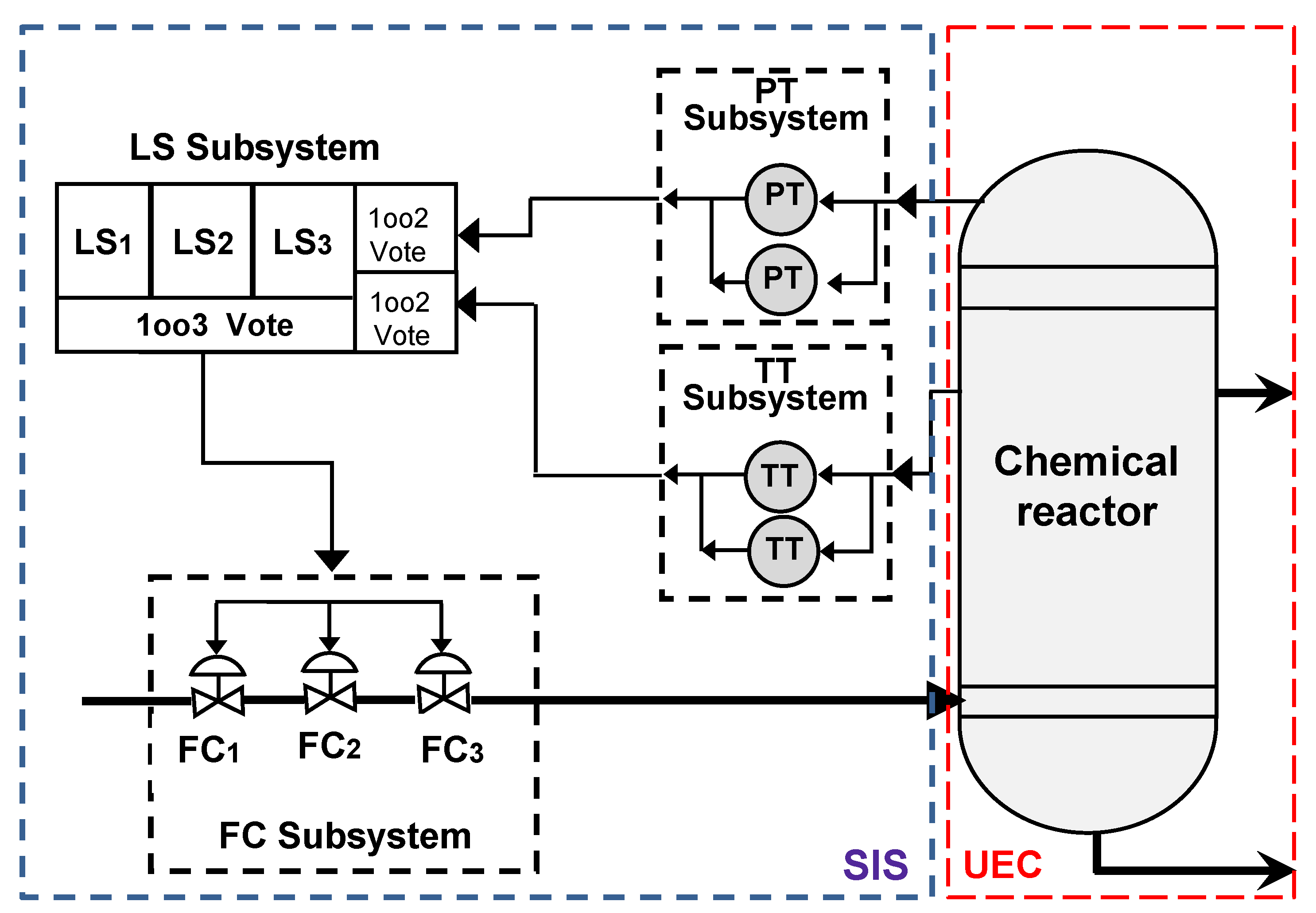
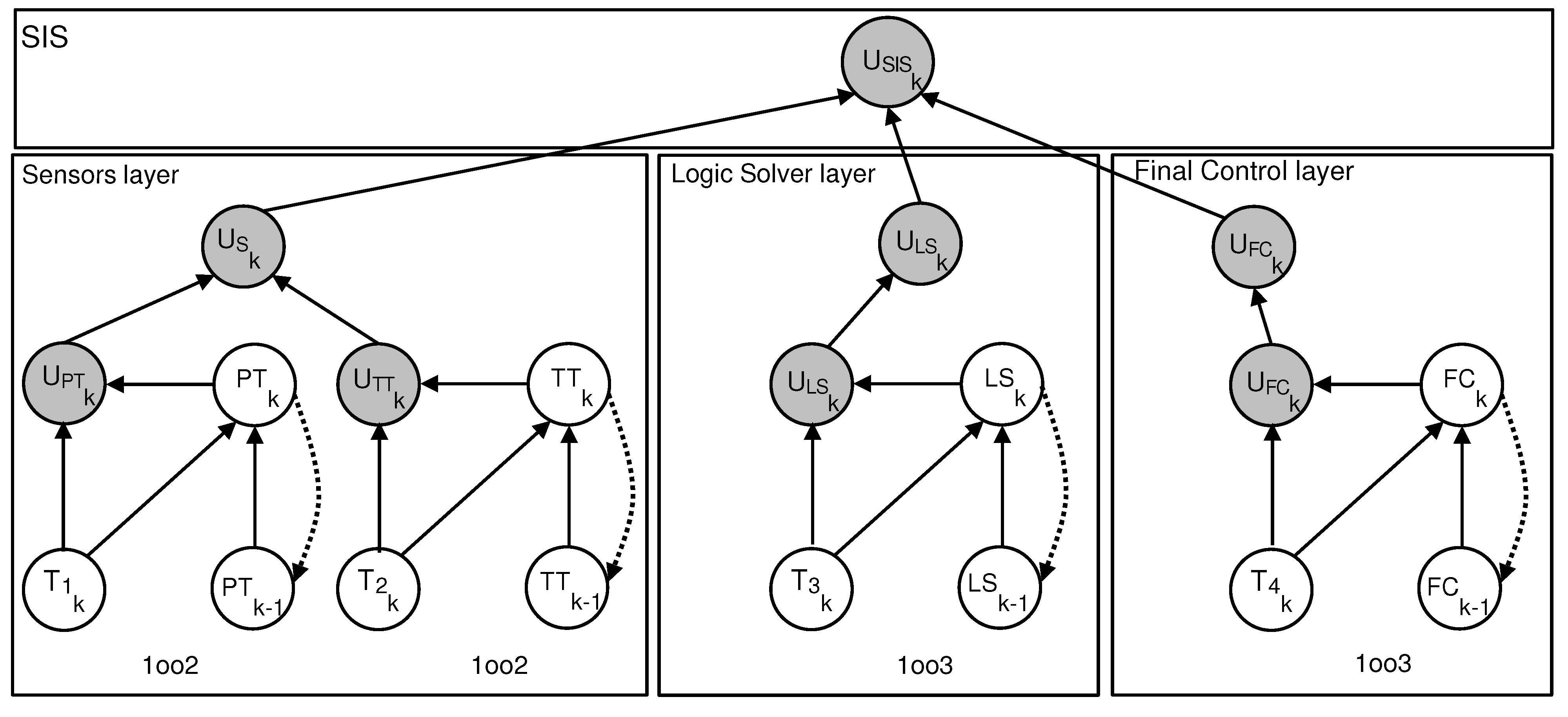
5.2. Overview of the Entire SIS
The considered SIS is organized into three distinct layers. The sensor layer includes two blocks, each composed of two sensors, temperature transmitters (TTs) and pressure transmitters (PTs), arranged in parallel. The Logic Solver (LS) layer operates in a 1oo3 configuration, whose behavior has already been described in the previous section. Finally, the actuator layer, comprising the final control elements, also follows a 1oo3 architecture.
Figure 7 illustrates the functional architecture of the SIS studied, which is organized into three distinct and independent layers. Each layer or subsystem can be individually modeled using a DBN, as depicted in the reference model of
Figure 2.
The global functionality of the SIS is captured through a combination of these layer-specific models, arranged in a serial/parallel configuration. This structure enables the estimation of the overall unavailability of the system (that is, PFD), based on the unavailability of each layer, which is modeled using a configuration .
The construction of the equivalent DBN model of the entire SIS involves defining the CPTs that determine the state of each layer based on the states of its components and the status of the proof-testing process. In particular, the adopted alternating test strategy assumes that, during each test cycle, only one component per layer is subjected to verification, which introduces temporal dynamics into the unavailability of the entire SIS.
The structure of each layer is represented by a dedicated node within the DBN, and the corresponding CPT can be derived with relative ease. The DBN model described in
Figure 7 constitutes the equivalent probabilistic representation of the entire SIS studied. This structure is systematically derived from the functional graph depicted in
Figure 2, which models the logical dependencies and dynamic interactions between the various operational layers.
The numerical data of the key parameters that characterize the components of each functional layer, together with those related to the proof-testing strategies, are summarized in
Table 7. These values are then used to compute the overall PFD
of the SIS by combining the average PFDs of the individual layers, while accounting for their mutual interactions.
The parameter numerical values presented in
Table 7 were selected based on commonly cited sources in the literature on safety instrumented systems (SISs), particularly concerning performance evaluation under proof-testing policies (e.g., [
27,
28]). These values fall within realistic ranges observed in engineering practice and are frequently employed in numerical studies to support the validation and benchmarking of reliability modeling approaches. The aim is to illustrate the methodological applicability of the proposed strategy rather than to replicate a specific case.


