Abstract
To enhance the reliability of unmanned hydro-mechanical transmission tractors, a fault diagnosis method for their power-shift system was developed. First, fault types were identified, and sample data was collected via a test bench. Next, a feature extraction method for data dimensionality reduction and a deep learning network called W_SCBAM were introduced for fault diagnosis. Both W_SCBAM and conventional algorithms were trained 20 times, and their performance was compared. Further testing of W_SCBAM was conducted in various application scenarios. The results indicate that the feature extraction method reduces the sample length from 46 to 3. The fault diagnosis accuracy of W_SCBAM for the radial-inlet clutch system has an expectation of 98.5% and a variance of 1.6%, respectively, outperforming other algorithms. W_SCBAM also excels in diagnosing faults in the axial-inlet clutch system, achieving 97.6% accuracy even with environmental noise. Unlike traditional methods, this study integrates the update of a dimensionality reduction matrix into network parameter training, achieving high-precision classification with minimal input data and lightweight network structure, ensuring reliable data transmission and real-time fault diagnosis of unmanned tractors.
1. Introduction
Tractors are the most important agricultural power machinery, supplying power for essential tasks like plowing, sowing, spraying, and harvesting. With the global population rising, the demand for food has increased, while the agricultural workforce has shrunk. Consequently, research on unmanned tractors [1,2] has gained significant attention, leading to the emergence of unmanned farms in China. These tractors often use power-shift transmissions [3,4] or multi-range hydro-mechanical transmissions (HMTs) [5,6,7] for automatic shifting, both relying on power-shift technology with wet clutches as key components. For instance, Figure 1 illustrates the unmanned HMT tractor we are developing with Shandong Weifang Luzhong Tractor Co., Ltd. in Weifang, China. The HMT power-shift system is a complex mechanical, electrical, and hydraulic system. Malfunctions during autonomous operation can be hard to detect and address, affecting the tractor’s shifting quality, reducing clutch lifespan, delaying agricultural work, and compromising safety. Thus, there is an urgent need to develop automatic fault diagnosis systems for unmanned tractors to enhance their operational reliability.
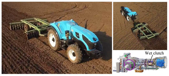
Figure 1.
Unmanned HMT tractor developed by research team.
Current methods for identifying transmission faults include manual diagnosis, model-based diagnosis, machine learning-based diagnosis, and deep learning-based diagnosis. Manual diagnosis is notably inaccurate and inefficient. Model-based diagnosis uses the residual between mathematical models and physical systems as a diagnostic basis [8,9], but constructing accurate models for complex systems is challenging. Machine learning-based diagnosis involves creating a classifier to map data sample features to machine health status. For instance, Lupea et al. [10] utilized support vector machines (SVM) with cubic kernels for diagnosing helical gear faults, while Afia et al. [11] compared the effectiveness of Random Forests (RFs), Ensemble Trees (ETs), and Nearest Neighbors (KNNs) in diagnosing transmission faults. This method does not require understanding fault mechanisms but relies heavily on the quality of selected features. Deep learning, which constructs classifiers through multi-layer neural networks, automatically extracts features from large datasets, offering higher accuracy and adaptability. Common deep learning networks for transmission fault diagnosis include the Convolutional Neural Network (CNN), Recurrent Neural Network (RNN), and Deep Belief Network (DBN). CNNs, often used for 2D data, can also process 1D time series data, as seen in Dutta et al.’s [12] lightweight 1D CNN for fault diagnosis. Some studies transform time series data into 2D images to leverage CNNs, as described in Vashishtha et al.’s [13] research. Long Short-term Memory (LSTM) and its variants are the most commonly used RNNs for transmission fault diagnosis. There is substantial research in this area. For instance, Cao et al. [14] simulated the transmission’s operating state using real spindle speed on a test bench and proposed a deep bi-directional LSTM network to classify vibration signals under various faults. Yin et al. [15] enhanced the precision and generalization of transmission fault diagnosis by optimizing the LSTM network with cosine loss. Similar studies include those by Ravikumar et al. [16] and An et al. [17]. Compared to CNN, LSTM is primarily used for processing time series data with long-term dependencies. In recent years, there has been a trend towards integrating CNN and LSTM for fault diagnosis in complex systems. For instance, Kang et al. [18] utilized the CNN-LSTM algorithm to improve the extraction of local features from time series signals, achieving fault classification of transmission vibration signals in complex operating environments. However, CNN-LSTM models often have numerous training parameters, leading to longer training times. DBN is another classic transmission fault diagnosis algorithm, but it also faces similar issues. It has multiple training parameters and is prone to overfitting with limited sample data or complex models. Relevant research includes the work of Andhale and Parey [19], as well as Zhao et al. [20].
The fault diagnosis research discussed focuses primarily on traditional mechanical transmissions, particularly their key components like gears and bearings. Research on diagnosing faults in HMT transmissions is still in its early stages. The primary source of faults in this transmission type is the wet clutch and its hydraulic control circuit. Wang et al. [21], one of the authors of this study, initially explored this issue using kernel methods in 2014. Over the past decade, subsequent research has continued, but due to limited dataset sizes, traditional machine learning methods [22,23,24] have been predominantly used. In 2023, Wang et al. [25] enhanced the Echo State Network (ESN) and introduced deep learning to this field. The time series signals analyzed in these studies primarily involve clutch pressure during shift, which can be captured using low-cost pressure sensors. However, applying these methods to real tractors presents challenges. Clutch pressure data is typically collected by the transmission control unit (TCU), which has limited computing power. Therefore, the TCU must send clutch pressure data to the onboard computer, where fault diagnosis algorithms are deployed, via the CAN bus. The commonly used CAN protocols in vehicles are the standard low-speed CAN 2.0 and high-speed CAN FD, with CAN FD being backward compatible with CAN 2.0. Tractor manufacturers typically produce tractors with varying power and complexity in small batches, and the production of high-end tractors is much lower. Bulk purchasing TCUs based on standard CAN bus has a cost advantage. Based on these considerations, we view the standard CAN bus as a hardware limitation for fault diagnosis research, aiming to develop a cost-effective and widely compatible classification algorithm. However, the pressure data length used for fault diagnosis in the aforementioned studies ranges from 64 to 300, and transmitting this data with 16-bit accuracy would require 128 to 600 bytes, while the standard CAN bus can only transmit 8 bytes of data at a time. This not only jeopardizes data transmission reliability but also increases the risk of CAN bus congestion. Additionally, the power-shift time of HMT tractors is very short, necessitating real-time performance in fault diagnosis. Given that existing fault diagnosis methods for power-shift systems typically require extensive data input and complex classification algorithms, they are not well-suited for practical applications. To address these issues, our objective is to achieve high-precision, high-robustness fault diagnosis of tractor power-shift systems with minimal sample length and a lightweight network structure.
This paper is structured as follows: Section 1 introduces classic transmission fault diagnosis algorithms and highlights the challenges in diagnosing faults in tractor power-shift systems. Section 2 covers the collection of sample data, feature extraction methods, and the fault diagnosis algorithms used. Section 3 analyzes the fault diagnosis results and tests their reliability across different tractor power-shift systems. Section 4 summarizes the study’s conclusions and outlines future research directions.
2. Methods and Materials
2.1. Test Bench
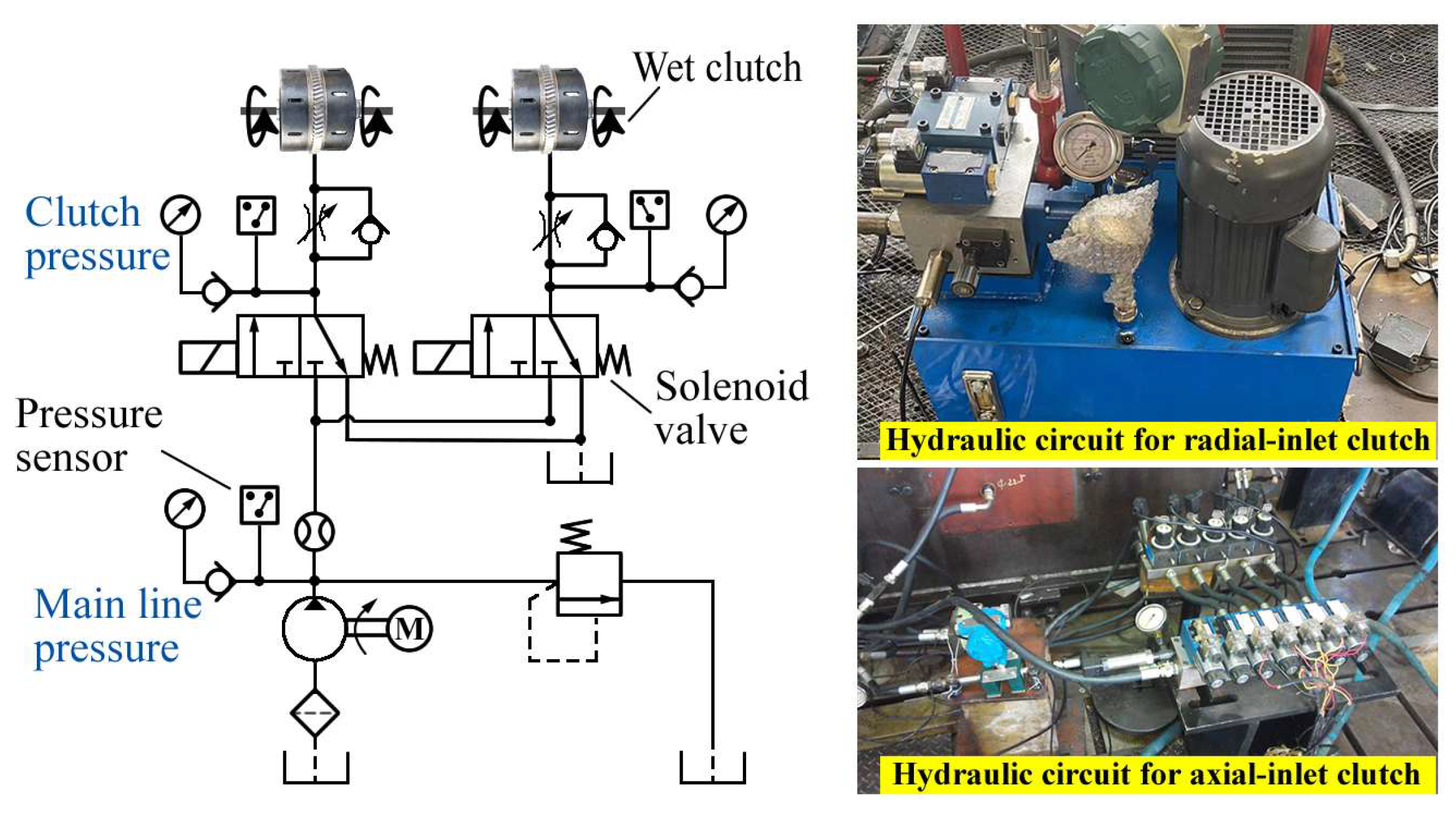
The power-shift system in tractor HMT differs from traditional power-shift transmissions. Most can achieve speed synchronization before shifting, allowing solenoid directional valves or step current-controlled proportional pressure reducing valves to directly drive the wet clutch for range switching. The HMT power-shift system typically features a hydraulic oil circuit as depicted in Figure 2. When the solenoid valve is activated, pressure oil enters the clutch cylinder, pushing the piston to press the driving and driven friction plates, engaging the clutch. When the solenoid valve is deactivated, the piston resets under the return spring, separating the clutch. Two common types of wet clutches are the radial-inlet and axial-inlet clutches. Due to structural and performance differences, separate test benches were built for each to gather fault data. The equipment details for these test benches are provided in Table 1 and Table 2, respectively.

Figure 2.
Hydraulic circuit of tractor power-shift system.

Table 1.
Equipment utilized in the hydraulic test bench for the radial-inlet clutch.
Table 2.
Equipment utilized in the hydraulic test bench for the axial-inlet clutch.
2.2. Mechanism of Pressure Formation
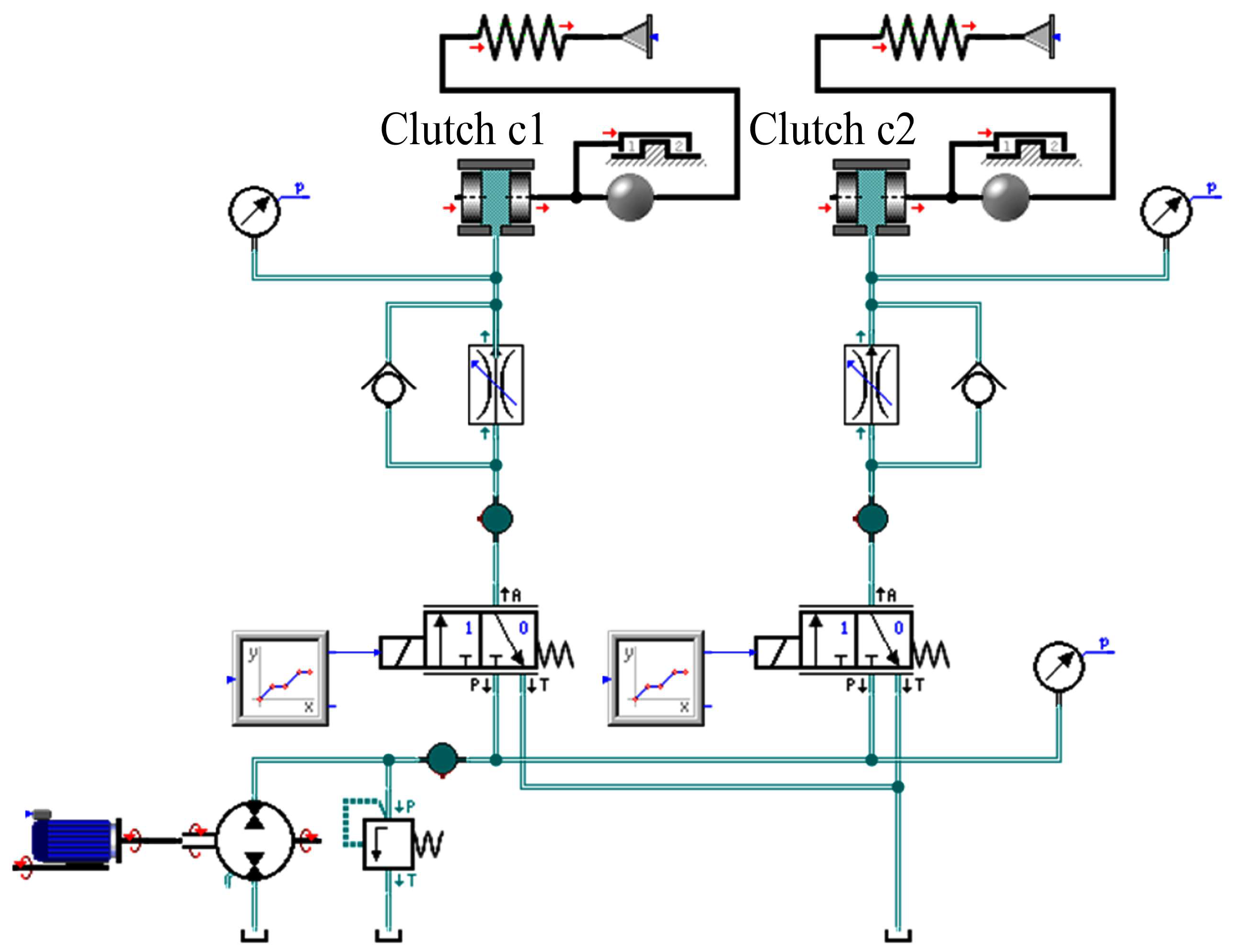
In our initial study, we utilized flow data for diagnosing faults in the power-shift system. However, measuring pressure in hydraulic systems is more cost-effective and quicker. To gain a better understanding of the pressure formation process during shifting, we developed a dynamic model of the power-shift system using SimulationX (Version 3.5), as illustrated in Figure 3. This model accounts for factors like frictional forces during clutch piston movement and the structure of the clutch end stop.
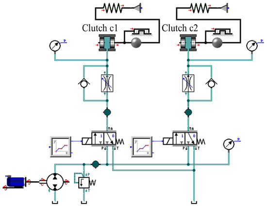
Figure 3.
Simulation model of power-shift system.
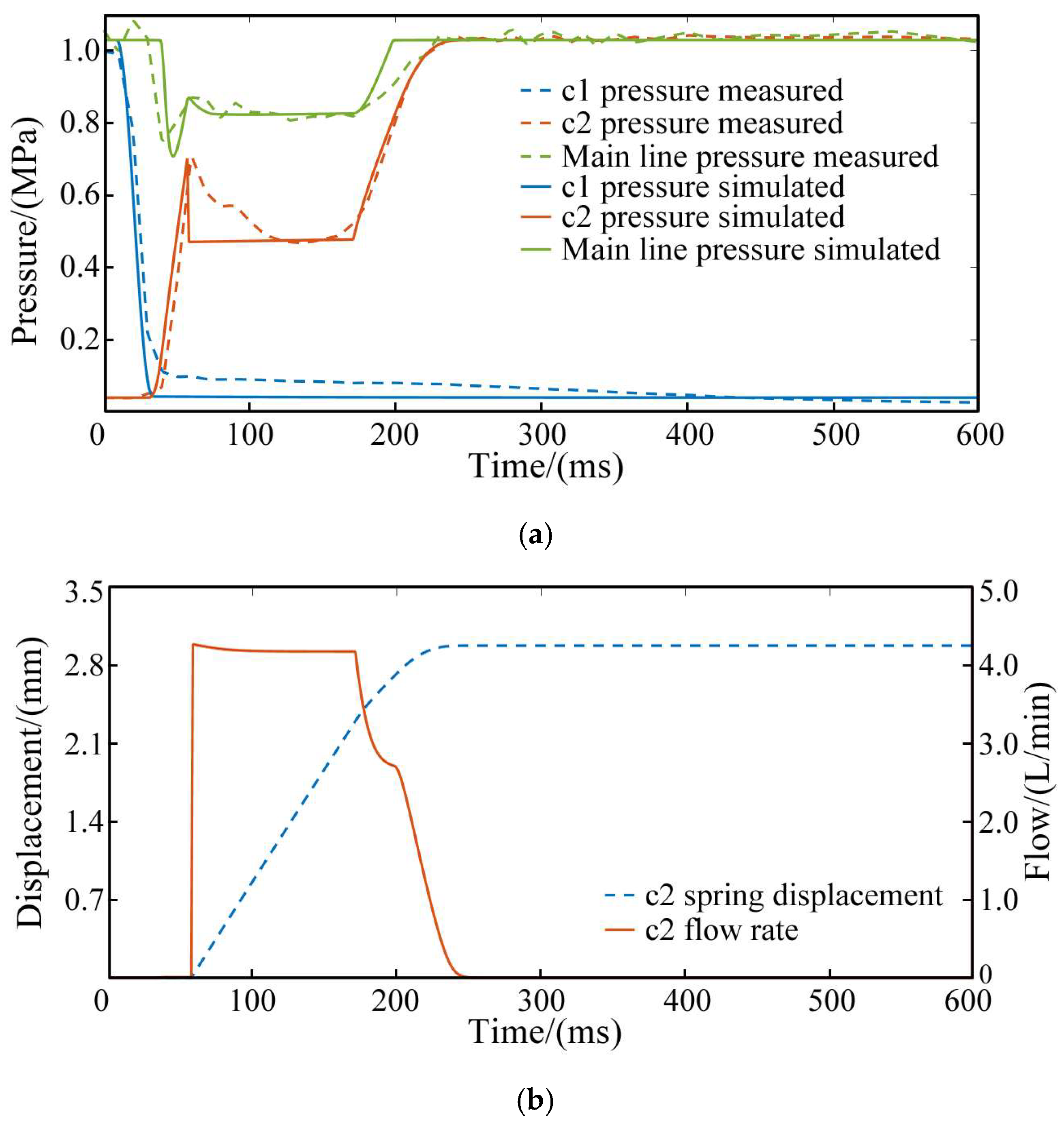
The experimental verification and simulation results of the model during shifting are shown in Figure 4. Figure 4a demonstrates that the simulation results for the pressure of clutch c1 to be separated, clutch c2 to be engaged, and the main line pressure align closely with the experimental results, confirming the model’s reliability. Figure 4b provides simulation data that is difficult for sensors to capture, specifically the displacement of the return spring and the instantaneous flow rate of the engaged clutch.

Figure 4.
Results obtained from experiments and simulations. (a) Oil pressure. (b) Spring displacement and clutch flow rate.
The following is shown in the figure:
(1) For clutch c1, the pressure drops quickly once shifting begins, as the solenoid valve spool’s movement connects the clutch oil circuit to the tank.
(2) For clutch c2, the pressure rises in three stages to its final value. In the first stage, hydraulic oil flows into the clutch cylinder after the solenoid valve is energized. The pressure quickly increases until it overcomes the spring reaction force and the static friction force of the piston, causing the clutch piston to move. In the second stage, the piston begins to close the gap between the friction plates. Since the sliding friction is less than the static friction, the clutch pressure decreases after the piston starts moving. In the later part of this stage, as the return spring compresses, the oil pressure slightly increases to counter the growing spring resistance. The clutch pressure level and duration during this phase depend on the combined forces of spring reaction and sliding friction from the piston movement. In the third stage, the piston reaches the end stop, and the clutch pressure quickly rises to the final value. Due to the elasticity of the end stop, the piston displacement increases slightly to fully close the gap between the friction plates, completing the clutch’s power engagement. This is why the clutch flow rate does not immediately drop to zero.
(3) The main line pressure remains unaffected by clutch c1. Once the solenoid valve is energized, the main line connects to the oil circuit of clutch c2, causing the main line pressure to fluctuate with the clutch engagement pressure. The hydraulic pump continuously supplies flow, ensuring the main line pressure stays at or above the clutch pressure, resulting in pressure loss between the main line and the clutch oil circuit.
Based on the analysis, it is clear that the clutch separation pressure does not influence the main line pressure. The rapid pressure drop during clutch separation makes it challenging to gather sufficient fault information. Consequently, this study proposes a fault diagnosis solution for the clutch engagement phase. The scheme uses only the main line pressure and clutch pressure, which are interrelated in their formation, as inputs for the deep learning model. Many hydraulic system failures alter the shape of the oil pressure curve, with different failures affecting the oil pressure at various stages. This forms the theoretical basis for subsequent feature extraction through dimensionality reduction.
2.3. Dataset Construction
2.3.1. Fault Classification
Before developing diagnostic algorithms, it is essential to first identify the various types of faults. In addition to the normal mode F0, common faults in the oil circuit of radial-inlet clutches include oil channel leakage (F1), oil circuit blockage (F2), solenoid valve spool jamming (F3), and clutch piston jamming (F4). For axial-inlet clutches, which require rotary joints, the sealing ring at this joint is prone to damage. Therefore, in diagnosing faults in power-shift systems using these clutches, sealing ring damage replaces the less frequent failure rate mode F3 and is labeled as fault F3′.
For fault F1, we installed a throttle valve in parallel with the oil pipe connected to the clutch. Increasing the valve opening can cause varying degrees of oil channel leakage. For fault F2, we placed a speed control valve in series on the oil pipe connected to the clutch, simulating different levels of oil circuit blockage by reducing the valve opening. For fault F3, we replaced the return spring of the solenoid valve with a stacked gasket and kept the solenoid valve energized, preventing the spool from moving. Different gasket thicknesses simulate the spool being jammed at various positions. For fault F4, we filled the external clearance of the piston with sandpaper when the clutch engaged, preventing it from resetting and simulating a jam. For fault F3′, we replaced the normal sealing ring with a damaged one to simulate this fault.
This research will initially focus on developing a fault diagnosis algorithm for a power-shift system that incorporates a radial-inlet clutch.
2.3.2. Data Acquisition
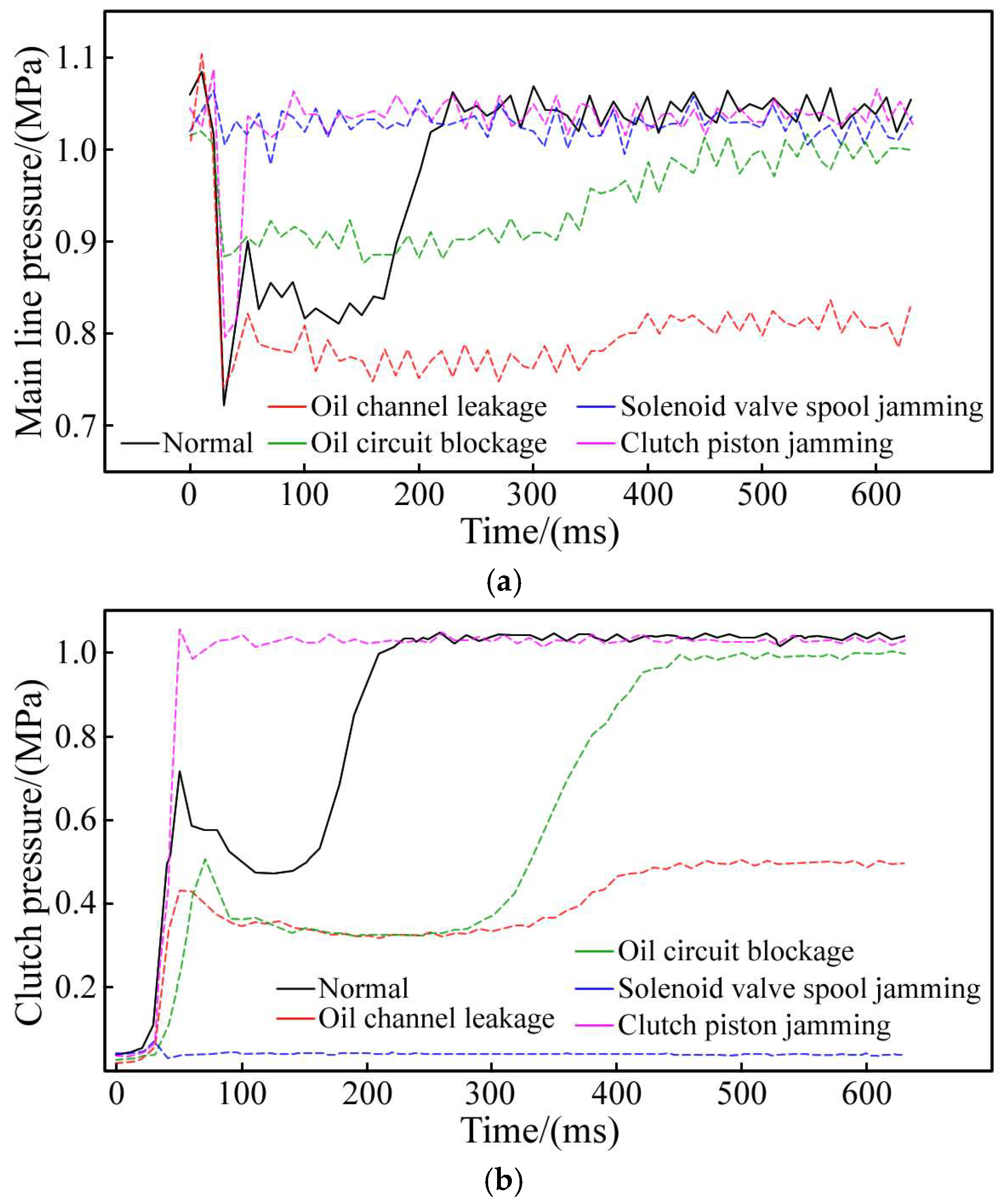
The experiment utilized two sets of Labview programs and two NI USB-6009 data acquisition cards to manage the solenoid valve and gather pressure data. To facilitate data segmentation, a handshake signal was sent from the control card to the measurement card via a signal line when the solenoid valve’s state changed. The Labview program simultaneously read and displayed both the handshake and pressure signals, which were then recorded in a spreadsheet. All pressure sensors were calibrated prior to testing. Given the experiment’s extended duration, the oil temperature would gradually increase, impacting the hydraulic oil’s viscosity. However, we have not imposed any restrictions on these environmental conditions to ensure the dataset encompasses data from these complex working scenarios. The partial fault pressure data obtained from the test bench is shown in Figure 5. This figure indicates that the fault’s impact spans all three stages of the clutch engagement process. Note that the shape of the pressure curve is related to the severity of the fault, and only the most typical fault pressure curve is shown in the figure. We obtained over 30,000 fault samples on the test bench, and randomly selected 15,000 samples for algorithm research, including 3000 in the normal group and 3000 in each of the four fault groups.
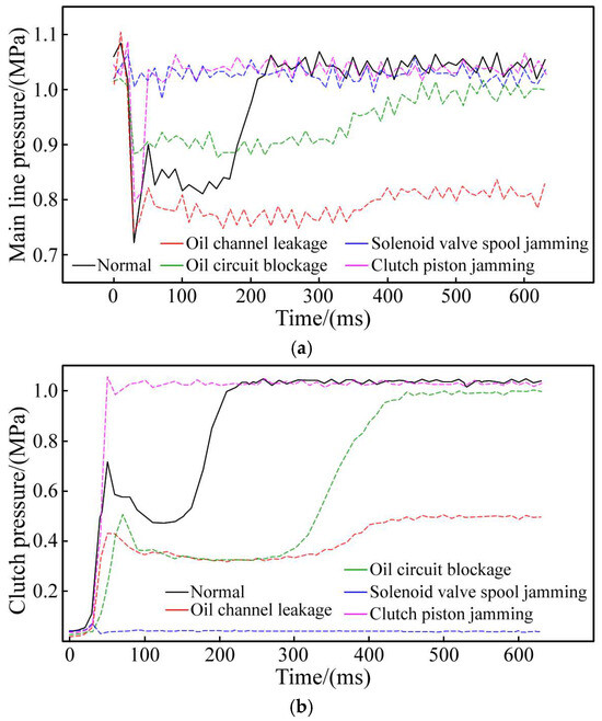
Figure 5.
Clutch pressure in fault mode. (a) Main line pressure. (b) Clutch pressure.
By analyzing the normal pressure curve from the experiment, the clutch pressure reaches 90% of its final value within 220 ms. Given the 10 ms data collection interval, we set the initial number of data points for each sample, including the zero point, to 23. We then concatenate the main line pressure sequence and the clutch pressure sequence into a new sample:
where represents the group of samples in the sample set, with each sample having two channels, and each channel containing 23 features; represents the channel for the main line pressure; represents the channel for the clutch pressure.
2.4. Fault Diagnosis
2.4.1. Feature Extraction
Before discussing the algorithm, we input all 46 data points and 23 randomly selected data points from the sample into the same neural network (adding zeros to the latter to ensure the same number of features). We obtain nearly identical classification results, indicating that not all data in the sample contribute to fault diagnosis. Therefore, we propose a feature extraction method using neural networks to reduce sample length. The idea of this method is to left-multiply the original training set by a dimensionality reduction matrix before inputting it into the neural network. The dimensionality reduction matrix is randomly initialized and iterated along with the neural network. Once training is complete, the dimensionality reduction matrix is adjusted to an appropriate value. This matrix retains the key information of the original training set and can be used to restore the neural network’s attention ranking to the original features. The detailed process is as follows:
By left-multiplying the training set with feature length by the dimensionality reduction matrix , a new training set with feature length can be obtained:
where represents the number of training samples input to the neural network; and represent the length of the input sample and the length of the reduced sample, respectively.
The output of the neural network for the training set is as follows:
The matrix obtained after training serves as a linear transformation that enhances the classification performance of the neural network on the training set . Note that matrix is not unique and varies based on the specific neural network structure.
The significance of each component in the input sample’s feature vector can be assessed by the absolute value of the cosine distance between each base vector in the original sample space and the matrix . Specifically, for the given unit matrix , let represent the space spanned by with its dimension .
can be considered a hyperplane with the dimension of in the space , using the matrix’s rows as the base vector. represents the coordinate of the training set in the space , and represents the coordinates of in the hyperplane .
The normal vector of hyperplane in space , denoted as , is any non-zero solution to the following equation:
Calculate the absolute value of the cosine distance between each basis vector in and the normal vector to create a list A:
where represents the length of the normal vector .
Select the indices of the top largest elements in to form a feature-indexed list . Note that the different number of iterations and randomly initialized hyperparameters in each training process result in different dimensionality reduction matrices and feature-indexed lists being calculated each time. Based on this, extract the features of each sample in the training set according to the calculated list . Denote the sample as and concatenate all samples to obtain a new training set , which is used to train the neural network . The above process can be represented by the following equations:
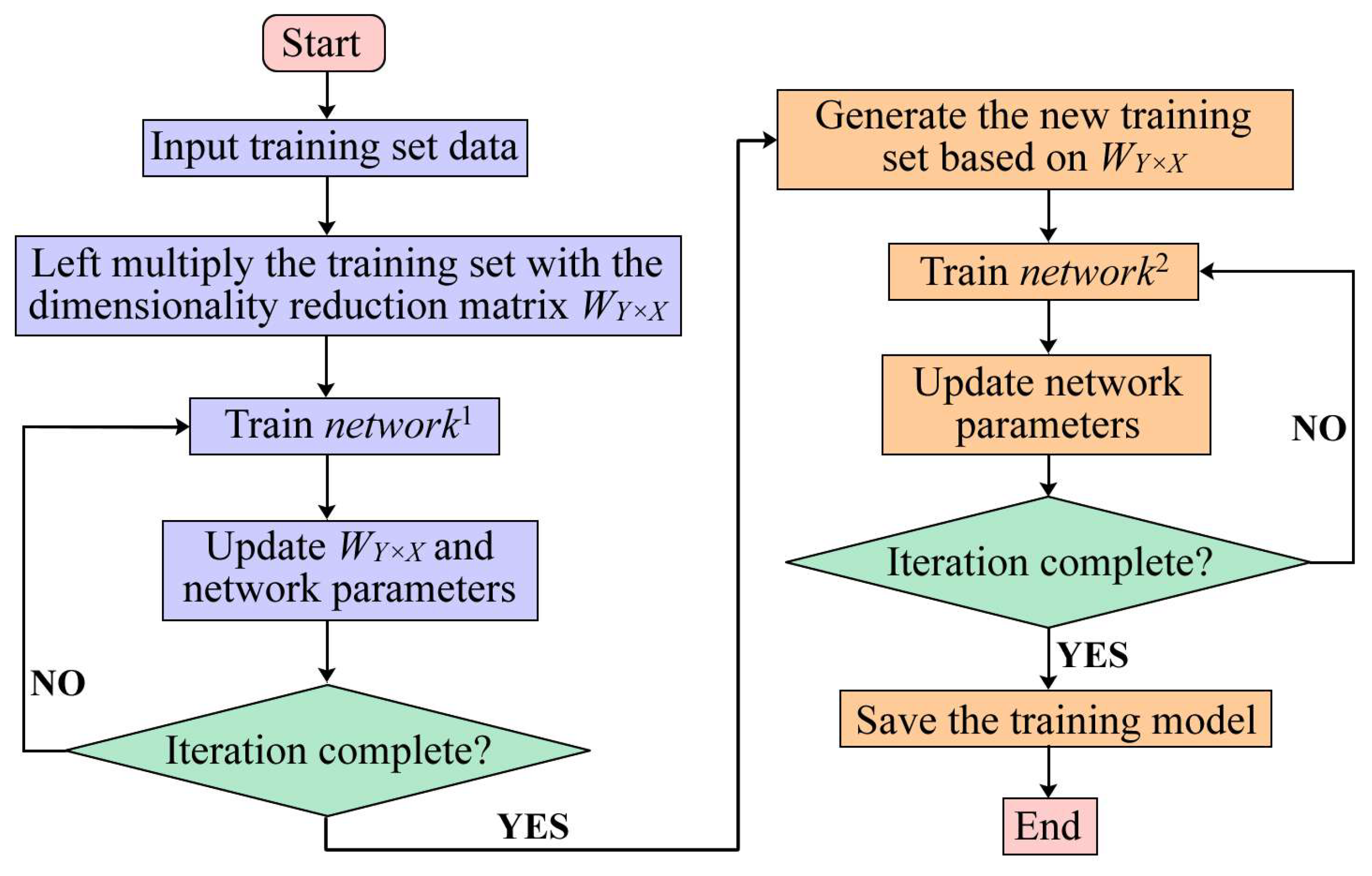
The algorithm described in this article is illustrated in Figure 6. The figure indicates that the algorithm comprises a feature extraction network and a fault diagnosis network . The initial training phase aims to generate the feature index list of for the subsequent training, ultimately resulting in the final fault diagnosis model after the second training phase.
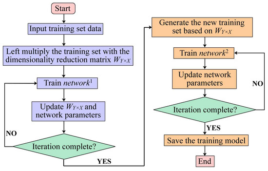
Figure 6.
Flowchart of the fault diagnosis algorithm.
2.4.2. Network Structure
To ensure the feature-indexed list derived from performs well in training, it is specified that the feature extraction network has the same structure as the training network , as illustrated in Figure 7.
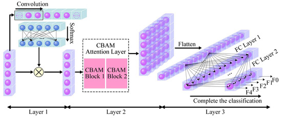
Figure 7.
Neural network structure.
The neural network described consists of three layers:
(1) The first layer: spatial attention layer.
The first layer of applies one-dimensional convolution and nonlinear transformation to the output from Equation (2) along the feature direction. It then calculates the attention assigned by to each feature point of using the function. By dot-multiplying the calculated attention with the original input, the with attention allocation is output. This process can be represented by the following equations:
where represents the convolution kernel of size 3; represents dot multiplication operation.
The first layer adjusts the dimensionality reduction matrix to an appropriate spatial position by assigning varying attention to the features of . During backpropagation, shifts towards positions that allocate high attention and moves away from features with minimal impact on classification. Features that contribute less to fault diagnosis are continuously eliminated, optimizing . Additionally, applying the function along the feature direction ensures the sum of attention weights assigned by the neural network to each feature is equal to 1, intensifying the competition between features.
(2) The second layer: Convolutional Block Attention Module (CBAM) layer.
Convolution enables neural networks to have a larger receptive field in the feature dimension and increases the feature space by learning various convolution kernels. To ensure focuses on significant feature connections for fault diagnosis during backpropagation, and to enable it to concentrate on various sample organization forms (i.e., different channels) during the learning, a 3-sized convolution kernel is used to perform one-dimensional convolution operations on in the feature dimension. The output, processed by the function, is then passed to the next module:
To enable to focus on various spatial features of across different channels or within the same channel during iteration, the plane spanned by , trained by , must reflect more valuable oil pressure data for the neural network. Thus, the CBAM attention mechanism is added after convolution. Unlike other common attention mechanisms like Squeeze-and-Excitation (SE), CBAM incorporates both channel and spatial attention modules, enhancing the model’s performance comprehensively [26]. The corresponding operations can be expressed as follows:
where represents the channel attention operation and represents the spatial attention operation.
In this study, the CBAM attention module was applied only at the one-dimensional level—a special case of its use. Equations (13)–(15) outline the fundamental CBAM calculation module. Two consecutive CBAM modules, referred to as CBAM Block 1 and CBAM Block 2, constitute a complete convolutional attention layer.
(3) The third layer: output layer.
The output from the second layer is first flattened along the feature dimension, then passed through two fully connected layers (FC Layer 1 and FC Layer 2). The final result of the neural network is produced by FC Layer 2:
where represents the linear transformation operation.
Table 3 displays the number of channels and features in each layer of the network structure. We initialize the neural network parameters using standard normal distribution random initialization. The Adam optimizer is used for network optimization with the following hyperparameters: learning rate ; exponential decay rate for the first moment estimate ; exponential decay rate for the second moment estimate ; numerical stability constant . The training process is set to conclude after 200 iterations.
Table 3.
The number of channels and features in each layer of the network.
2.4.3. Multi-Channel Case
The algorithm initially addresses the case where the channel is 1 (i.e., ). For multi-channel training sets (i.e., the training set is ), Equation (2) should be applied to each channel individually. Once neural network training is complete, extract the dimensionality reduction matrix for each channel and apply Equations (5) and (6) to each matrix separately. Based on the feature-indexed lists obtained for each channel, extract the training set to obtain the for each channel. When constructing the neural network, create separate spatial attention layers for each channel. After completing the forward propagation of the first layer in each channel, concatenate the channels along the feature dimension, converting the input data for subsequent layers into single-channel data.
2.4.4. Evaluation Method
The study’s development environment is Python 3.10, and the neural network framework is PyTorch 2.0.1. The 15,000 experimental data sets are divided into training and testing sets at an 8:2 ratio. This results in a training set of 12,000 samples, with 2400 samples per type, and a testing set of 3000 samples, with 600 samples per type.
The proposed algorithm is evaluated using four metrics: Precision, Recall, F1 score, and Accuracy. Their expressions are as follows:
We also use the cross-entropy loss function to measure the difference between the actual output probability distribution and the model’s predicted output probability distribution:
where represents the probability that the model predicts a sample to belong to category .
2.4.5. Algorithms for Comparison
For ease of reference, the algorithm proposed in this study is called W_SCBAM. Here represents the dimensionality reduction matrix, represents the spatial attention mechanism used in the first layer of the neural network, and CBAM represents the one-dimensional CBAM convolutional attention mechanism used in the second layer.
To assess the performance of feature extraction algorithms within the same neural network structure, we compared the classical PCA algorithm with the one proposed in this study. If a matrix can be found for the training set to make a diagonal matrix, then is the eigenvalue matrix:
Combine the top bases with the highest eigenvalues of into a new matrix to replace the dimensionality reduction matrix , and name this algorithm PCA_SCBAM.
To assess the compatibility between the feature extraction algorithm and the neural network, the following methods are used for comparison with the algorithm in this study: replacing the W_SCBAM neural network with a three-layer standard CNN and MLP, respectively, denoted as W_CNN and W_MLP, or removing the first layer of the W_SCBAM neural network, denoted as W_CBAM.
3. Results and Discussion
3.1. Results of Fault Diagnosis
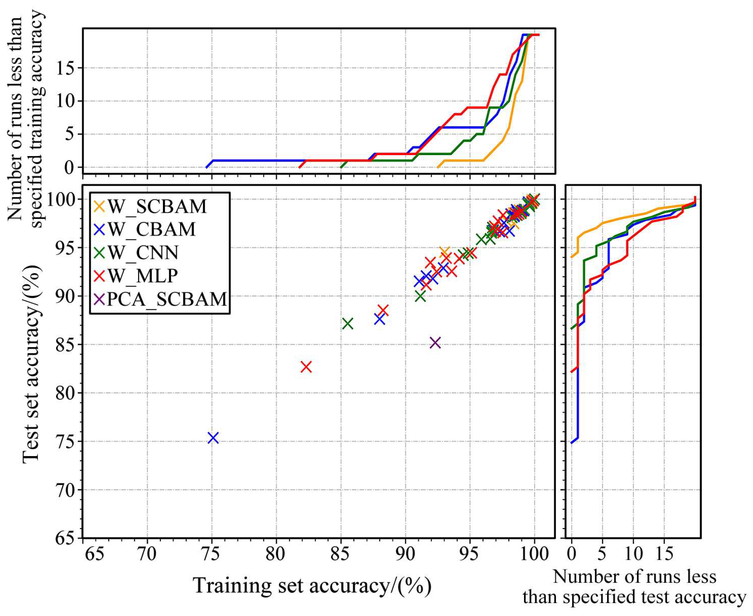
The study’s sample set is dual-channel, making W_SCBAM suitable for multi-channel situations. Preliminary tests show the algorithm can reduce the sample length to three within the allowed accuracy, with two features from the main line pressure channel and one from the clutch pressure channel. Consequently, all comparison algorithms, including W_SCBAM, undergo 20 training repetitions with three sample features to evaluate their effectiveness and robustness. The results are presented in Figure 8. The upper sub-figure indicates the number of times each algorithm’s classification accuracy on the training set falls below the specified value after 20 training sessions, while the right sub-figure shows the same for the test set. Note that the PCA_CBAM algorithm requires only one training session, so its single result is not marked in the sub-figures.

Figure 8.
Results of 20 consecutive training sessions for each algorithm.
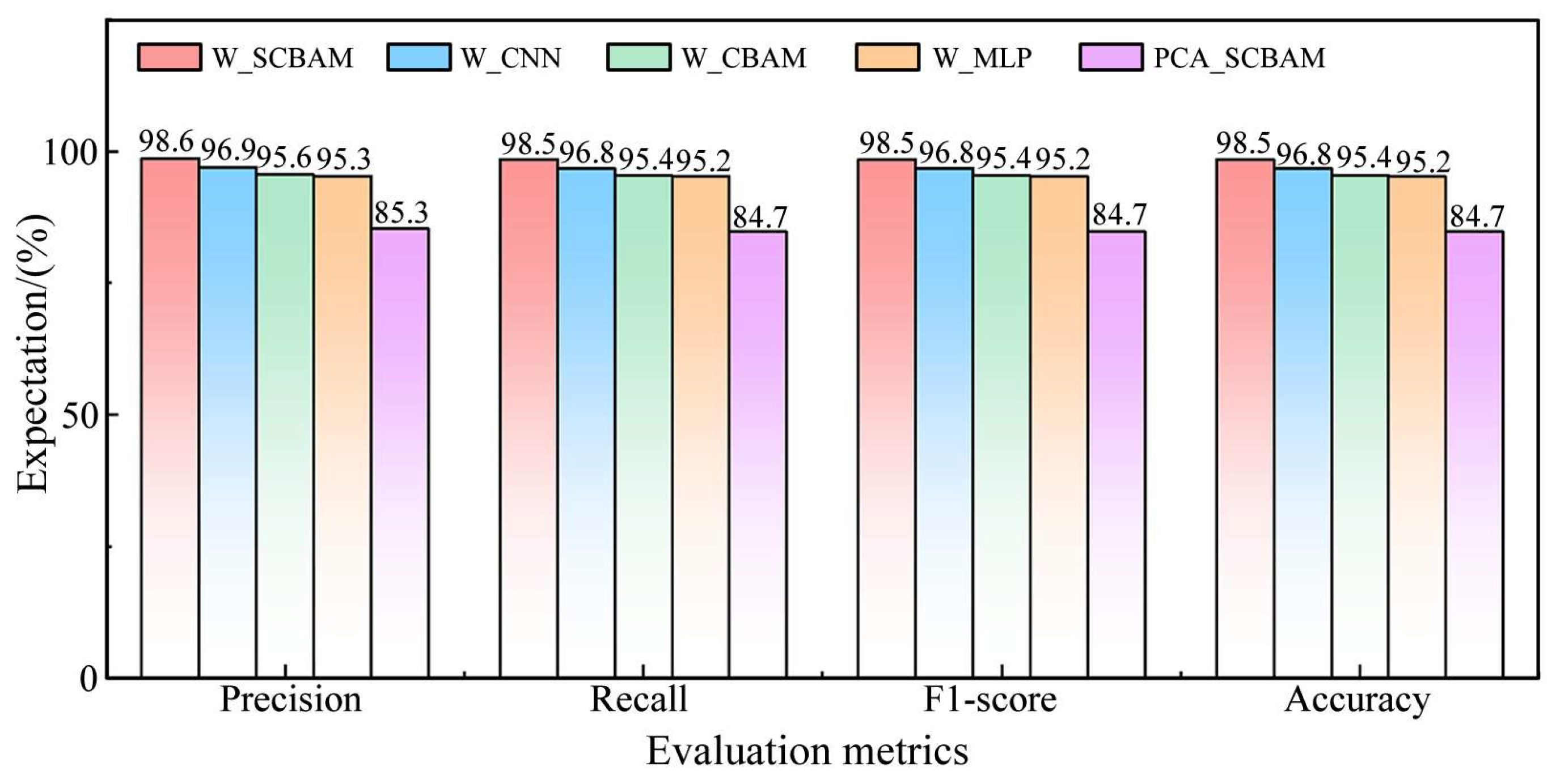
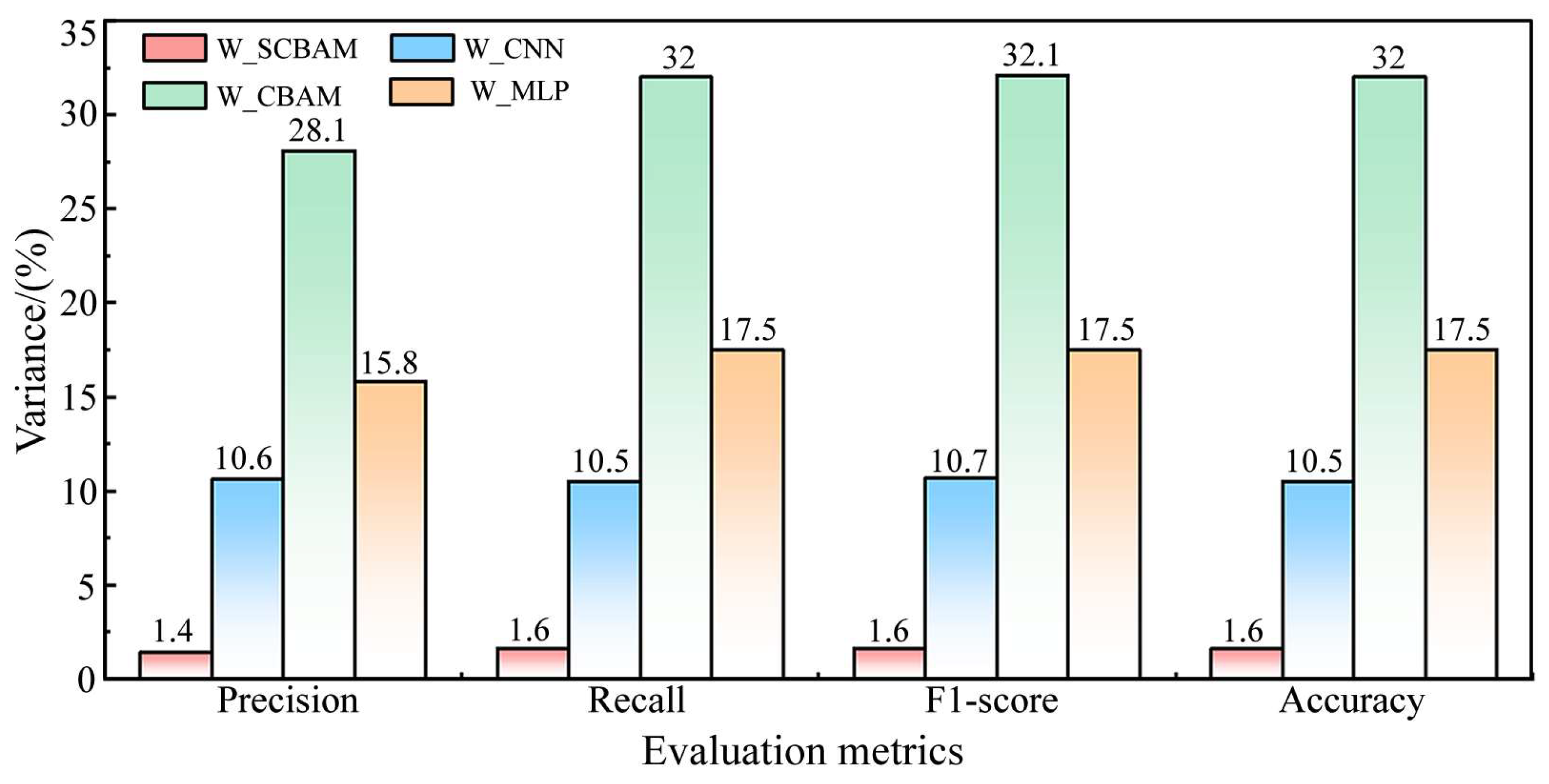
Additional statistics were performed to determine the expectation and variance of each indicator of the algorithm over 20 consecutive tests, as illustrated in Figure 9 and Figure 10, respectively.
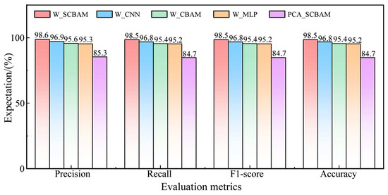
Figure 9.
Expectations of evaluation metrics for each algorithm.
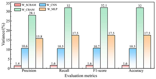
Figure 10.
Variance of evaluation metrics for each algorithm.
(1) Comparison of PCA_SCBAM with other algorithms. Figure 8 indicates that the PCA_SCBAM algorithm achieves 84.7% accuracy in the test set, whereas other algorithms attain at least one solution with over 98% accuracy. Figure 9 demonstrates that the expectations of all metrics for PCA_SCBAM are significantly lower than those of other algorithms in the test set. This suggests that pre-training the dimensionality reduction matrix using neural networks and extracting the feature-indexed list is a valuable approach.
(2) Comparison between W_SCBAM and W_CBAM, W_CNN, W_MLP. Figure 8 indicates that the accuracy of all solutions from W_SCBAM in the test set exceeds 94%, while the proportion of solutions from W_CBAM, W_CNN, and W_MLP that surpass 94% is 70%, 80%, and 55%, respectively. Figure 9 shows that the expectations of the accuracy of W_SCBAM in the test set is higher than W_CBAM, W_CNN, and W_MLP by 3.1%, 1.7%, and 3.3%, respectively. Figure 10 demonstrates that the variance of all evaluation indicators for W_SCBAM is significantly lower than other algorithms in the test set. These results indicate that W_SCBAM has high performance and stability. Additionally, while the neural networks of W_CBAM and W_SCBAM differ only in the first layer, their fault diagnosis performance varies greatly, suggesting that the first layer of the neural network in W_SCBAM significantly impacts feature extraction and fault diagnosis.
(3) Overfitting problem. Figure 8 demonstrates that all algorithm solutions, except for PCA_SCBAM, can be approximated by a proportional function, where test set accuracy equals training set accuracy. This suggests that, even when the sample length is reduced from 46 to 3, these algorithms do not exhibit overfitting issues.
3.2. Test Results Under Different Datasets
To assess the adaptability of W_SCBAM, we conducted fault diagnosis tests in a power-shift system featuring an axial-inlet clutch. Unlike radial-inlet clutches, which can be tested independently, axial-inlet clutches must be tested alongside the transmission shaft and rotary joint. This setup increases the risk of damage to expensive HMT transmissions when introducing artificial faults. To safeguard the transmission, we limited the number of tests and collected 1620 sets of sample data, including environmental noise. We split the samples into a training set and test set in an 8:2 ratio, using a feature-indexed list length of three. We then trained the neural network following the process outlined in Figure 6, with the results presented in Figure 11.
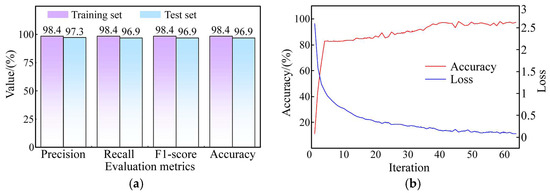
Figure 11.
Fault diagnosis of the power-shift system with an axial-inlet clutch. (a) Fault diagnosis results. (b) Training process of neural networks.
The test results indicate that the proposed W_SCBAM algorithm performs excellently even in noisy environments, achieving an accuracy of 96.9%. Additionally, the algorithm successfully reduced the sample length from 128 to 3, further demonstrating its strong feature extraction capabilities.
Similar to the radial-inlet clutch dataset, an algorithm performance analysis was conducted after 20 consecutive tests, with results presented in Table 4. The accuracy ranged from 96.7% to 98.8%, averaging 97.6%. These results further confirm the algorithm’s robustness and indicate that its accuracy meets application requirements.
Table 4.
Statistical analysis of algorithm performance following 20 consecutive tests.
3.3. Analysis of Algorithm Complexity
The W_SCBAM neural network has only 706 parameters, with forward propagation FLOPS at just 908. We tested it using 5000 randomly generated data sets on an Intel® Core™ i5-11320H processor. The average running time per sample was seconds. Thus, W_SCBAM is an algorithm with few parameters, low computational complexity, and high computational efficiency.
4. Conclusions
This study examined the fault diagnosis of the power-shift system in HMT tractors, yielding the following key findings and conclusions:
(1) By monitoring the main line pressure and clutch pressure of the HMT tractor during shifting, the health of the power-shift system can be effectively assessed. Compared to previous research, this study revealed that most pressure data points do not aid in fault diagnosis. By reducing the data length from 46 to 3, a fault diagnosis accuracy of 98.5% was still achieved, indicating that the data transmitted from the TCU to the CAN bus for fault diagnosis can be significantly minimized.
(2) A new feature extraction algorithm, more effective than traditional PCA, has been introduced. Building on this, a deep learning algorithm called W_SCBAM was developed for diagnosing faults in tractor power-shift systems. Compared to algorithms like PCA_SCBAM, W_CBAM, W_CNN, and W_MLP, W_SCBAM demonstrates higher classification accuracy and stability.
(3) Reducing the sample length from 46 to 3 is an extreme test to validate the algorithm’s performance. In this scenario, the accuracy of W_SCMAM ranges from 94% to 100% across 20 training sessions, fully meeting the application requirements. To further reduce the accuracy fluctuation and enhance the algorithm’s robustness, the sample length can be appropriately increased.
(4) W_SCBAM is effective for power-shift systems featuring both radial-inlet and axial-inlet clutches, demonstrating strong adaptability across various applications. Moreover, the algorithm is resilient to environmental noise and holds significant potential for use in HMT tractors.
The proposed feature extraction method and W_SCBAM network are suitable for power-shift and HMT tractors that change gears (or speed ranges) using wet clutches. The hydraulic and mechanical systems of the wet clutch operate independently, ensuring that the tractor’s load and working environment do not affect oil pressure, thus maintaining the fault diagnosis algorithm’s effectiveness. However, variations in oil pressure curves among wet clutches of different specifications make it challenging to directly apply the trained W_SCMAM across different products. Fortunately, the consistent working principle of wet clutches means that W_SCMAM can be retrained for new clutch models without structural modifications. This study trained the same W_SCMAM model on two clutches with distinct mechanical structures, both achieving excellent diagnostic performance, validating the above perspective. Transfer learning might also be effective, but its feasibility requires further investigation, which is outside the scope of this study.
W_SCBAM is a fault diagnosis algorithm created for unmanned HMT tractors by our research team. Since this concept tractor has not yet been mass-produced, our research data is sourced from a test bench, which is not yet reflective of real-world conditions. In future work, W_SCBAM will be implemented in the unmanned tractor depicted in Figure 1, and its effectiveness and robustness will be evaluated using real fault data and actual operating scenarios.
Author Contributions
Conceptualization, G.W.; methodology, Y.L. (Ya Li) and K.L.; software, Y.L. (Ya Li), K.L. and X.C.; validation, K.Z.; formal analysis, Y.L. (Ya Li) and K.L.; investigation, X.C., K.Z. and Y.L. (Yangting Liu); resources, G.W.; data curation, X.C. and Y.Z.; writing—original draft preparation, Y.L. (Ya Li), K.L., X.C. and Y.L. (Yangting Liu); writing—review and editing, Y.Z. and G.W.; visualization, Y.L. (Ya Li), K.L. and X.C.; supervision, G.W.; project administration, G.W.; funding acquisition, G.W. All authors have read and agreed to the published version of the manuscript.
Funding
This research was funded by the Shandong Province Agricultural Machinery R&D, Manufacturing, Promotion and Application Integration Pilot Project, grant number NJYTHSD-202302 and the Shandong Provincial Natural Science Foundation, grant number ZR2020QE163.
Data Availability Statement
The data presented in this study are available on request from the corresponding author.
Conflicts of Interest
The authors declare no conflicts of interest.
References
- Amagai, S.; Fukuoka, Y.; Fujii, T.; Matsuzaki, Y.; Hosozawa, H.; Ikegami, T.; Warisawa, S.; Fukui, R. Remote operation system for novice tractor drivers for situations where automatic driving is difficult. J. Field Robot. 2023, 40, 1346–1362. [Google Scholar] [CrossRef]
- Crisnapati, P.N.; Maneetham, D. Two-dimensional path planning platform for autonomous walk behind hand tractor. Agriculture 2022, 12, 2051. [Google Scholar] [CrossRef]
- Qian, Y.; Wang, L.; Lu, Z. Design and optimization of power shift tractor starting control strategy based on PSO-ELM algorithm. Agriculture 2024, 14, 747. [Google Scholar] [CrossRef]
- Siddique, M.A.; Baek, S.M.; Baek, S.Y.; Jeon, H.H.; Kim, Y.J.; Kim, Y.S.; Kim, W.S.; Lee, D.H.; Lim, R.G.; Kim, T.J. Application of auto power shift (APS) controller for minimizing fuel consumption and performance evaluation of an agricultural tractor. Comput. Electron. Agric. 2023, 214, 108279. [Google Scholar] [CrossRef]
- Renius, K.T. Fundamentals of Tractor Design, 1st ed.; Springer Nature: Cham, Switzerland, 2020. [Google Scholar]
- Liang, L.; Li, Q.; Tan, Y.; Yang, Z. Multi-parameter optimization of HMCVT fuel economy using parameter cyclic algorithm. Trans. CSAE 2023, 39, 48–55. [Google Scholar]
- Xia, Y.; Sun, D.; Qin, D.; Zhou, X. Optimisation of the power-cycle hydro-mechanical parameters in a continuously variable transmission designed for agricultural tractors. Biosyst. Eng. 2020, 193, 12–24. [Google Scholar] [CrossRef]
- Jiang, H.; Liu, F.; Zhang, J.; Xiao, Y.; Liu, J.; Xuan, Z.; Li, B.; Yang, X.; Kong, X. Mesh stiffness modeling and dynamic simulation of spur gears with body crack under speed fluctuation condition. Mech. Based Des. Struct. Mech. 2024, 52, 8371–8397. [Google Scholar] [CrossRef]
- Purbowaskito, W.; Lan, C.; Fuh, K. The potentiality of integrating model-based residuals and machine-learning classifiers: An induction motor fault diagnosis case. IEEE Trans. Ind. Inform. 2024, 20, 2822–2832. [Google Scholar] [CrossRef]
- Lupea, I.; Lupea, M.; Coroian, A. Helical gearbox defect detection with machine learning using regular mesh components and sidebands. Sensors 2024, 24, 3337. [Google Scholar] [CrossRef]
- Afia, A.; Gougam, F.; Rahmoune, C.; Touzout, W.; Ouelmokhtar, H.; Benazzouz, D. Gearbox fault diagnosis using REMD, EO and machine learning classifiers. J. Vib. Eng. Technol. 2024, 12, 4673–4697. [Google Scholar] [CrossRef]
- Dutta, P.; Podder, K.K.; Sumon, M.S.; Chowdhury, M.E.; Khandakar, A.; Al-Emadi, N.; Chowdhury, M.H.; Murugappan, M.; Ayari, M.A.; Mahmud, S.; et al. GearFaultNet: Novel network for automatic and early detection of gearbox faults. IEEE Access 2024, 12, 188755–188765. [Google Scholar] [CrossRef]
- Vashishtha, G.; Chauhan, S.; Kumar, S.; Kumar, R.; Zimroz, R.; Kumar, A. Intelligent fault diagnosis of worm gearbox based on adaptive CNN using amended gorilla troop optimization with quantum gate mutation strategy. Knowl.-Based Syst. 2023, 280, 110984. [Google Scholar] [CrossRef]
- Cao, L.; Qian, Z.; Zareipour, H.; Huang, Z.; Zhang, F. Fault diagnosis of wind turbine gearbox based on deep bi-directional long short-term memory under time-varying non-stationary operating conditions. IEEE Access 2019, 7, 155219–155228. [Google Scholar] [CrossRef]
- Yin, A.; Yan, Y.; Zhang, Z.; Li, C.; Sánchez, R. Fault diagnosis of wind turbine gearbox based on the optimized LSTM neural network with cosine loss. Sensors 2020, 20, 2339. [Google Scholar] [CrossRef]
- Ravikumar, K.N.; Yadav, A.; Kumar, H.; Gangadharan, K.V.; Narasimhadhan, A.V. Gearbox fault diagnosis based on Multi-Scale deep residual learning and stacked LSTM model. Measurement 2021, 186, 110099. [Google Scholar] [CrossRef]
- An, Z.; Li, S.; Wang, J.; Jiang, X. A novel bearing intelligent fault diagnosis framework under time-varying working conditions using recurrent neural network. ISA Trans. 2020, 100, 155–170. [Google Scholar] [CrossRef]
- Kang, J.; Zhu, X.; Shen, L.; Li, M. Fault diagnosis of a wave energy converter gearbox based on an Adam optimized CNN-LSTM algorithm. Renew. Energy 2024, 231, 121022. [Google Scholar] [CrossRef]
- Andhale, Y.; Parey, A. Enhanced CEEMDAN-based deep hybrid model for automated gear crack detection. J. Vib. Eng. Technol. 2024, 12, 2229–2251. [Google Scholar] [CrossRef]
- Zhao, F.; Jiang, Y.; Cheng, C.; Wang, S. An improved fault diagnosis method for rolling bearings based on wavelet packet decomposition and network parameter optimization. Meas. Sci. Technol. 2024, 35, 025004. [Google Scholar] [CrossRef]
- Wang, G. Study on Characteristics, Control and Fault Diagnosis of Tractor Hydro-Mechanical CVT. Ph.D. Thesis, Nanjing Agricultural University, Nanjing, China, 2014. [Google Scholar]
- Ma, B. Study on Hydraulic System Fault Diagnosis of Hydro-Mechanical Continuously Variable Transmission. Master’s Thesis, Nanjing Agricultural University, Nanjing, China, 2015. [Google Scholar]
- Wang, J. Research on Fault Diagnosis of Shift Control Hydraulic System for Tractor Hydraulic Mechanical Continuously Variable Transmission. Master’s Thesis, Nanjing Agricultural University, Nanjing, China, 2018. [Google Scholar]
- Xue, L.; Jiang, H.; Zhao, Y.; Wang, J.; Wang, G.; Xiao, M. Fault diagnosis of wet clutch control system of tractor hydrostatic power split continuously variable transmission. Comput. Electron. Agric. 2022, 194, 106778. [Google Scholar] [CrossRef]
- Wang, G.; Xue, L.; Zhu, Y.; Zhao, Y.; Jiang, H.; Wang, J. Fault diagnosis of power-shift system in continuously variable transmission tractors based on improved echo state network. Eng. Appl. Artif. Intell. 2023, 126, 106852. [Google Scholar] [CrossRef]
- Woo, S.; Park, J.; Lee, J.; Kweon, I.S. CBAM: Convolutional Block Attention Module. In Computer Vision–ECCV 2018, Proceedings of the 15th European Conference, Munich, Germany, 8–14 September 2018; Springer: Cham, Germany, 2018. [Google Scholar]


Disclaimer/Publisher’s Note: The statements, opinions and data contained in all publications are solely those of the individual author(s) and contributor(s) and not of MDPI and/or the editor(s). MDPI and/or the editor(s) disclaim responsibility for any injury to people or property resulting from any ideas, methods, instructions or products referred to in the content. |
© 2025 by the authors. Licensee MDPI, Basel, Switzerland. This article is an open access article distributed under the terms and conditions of the Creative Commons Attribution (CC BY) license (https://creativecommons.org/licenses/by/4.0/).