Abstract
The suppression of mechanical resonance stands as the most crucial issue in enhancing system performance. In this study, based on a speed control system, the mechanisms of vibration suppression both with and without a first-order inertial element are analyzed and compared, and a pole assignment method featuring an identical radius is put forward. Through an optimized design of pole assignment, the constraint conditions, control parameters, and applicable boundary of the first-order inertial element are explicitly derived in an analytical form. These derived results possess clear design significance and are very convenient for practical use. It is demonstrated that speed control with the first-order inertial element can effectively improve the underdamping performance. The proposed control method and the constrained optimization design of pole assignment are validated through experiments.
1. Introduction
The elasticity of the transmission mechanism has a high propensity to induce mechanical resonance, which not only imposes limitations on the control performance but also has the potential to generate mechanical vibrations and noise [1]. Mechanical resonance is commonly observed in numerous systems, including robot joints [2,3,4], flexible space boom structure [5], ball screw drive systems [6], and marine power and wind turbine driving systems [7,8].
PI (proportional integral) and PID (proportional integral derivative) control strategies are often used in speed control systems [1,2,3], and the first author has already analyzed the quantitative relationship between the damping coefficient and the inertia ratio [1]. Moreover, the derivative control of the motor speed, which corresponds to the acceleration feedback, can provide stronger regulating ability, including improving damping. Although the acceleration feedback approach is straightforward in terms of methodology, the acceleration signal is usually obtained through a time differentiation calculation, which is computationally highly sensitive to measurement noise [1]. In particular, many industrial systems are only equipped with position/angle sensors, and then the acceleration signal is obtained through two-time differentiation calculations; therefore, issues related to calculation precision and noise must be comprehensively considered in practical application scenarios.
Additional state feedback is introduced to suppress vibration, such as torque feedback [2,9], the speed difference between the load and drive sides [8], and load acceleration feedback [10]. A systematic analysis and design comparison of speed control with additional feedback have been presented [11,12]; nevertheless, the utilization of additional feedback necessitates the installation of new sensors. As an alternative to sensors, a state observer has been proposed to estimate partial or full state variables [13].
On the other hand, advanced intelligent algorithms offer novel alternative solutions for enhancing system performance, such as adaptive functions [14], fuzzy logic rules [15], singular perturbation theory [16], sliding-mode control [17], iterative feedback tuning [18], fuzzy unscented Kalman filter [19], and Artificial Bee Colony algorithm [20]. Although these intelligent methods can boost control performance via an online tuning mechanism, they usually demand additional control parameters, which pose challenges for industrial application.
PI control is widely recognized and used in various control systems, and basic PI control can be straightforwardly modified by relocating the proportional action to the feedback path. This modified control scheme, also referred to as integral–proportional (IP) control [21], proves highly useful for speed control [1,3]. By cascading with speed control, the introduction of the notch or low-pass filter does not add a new state variable, and demonstrates some performance improvement. The notch filter is commonly employed to suppress mechanical resonance [22,23,24]; however, due to pole-zero cancellation with the controlled two-inertia system, it may become sensitive to shifts in resonance characteristics. On the other hand, the application of a low-pass filter is presented, where the characteristic ratio of coefficients in the characteristic polynomial is utilized to configure control parameters by combining with the filter [25]; since the coefficients of each order are combined from the two- or three-control parameters, the optimization of these parameters by setting the characteristic ratio depends on computing technology.
In this research, by combining IP speed control, a first-order inertial element is utilized to actively fine-tune damping performance. Compared to the low-pass filter, the inertial element is more appropriate since it dramatically affects damping performance. Its role encompasses more than the basic filtering function, more like a frequency-dependent impedance element [26]. The inertial element features relative simplicity, eliminating the need for additional feedback or derivative computation in PID control, but its introduction will increase the order of the system and complicate the design. The research objectives focus is, in theory, on developing an analytical method that is well-adapted to damping performance improvement, and in methodology, presenting intuitive design to guide and help optimization, in practice clarifying the applicable boundary and effect of the inertial element.
The pole assignment method offers valuable insights by allowing the setting of intuitive characteristics such as identical radius and damping coefficient, among others [1,3,27]. Adhering to this design concept, a detailed analysis and comparison are conducted on the constrained optimization of pole assignment for speed control systems with and without an inertial element. The constraint conditions are efficiently decoupled, and the control parameters are derived in a straightforward manner. A comparative study on the impact of the first-order inertial element in the speed control system is presented. Through comparative research, the damping characteristic and applicable boundary of the first-order inertial element are clearly obtained. The vibration suppression mechanism and its effects are analyzed using analytical equations, and the design guidelines for pole assignment and its constrained optimization are provided. Finally, the experimental results are also presented.
2. Two-Inertia System
2.1. Two-Inertia System
The two-inertia system depicted in Figure 1 is constructed from a drive motor, a flexible connecting mechanism, and an inertial load [1,2,3].
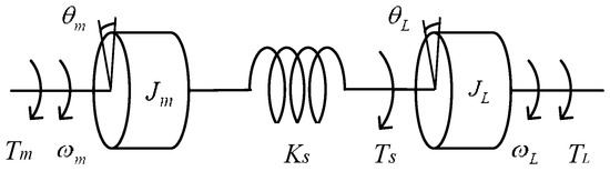
Figure 1.
Two-inertia system.
Here, and are inertial moments of motor and load (). is the torsional elastic coefficient of drive mechanism (). and are speeds of motor and load (), and and are angles of motor and load (). , , and correspond to motor torque, shaft drive torque, and disturbance ().
Dynamic equations of the two-inertia system are illustrated as follows, where the damping coefficient of the mechanical system is generally ignored due to relatively small value.
The open-loop transfer functions from motor torque to motor speed and load speed take on the following forms:
where is anti-resonant frequency, is resonant frequency, and R is the inertia ratio of load to motor.
2.2. Speed Control System
Based on the two-inertia system, IP speed control (abbreviated as IP) is depicted in Figure 2 when the switch is in the upward position. In this configuration, represents the proportional element and represents the integral element. Specifically, the proportional element acts solely on the motor speed, whereas the integral element acts on the error between the reference speed and the motor speed.
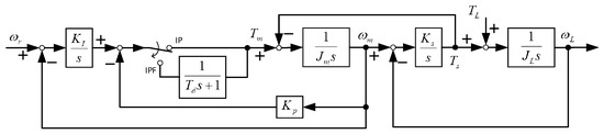
Figure 2.
Speed control systems based on IP control and IP with inertial element.
Conversely, in Figure 2, when the switch is in the downward position, IP speed control is cascaded with a first-order inertial element (abbreviated as IP with inertial element, or IPF). Meanwhile, denotes the time constant of the first-order inertial element.
3. Speed Control
3.1. IP Speed Control
The closed-loop transfer functions from reference speed to motor speed and load speed take on the following forms:
The closed-loop transfer function from the disturbance to the load speed is given by
Appling the Final Value Theorem [21], the steady state error of Formula (6) in response to a step disturbance is zero as follows:
The system is of the fourth order, while there are only two feedback parameters: and . Formula (5) can be broken down into a composition of two second-order transfer functions, as follows:
where and are angular frequencies and and are the relative damping coefficients.
By matching the coefficients of each order in Formulas (5) and (8), the following four relationships are obtained:
Here, Formulas (9) and (10) determine two control parameters and , while Formulas (11) and (12) are the constraint relations of the system parameters, so two control parameters cannot configure the four poles arbitrarily. If a meaningful constraint condition is introduced, it is possible that the pole assignment with design significance is derived by the constrained optimization.
3.2. Pole Assignment and Parameter Design
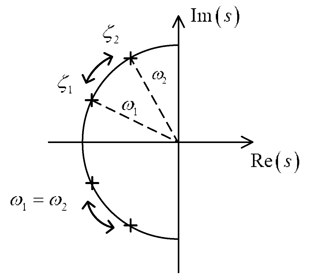
The constraint relation of the pole assignment is simplified by applying a constraint condition of identical radius. The poles are arranged along a semicircle, as shown in Figure 3; that is, .

Figure 3.
Pole placement with identical radius .
Formulas (9)–(12) are simplified as
Constraint conditions (15) and (16) are simplified significantly, and and are set as ; on the other hand, the product of and is directly constrained by the inertia ratio R. Then, one damping coefficient increases and another damping coefficient decreases, that is, the two pairs of poles move backward along the radius.
For three relatively small inertia ratios = 1, 0.75, 0.5, when or 0.5, damping coefficient is listed in Table 1, that is, is weak damping, and becomes smaller as the inertia ratio decreases.

Table 1.
for different R and
.
4. Speed Control with a First-Order Inertial Element
4.1. Speed Control with a First-Order Inertial Element
For IP with the inertial element in Figure 2, the closed-loop transfer functions from reference speed to motor and load speed take on the following forms:
The closed-loop transfer function from the disturbance to the load speed is given by
Appling the Final Value Theorem [21], the steady state error of Formula (19) in response to a step disturbance is also zero, as follows:
Formula (18) is decomposed into a combination following transfer functions:
By matching Formula (21) with (18), the following five coefficient relationships are obtained:
Formulas (22)–(24) determine the system control parameters , , and , while Formulas (25) and (26) are the constraint relations among the design parameters.
If a meaningful constraint condition is introduced, it is possible that the constrained optimization of pole assignment can be solved; furthermore, by looking for the design pointer, the effect on suppression resonance is revealed.
4.2. Pole Assignment
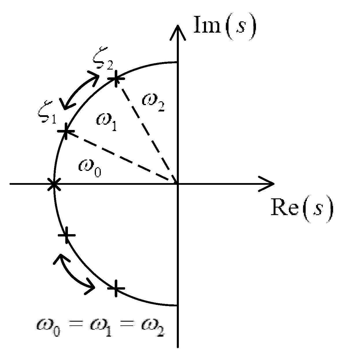
An intuitive feature with design significance is desired; learning from the design idea of the identical radius pole assignment in the previous section, the system poles are lined up along a semicircle, as shown in Figure 4. That is,

Figure 4.
Pole placement with identical radius .
Formulas (20)–(24) are simplified as
Furthermore, the explicit relationships can be derived from Formulas (31) and (32) as
The constraint relationship between and in Formula (34) indicates that will decrease as increases; that is, the two pairs of poles move in reverse along the radius.
Furthermore, is obtained, and since both and are in the range of [0, 1], then R must be within
From the discussions in Section 3, underdamping occurs at a relatively small inertia ratio, e.g., , and then the derived boundary of the inertia ratio in Formula (35) is useful enough since it completely covers the range of the relatively small inertia ratio.
Moreover, without losing of generality, assuming that , then from Formula (34), the damping coefficient must be set as
The design examples are presented while the inertia ratio R is set as 1, 0.75, and 0.5, respectively; the setting range of the in Formula (36) is given in Table 2. That is, the damping coefficient has a wide setting range, and it can be set to be within [0.707, 1].
Table 2.
Setting range of for different R.
The design process is summarized as follows.
For inertia ratio R, the damping coefficient is set via Formula (36), and the damping coefficient is obtained by Formula (34). Next, , , and are given by Formulas (27) and (33), and then , , and are obtained from Formulas (28)–(30) directly.
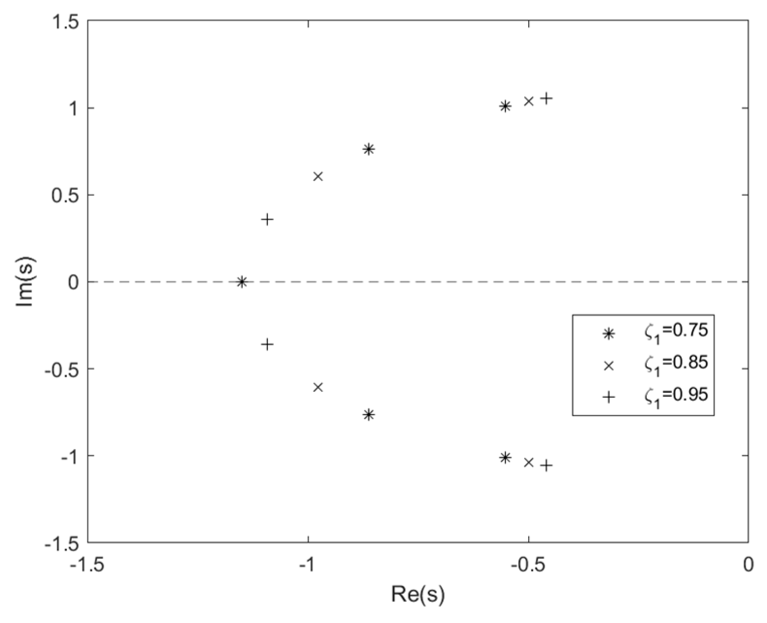
Without losing generality, the anti-resonant frequency is normalized as 1 rad/s. The design example for is analyzed, while is set as 0.75, 0.85, and 0.95, respectively, and system parameters are shown in Table 3; that is, decreases slightly as increases.
Table 3.
System design parameters ().
Furthermore, the pole distribution in Table 3 is shown in Figure 5, and the step responses of the system are given in Figure 6; as a result, the system shows a stable and smooth response.
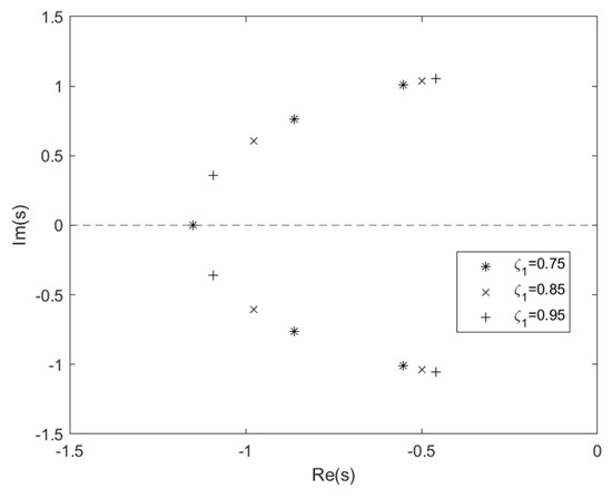
Figure 5.
Pole distribution (R = 0.75).
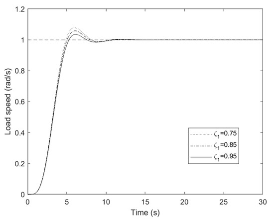
Figure 6.
Step responses (R = 0.75).
5. Mechanism for Performance Improvement
The system damping characteristic is compared; for the convenience of analyzing damping performance, the coefficient is kept at the same value for IP control and IP with inertial element, and then another damping coefficient can be used to valuate straightforwardly.
5.1. Comparison of Damping Characteristics
The damping coefficients for two controls are calculated by Formulas (16) and (34) separately, and their difference is as follows:
where represents the relative damping coefficient with IP control. The above formula is expanded:
Owing to Formula (36), the denominator term in Formula (38) is greater than 0, and the first term in numerator is also greater than 0. The second term in the numerator is also greater than 0, since both R and are positive real numbers, and then . This indicates that is inevitable, i.e, IP with an inertial element always provides a greater damping coefficient than IP control.
For three inertia ratios, R = 1, 0.75, and 0.5, damping coefficient is set as 0.75, 0.85, and 0.95, respectively. The damping coefficient is listed in Table 4, and in IP with the inertial element is nearly twice as much as the one in IP control.
Table 4.
Comparison of for IP control and IP with inertial element (IPF).
5.2. Comparison of Pole Distributions
The difference in the pole radius for two controls is obtained from Formulas (15) and (33) directly:
where
represents the pole angular frequency
with IP control. Since the inertia ratio R is a positive number, then ; that is, the pole radius in IP with the inertial element is larger than the one in IP. For R = 0.5, 0.75, and 1, the pole radii are listed in Table 5.
Table 5.
Comparison of for IP control and IP with inertial element (IPF).
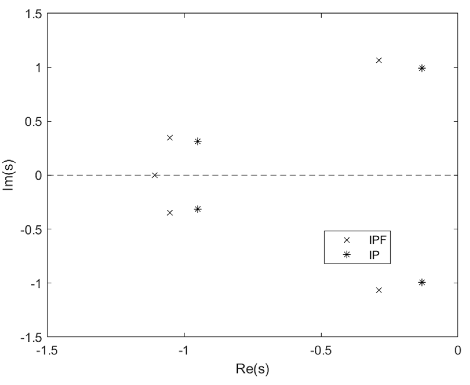
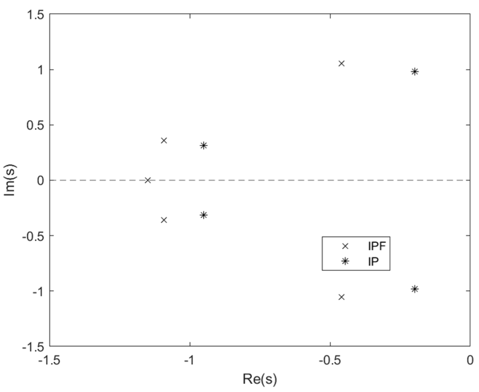
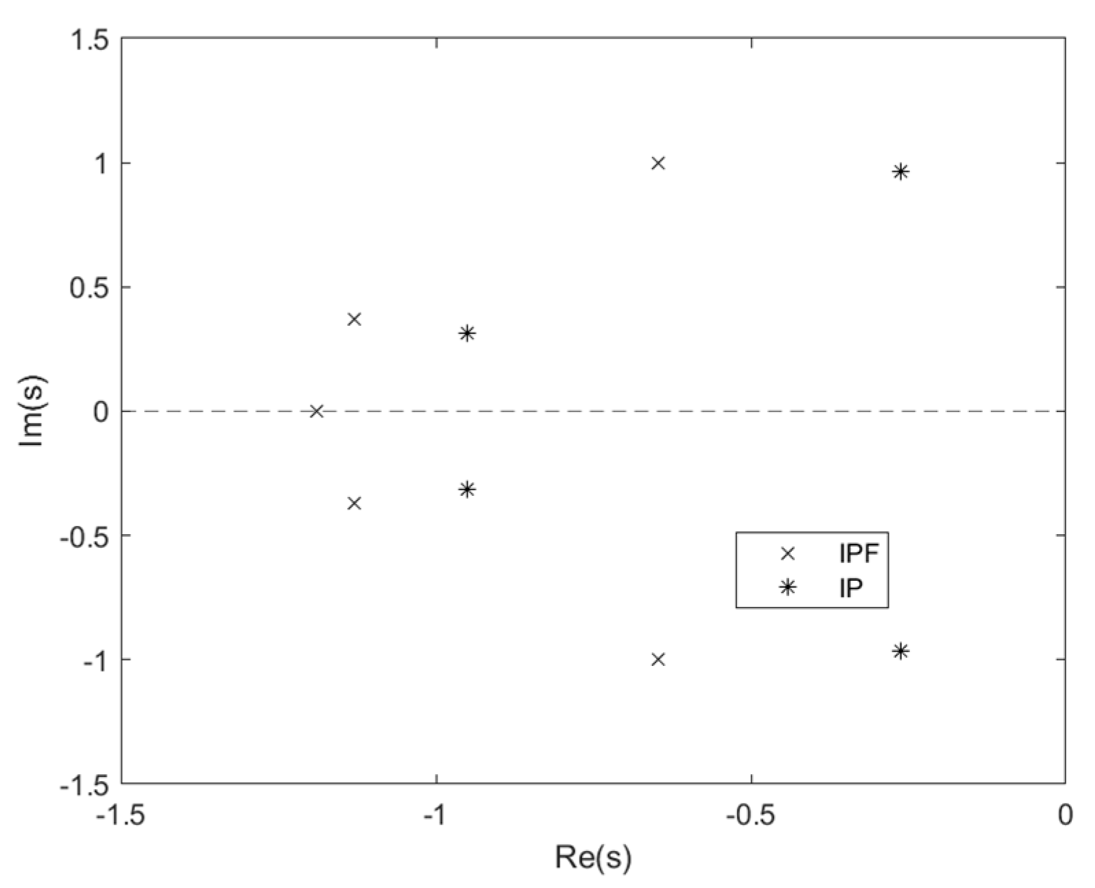
The effect of pole distributions is analyzed and compared, without losing generality, and the anti-resonant frequency is normalized as 1 rad/s. For R = 0.5, 0.75, 1, and , the pole distributions for two controls are shown in Figure 7, Figure 8 and Figure 9, that is, the poles of IP with inertial element (IPF) are farther from the imaginary axis than those of IP control, i.e, the inertial element can enhance the damping of IP control.

Figure 7.
Pole distribution (R = 0.5).
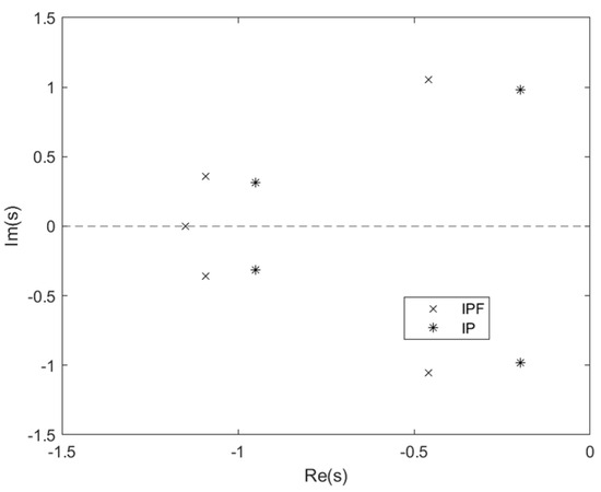
Figure 8.
Pole distribution (R = 0.75).

Figure 9.
Pole distribution (R = 1).
5.3. Simulation Comparison
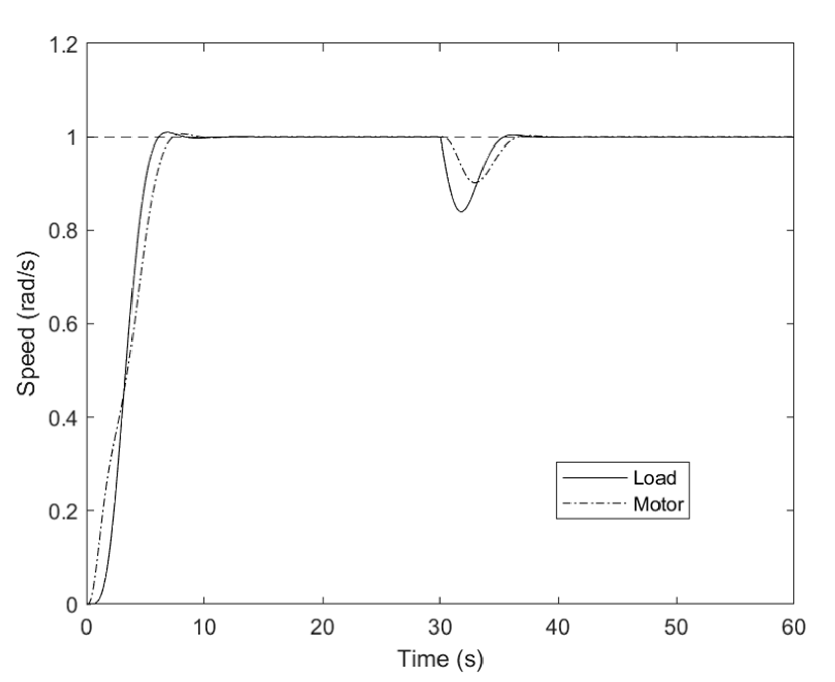
The effect of damping is compared through the step responses of both reference speed and disturbance. Based on the pole assignment in Figure 9, the step responses of motor and load speeds are obtained in Figure 10 and Figure 11, while the disturbance torque is imposed at 30 s. It is clearly shown that the dynamic change and fluctuation of both motor and load speeds by IP with inertial element are lower than those with IP control. Since the dynamic change and the fluctuation of speed reflect damping characteristics of torsional vibration, then system damping is effectively enhanced by adding the inertial element.
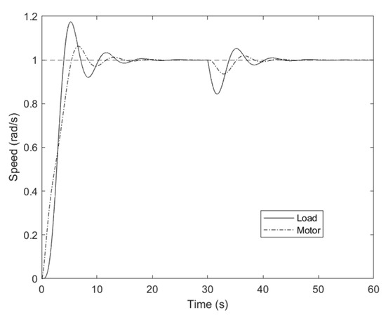
Figure 10.
Simulation of speed responses for IP control (R = 1).
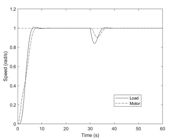
Figure 11.
Speed responses for IP with inertial element (R = 1).
6. Experimental Section
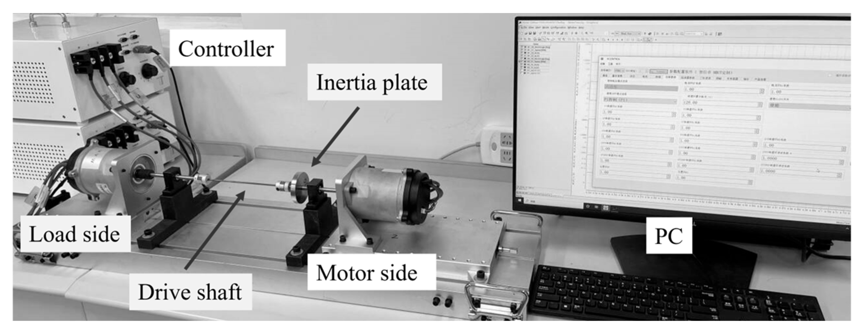
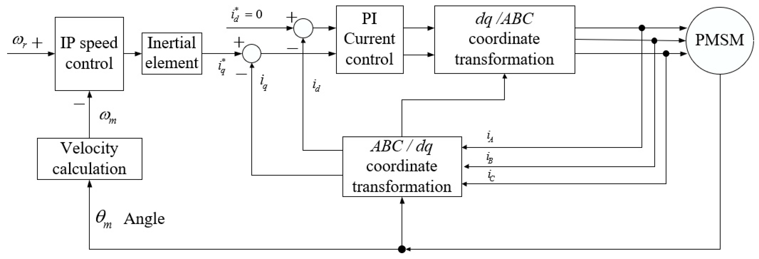
The experimental platform of the two-inertia system is shown in Figure 12, with two surface-mounted permanent-magnet synchronous motors [28]; the motor control diagram is shown in Figure 13, where the current inner-loop is the PI control of the motor d-q axis, and the outer loop is speed control.

Figure 12.
Experimental platform.
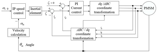
Figure 13.
Motor control diagram.
The MR sensor inside the motor is used to sense the motor angle, and motor speed is calculated by a differential calculation of the motor angle. The two motors are the same, and they are connected by a flexible drive shaft. One motor is used as the driving motor, and another motor is used as the load, which can also impose torque disturbance. The inertia plate can be installed and fixed on the shaft of the motor or load side freely, and then the inertia ratio between the load side and the motor side can be configured by changing the inertia plate.
The main parameters of the experimental system are shown in Table 6, where the torsional elastic coefficient of the shaft is about 2.33 ().
Table 6.
Experimental parameters of the two-inertia system.
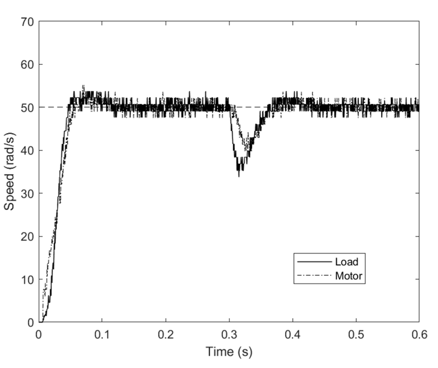
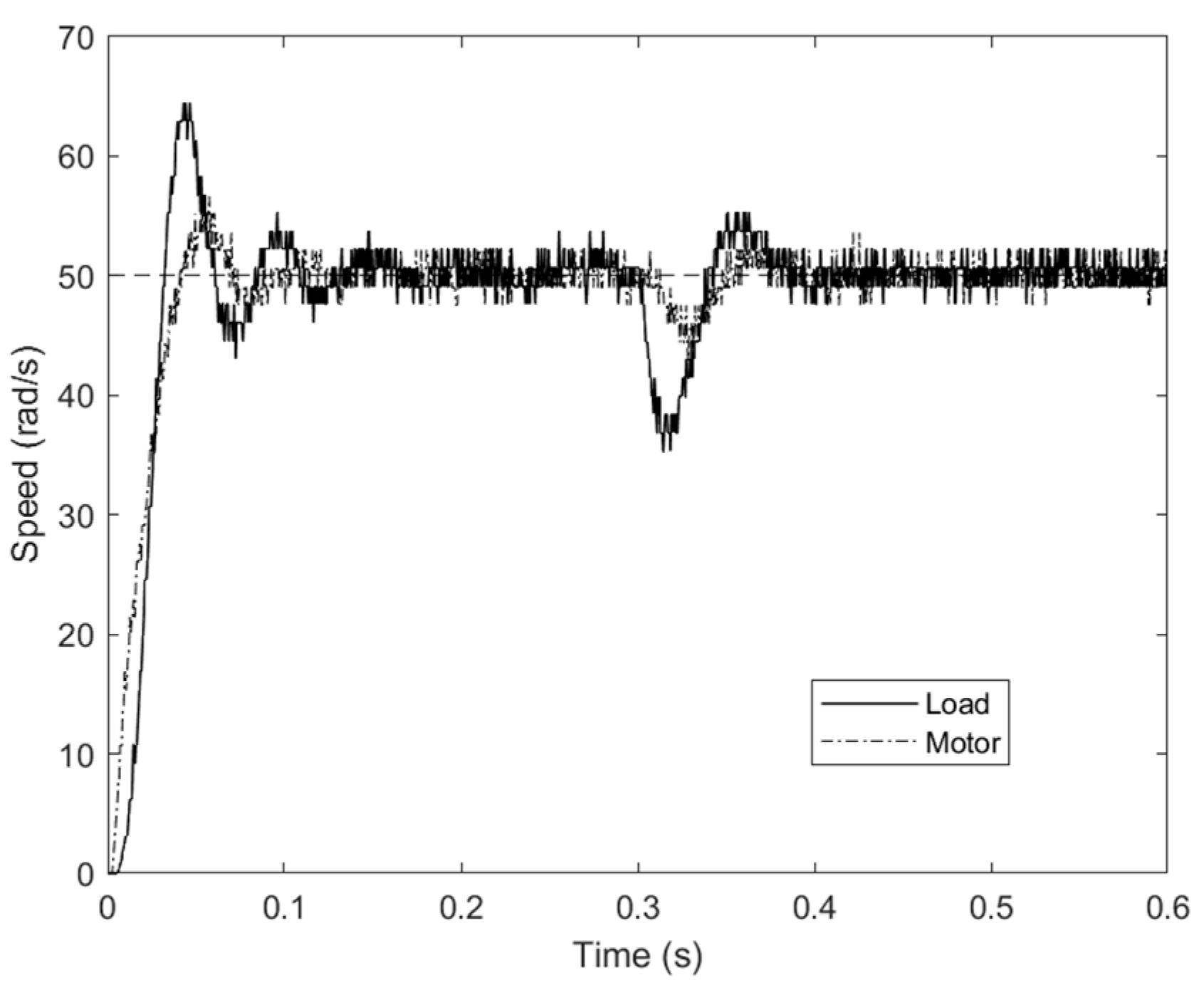
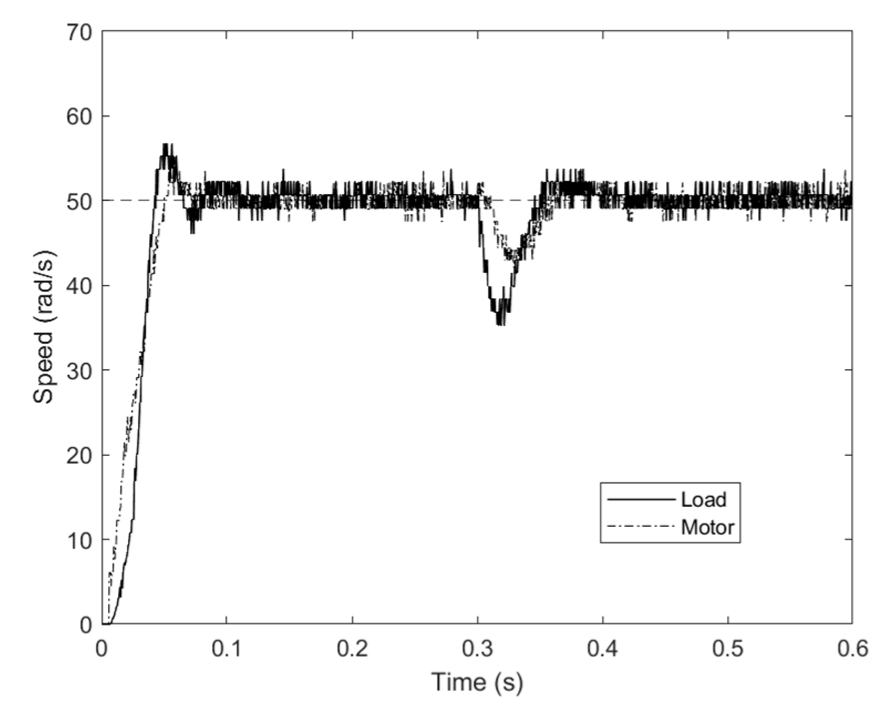
Experimental tests for IP control and IP with inertial element are carried out, while the reference speed of the drive motor is 50 rad/s, and the torque disturbance is imposed at 0.3 s. For inertia ratio R = 1, the experimental results of motor and load speeds are shown in Figure 14 and Figure 15; these results are basically consistent with the simulations.
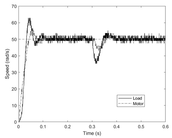
Figure 14.
Speed responses for IP control (R = 1).

Figure 15.
Speed responses for IP with inertial element (R = 1).
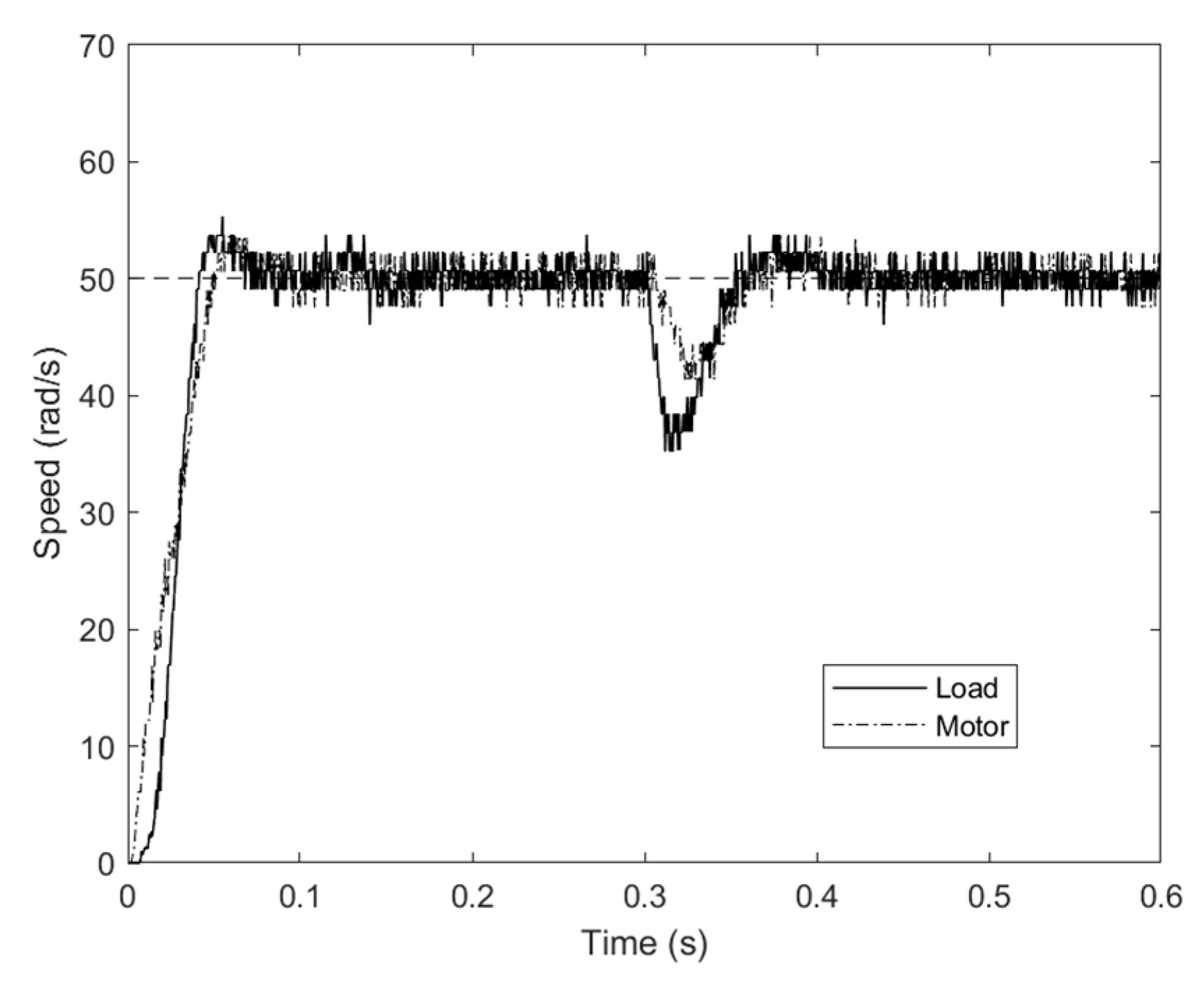
For inertia ratios R = 0.73 and 0.56, the experimental results of motor and load speeds are also given in Figure 16, Figure 17, Figure 18 and Figure 19. That is, the dynamic change and fluctuation of motor and load speeds for IP with the inertial element are significantly lower than those for IP control.
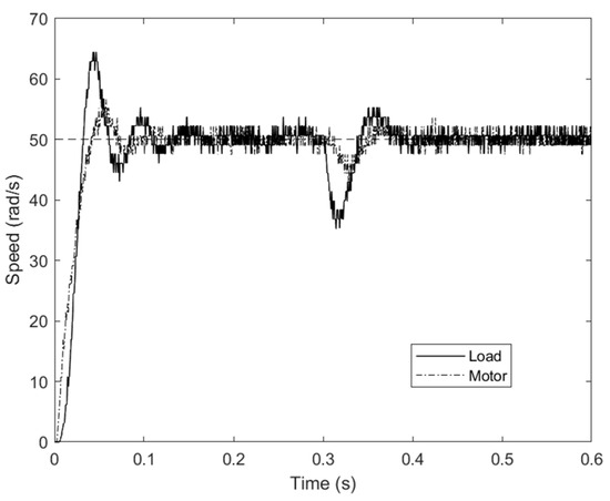
Figure 16.
Speed responses for IP control (R = 0.73).
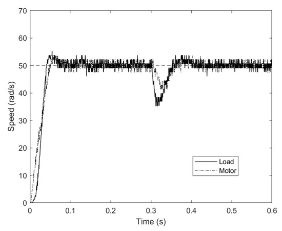
Figure 17.
Speed responses for IP with inertial element (R = 0.73).
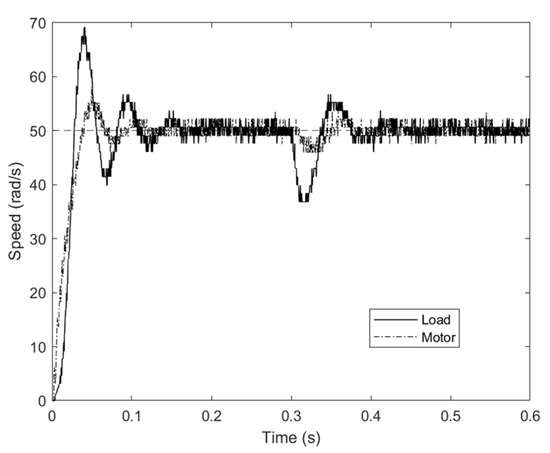
Figure 18.
Speed responses for IP control (R = 0.56).

Figure 19.
Speed responses for IP with inertial element (R = 0.56).
Settling time is used to evaluate the transient effect of damping suppression, while the settling time is defined as the time required for the response curve to reach and stay within the absolute 5% range about the final value. The settling times in Figure 14, Figure 15, Figure 16, Figure 17, Figure 18 and Figure 19 are listed in Table 7; due to the 5% range limitation and the presence of noise in the experimental data, this generally reflects the transient change. In general, the setting times for both reference speed and disturbance are significantly shortened for IP with the inertial element.
Table 7.
Setting times for IP control and IP with inertial element (IPF).
7. A Comprehensive Comparison of Control Strategy
Based on the PI/IP speed control on the two-inertia system, a comprehensive comparison table of the PI/IP “+” control strategies is included in Table 8, and the main superiorities and application boundary of this work are as follows:
- Regarding the first-order inertial element, there is no need for additional feedback as state feedback or derivative computation as PID control. Moreover, the order of the inertial element is lower than that of a notch filter.
- IP with a first-order inertial element can effectively enhance system damping for IP control. Although there is a boundary for the inertia ratio in Formula (35), the boundary is useful enough since it completely covers the range of the relatively small inertia ratio for application.
Table 8.
A comprehensive comparison table of different control strategies.
Table 8.
A comprehensive comparison table of different control strategies.
| Control Strategy | Feedback Parameters | System Order | Issues or Limitations in Application | |
|---|---|---|---|---|
| PI/IP | two | fourth order | limited performance and underdamping at relatively small ratio | |
| PI/IP “+” | State feedback | three or more | fourth order | sensor cost |
| Notch filter | three or more | fourth order | Non-additional feedback, sensitive to resonance characteristic | |
| Derivative (D) | three | fourth order | sensitive to derivative computation | |
| Inertial element | three | fifth order | Non-additional feedback, no derivative computation as PID, damping improvement but limited-scope inertial ratio in Formula (35) | |
8. Conclusions
For a two-inertia system, the IP speed control system shows an underdamping characteristic when the inertia ratio is relatively small. To improve damping, an IP speed control scheme cascaded with a first-order inertial element is introduced, and the design approach based on the constrained optimization of pole assignment is proposed. By revealing the design implication of pole assignment with an identical radius, the constraint conditions are substantially simplified, and the control parameters and damping coefficients can be directly obtained in an analytical form, so the effects of vibration suppression are quantitatively elucidated.
Theoretical analyses and design comparisons are carried out in relation to IP control and IP with a first-order inertial element, and it is shown that the inertial element can effectively enhance system damping. Design guidelines for pole assignment and its constrained optimization are proposed, and the applicable boundary for the inertial element is theoretically defined.
The derived equations and the control parameters have clear design rules; they are intuitive and highly practical. Finally, experiments are conducted to validate the effectiveness of the proposed control and design methods.
Author Contributions
Conceptualization, G.Z.; methodology, G.Z. and S.X.; software, S.X. and G.Z.; validation, G.Z. and S.X. and P.H.; formal analysis, G.Z., S.X. and P.H.; investigation, G.Z., S.X. and X.W.; resources, G.Z., P.H. and X.W.; data curation, G.Z. and S.X.; writing—original draft preparation, S.X. and G.Z.; writing—review and editing, G.Z. and S.X.; visualization, G.Z. and P.H.; supervision, G.Z.; project administration, G.Z., P.H. and X.W.; funding acquisition, G.Z. All authors have read and agreed to the published version of the manuscript.
Funding
This work was supported by the Technology Innovation Program of Hubei under Grant 2024BAB088.
Data Availability Statement
The original contributions presented in this study are included in the article. Further inquiries can be directed to the corresponding author.
Conflicts of Interest
The authors declare no conflict of interest.
References
- Zhang, G.; Furusho, J. Speed control of two-inertia system by PI/PID control. IEEE Trans. Ind. Electron. 2000, 47, 603–609. [Google Scholar] [CrossRef]
- Zhang, G.; Furusho, J. Control of robot arms using joint torque sensors. IEEE Control Syst. Mag. 1998, 18, 48–55. [Google Scholar]
- Li, X.; Shang, D.; Li, H.; Li, F. Resonant Suppression Method Based on PI control for Serial Manipulator Servo Drive System. Sci. Prog. 2020, 103, 1–29. [Google Scholar] [CrossRef]
- Moberg, S.; Öhr, J.; Gunnarsson, S. A Benchmark Problem for Robust Feedback Control of a Flexible Manipulator. IEEE Trans. Control Syst. Technol. 2009, 17, 1398–1405. [Google Scholar] [CrossRef]
- Franklin, G.F.; Powell, J.D.; Emami-Naeini, A. Feedback Control of Dynamic Systems, 7th ed.; Pearson Higher Education, Inc.: New York, NY, USA, 2015; Chapter 10. [Google Scholar]
- Wang, D.; Zhang, S.; Wang, L.; Liu, Y. Developing A Ball Screw Drive System of High-Speed Machine Tool Considering Dynamics. IEEE Trans. Ind. Electron. 2022, 69, 2966–2976. [Google Scholar] [CrossRef]
- Kambrath, J.K.; Wang, Y.; Yoon, Y.J.; Alexander, A.A.; Liu, X.; Wilson, G.; Gajanayake, C.J.; Gupta, A.K. Modeling and Control of Marine Diesel Generator System with Active Protection. IEEE Trans. Transp. Electrif. 2018, 4, 249–271. [Google Scholar] [CrossRef]
- Kambrath, J.K.; Khan, M.S.U.; Wang, Y.; Maswood, A.I.; Yoon, Y.J. A Novel Control Technique to Reduce the Effects of Torsional Interaction in Wind Turbine System. IEEE J. Emerg. Sel. Top. Power Electron. 2019, 7, 2090–2105. [Google Scholar] [CrossRef]
- O’Sullivan, M.; Bingham, C.M.; Schofield, N. High-Performance Control of Dual-Inertia Servo-Drive Systems Using Low-Cost Integrated SAW Torque Transducers. IEEE Trans. Ind. Electron. 2006, 53, 1226–1237. [Google Scholar] [CrossRef]
- Kai, T.; Sekiguchi, H.; Ikeda, H. Relative Vibration Suppression in a Position Machines with Acceleration Feedback control. IEEJ J. Ind. Appl. 2018, 7, 15–21. [Google Scholar]
- Thomsen, S.; Hoffmann, N.; Fuchs, F.W. PI Control, PI-Based State Space Control, and Model-Based Predictive Control for Drive Systems With Elastically Coupled Loads—A Comparative Study. IEEE Trans. Ind. Electron. 2011, 58, 3647–3657. [Google Scholar] [CrossRef]
- Szabat, K.; Orlowska-Kowalska, T. Vibration suppression in a two-mass drive system using PI speed controller and additional feedbacks—Comparative study. IEEE Trans. Ind. Electron. 2007, 54, 1193–1206. [Google Scholar] [CrossRef]
- Saarakkala, S.E.; Hinkkanen, M. State-Space Speed Control of Two-Mass Mechanical Systems: Analytical Tuning and Experimental Evaluation. IEEE Trans. Ind. Appl. 2014, 50, 3428–3437. [Google Scholar] [CrossRef]
- Szabat, K.; Orlowska-Kowalska, T.; Dybkowski, M. Indirect adaptive control of induction motor drive system with an elastic coupling. IEEE Trans. Ind. Electron. 2009, 56, 4038–4042. [Google Scholar] [CrossRef]
- Szabat, K.; Than-Van, T.; Kaminski, M. A modified fuzzy luenberger observer for a two-mass drive system. IEEE Trans. Ind. Inform. 2015, 11, 531–539. [Google Scholar] [CrossRef]
- Li, P.; Duan, G.R. High-Order Fully Actuated Control Approaches of Flexible Servo Systems Based on Singular Perturbation Theory. IEEE/ASME Trans. Mechatron. 2023, 28, 3386–3399. [Google Scholar] [CrossRef]
- Wang, S.; Na, J.; Chen, Q. Adaptive Predefined Performance Sliding Mode Control of Motor Driving Systems with Disturbances. IEEE Trans. Energy Convers. 2021, 31, 1931–1939. [Google Scholar] [CrossRef]
- Jung, H.; Jeon, K.; Kang, J.; Oh, S. Iterative Feedback Tuning of Cascade Control of Two-Inertia System. IEEE Control Syst. Lett. 2021, 5, 785–790. [Google Scholar] [CrossRef]
- Szabat, K.; Wróbel, K.; Dróżdż, K.; Janiszewski, D.; Pajchrowski, T.; Wójcik, A. A Fuzzy Unscented Kalman Filter in the Adaptive Control System of a Drive System with a Flexible Joint. Energies 2020, 13, 2056. [Google Scholar] [CrossRef]
- Szczepanski, R.; Kaminski, M.; Tarczewski, T. Auto-Tuning Process of State Feedback Speed Controller Applied for Two-Mass System. Energies 2020, 13, 3067. [Google Scholar] [CrossRef]
- Ogata, K. Modern Control Engineering, 5th ed.; Pearson Hall Inc.: New York, NY, USA, 2010; Chapter 8. [Google Scholar]
- Chen, Y.; Yang, M.; Long, J.; Hu, K.; Xu, D.; Blaabjerg, F. Analysis of Oscillation Frequency Deviation in Elastic Coupling Digital Drive System and Robust Notch Filter Strategy. IEEE Trans. Ind. Electron. 2019, 66, 90–101. [Google Scholar] [CrossRef]
- Chen, Y.; Yang, M.; Sun, Y.; Long, J.; Xu, D.; Blaabjerg, F. A Modified Bi-Quad Filter Tuning Strategy for Mechanical Resonance Suppression in Industrial Servo Drive Systems. IEEE Trans. Power Electron. 2021, 36, 10395–10408. [Google Scholar] [CrossRef]
- Sonzogni, G.; Mazzoleni, M.; Polver, M.; Ferramosca, A.; Previdi, F. Notch filter design with stability guarantees for mechanical resonance suppression in SISO LTI two-mass drive systems. In Proceedings of the 2023 62nd IEEE Conference on Decision and Control (CDC), Singapore, 13–15 December 2023; pp. 7745–7750. [Google Scholar]
- Ma, C.; Cao, J.; Qiao, Y. Polynomial-method-based design of low-order controllers for two-mass systems. IEEE Trans. Ind. Electron. 2013, 60, 969–978. [Google Scholar] [CrossRef]
- Yang, Y.; Liu, C.; Lai, S.; Chen, Z.; Chen, L. Frequency-dependent equivalent impedance analysis for optimizing vehicle inertial suspensions. Nonlinear Dyn. 2024, 113, 9373–9398. [Google Scholar] [CrossRef]
- Graham, D.; Lathrop, R.C. The Synthesis of “Optimum” Transient Response: Criteria and Standard Forms. Trans. Am. Inst. Electr. Eng. Part II Appl. Ind. 1953, 72, 273–288. [Google Scholar] [CrossRef]
- Zhang, G.; Hou, P. Optimization Design of Cogging Torque for Electric Power Steering Motors. Machines 2024, 12, 517. [Google Scholar] [CrossRef]


Disclaimer/Publisher’s Note: The statements, opinions and data contained in all publications are solely those of the individual author(s) and contributor(s) and not of MDPI and/or the editor(s). MDPI and/or the editor(s) disclaim responsibility for any injury to people or property resulting from any ideas, methods, instructions or products referred to in the content. |
© 2025 by the authors. Licensee MDPI, Basel, Switzerland. This article is an open access article distributed under the terms and conditions of the Creative Commons Attribution (CC BY) license (https://creativecommons.org/licenses/by/4.0/).