Uniform Coverage Trajectory Planning for Polishing of Equation-Free Surfaces

Abstract

Conventional surface polishing trajectory generation relies on solving the plane trajectory equation in conjunction with the surface equation to obtain a surface polishing trajectory when the surface equation is known. However, in practical polishing processes, there exist equation-free surfaces which cannot be described by equations and the generation of polishing trajectories on equation-free surfaces cannot be realized by an equation-solving strategy. In this paper, a polishing trajectory generation method for equation-free surfaces modeled by meshes based on the trajectory mapping strategy is proposed. As the calculation process for the coverage area of polishing trajectories requires invoking surface curvature information, this paper proposes a mesh surface curvature fitting algorithm. Regarding the problem of non-uniformity in the coverage area of polishing trajectories caused by surface curvature fluctuations, an algorithm for adjusting the position of polishing trajectory points on mesh surfaces is proposed, which enables the mapped trajectory points to be adjusted according to the required overlapping coverage area of the adjacent polishing trajectories. The uniform coverage of multiple polishing trajectories for rotationally symmetric workpieces is achieved by the proposed trajectory point position adjustment algorithm. Through experiment and analysis, it is verified that the proposed algorithm for uniform coverage of polishing trajectories can obtain better polishing results with the same polishing time.

1. Introduction

Trajectory planning is the prerequisite for achieving deterministic polishing [1]. Traditional trajectory planning for surface machining mostly uses the iso-parametric method [2], iso-planar method [3], and iso-scallop method [4]. The iso-parametric method generates a machining path along one parameter of the surface S(u,v) by keeping another parameter of the surface unchanged (i.e., one of the parameters u or v remains unchanged). This low-computation method is usually used for trajectory planning of simple surfaces, but it can only obtain simple machining trajectories. The iso-planar method uses several equally spaced parallel planes to intersect the surface being machined, and the intersection line of each plane with the surface being machined is used as the machining trajectory. This method can be used to generate the machining trajectory for more complex surfaces, but the disadvantage lies in the excessive computation when the surface model is large. The iso-scallop method takes any surface boundary as the initial machining path, and the next trajectory is calculated based on the tool contact on the current trajectory. The iso-scallop method is a dynamic trajectory planning method, but the calculation process is more complicated and time-consuming.

Although the above trajectory planning methods can realize the generation of polishing trajectories for simple curved surfaces, they are unable to consider the influence of surface curvature on the trajectory spacing, which leads to inconsistency in material removal and fails to obtain excellent machining quality.

The conventional research on polishing trajectories of complex surfaces can be divided into two principal categories. The first category concerns the use of interpolation and other methods to achieve the acquisition of polishing trajectories [5]. The second category is concerned with optimizing the processing parameters of simple polishing trajectories with a view to improving polishing quality [6]. Zhao et al. [7] implemented a systematic NURBS (Non uniform rational B-spline) interpolation method for polishing trajectory planning, leveraging Successive Over-Relaxation (SOR) iteration theory to reduce the computational difficulty of control point solving. Han et al. [8] achieved parametric trajectory interpolation by integrating NURBS curves with the Milne–Hamming predictor-corrector algorithm. Zhang et al. [9] proposed an adaptive trajectory planning method based on NURBS interpolation principles and incorporating a finite element model of the tool-blade contact as a constraint, enabling uniform blade polishing. Chen et al. [10] developed a high-precision motion interpolation method combining a fourth-order Runge–Kutta adaptive algorithm (RK4) with variable-feed velocity planning (VF), addressing the accuracy limitations of traditional interpolation methods on open small multi-axis polishing machines. Xu et al. [11] achieved smooth machining trajectories on bi-NURBS regular surfaces by incorporating geodesic curvature and surface convexity/concavity, generating non-redundant and interference-free paths. Ren et al. [12] employed NURBS interpolation to resolve trajectory discontinuity issues encountered when machining sharp edges with parametric segmented paths. Cui et al. [13] introduced a zoned polishing trajectory generation method for complex optical surfaces based on curvature characteristics and Freeman coding. To enhance material removal uniformity and suppress edge effects during NURBS surface polishing, Han et al. [14] proposed a spiral trajectory planning method utilizing an iterative approximation algorithm. Cao et al. [15] analyzed the impact of polishing contact area, curvature, and tool attitude angle on material removal. By introducing curvature fluctuation constraints into NURBS interpolation, they improved the material removal precision of spiral polishing paths. Xiao et al. [16] addressed trajectory planning for complex workpieces by proposing a path co-optimization method. Finally, Zheng et al. [17] experimentally quantified the influence of scanning pitch and polishing mode (e.g., transverse vs. cross-scanning) on polishing quality and efficiency. Their results confirmed that the cross-scanning mode optimizes surface integrity and identified the optimal parameter combination for achieving ultra-smooth surfaces. Wahballa et al. [18] developed a robotic polishing trajectory planning strategy integrating NURBS-S curve smoothing, gravity compensation control, and material removal depth modeling. This approach enables uniform material removal under precisely controlled constant force conditions. Huang et al. [19] constructed parametric polishing paths using cubic B-splines, establishing a one-to-one correspondence between path segments and dwell points, and further optimized trajectory interpolation via an equal-proportion feed strategy to enhance the stability of material removal. Kakinuma et al. [20] proposed a real-time polishing trajectory optimization method utilizing sensor-less force control technology and a decoupling-capable quarry matrix. This technique facilitates collaborative control of trajectory spacing, tool posture, and polishing force. Wang et al. [21] generated polishing trajectories by projecting conventional machining paths onto 3D vibration trajectories, achieving effective trajectory planning specifically for harmonic mesh surfaces. Li et al. [22] obtained random-like Lissajous polishing trajectories through controlled vibration parameter modulation, effectively addressing the issue of periodic polishing marks on workpiece surfaces caused by traditional circular/elliptical trajectories in small-tool polishing.

The above studies have focused on the generation of complex surface machining trajectories for which the surface equations are known or the optimization of existing polishing trajectories to meet specific polishing requirements in certain cases. Therefore, there are evident limitations in terms of general applicability. Benefiting from the development of computer graphics, the mathematical properties of equation-free surfaces can be discretely represented by the mesh model that corresponds to the surface model. This method can solve the problem of obtaining mathematical relations of the equation-free surfaces in the machining trajectory planning process.

Although equation-free surfaces are complex surfaces that are difficult to describe with mathematical equations, the surface information can be discretely represented by triangular mesh surfaces. Triangular mesh surfaces have the following advantages in the field of trajectory planning: Triangular meshes can accurately approximate complex geometries, even on surfaces with curvature mutations. Compared to rectangular or other types of meshes, triangular meshes are able to adapt more flexibly to irregular shapes, which is especially important for trajectory planning on complex surfaces. Triangles are the simplest polygons in geometry; using triangular meshes for trajectory generation will not only simplify the computation, but also increase the computational efficiency. Since triangles consist of only three vertices and three edges, they can generate smooth surface approximations on complex surfaces, which makes it possible to generate trajectories with better continuity and smoothness on complex surfaces. Triangular meshes are widely used in 3D modeling, computer graphics, and numerical analysis, and it is easier to migrate data between different software using triangular meshes. Triangular meshes are more stable when dealing with topological changes such as mesh refinement. Through mesh subdivision and optimization, the accuracy of trajectory planning can be improved while maintaining the original geometric features. Kim et al. [23] verified the feasibility of using mesh surfaces for machining trajectory planning. Wang et al. [24] proposed a machining trajectory spacing optimization algorithm applicable to mesh surfaces. Zhang et al. [25] proposed a helical cutting path generation algorithm based on a mesh surface model, which effectively improves the cutting and machining accuracy. Li et al. [26] combined mesh surface parameterization methods with component analysis to obtain iso-parametric trajectories on mesh surfaces. Zhao et al. [27] introduced geodesic curves on triangular mesh trajectory planning, and this work effectively reduced the difficulty of trajectory planning for equation-free surfaces. Xu et al. [28] proposed a trochoidal polishing trajectory generation method for equation-free surfaces based on surface parameterization principles to improve the polishing accuracy of equation-free surfaces. Liao et al. [29] proposed a tool path planning method under constant cutting load by combining a conformal mapping parametric algorithm and a variable radius hoof trajectory.

However, a critical research gap persists. Traditional methods, reliant on NURBS solutions or interpolation, cannot guarantee that the generated trajectory’s accuracy fully adapts to the polished surface—a significant drawback for precision polishing. Surface parameterization methods applied to mesh models reduce dimensionality and complexity for trajectory generation on intricate, equation-free surfaces. Nevertheless, this approach introduces two inherent challenges: (1) inevitable distortion during the mesh parameterization process, and (2) the computational burden and potential inaccuracies associated with solving the resulting nonlinear equations. Both factors compromise the final polishing trajectory precision. More importantly, and constituting a major oversight in the existing literature, achieving uniform coverage of the polishing trajectory—essential for polishing to prevent over-polishing/under-polishing, effectively suppress high-spatial frequency errors, and achieve more consistent surface outcomes within the same processing cycle–has received insufficient attention. Current research, even mesh-based, largely neglects this crucial capability.

Therefore, this paper aims to address these limitations by pursuing the following specific research objectives for trajectory generation and optimization in sub-aperture polishing (especially when employing compliant spherical tools) of equation-free optical surfaces:

• To develop a method for generating high-precision polishing trajectories on equation-free surfaces that operates directly on the mesh representation, eliminating the need for surface equation solving and the associated distortion and computational issues of parameterization;
• To design and implement an algorithm capable of optimizing polishing trajectories to achieve uniform coverage, thereby mitigating the risks of over-polishing and under-polishing and facilitating faster attainment of the desired polishing effect.

The various sections of this paper are organized as follows: In Section 2, an algorithm for generating a polishing trajectory on equation-free surfaces is proposed, and the mathematical principles of the corresponding algorithm are elucidated. In Section 3, a curvature-solving algorithm applicable to mesh surfaces is proposed for obtaining surface curvature in the calculation of the polishing contact area. The mathematical principles of the corresponding algorithm are elaborated, and the computational accuracy of the algorithm is verified. In Section 4, a polishing trajectory point adjustment algorithm on mesh surfaces is proposed and a method for achieving uniform coverage of both symmetrical and asymmetrical polishing trajectories is further proposed. The relevant mathematical principles are explained, and the feasibility of the algorithms is ultimately validated through simulations. In Section 5, experimental tests are conducted to reveal the impact of uniform coverage and non-uniform coverage polishing trajectories on the quality of polishing equation-free surfaces. The conclusions are given in Section 6.

2. Mathematical Implementation of Mapping Planar Trajectories to Mesh Surfaces

Assuming that the coordinates of three vertices in 3D space for any triangle mesh in an equation-free mesh surface are P₁(x₁,y₁,z₁), P₂(x₂,y₂,z₂) and P₃(x₃,y₃,z₃), respectively, the unit normal vector n for the triangular mesh can be calculated as Equation (1).

$$n={\displaystyle \frac{\overrightarrow{P_2-P_1}\times \overrightarrow{P_3-P_1}}{{‖\overrightarrow{P_2-P_1}\times \overrightarrow{P_3-P_1}‖}^2}}={\displaystyle \frac{V_1\times V_2}{{\Vert V_1\times V_2\Vert }^2}}$$

(1)

The vector n is decomposed along the x-axis, y-axis, and z-axis to obtain the vectors n_x, n_y, n_z. Then, the mathematical properties of the equation-free grid surface can be expressed as a discrete combination of multiple triangular grids, as shown in Equation (2).

$$S={\displaystyle \sum _{i=1}^{Num}{n}_{xi}x+n_{yi}y+n_{zi}z+d_i=0}$$

(2)

In Equation (1), the parameter ‘Num’ denotes the total number of triangular meshes within the mesh surface.

After obtaining the plane equation for any triangular mesh within the mesh surface, it is possible to further solve for the trajectory coordinates of the planar trajectory points mapped onto the mesh surface. The validity of the triangular mesh in the mapping direction should be determined firstly. (When the triangle mesh is parallel to the mapping direction, the planar trajectory points cannot intersect with the triangle mesh along the mapping direction.)

Assuming that the mapping direction is determined by the unit vector m, the coordinate components of m in the X, Y, and Z directions are m_x, m_y, and m_z, respectively. The equation of the plane F_i with vector m as the normal vector and containing the mapped point P(x₀, y₀, z₀) is m_x(x − x₀) + m_y(y − y₀) + m_z(z − z₀) = 0.

Assuming that the three vertices of any triangular mesh T_i are V₁ = (x₁,y₁,z₁), V₂ = (x₂,y₂,z₂), V₃ = (x₃,y₃,z₃), the vertices of the triangular mesh T_i after projection to the plane F_i along the opposite direction of the mapping direction are v₁, v₂, and v₃. The computation of the coordinates of the corresponding vertices can be achieved by Equation (3).

$$\left\{\begin{array}{c}{v}_1=V_1-{\displaystyle \frac{m{(V_1-P)}^T}{{‖m‖}^2}}m\\ v_2=V_2-{\displaystyle \frac{m{(V_2-P)}^T}{{‖m‖}^2}}m\\ v_3=V_3-{\displaystyle \frac{m{(V_3-P)}^T}{{‖m‖}^2}}m\end{array}\right.$$

(3)

Define the auxiliary vectors U and V, where U = v₁ − v₂ and V = v₁ − v₃. If U × V ≠ 0, the triangle mesh T_i is a valid triangle in the mapping direction.

Three results can be obtained by mapping a planar trajectory point P to a triangular mesh:

Case 1: point P can be mapped to the interior of the triangle mesh (corresponding to Figure 1a);

Case 2: point P can be mapped to an edge of the triangle mesh (corresponding to Figure 1b);

Case 3: point P cannot be mapped to the interior of the triangle mesh (corresponding to Figure 1c).

It can be intuitively seen that only in the two cases of Figure 1a,b, the point P can be mapped to the corresponding triangular mesh. In this case, the vectors $\overrightarrow{v_{1}P}$, $\overrightarrow{v_1{v}_2}$, $\overrightarrow{v_1{v}_3}$ formed by the point P and the three vertices of the triangular mesh T_i satisfy the mathematical relationship described in Equation (4).

$$\overrightarrow{v_{1}P}=r\overrightarrow{v_1{v}_2}+s\overrightarrow{v_1{v}_3}(0\le r\le 1,0\le s\le 1)$$

(4)

If the triangular mesh T_i is a valid triangle in the mapping direction, the plane equation of T_i is obtained by Equation (1), and the coordinates of the spatial point P_M obtained by mapping point P(x₀, y₀, z₀) along the direction of vector m onto triangular mesh T_i can be solved using Equation (5).

$$P_M=P-{\displaystyle \frac{[n_x(x_0-x_1)+n_y(y_0-y_1)+n_z(z_0-z_1)]}{n_x{m}_x+n_y{m}_y+n_z{m}_z}}n$$

(5)

In Equation (5), (x₁,y₁,z₁) are the coordinate values of the vertex V₁ of the triangle mesh T_i.

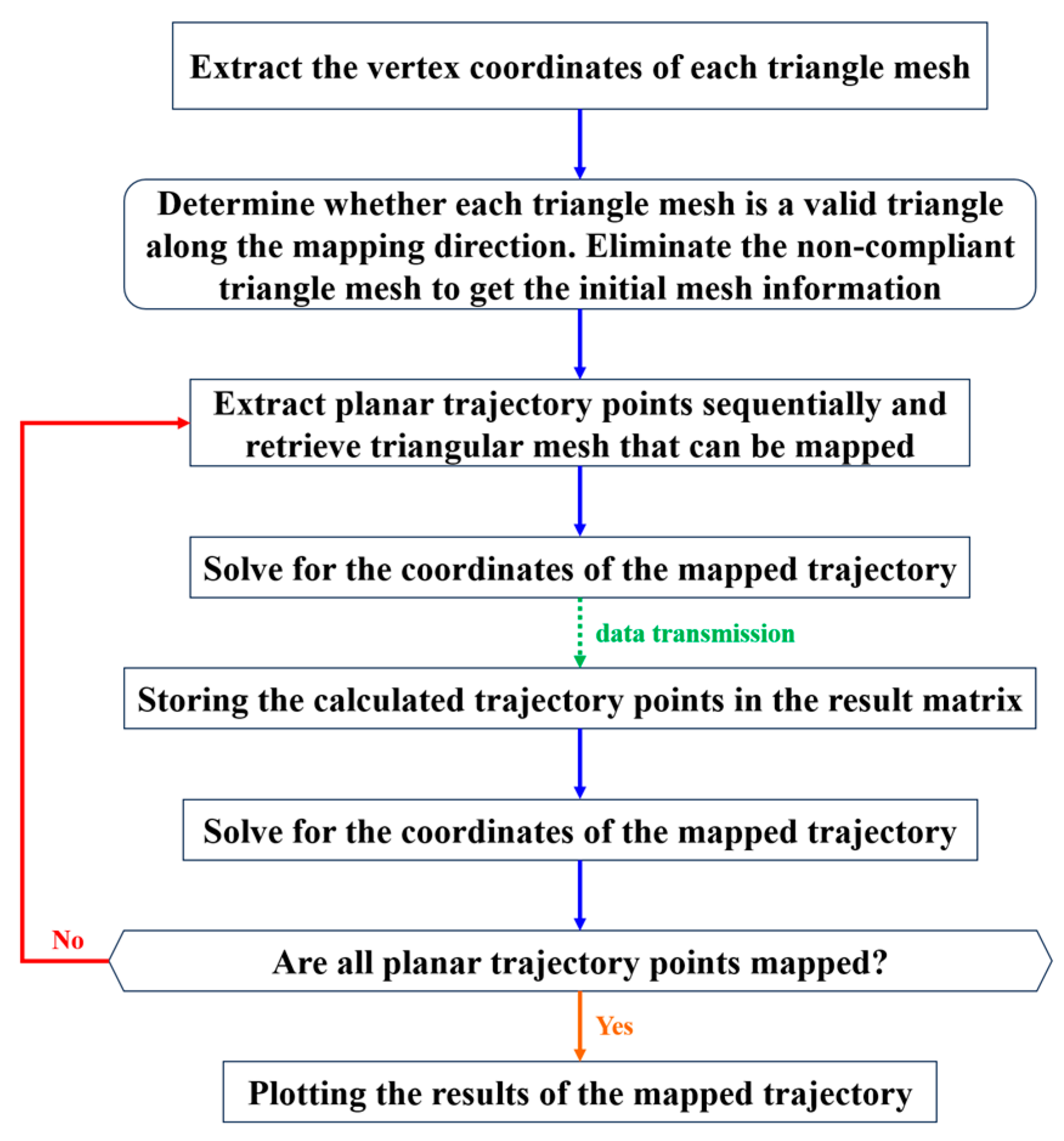
The flowchart of the mapping algorithm for planar trajectories to a mesh surface is shown in Figure 2.

According to the proposed trajectory mapping strategy, an equidistant helical trajectory on the plane is mapped onto an equation-free mesh surface with a size of 20 cm × 20 cm. The final simulation visualization result is shown in Figure 3.

3. Calculation of Curvature of Triangular Mesh Vertices Within the Mesh Surface and Curvature Fitting of Trajectory Points

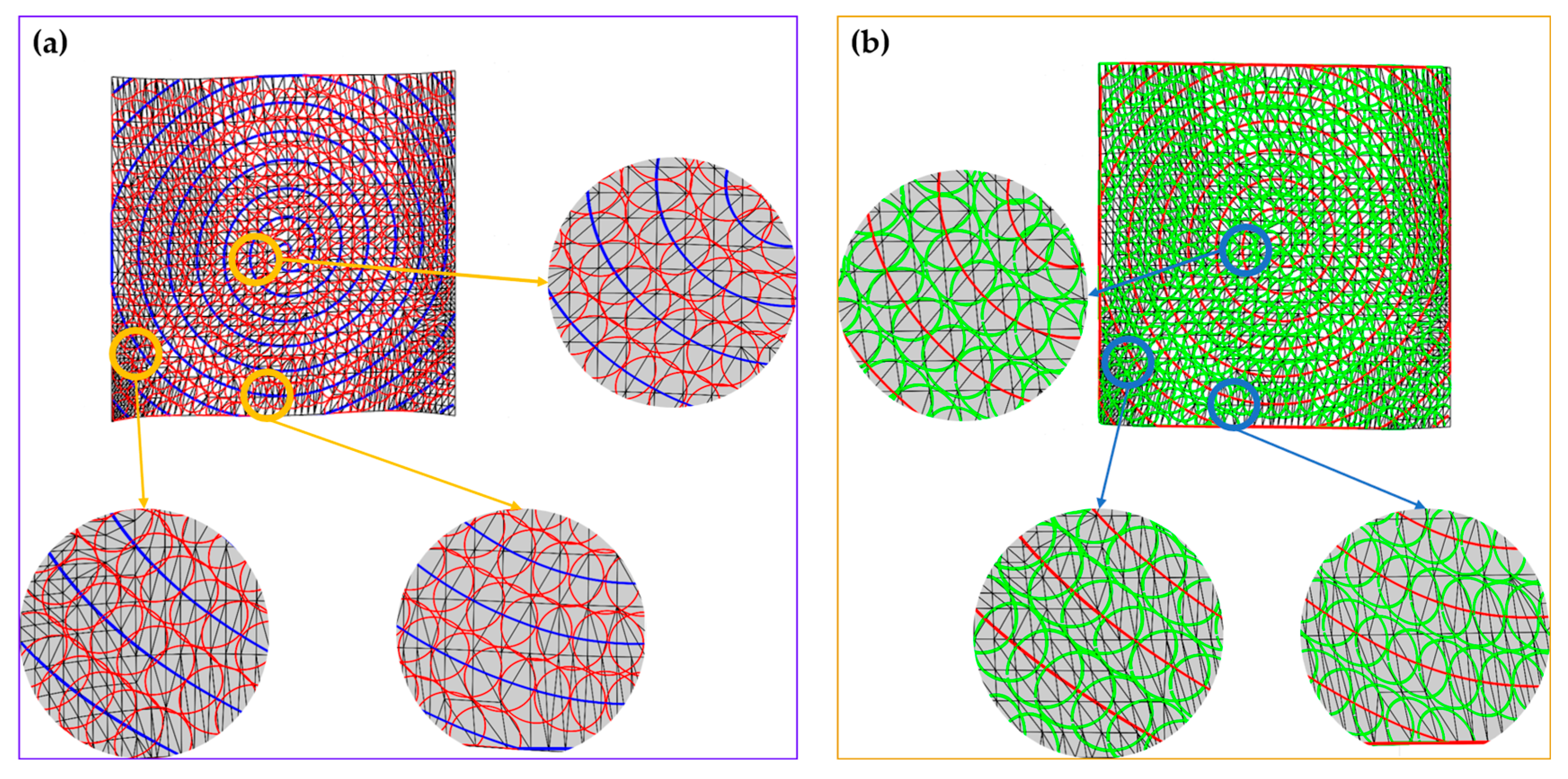
After mapping an equidistant polishing trajectory from the plane to an equation-free surface, the fluctuation in surface curvature leads to changes in the spacing of adjacent polishing trajectories, as shown in Figure 3. As shown in Figure 4a,b, the red and green circles are used to represent the contact circles of some trajectory points belonging to the successive polishing trajectory of the surface, respectively. Each contact circle reflects the size of the polished contact area at the corresponding trajectory point. According to the partially enlarged detail of Figure 4a,b, it can be seen that if the positional relationship of the polishing circles between any two adjacent polishing trajectory points is not consistent, excessive overlap area between polishing circles can lead to over-polishing, while no overlap area between polishing circles can lead to under-polishing; this ultimately affects the quality of surface polishing. Therefore, it is necessary to adjust the position of the mapped polishing trajectory points. However, adjusting the positions of polishing trajectory points requires determining the size of the polishing contact area at each trajectory point to obtain the adjustment magnitude for each trajectory point.

Under static contact conditions, the polishing contact area between the polishing tool and the surface is elliptical, and the major axis ‘a’ and minor axis ‘b’ of the corresponding elliptical region can be obtained by Equation (6) [30].

$$\left\{\begin{array}{c}a={\left({\displaystyle \frac{3k^2\epsilon QR}{\pi \tilde{E}}}\right)}^{{\displaystyle \frac{1}{3}}}\\ b={\left({\displaystyle \frac{3\epsilon QR}{\pi k\tilde{E}}}\right)}^{{\displaystyle \frac{1}{3}}}\end{array}\right.$$

(6)

In Equation (6), Q is the total contact force, $\tilde{E}$ is the equivalent modulus of elasticity, R represents the equivalent radius of the polishing tool and the polished surface, and parameters k and ε are empirical coefficients, as shown in Equations (7)–(10).

$${\displaystyle \frac{1}{\tilde{E}}}={\displaystyle \frac{1-{\mu }_1^2}{E_1}}+{\displaystyle \frac{1-{\mu }_2^2}{E_2}}$$

(7)

$$R={\displaystyle \raisebox{1ex}{$1$}\!\left/ \!\raisebox{-1ex}{${\rho }_{I1}+{\rho }_{I2}+{\rho }_{II1}+{\rho }_{II2}$}\right.}$$

(8)

$$k=1.0339{\left({\displaystyle \frac{{\rho }_{\mathrm{I}1}+{\rho }_{\mathrm{I}2}}{{\rho }_{\mathrm{II}1}+{\rho }_{\mathrm{II}2}}}\right)}^{0.636}$$

(9)

$$\epsilon =1.0003+0.5968\left({\displaystyle \frac{{\rho }_{\mathrm{II}1}+{\rho }_{\mathrm{II}2}}{{\rho }_{\mathrm{I}1}+{\rho }_{\mathrm{I}2}}}\right)$$

(10)

In Equation (7), E₁ and E₂ are the modulus of elasticity of the polishing tool and the polished surface, respectively, and μ₁ and μ₂ are the Poisson’s ratios of the polishing tool and the polished surface, respectively. In Equations (7)–(10), ρ_I1 and ρ_I2 represent the principal and subsidiary curvatures of the polishing tool, and ρ_II1 and ρ_II2 represent the principal and subsidiary curvatures of the polished surface.

Adjustment of the position of the mapped trajectory points requires a specific amount of adjustment depending on the size of the polished contact area. During the polishing process, the polishing tool rotates along its own axis, and the contact area is regarded as a circular region with a radius equal to the major axis ‘a’ of the elliptical contact area.

According to Equation (6), since the contact force Q and the curvature of the polishing tool are known conditions, the unknown parameter that affects the size of the contact area is the curvature of the mesh surface. A mesh surface describes surface information in terms of triangular mesh vertex coordinates; therefore, the curvature calculation at the location of a trajectory point on a mesh surface can be divided into two steps: solving for the curvature values of the triangular mesh vertices to which the trajectory point belongs, and then curvature fitting based on the coordinates of the trajectory point’s location on the triangular mesh.

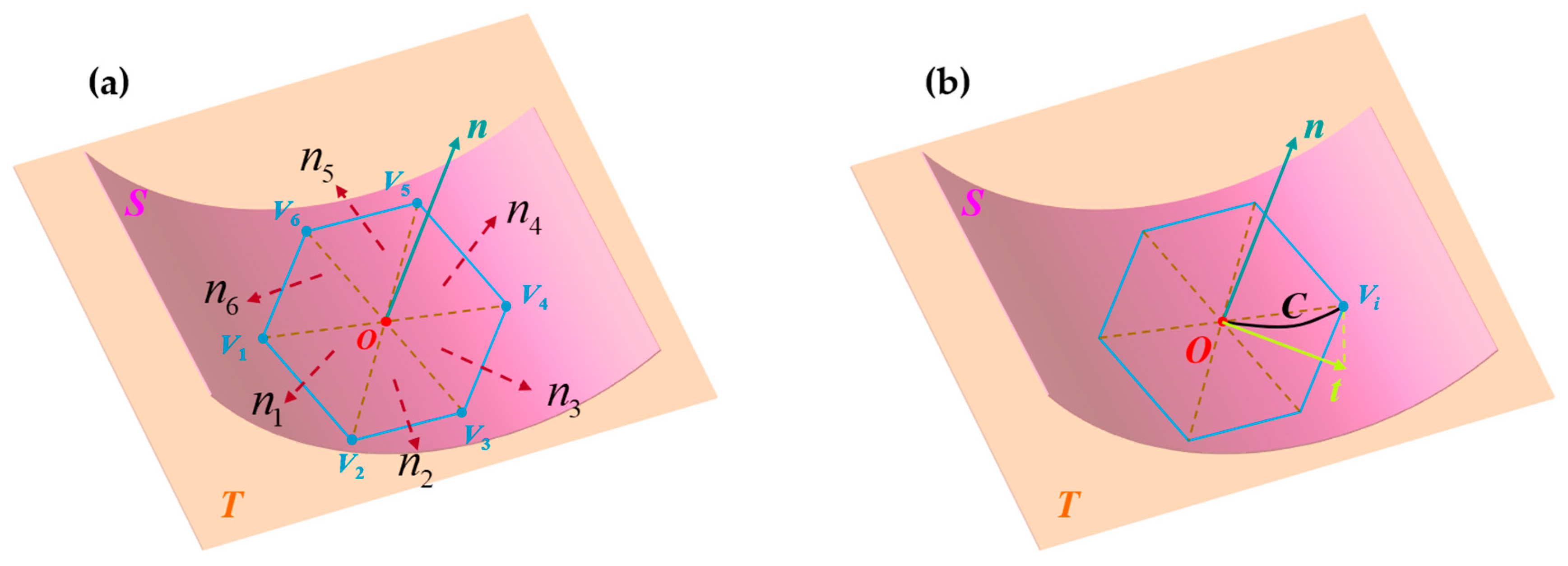
The computation of normal vectors at the vertices of a triangular mesh is a prerequisite for the realization of the curvature computation at the corresponding vertices. As shown in Figure 5a, n_i (i = 1,2,3,4,5,6) are the normal vectors of each triangular mesh, respectively. For any triangular mesh in the mesh surface, the unit normal vector n at the vertex O can be computed by using Equation (11).

$$n={\displaystyle \frac{{\displaystyle \sum _{i=1}^{num}{A}_i{n}_i}}{‖{\displaystyle \sum _{i=1}^{num}{A}_i{n}_i}‖}}$$

(11)

In Equation (11), A_i denotes the area of each triangle mesh.

As shown in Figure 5b, vertices O and V_i belong to a same triangular mesh. Assuming that the expression of the actual curve between point O and point V_i is r = r(C), T is the tangent plane of the surface S at the position of point O, and vector t is the unit tangent vector of OV_i’s projection onto the tangent plane T. Since the vector n has already been computed, t can be obtained by solving Equation (12).

$$t={\displaystyle \frac{O{V}_i-<O{V}_i,n>n}{‖O{V}_i-<O{V}_i,n>n‖}}$$

(12)

For the curve r = r(C), r(0) = O, $r^{\prime }\left(0\right)=t$, $r^{″}\left(0\right)=k_n(t)n$, and k_n(t) is the normal curvature of the point O along the t-direction. Also, $r^{\prime }\left(C\right)$ is always perpendicular to r(C) when the curve r(C) has a fixed length [31]. The curve expression r = r(C) is Taylor-expanded as shown in Equation (13).

$$\begin{array}{c}r(c) =r(0)+r^{\prime }(0)C+{\displaystyle \frac{1}{2!}}{r}^{″}(0)C^2+o(C^3)\\ =O+tC+{\displaystyle \frac{1}{2}}{k}_n(t)n{C}^2+o(C^3)\end{array}$$

(13)

Transforming Equation (13):

$$r(c)-O=tC+{\displaystyle \frac{1}{2}}{k}_n(t)n{C}^2+o(C^3)$$

(14)

Equation (14) can be obtained:

$$\begin{array}{c}n\cdot [r(c)-O]=tC+{\displaystyle \frac{1}{2}}{k}_n(t)n^2{C}^2+o(C^3)\\ ={\displaystyle \frac{1}{2}}{k}_n(t)n^2{C}^2\end{array}$$

(15)

Also, since the inner product of the normal curvature k_n(t) and the tangent line t on the same curve is always 0, Equation (16) can be obtained.

$$[r(c)-O][r(c)-O]=(tC)(tC)+o(C^3)$$

(16)

Simplify Equation (16):

$${\Vert r(c)-O\Vert }^2=C^2+o(C^3)$$

(17)

According to Equations (15) and (17), the equation for k_n(t) is obtained as shown in Equation (18).

$$k_n(t)=\underset{C\to 0}{\lim }{\displaystyle \frac{2n\cdot [r(c)-O]}{{\Vert r(c)-O\Vert }^2}}={\displaystyle \frac{2n\cdot O{V}_i}{{\Vert O{V}_i\Vert }^2}}$$

(18)

The tectonic curvature tensor L is shown in Equation (19).

$$L=k_n(t)(I-n{n}^T)$$

(19)

Solving for the eigenvalues λ₁ and λ₂ of the curvature tensor L, the Gaussian and mean curvatures at the vertex O can be obtained by Equation (20):

$$\left\{\begin{array}{c}{K}_G={\lambda }_1{\lambda }_2\\ H={\displaystyle \frac{{\lambda }_1+{\lambda }_2}{2}}\end{array}\right.$$

(20)

Then, the principal and subsidiary curvatures at vertex O on the mesh surface can be further calculated according to Equation (21).

$$\left\{\begin{array}{c}{k}_1=H+\sqrt{H^2-K_G}\\ k_2=H-\sqrt{H^2-K_G}\end{array}\right.$$

(21)

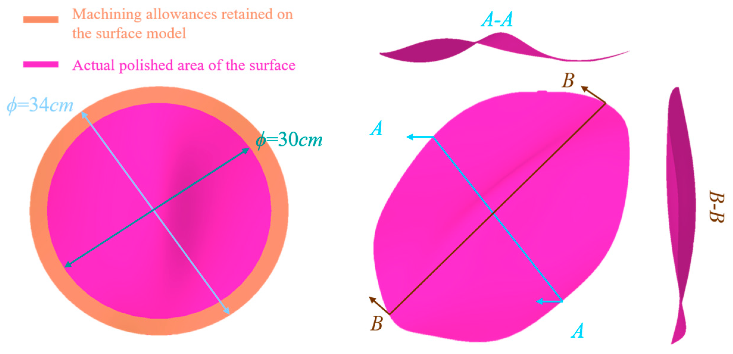
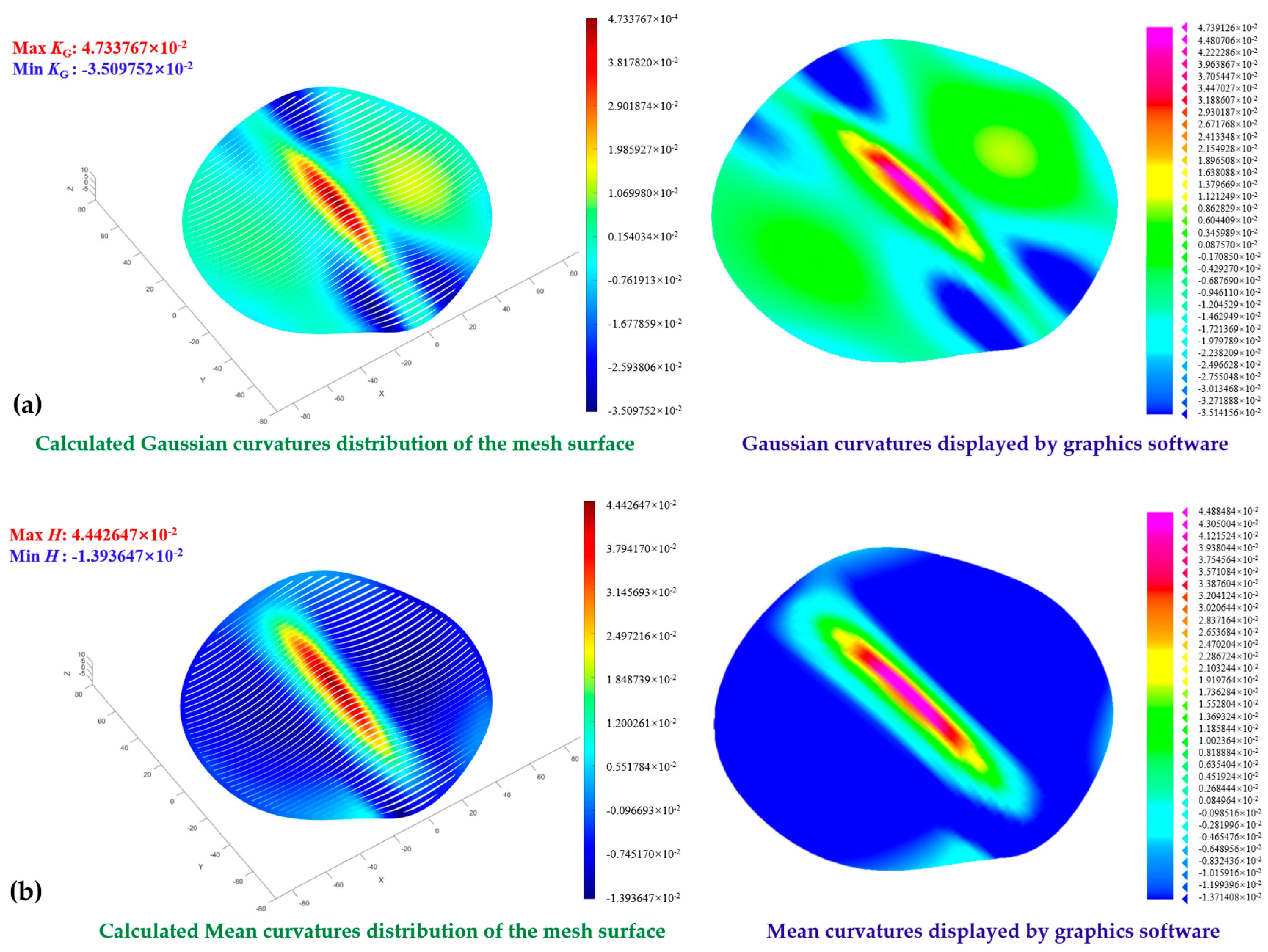
The results of the mesh vertex curvature calculations were verified using the 15 cm × 15 cm equation-free surface shown in Figure 6 (to ensure that the planned polishing trajectory can completely cover the surface, the model retains the machining allowance region during curvature analysis and polishing trajectories generation, as shown in Figure 6). This surface is generated by three random smooth curves through the boundary blending function in the software. Since only Gaussian curvature and mean curvature of the surface can be analyzed in the graphics software, the computed principal and subsidiary curvatures of each vertex on the mesh surface are converted to Gaussian curvature and mean curvature using Equation (20) to compare with the curvature information analyzed in the graphics software, as shown in Figure 7.

As can be seen from the coloring effect in Figure 7, for the equation-free surface shown in Figure 6, the Gaussian curvature and the mean curvature distribution calculated by the algorithm proposed in this paper are consistent with the range of curvature distributions given by the graphics software plotting software. The maximum and minimum values of Gaussian curvature obtained by the mesh point curvature calculation algorithm proposed in this paper are 4.733767 × 10⁻⁴ and −3.509752 × 10⁻⁴, respectively, and the maximum and minimum values of Gaussian curvature of the corresponding surfaces counted by computerized drawing software are 4.739126 × 10⁻⁴ and −3.514156 × 10⁻⁴, respectively. The maximum and minimum mean curvature values obtained by the proposed curvature calculation algorithm are 4.442647 × 10⁻² and −1.393647 × 10⁻², respectively, and the maximum and minimum mean curvature values of the corresponding surfaces calculated by the computerized drawing software are 4.488484 × 10⁻² and −1.371408 × 10⁻², respectively. The maximum error of the Gaussian curvature calculation result is 0.103079%, and the maximum error of the Gaussian curvature calculation result is 0.125322%. The maximum error of the mean curvature calculation result is 1.010212%, and the maximum error of the mean curvature calculation result is 1.621618%.

For any triangular mesh ΔABC, let the coordinates of its three vertices be A(x₁,y₁,z₁), B(x₁,y₂,z₂), and C(x₃,y₃,z₃). Assuming that the principal and subsidiary curvatures computed for each vertex are k_1A, k_2A, k_1B, k_2B, and k_1C, k_2C, respectively. For any trajectory point P(x₀,y₀,z₀) on the triangular mesh, the principal and subsidiary curvatures K_1p and K_2p of point P can be solved by Equation (22).

$$\left\{\begin{array}{c}{K}_{1p}={\tau }_A{k}_{1A}+{\tau }_B{k}_{1B}+{\tau }_C{k}_{1C}\\ K_{2p}={\tau }_A{k}_{2A}+{\tau }_B{k}_{2B}+{\tau }_C{k}_{2C}\end{array}\right.$$

(22)

Assuming that the areas of the sub-triangles formed by point P and the vertices of ΔABC are S_PAB, S_PAC, and S_PBC, and the area of ΔABC is S_ABC. Parameters τ_A, τ_B, and τ_C can be computed by Equation (23).

$$\left\{\begin{array}{c}{\tau }_A={\displaystyle \frac{S_{PBC}}{S_{ABC}}}\\ {\tau }_B={\displaystyle \frac{S_{PAC}}{S_{ABC}}}\\ {\tau }_C={\displaystyle \frac{S_{PAB}}{S_{ABC}}}\end{array}\right.$$

(23)

4. Uniform Coverage Realization of Polishing Trajectory on Mesh Surface

The achievement of uniform coverage in polishing trajectories refers to maintaining a constant overlap of polishing bands generated by any two adjacent polishing trajectories. This condition effectively ensures that there will be no issues of over-polishing or under-polishing during the polishing process.

As shown in Figure 8a, for the planar equidistant polishing trajectory, the amount of overlap between adjacent trajectories is always constant. As shown in Figure 8b, after mapping the planar equidistant polishing trajectories onto a surface, because of the variation in curvature at different positions of the surface, the overlap of the polishing contact areas between adjacent trajectory points cannot be maintained at a constant level, leading to problems of over-polishing and under-polishing.

Therefore, for the realization of uniform coverage of the mapped polishing trajectory, it is first necessary to adjust the position of the point according to the size of the polishing contact area at each trajectory point.

In the actual polishing process, two categories of polishing trajectories are often used. The first is symmetrical trajectories, such as concentric circle trajectories, which have multiple similarly shaped trajectory lines sharing a common trajectory symmetry point. The benefit of employing symmetrical trajectories lies in their capability to achieve comprehensive coverage of the machining surface. The second is asymmetrical trajectories, forming a continuous curve from an origin, which can cover most of the area of the machined surface and effectively guarantee the continuity of the machining process during the machining process. However, the initial region of such trajectories cannot guarantee complete coverage, such as the helical trajectory. In this study, the implementation of algorithms for uniform coverage of a concentric circle trajectory and helical trajectory is discussed separately.

The realization of uniform coverage of polishing trajectories on mesh surfaces involves algorithm design for adjusting the position of any trajectory point on the mesh surface, generation of a seed path, and adjustment of subsequent trajectories.

4.1. Tuning Strategies for Trajectory Points on Mesh Surfaces

The positions of the trajectory points on the mesh surface are adjusted to ensure that the amount of overlap of the polishing bands between arbitrarily neighboring trajectories is always the same. It is assumed that point P_i and point P_j are two polishing trajectory points on a mesh surface, and the radii of the polishing contact areas at points P_i and P_j are a_i and a_j, respectively. Adjust the position of P_j using P_i as the reference point. The target distance A between point P_i and the point P_j is required to satisfy the constraint of Equation (24).

$$A=a_i+a_j-k$$

(24)

In Equation (22), the parameter k denotes the amount of polishing band overlap between two trajectory points. To meet the constraint requirements of Equation (24), the position of point P_j can be adjusted by the following steps.

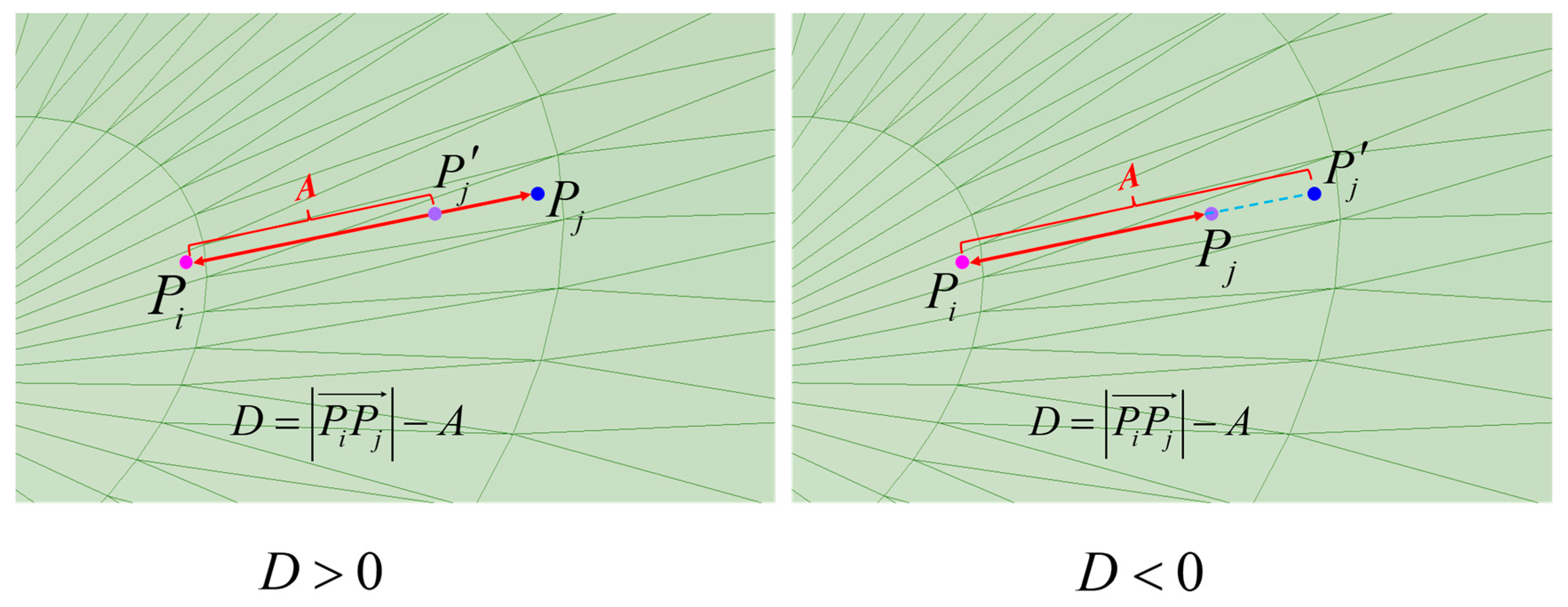
Step 1: Calculate the Euclidean distance $\left|\overrightarrow{P_i{P}_j}\right|$ between point P_i and point P_j. Then, determine the difference $D=\left|\overrightarrow{P_i{P}_j}\right|-A$ between $\left|\overrightarrow{P_i{P}_j}\right|$ and the ideal relation A in Equation (24). As shown in Figure 9, if D > 0, then find a point ${P_j}^{\prime }$ inside the line connecting points P_i and P_j so that $\left|\overrightarrow{P_i{P_j}^{\prime }}\right|=A$. If D < 0, then find a point on the extension of the line connecting points P_i and P_j so that $\left|\overrightarrow{P_i{P_j}^{\prime }}\right|=A$.

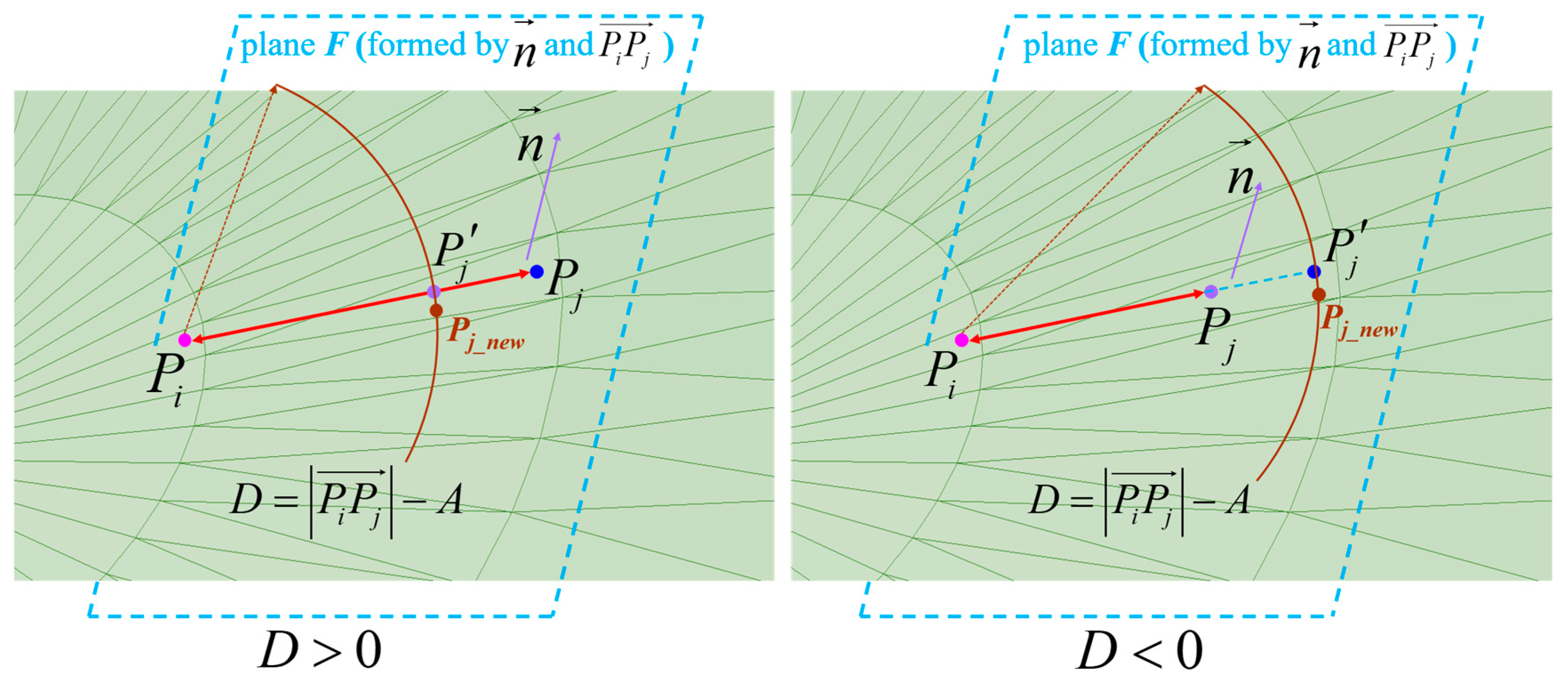
Step 2: As shown in Figure 10, the vector $\overrightarrow{n}$ is the normal vector to the triangular mesh where the point P_j is located, plane F is formed by the vector $\overrightarrow{n}$ and the vector $\overrightarrow{P_i{P}_j}$. A circle is drawn in plane F with the point P_i as its center and the distance value A as its radius. Then, find a point P_{j_new}, which is the intersection of the circle with a certain triangular mesh.

Step 3. Recompute the polishing area radius a_{j_new} at point P_{j_new}, and the Euclidean distance $\left|\overrightarrow{P_i{P}_{j\_new}}\right|$ between point P_{j_new} and the reference point P_i. Evaluate the relationship between $\left|\overrightarrow{P_i{P}_{j\_new}}\right|$ and A according to Equation (24). If $\left|\overrightarrow{P_i{P}_{j\_new}}\right|=A$, then point P_{j_new} is the adjusted trajectory point of point P_j. Otherwise, repeat steps 1 and 2 until the desired point is obtained.

4.2. Seed Path Generation for Concentric Circle Trajectory and Uniform Coverage Implementation

At present, a grating trajectory is mostly used for surface polishing; a grating trajectory is less difficult to realize, but will cause more obvious intermediate frequency error. At the same time, for the rotational symmetry of the surface, a grating trajectory will cause frequent collisions between the polishing tool and the edge of the polished workpiece, resulting in serious edge effects. Therefore, for the rotationally symmetric parts shown in Figure 6, polishing using a spiral or concentric circle trajectory is more stable. The mathematical expression of a concentric circle trajectory in the plane is shown in Equation (25).

$$\left\{\begin{array}{c}x=N\times R\cos \theta +x_c\\ y=N\times R\sin \theta +y_c\end{array}\right.$$

(25)

In Equation (25), N represents the number of circles in the concentric circle, and the radius R denotes both the radius of the initial concentric circle and the spacing between adjacent circles within the concentric circle trajectory. The coordinate (x_c,y_c) is the coordinate of the center point of the concentric circle trajectory on the plane. θ is the rotational angle of each trajectory point relative to the center point. The generation of a concentric circle seed path means adjusting the positions of trajectory points on the initial circle to achieve uniform coverage in the covered region (i.e., trajectories generated in the range of $\theta \in \left[0,2\pi \right]$ during the generation process). This trajectory serves as the foundation for achieving uniform coverage in all subsequent trajectories.

The creation of seed path for concentric circle trajectory entails utilizing the mapped center of concentric circles as a reference point. After adjustment, the Euclidean distance d_i from any trajectory point P_i on the initial concentric circle to the mapped center O′, and the polishing area radius a_i of trajectory point P_i, satisfies the constraint requirements of Equation (26).

$$d_i=\left|\overrightarrow{P_i{O}^{\prime }}\right|=a_i$$

(26)

The process of generating a seed path for a concentric circle trajectory is shown in Figure 11. In Figure 11a, point P_i and point P_j are any two trajectory points on the initial circle of a two-dimensional equidistant concentric circle trajectory (reference trajectory), and the corresponding polishing area radii are a_i1 and a_j1, respectively, and a_i1 = a_j1. When the planar equidistant trajectories are mapped onto the surface mesh, the influence of surface curvature results in changes to both the trajectory shape and the polishing area radius at the trajectory points. As shown in Figure 11b, it is assumed that the radii of the polishing areas at the locations of points P_i and P_j on the reference trajectory are mapped to a surface are a_i2 and a_j2, respectively (a_i2 ≠ a_j2). The Euclidean distance between any mapped trajectory point on the reference trajectory mapped to a surface and the mapped concentric circle center O′ is not exactly equal to the radius of the polishing area at the mapped trajectory point, and the polishing trajectory is no longer able to satisfy the requirement of uniform coverage. Therefore, the position of any trajectory points on the reference trajectory mapped to a surface should be adjusted according to the method provided in Section 4.1. As shown in Figure 11c, it is assumed that the radii of the polishing areas at adjusted points P_i and P_j are ${a_{i2}}^{\prime }$ and ${a_{j2}}^{\prime }$, respectively. The Euclidean distances from points P_i and P_j to the point $O^{\prime }$ are equal to the radii of the polishing area, the new initial concentric circle trajectory not only provides complete coverage of the inner region of the trajectory during the polishing process but also does not cause excessive removal of material, which can be used as a seed path for concentric circle trajectory adjustment on the surface.

The steps for generating a seed path during the realization of uniform coverage of concentric circle polishing trajectory are summarized as follows:

Step 1: Determine the Euclidean distance d_i between each trajectory point on the mapped initial circle of concentric circle trajectory and the mapped center point $O^{\prime }$.

Step 2: Extract the trajectory point p_i whose Euclidean distance from the point $O^{\prime }$ is not equal to a_i (a_i is the radius of the polishing area of the mapped trajectory point on the surface). Determine a plane F_i using the current trajectory point p_i, the mapped center $O^{\prime }$, and the current triangular mesh normal vector n. A circle C_i is generated in the plane F_i with the point $O^{\prime }$ as the center and a_i as the radius. There are multiple intersections of the circle C_i with the triangular mesh, and the intersection p_{i_new} with the closest distance to the point p_i is extracted.

Step 3: Determine the polishing area’s radius a_{i_new} of point p_{i_new}, and calculate the Euclidean distance d_{i_new} between the point p_{i_new} and the center $O^{\prime }$ of the mapped concentric circle polishing trajectory. Determine whether the relationship between a_{i_new} and d_{i_new} satisfies the constraint requirements of Equation (26). If satisfied, the point p_{i_new} is the desired optimized trajectory point. Otherwise, continue the iterative process of step 2 retrieval.

After all trajectory points on the initial concentric circle trajectory have been adjusted by the above steps, a seed path can be obtained, which is the initial datum for subsequent concentric circle polishing trajectory adjustments.

The optimization and adjustment strategies for subsequent concentric circle trajectories are as follows:

Step 1: It is assumed that there are M trajectory points on the seed path T₁, and N trajectory points on the second mapped concentric circle trajectory T₂. Solve for the Euclidean distance between each trajectory point on the trajectory T₂ and each trajectory point on the seed path T₁. For each trajectory point P_2,i on the trajectory T₂, there will be a trajectory point P_1,j with the closest Euclidean distance on the seed path T₁;

Step 2: Calculate the polishing area radius a_1,j at point P_1,j, the polishing area radius a_2,i at point P_2,i, and the Euclidean distance $\left|\overrightarrow{P_{1,j}{P}_{2,i}}\right|$ between points P_1,j and P_2,i. Then, calculate the difference between $a_{2,i}+a_{1,j}-k$ and $\left|\overrightarrow{P_{1,j}{P}_{2,i}}\right|$ (Here, k represents the overlap between two adjacent polishing bands, which is a predetermined value). If the Euclidean distance $\left|\overrightarrow{P_{1,j}{P}_{2,i}}\right|$ is not equal to $a_{2,i}+a_{1,j}-k$, the points P_2,i are repositioned according to the method provided in Section 4.1 until the radius ${a_{2,j}}^{\prime }$ of the retrieved polishing area at point P_{2,i_new,} and the Euclidean distance $\left|\overrightarrow{P_{1,j}{P}_{2,i\_new}}\right|$ between point P_{2,i_new} and point P_1,j exactly satisfy the relation of $a_{1,j}+{a_{2,j}}^{\prime }-k=\left|\overrightarrow{P_{1,j}{P}_{2,i\_new}}\right|$.

Step 3: Using the adjusted second circle of the concentric circle trajectory as the new seed path, adjust the third circle according to the strategy described in steps 1 to 2, until the remaining circular trajectories are optimized. The flowchart of the uniform coverage trajectory planning algorithm for concentric circle polishing trajectories is shown in Figure 12.

By the above algorithmic principles, the uniform coverage of concentric circle polishing trajectory is simulated of the equation-free surface shown in Figure 6. The polishing process parameters used in the simulation are shown in

Table 1. Parameters for simulation of uniform coverage of polishing trajectories.

Name	Value
Polishing load (Q)	15 N
Polishing tool radius (R1)	38 mm
Elastic modulus of polishing tool (E1)	38.29 Mpa
Elastic modulus of the polished part (E2)	193,000 Mpa
Polishing tool’s Poisson’s ratio (μ1)	0.3
Poisson’s ratio of the polished part (μ2)	0.33

. The simulation results are shown in Figure 13.

4.3. Seed Path Generation for Helical Trajectory and Uniform Coverage Implementation

The mathematical expression of an equally spaced helical trajectory in a two-dimensional plane is shown in Equation (27).

$$\left\{\begin{array}{c}x=(h_a+h_b\theta )\cos \theta +x_c\\ y=(h_a+h_b\theta )\sin \theta +y_c\end{array}\right.$$

(27)

In Equation (27), parameters h_a and h_b are the initial radius and the spacing value of the equally spaced helix, respectively. θ is the rotational angle of each trajectory point relative to the starting point of the helical trajectory. The coordinates (x_c,y_c) are the starting points of the helical trajectory in the plane. The seed path generation based on the helical trajectory is only for trajectory points generated within the range of $\theta \in \left[0,2\pi \right]$.

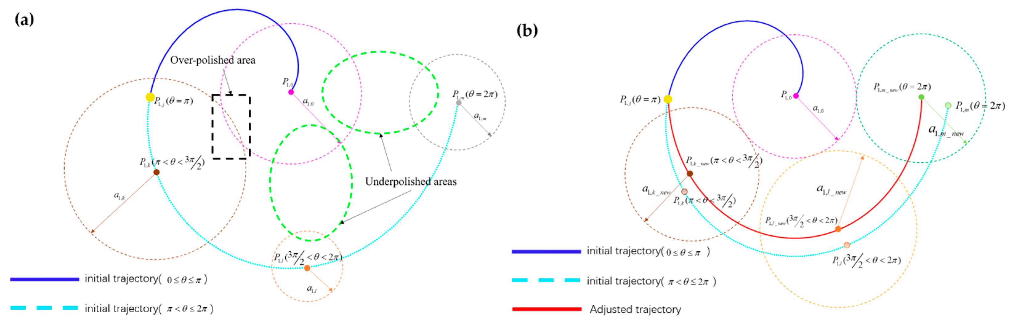
From the mathematical properties of the helical trajectory, it can be seen that the helical trajectory belongs to an unclosed curve. As shown in Figure 14a, for the helical trajectory in the range of $\theta \in \left[\pi ,2\pi \right]$, there is a defect that does not completely cover the polishing area. To enhance the coverage of helical trajectory within the range of $\theta \in \left[\pi ,2\pi \right]$, adjustments are made to the helical trajectory points within the range of $\theta \in \left[\pi ,2\pi \right]$. As shown in Figure 14a, point P_1,0 is the first trajectory point on the trajectory, point P_1,j is the trajectory point with θ value equal to π, point P_1,k is the trajectory point with θ value in the range of $\left(\pi ,{\displaystyle \raisebox{1ex}{$3\pi $}\!\left/ \!\raisebox{-1ex}{$2$}\right.}\right)$, point P_1,l is the trajectory point with θ value in the range of $\left({\displaystyle \raisebox{1ex}{$3\pi $}\!\left/ \!\raisebox{-1ex}{$2$}\right.},2\pi \right)$, and point P_1,m is the trajectory point with θ value equal to 2π. Parameters a_1,j, a_1,k, a_1,l, and a_1,m are the radii of the polishing areas of the above points on the mesh surface, respectively. In this case, due to the different radius of the polishing area at each trajectory point, the over-polished or under-polished region is generated between point P_1,k, point P_1,l, point P_1,m and point P_1,0.

By adjusting the position of any point P_1,i (e.g., point P_1,j, P_1,k, P_1,l, and P_1,m in Figure 14a) in the range of $\theta \in \left[\pi ,2\pi \right]$, a new trajectory point P_{1,i_new} (e.g., point P_{1,j_new}, P_{1,k_new}, P_{1,l_new}, and P_{1,m_new} in Figure 14b) can be obtained. The Euclidean distance between the trajectory point P_{1,i_new} and the trajectory point P_1,0(x_c,y_c) satisfies the constraints in Equation (28). In this case, the final seed path obtained has a regular helical trajectory in the first half and a half-circle trajectory in the second half.

$$d_{1,i}=\left|\overrightarrow{P_{1,i\_new}{P}_{1,0}}\right|=a_{1,i\_new}+a_{1,0}-k$$

(28)

In Equation (28), a_{1,i_new} and a_1,0 represent the radius of the polishing area of the trajectory point P_{1,i_new} and P_1,0, respectively.

Combining the trajectory point position adjustment measures in Section 4.1 and the previously mentioned seed path generation strategy for a helical trajectory, the positions of the helical trajectory points in the range of $\theta \in \left[\pi ,2\pi \right]$ are adjusted, and the final seed path effect obtained is shown as the red trajectory in Figure 14b. From Figure 14b, it can be seen that the trajectory points in the range of $\theta \in \left[0,\pi \right]$ are still in the form of a conventional helix, while the trajectory points in the range of $\theta \in (\pi ,2\pi ]$ are adjusted to be consistent with the distribution of trajectory points on a circular trajectory. The adjusted seed path of the helical trajectory ensures consistent material removal and effectively increases polishing coverage within the seed path.

Similar to the process of realizing uniform coverage of a concentric circle trajectory, the obtained seed path of the helical trajectory is used as the initial reference for the adjustment of subsequent polishing trajectories. The corresponding adjustment steps are summarized as follows:

Step 1: As shown in Equation (27), each 2π increase in the angular value θ is considered to generate a new helical trajectory. At the same time, the number of trajectory points contained in each helical trajectory is equal. Due to the continuous nature of the helical trajectory, a point-by-point optimization strategy is used to optimally adjust the position of each point on the subsequent helical trajectory. For any trajectory point P_2,i on the second helical trajectory T₂, a point P_1,i can be found on the seed path T₁, and the difference in phase angle between these two points is 2π.

Step 2: Calculate the polishing area radius a_1,i at point P_1,i, the polishing area radius a_2,i at point P_2,i, and the Euclidean distance values $\left|\overrightarrow{P_{1,i}{P}_{2,j}}\right|$ between points P_1,i and P_2,i. Determine the relationship between the difference of $\left|\overrightarrow{P_{1,i}{P}_{2,j}}\right|$ and $a_{2,i}+a_{1,i}-k$. (k represents the overlap between two adjacent polishing bands, which is a predetermined value.) If $\left|\overrightarrow{P_{1,i}{P}_{2,i}}\right|\ne a_{2,i}+a_{1,i}-k$, the position of the trajectory point P_2,i is adjusted according to the method provided in Section 4.1, until the new radius ${a_{2,i}}^{\prime }$ of the polishing area at the adjusted position of point P_2,j and the Euclidean distance $\left|\overrightarrow{P_{1,i}{P}_{2,i}}\right|$ satisfy the constraint $\left|\overrightarrow{P_{1,i}{P}_{2,i}}\right|={a_{2,i}}^{\prime }+a_{1,i}-k$.

Step 3: Using the adjusted second helical trajectory as the new seed path, the third trajectory is optimized according to the strategy described in steps 1–2. Using the same method, the optimization of all helical polishing trajectories can be completed.

In the corresponding trajectory optimization process, the adjustment reference for the first trajectory point of each helix is the first trajectory point of the previous helix, and the adjustment reference for the last trajectory point of each helix is the last trajectory point of the previous helix. This results in a clear break between the last trajectory point of the ith helical trajectory and the first trajectory point of the i+1th helical trajectory, as shown in Figure 15a.

To realize the smooth connection between two adjacent helical trajectories, a smooth connection algorithm for helical trajectories based on a cubic interpolation strategy is proposes. Assuming that each helical trajectory has N trajectory points, the last n trajectory points of the ith helix and the first n trajectory points of the i + 1th helix are extracted. (In this paper, n = 4.) As shown in Figure 15b, points A₁–A₄ represent extraction points of the ith trajectory, and points B₁–B₄ represent extraction points of the i + 1th trajectory.). The average values of X and Y coordinates between these n sets of trajectory points are solved by Equation (29).

$$\left\{\begin{array}{c}{p}_{av,1}=\left(x_{av,1},y_{av,1}\right)\left({\displaystyle \frac{x_{i,N-n+1}+x_{i+1,1}}{2}},{\displaystyle \frac{y_{i,N-n+1}+y_{i+1,1}}{2}}\right)\\ ⋮\\ p_{av,n}=\left(x_{av,n},y_{av,n}\right)=\left({\displaystyle \frac{x_{i,N}+x_{i+n,n}}{2}},{\displaystyle \frac{y_{i,N}+y_{i+1,n}}{2}}\right)\end{array}\right.$$

(29)

Extract the X and Y coordinates of the N-nth trajectory point of the ith helical trajectory and the X and Y coordinates of the n + 1th trajectory point of the i + 1th helical trajectory (denoted as (x_i,N−n, y_i,N−n) and (x_i+1,n+1, y_i+1,n+1)). Combine these coordinate values with the calculated result of Equation (29) and substitute the coordinates of the selected points into the cubic interpolation Equation (30) to obtain a smooth trajectory curve.

$$\left\{\begin{array}{c}{y}_{i,N-n}=S_{i,N-n}(x)=a+b\left(x-x_{i,N-n}\right)+c{\left(x-x_{i,N-n}\right)}^2+d{\left(x-x_{i,N-n}\right)}^3\\ y_{av,1}=S_{av,1}(x)=a+b\left(x-x_{av,1}\right)+c{\left(x-x_{av,1}\right)}^2+d{\left(x-x_{av,1}\right)}^3\\ ⋮\\ y_{i+1,n+1}=S_{i+1,n}(x)=a+b\left(x-x_{i+1,n}\right)+c{\left(x-x_{i+1,n}\right)}^2+d{\left(x-x_{i+1,n}\right)}^3\end{array}\right.$$

(30)

The key to segmented cubic interpolation is to ensure that both the function values and derivatives of the interpolated curves at the nodes are continuous, so the cubic interpolation Equation (30) also has the following two characteristics: (1) the first-order derivatives of the cubic interpolation Equation (30) are continuous; (2) the second-order derivatives of the cubic interpolation Equation (30) are continuous. Therefore, the constraints described in Equation (31) are introduced based on the cubic interpolation Equation (30).

$$\left\{\begin{array}{c}{S_{i,N-n}}^{\prime }(x_{av,1})={S_{av,1}}^{\prime }(x_{av,1})\\ {S_{av,1}}^{\prime }(x_{av,2})={S_{av,2}}^{\prime }(x_{av,2})\\ ⋮\\ {S_{av,n}}^{\prime }(x_{i+1,n})={S_{i+1,n}}^{\prime }(x_{i+1,n})\\ {S_{i,N-n}}^{″}(x_{av,1})={S_{av,1}}^{″}(x_{av,1})\\ {S_{av,1}}^{″}(x_{av,2})={S_{av,2}}^{″}(x_{av,2})\\ ⋮\\ {S_{av,n}}^{″}(x_{i+1,n})={S_{i+1,n}}^{″}(x_{i+1,n})\\ {S_{i,N-n}}^{″}(x_{i,N-n})=0\\ {S_{i+1,n}}^{″}(x_{i+1,n})=0\end{array}\right.$$

(31)

The smooth connection between two adjacent helical trajectories can be realized by associating Equations (29)–(31). The results of the neighboring trajectories smoothing process are shown in Figure 15c, mapping all the smoothed planar trajectory points to the surface to obtain a smooth helical polishing trajectory on the surface.

The flowchart of the uniform coverage trajectory planning algorithm for concentric circle polishing trajectories is shown in Figure 16.

Still using the polishing process parameters shown in Table 1, the uniform coverage of the helical polishing trajectory is simulated on the equation-free surface shown in Figure 6. The simulation results are shown in Figure 17.

5. Experimental Tests of Uniform Coverage of Polishing Trajectories on an Equation-Free Surface

5.1. Materials and Methods

In order to verify the effectiveness of the polishing trajectory uniform coverage algorithm proposed in this paper, two surfaces were machined according to the surface model shown in Figure 6 for polishing comparison experiments (workpiece material: 304 stainless steel, elastic modulus: approximately 193,000 Mpa, Poisson’s ratio: approximately 0.33). In this case, for the polishing of workpiece 1, the helical uniformly covering polishing trajectory from Figure 17a is employed. As shown in Figure 18a, a helical non-uniform coverage polishing trajectory was obtained for the polishing of workpiece 2 using the surface parameterization trajectory generation method proposed in reference [28]. Before the polishing experiments began, the trajectory points of these two trajectories were culled to ensure that the arc length (step length) between each of the two consecutive trajectory points remained constantly (C = 0.5 mm). This approach was adopted to prevent damage to the surface shape that could potentially arise from the use of overly dense trajectory points during the polishing process.

During the polishing process, each workpiece was subjected to six rounds of polishing, using diamond abrasives of 28 µm, 20 µm, and 15 µm in order, and replacing the diamond abrasives after every two rounds of the polishing process. In addition, during the experimental process, every time the diamond abrasive was replaced, the planar helical was rotated by 120° around the Z-axis, and then a new polishing trajectory was generated. The polishing tool orientation angle ψ (the angle between the tool axis and the normal vector at the trajectory point), the tool rotation speed ω, and the tool feed rate v_a were all maintained constant. The polishing equipment utilized an ABB IRB6700 industrial robot (ABB; Zurich, Switzerland; maximum payload: 200 kg, repetitive positioning accuracy: 0.05 mm), and a spherical rubber polishing head was employed as the polishing tool, with a polyurethane polishing pad affixed to its outermost layer, as illustrated in Figure 19a. A force control unit (model: xPush500; manufacturer: xBang; Shenzhen, China; maximum load: 48 N, stroke: ±10 mm, computational frequency: 10 kHz, system response frequency: 1 kHz) was integrated between the robot end-effector and the polishing tool to ensure a constant polishing load. For post-polishing quality assessment, the surface roughness (Sa value) and PV (Peak-to-Valley) values were measured using a white light interferometer (Sensofar S neox 035; Sensofar; Terrassa, Spain; X/Y-axis accuracy: 0.18 µm, Z-axis precision: 0.1 nm, Figure 19b) and a contact profilometer (Taylor Hobson PGI 1240; Taylor Hobson; Leicester, UK; vertical resolution: 0.8 nm, Figure 19c), respectively. The complete set of process parameters used during polishing is summarized in

Table 2. Parameters for polishing experiments of different polishing trajectories.

Name	Value	Name	Value
Polishing load (Q)	15 N	Tool orientation angle (ψ)	20°
Polishing tool radius(R1)	38 mm	Diamond abrasives (µm)	28→20→15
Elastic modulus of polishing tool (E1)	38.29 Mpa	Elastic modulus of workpieces (E2)	193,000 Mpa
Polishing tool’s Poisson’s ratio (μ1)	0.3	Poisson’s ratio of the workpieces (μ2)	0.33
Tool rotation rate (ω)	600 r/min	Tool feed speed (va)	60 mm/min
Workpiece 1 trajectory length	4228.3827 mm	Workpiece 2 trajectory length	4284.8328 mm
Polishing duration for workpiece 1	70.47 min per round	Single polishing time for workpiece 2	71.41 min per round

.

5.2. Experimental Results Statistics and Discussion

The initial state and the effects after polishing of the two workpieces are shown in Figure 20.

As shown in Figure 20, both workpieces were polished to a mirror finish. To deeply analyze the difference in surface quality of the two workpieces after polishing, five paths are selected in different directions on the surface of the workpiece as shown in Figure 21, and each path is divided into five inspection areas for measurement.

The results of roughness inspection in each inspection area of workpiece 1 and workpiece 2 are shown in Figure 22.

From Figure 22a, the maximum value of roughness after polishing of workpiece 1 is 9.91352 nm, and the minimum value is 9.17118 nm. From Figure 22b, the maximum value of roughness after polishing of workpiece 2 is 14.4527 nm, and the minimum value is 12.5009 nm. To summarize, workpiece 1 has a lower roughness after polishing and the roughness is more consistent across the different inspection areas.

Due to the large fluctuation of the Z-coordinate of each inspection area, the PV value of each inspection area is detected individually, and the inspection results are ordered in series according to the inspection paths to which they belong to obtain the PV value on each inspection path, as shown in Figure 23.

From Figure 23a, the maximum value of PV after polishing of workpiece 2 is 176.6296 nm, and the minimum value is 167.7444 nm. From Figure 23b, the maximum value of PV after polishing of workpiece 2 is 480.2178 nm, and the minimum value is 456.2963 nm. To summarize, workpiece 2 has a lower PV value after polishing and the PV values are more consistent across the different inspection paths.

In order to further illustrate the difference in the surface quality of the two workpieces after polishing, the roughness and PV values of each inspection area before and after polishing on different inspection paths were inspected five times, and the maximum value of each inspection result was extracted and the average value was calculated, and the statistical results are shown in

Table 3. Mean values of Sa and PV of each inspection area after polishing of the workpieces on path 1.

Area	Workpiece 1				Workpiece 2
	Sa (nm)		PV (nm)		Sa (nm)		PV (nm)
	Unpolished	Polished	Unpolished	Polished	Unpolished	Polished	Unpolished	Polished
area1	582.5014	9.5056	4426.1587	173.2557	543.8643	14.1047	4378.8038	455.7085
area 2	425.4671	9.1245	4445.3286	187.5659	423.6097	13.6572	4276.9171	487.2933
area 3	425.5196	9.6356	3258.8054	172.5252	430.4128	13.4394	3357.1529	485.1796
area 4	489.2731	9.8154	2869.7224	185.4595	464.4385	14.2867	2936.7531	468.7652
area 5	366.3039	9.6156	2003.4659	173.4269	401.8265	14.4715	2179.3737	470.4927

,

Table 4. Mean values of Sa and PV of each inspection area after polishing of the workpieces on path 2.

Area	Workpiece 1				Workpiece 2
	Sa (nm)		PV (nm)		Sa (nm)		PV (nm)
	Unpolished	Polished	Unpolished	Polished	Unpolished	Polished	Unpolished	Polished
area1	528.8442	9.4565	3454.8557	176.7272	527.6154	13.6571	3846.5587	489.8363
area 2	419.5358	9.6436	4122.7031	179.4512	422.6265	12.8653	3752.7363	467.3256
area 3	367.1066	9.2048	2711.1598	188.9689	386.9353	12.8758	2594.6278	472.3278
area 4	491.8922	9.9254	3125.2045	163.7154	461.2387	13.1582	2975.5875	476.5586
area 5	455.7371	9.1154	2124.7252	178.2265	434.6866	13.8876	2112.2147	474.1983

,

Table 5. Mean values of Sa and PV of each inspection area after polishing of the workpieces on path 3.

Area	Workpiece 1				Workpiece 2
	Sa (nm)		PV (nm)		Sa (nm)		PV (nm)
	Unpolished	Polished	Unpolished	Polished	Unpolished	Polished	Unpolished	Polished
area1	509.3008	9.1468	3034.1795	171.2334	533.2156	13.8079	3972.2125	463.6007
area 2	431.1691	9.4214	2088.9117	180.1667	448.2562	12.9172	2341.3088	484.4595
area 3	307.1746	9.4657	2095.7358	182.8459	310.6255	13.1307	2074.3562	466.7262
area 4	365.5206	9.7376	2069.8452	165.6077	347.3845	13.5024	2132.1285	476.9021
area 5	431.5875	9.4156	3059.4086	160.5217	417.9562	13.1258	2984.2144	465.9196

,

Table 6. Mean values of Sa and PV of each inspection area after polishing of the workpieces on path 4.

Area	Workpiece 1				Workpiece 2
	Sa (nm)		PV (nm)		Sa (nm)		PV (nm)
	Unpolished	Polished	Unpolished	Polished	Unpolished	Polished	Unpolished	Polished
area1	591.4441	9.5565	3022.3643	194.1235	550.7481	13.7582	3111.9055	455.9252
area 2	497.1372	9.7263	2054.6957	174.1452	453.3145	12.8021	2217.3739	481.9202
area 3	333.9049	9.6251	2013.8964	167.4478	320.6787	13.5254	2089.4589	462.6542
area 4	428.4521	9.4025	2014.9234	176.1485	406.5006	13.2586	2074.6624	473.5586
area 5	484.3079	9.3151	3075.1365	160.7156	453.2658	12.5731	2879.4013	452.2534

and

Table 7. Mean values of Sa and PV of each inspection area after polishing of the workpieces on path 5.

Area	Workpiece 1				Workpiece 2
	Sa (nm)		PV (nm)		Sa (nm)		PV (nm)
	Unpolished	Polished	Unpolished	Polished	Unpolished	Polished	Unpolished	Polished
area1	583.1179	9.8595	3025.5071	153.3179	592.7071	13.3513	3262.1743	465.3099
area 2	469.7194	9.2326	2813.4352	186.9067	457.3154	12.5266	2520.7791	484.6853
area 3	486.7082	9.5641	2243.3976	187.5711	427.7963	13.2753	2132.7937	455.6573
area 4	435.7357	9.5595	2928.2881	174.6362	423.9273	12.8951	2787.3019	461.3927
area 5	451.5751	9.5807	3050.5776	175.7797	455.9018	12.9861	3115.5241	475.4601

.

As observed in Table 3, Table 4, Table 5, Table 6 and Table 7, workpiece 1 exhibited superior surface roughness (Sa) and PV values after polishing compared to workpiece 2, with the distributions of both roughness and PV values demonstrating greater consistency. This improvement can be attributed to the following factors:

• Unlike the parameterization trajectory generation method, the mapping method employed for trajectory generation is unaffected by mesh distortion. Consequently, the generated trajectories conform more accurately to the actual surface geometry;
• The trajectories, characterized by uniform coverage capability, effectively mitigate both over-polishing and under-polishing during the process. This leads to a significant enhancement in the consistency of material removal.

In summary, under identical polishing parameters and within the same polishing cycle duration, trajectories possessing uniform coverage capability ensure more stable and consistent surface polishing quality.

6. Conclusions

This paper has presented a comprehensive study on the generation and optimization of polishing trajectories for equation-free surfaces, specifically targeting the challenges of sub-aperture polishing with compliant spherical tools, and the following conclusions are obtained:

• Direct Mesh-Based Trajectory Generation: A novel trajectory mapping method operating directly on the surface mesh model was proposed. This method effectively bypasses the need for solving complex surface equations, significantly reducing the difficulty and computational burden associated with generating precise polishing paths for complex freeform optical surfaces lacking closed-form mathematical descriptions;
• Accurate Curvature Solution on Mesh: An algorithm for accurately computing sur-face curvature at polishing trajectory points directly on the mesh was developed. By leveraging vertex curvatures and local fitting, this method provides the high-fidelity curvature data essential for calculating the polishing tool contact area—also a critical input for modeling material removal. This accuracy is vital for predictable outcomes on surfaces with significant curvature variations or discontinuities;
• Uniform Coverage Optimization Algorithm: An algorithm was introduced to achieve uniform coverage of polishing trajectories across the mesh surface. By dynamically adjusting trajectory point positions, this algorithm ensures consistent overlap between adjacent paths, precisely matching predetermined values. This method effectively avoids over-polishing and under-polishing (especially critical for minimizing high-spatial frequency error), and accelerates convergence towards the desired surface finish within the same processing time;
• Experimental Validation: The significant impact of uniform coverage on final polishing quality was experimentally verified. Results demonstrate that trajectories optimized for uniform coverage yield measurably superior surface quality compared to non-uniform paths. Critically, a substantial reduction in High-Spatial Frequency (HSF) errors (quantified using Sa) was observed, directly addressing a key quality challenge in precision optical finishing;
• Broad Applicability: While specifically designed for equation-free surfaces, the proposed algorithms are equally applicable to surfaces with known equations by first converting them into mesh representations. This extends the utility of the methods to a wide spectrum of optical manufacturing tasks requiring deterministic sub-aperture polishing, including traditional aspheric optics and complex hybrid surfaces.

At the same time, the methodologies developed in this research are particularly impactful for the manufacturing and finishing of advanced optical components where traditional trajectory planning struggles:

• Complex Freeform Optics: Enables efficient and high-quality deterministic polishing of intricate freeform surfaces used in next-generation imaging systems (e.g., head-mounted displays for AR/VR), illumination optics, and advanced laser systems, where surface descriptions are often purely geometric (mesh-based);
• Rapid Prototyping and Mold Making: Provides a robust solution for polishing complex optical molds (e.g., for injection molding or glass pressing) directly from scanned or designed mesh data, accelerating the mold development cycle and improving mold surface quality, directly impacting the quality and yield of molded optics.

By directly addressing the challenges of trajectory generation, curvature accuracy, and uniform coverage on complex mesh-defined surfaces, this work provides practical and effective algorithms that enhance the capability and efficiency of sub-aperture polishing processes.