Abstract
This study focuses on a blood pump system equipped with four radial active magnetic bearings (RAMBs). The finite element method (FEM) was employed to optimize the physical parameters of the system. Based on this optimization, two intelligent PID tuning strategies—particle swarm optimization (PSO) and backpropagation (BP) neural networks—were compared. First, a differential control model of a single-degree-of-freedom active magnetic bearing was developed, based on the topology and operating principles of the radial magnetic bearings. Then, magnetic circuit parameters were precisely identified through finite element simulation, enabling accurate optimization of the physical model. To enhance control accuracy, intelligent tuning strategies based on PSO and BP neural networks were applied, effectively addressing the limitations of conventional PID controllers, which often rely on empirical tuning and lack precision. Finally, simulation experiments were conducted to evaluate the optimization performance of PSO and BP neural networks in the magnetic bearing control system. The results demonstrate that the improved PSO algorithm offers significant advantages over both the BP neural network and traditional manual PID tuning. Specifically, it achieved a rise time of 0.0049 s, a settling time of 0.0079 s, and a steady-state error of 0.0013 mm. The improved PSO algorithm ensures system stability while delivering faster dynamic response and superior control accuracy.
1. Introduction
The long-term operational stability of rotary blood pumps is a key performance parameter that determines their clinical applicability. Numerous clinical studies have shown that continuous friction and wear at the rotor–stator contact interface of traditional mechanical bearings is the primary cause of performance degradation and failure in blood pumps [1,2]. The third-generation blood pumps, based on magnetic suspension technology, fundamentally overcome this technical bottleneck by achieving contactless support [3,4]. Magnetic bearings can be classified, based on their suspension principle, into permanent magnetic bearings (PMBs), active magnetic bearings (AMBs), and hybrid magnetic bearings (HMBs) [5,6,7]. A purely PMB-based system, in which all six degrees of freedom (DOFs) of a rigid body are supported solely by PMBs, is physically unfeasible. According to Earnshaw’s theorem [8], at least one unstable DOF always exists. In practice, these unstable DOFs can be stabilized by introducing additional forces from other physical mechanisms, such as active electromagnets, superconducting magnets, diamagnetic materials, or gyroscopic effects. The suspension performance of PMBs depends solely on their structural parameters and lacks active regulation capability. In contrast, AMBs can enhance suspension precision and system stability [9], but they require continuous power supply to maintain rotor levitation, leading to increased power consumption and excessive temperature rise. To address this issue, hybrid magnetic bearing systems combining permanent magnets and electromagnets (HMBs) have been increasingly adopted in the design of artificial heart pumps in recent years [10,11].
Since the rotor system supported by HMBs forms an open-loop unstable system [12], feedback control must be implemented to maintain system equilibrium after determining the structural parameters of the HMB [13,14]. Consequently, the design of a feedback controller is an essential component of magnetic bearing systems. Among various approaches, the proportional–integral–derivative (PID) control method remains widely used for magnetic bearing feedback control due to its broad applicability, simple structure, and ease of tuning [15,16,17]. However, as requirements for precision and stability of magnetic bearing systems increase [18], there is a growing demand for enhanced control performance. Numerous researchers have proposed improvements to the traditional PID control approach. For instance, Hutterer et al. [19] used the linear quadratic regulator (LQR) method to optimize the PID controller for system stability; Chen et al. [20] proposed a high-precision position control strategy for AMB-based high-speed flywheel rotor systems using an inverse system method and an extended two-degree-of-freedom (2DOF) PID controller; Gupta et al. [21] employed algorithm-driven intelligent PID controller optimization for AMB control. These studies collectively demonstrate the wide application of PID control in the magnetic bearing field, and its enhanced performance when optimized with intelligent algorithms. Recently, some scholars have also adopted machine learning and other artificial intelligence (AI) methods to optimize control systems, achieving certain positive outcomes [22].
This study focuses on a hybrid magnetic bearing system equipped with four RAMBs. The model and structure of the system are introduced, and a single-degree-of-freedom differential control model is derived based on the principle of virtual work and magnetic circuit analysis. The model parameters are further refined using finite element analysis. Building upon the corrected parameters, two popular PID intelligent optimization algorithms—PSO and BP neural networks—are applied. Finally, simulation-based performance comparisons of the system are presented and analyzed.
2. Magnetic Bearing System Model and Structure
2.1. Structure of the Blood Pump and Magnetic Bearings
The Figure 1 below shows the structural schematic diagram of a blood pump.The blood pump described in this study adopts a radially active control scheme with passive axial suspension. Magnetic fields generated by four peripheral electromagnetic coils levitate the entire rotor and actively regulate its radial displacement to maintain central stability. Axial tilt is passively controlled by the magnetic fields produced by the interaction between the four coils and the permanent magnets embedded in the rotor.
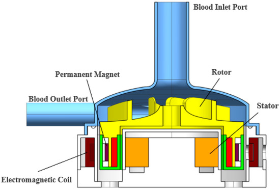
Figure 1.
Cross-sectional view of the magnetically levitated blood pump.
As shown in Figure 2, the magnetic bearing structure used in this study is a hybrid magnetic bearing (HMB) equipped with four RAMBs. Compared to active magnetic bearings (AMBs), the permanent magnets in HMBs provide a bias magnetic field that generates part of the suspension force, thereby reducing the power demand of the magnetic bearings in the blood pump. In addition, the bias magnetic field, together with the damping effect introduced by the fluid environment of the pump, enhances the stability of the control system. Unlike pure permanent magnetic bearings (PMBs), HMBs allow active adjustment of the rotor’s radial position, which is essential for dynamic control.
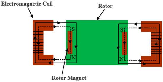
Figure 2.
Cross-sectional view of the magnetic bearing in the blood pump.
2.2. Magnetic Bearing System Model
In electromagnetic bearing systems, it is typically assumed that the magnetic flux is entirely confined within the ferromagnetic core (i.e., there is negligible leakage flux) for magnetic field calculations. Given the much higher magnetic permeability of the core compared to air, and the fact that magnetic field lines pass almost perpendicularly through the core, static field analysis can be extended to discontinuous field conditions. In this study, an analytical approach is used to derive the magnetic force expression for a single-degree-of-freedom magnetic bearing under the following simplifying assumptions:
- The magnetic flux Φ is entirely concentrated within the core magnetic circuit;
- The cross-sectional area of the core Afe is equal to and constant with that of the air gap A;
- The magnetic field is uniformly distributed along both the core length lfe and the air gap length 2s.
2.2.1. Magnetic Circuit
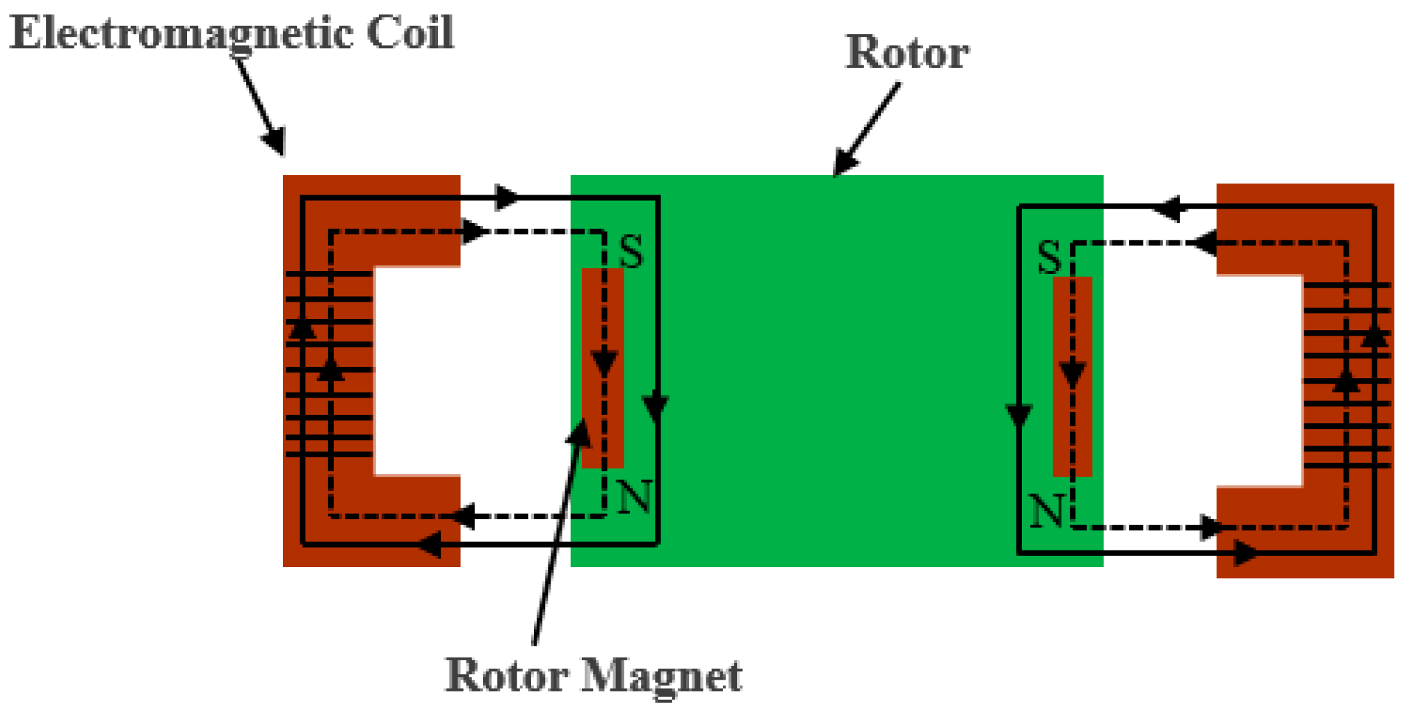
In Figure 2, the dashed and solid lines indicate the approximate distribution directions of magnetic fields for the permanent magnets and electromagnetic coils, respectively. The fundamental magnetic model is shown in Figure 3.
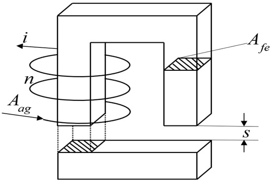
Figure 3.
Schematic diagram of the magnetic bearing system.
If the magnetic permeability within the magnetic circuit is constant, Ampère’s circuital law can be applied as follows:
The term in the equation is commonly referred to as the magnetomotive force (MMF), which serves as the “driving force” that compels magnetic flux through the magnetic circuit. In the following discussion, this is denoted as , and referred to as the MMF.
Since the magnetic flux density in the core and the air gap is identical, the magnetic field intensities and in Equation (1) can be expressed using the fundamental relationship between magnetic field intensity and magnetic flux density:
Solving the above equation yields the following:
Given that the relative permeability ur ≫ 1 in the core, the magnetization effect of the core is often negligible. Accordingly, the equation can be further simplified as follows:
2.2.2. Magnetic Force
When the magnetization of the core is neglected, the magnetic force under consideration differs from the Lorentz force acting on a conductor within a magnetic field. Instead, the interaction between magnets arises at the boundaries between media of differing magnetic permeabilities. The calculation of this type of force primarily relies on field energy theory.
The energy stored in the air gap volume , assuming a uniform magnetic field within the gap, is given by the following:
According to field energy theory, the force acting on a ferromagnetic material (where ur ≫ 1) results from the variation in field energy between the air gaps. This force is a function of the displacement of the magnetic element. For a small displacement , the magnetic flux remains constant.
However, when the air gap increases by , the volume increases, and the corresponding change in field energy must be supplied externally to overcome the attractive magnetic force. This force can therefore be expressed as the partial derivative of the magnetic energy with respect to the air gap , in accordance with the principle of virtual displacement:
In the simplest case where core magnetization is neglected, and with substituted from Equations (3) and (14), the resultant magnetic force becomes the following:
where .
This equation shows that the magnetic force is proportional to the square of both the current and the inverse of the square of the air gap. However, in some practical radial bearing coil configurations, there exists an angular deviation Δ between the two magnetic poles. Considering this angular effect, the final expression is modified as follows:
2.2.3. Transfer Model of a Single-Degree-of-Freedom System
To simplify the control model, independent control is applied to the two radial degrees of freedom, X and Y. The following derivation focuses on the system transfer function for one degree of freedom. Taking the X-axis as an example, based on Newton’s second law, the force balance equation for the magnetic bearing in the blood pump along a single degree of freedom can be written as follows:
where is the electromagnetic force along the X-axis, and is the external load force. For the purpose of this derivation, the load force is temporarily neglected. Substituting the electromagnetic force expression derived earlier in Equation (8), we obtain the following:
Through mathematical transformation, the transfer function of the system under current control can be derived as follows:
Since the above transfer function has an open-loop pole located in the right half of the -plane, according to the Routh stability criterion, feedback regulation must be introduced into the control system to ensure overall system stability.
2.3. Simulation Analysis of a Single-Degree-of-Freedom Magnetic Suspension System
Based on the theoretical derivation and calculation above, the current stiffness coefficient of the magnetic bearing system is , and the displacement stiffness coefficient is . An eddy current sensor is used for position detection, with an input range of 0.40 mm to 1.40 mm and an output current range of 4–20 mA. After current-to-voltage conversion, the output voltage range is 0.4–2 V. Therefore, the gain of the eddy current sensor is , and the delay time is . The transfer function of the eddy current sensor is expressed as follows:
Accordingly, the transfer function of the single-degree-of-freedom electromagnetic bearing system is as follows:
The transfer function of the power amplifier is as follows:
PID control has been widely applied in industry, and its control theory has been well developed. The structure of a PID controller is simple, consisting of three relatively independent parameters, and it does not require an exact mathematical model of the controlled system. The proportional component generates a control signal proportional to the error, the integral component eliminates steady-state error, and the derivative component enhances system responsiveness. The transfer function of the PID controller is given by the following:
where KP is the proportional gain, K1 the integral gain, and Kd the derivative gain.
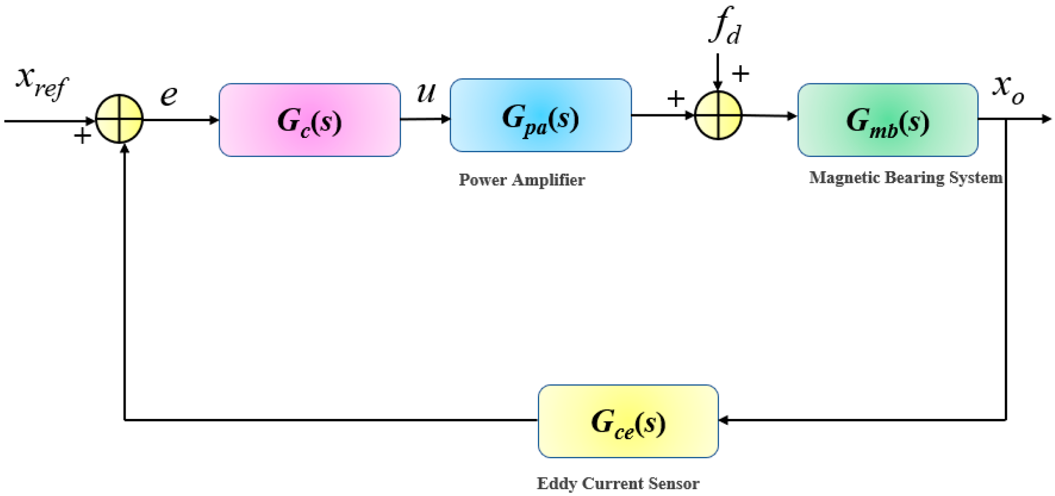
The closed-loop control system for the magnetic bearing is shown in Figure 4 below.

Figure 4.
Block diagram of the magnetic bearing closed-loop control system.
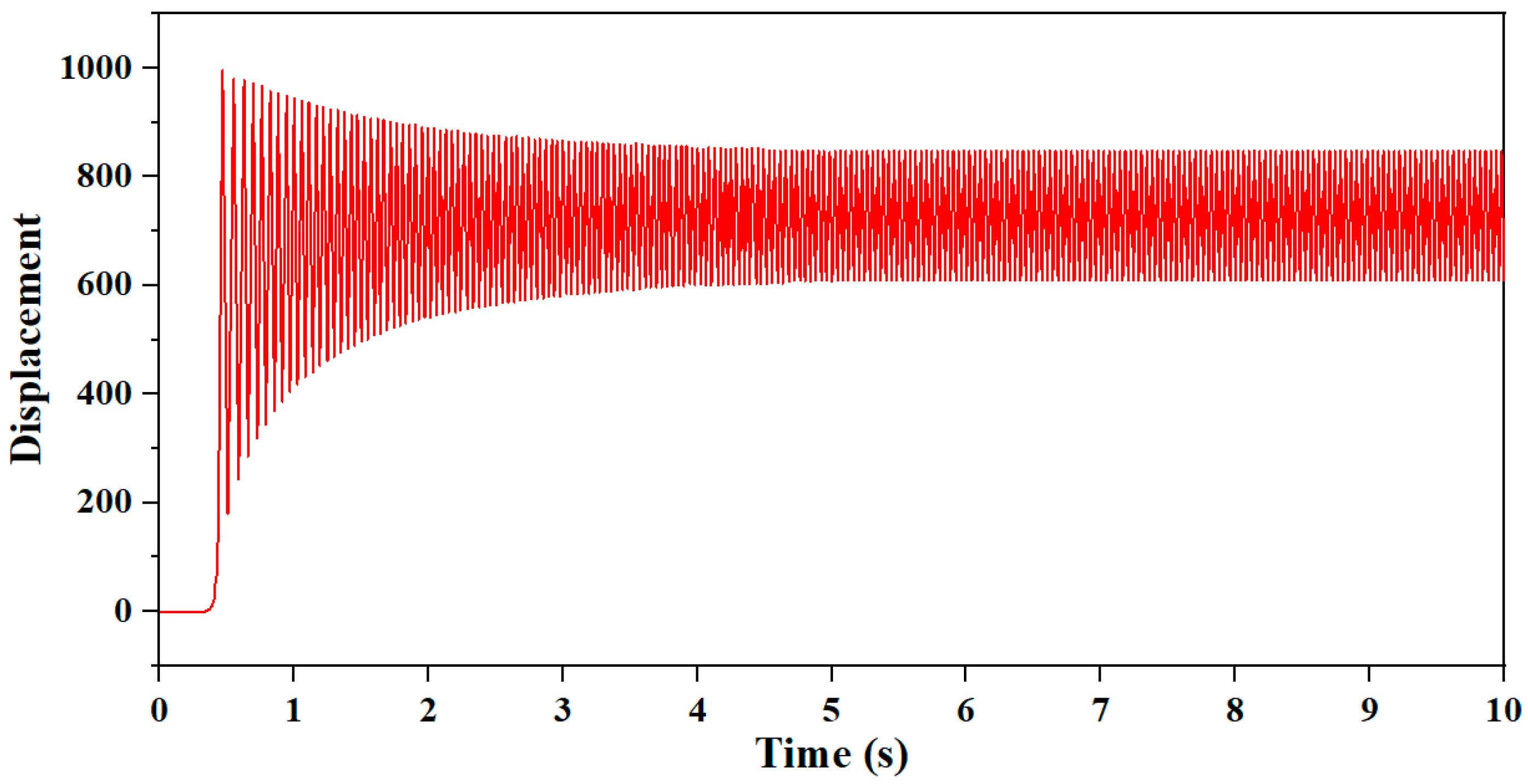
The simulation results of the single-degree-of-freedom system based on the block diagram above are shown in Figure 5.
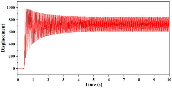
Figure 5.
Simulation results of the single-degree-of-freedom magnetic bearing system.
Although the simulation includes sensor-based feedback, the sensor itself acts as a low-pass system, which helps suppress high-frequency components and thus reduces high-frequency oscillation. However, due to the high gain of the sensor, low-frequency components are also amplified, resulting in underdamped system behavior. Therefore, it is necessary to further optimize the controller to adjust the system damping and improve the response characteristics.
3. Passive Stiffness Analysis and Model Parameter Correction Based on Finite Element Method
An analytical model for the electromagnetic force of the magnetic bearing was established based on magnetic circuit analysis and the principle of virtual work. By linearizing the magnetic field characteristics at the operating point, a differential-mode force expression was derived, leading to closed-form solutions for both force–displacement and force–current coefficients.
This theoretical model neglects radial X-Y magnetic field coupling, magnetic flux leakage, and saturation effects. Therefore, to verify the blood pump model, finite element simulations considering multiphysics coupling were conducted. In addition, to address the static support stiffness of hybrid magnetic bearings—which is difficult to analyze using classical passive theory—simulation results were used to further revise the theoretical model.
The following Table 1 presents the materials used in the electromagnetic simulations for this paper.

Table 1.
Material parameters for finite element simulation.
3.1. Magnetic Field Distribution in the Hybrid Magnetic Bearing
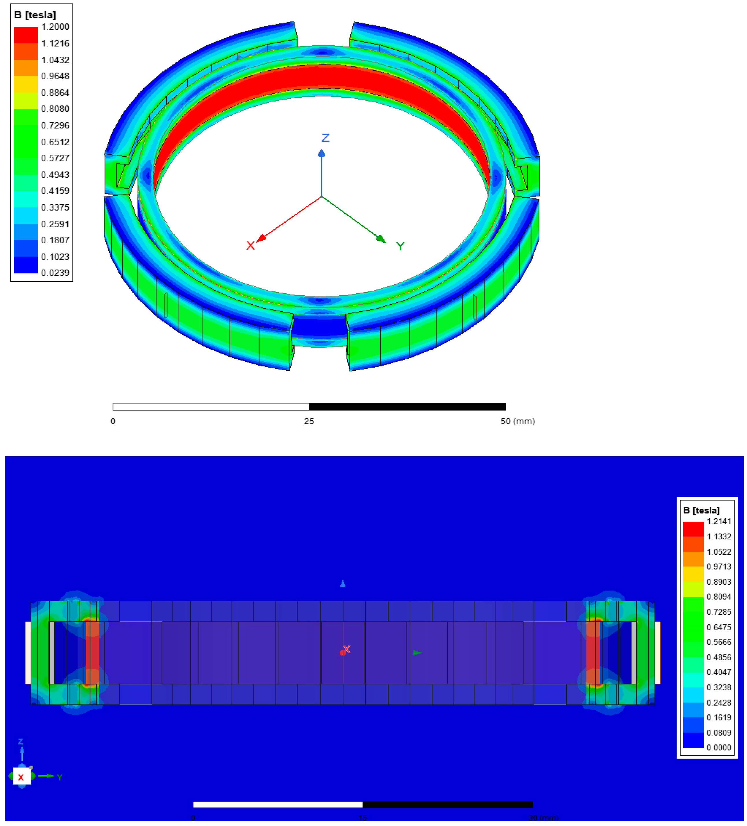
From the magnetic field contour plot in Figure 6, It can be observed that the magnetic field generated by the permanent magnets is mainly distributed along the loop formed by the permanent magnet, upper and lower iron rings, and the DT4 (high-purity soft iron) stator. The magnetic flux density at the top and bottom corners of the stator is nearly zero, indicating minimal field strength in those regions.
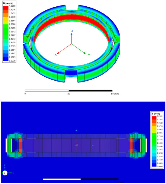
Figure 6.
Magnetic flux density contour of permanent magnet bias field (overall and XZ plane views).
This weakening at the edges is a typical manifestation of edge effects, where magnetic fields tend to diffuse inward or outward near the boundaries, leading to reduced field strength at the corners. Additionally, weak local magnetic loops are observed around the permanent magnets. These are caused by the air gaps between the stator and rotor, which facilitate partial flux leakage.
To analyze the magnetic field distribution, a circular path with a radius of 25.3 mm was defined around the permanent magnet as the integration path for field strength evaluation.
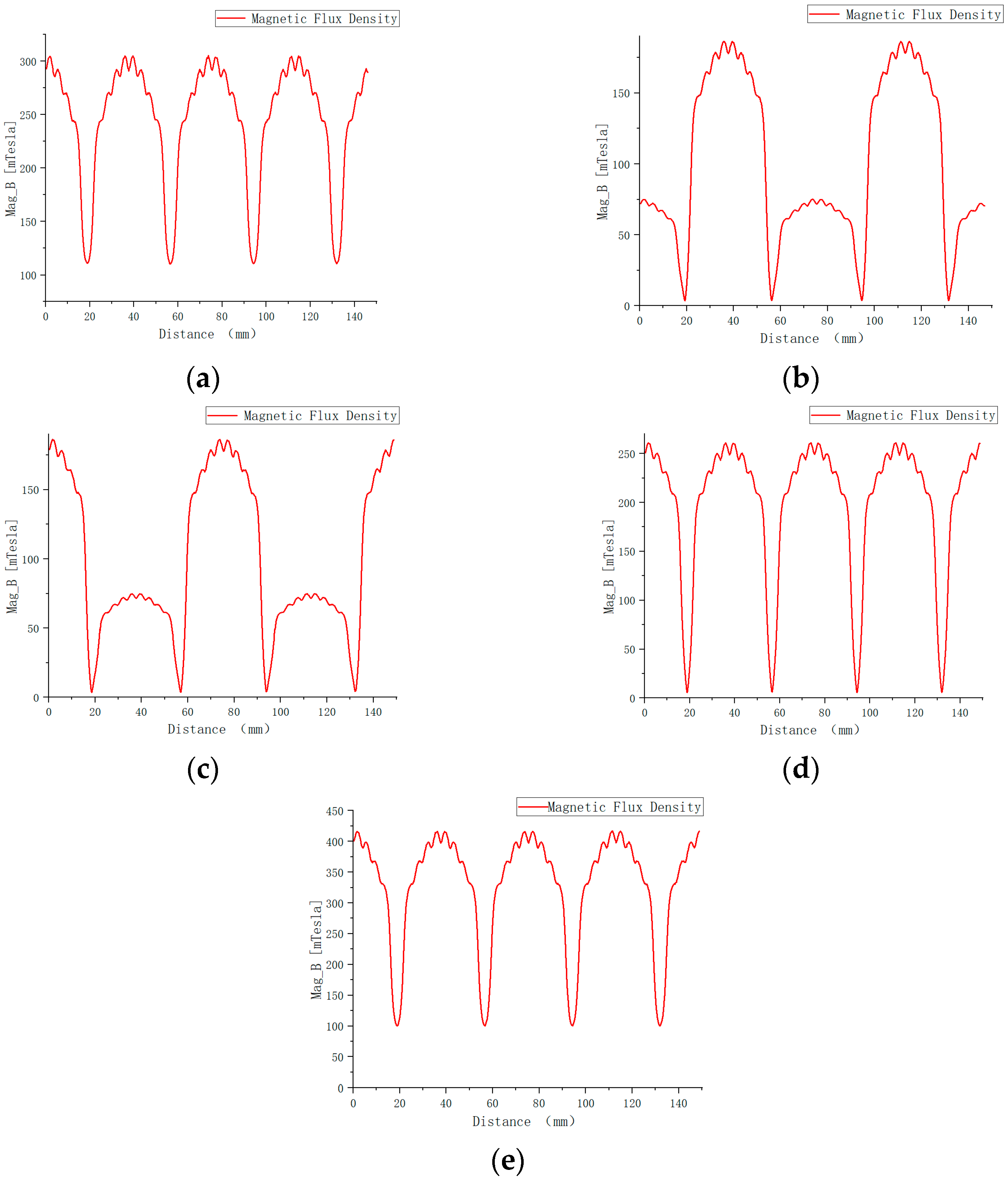
The results in Figure 7 show that the magnetic flux density distribution of the hybrid magnetic bearing is essentially the superposition of the fields from the permanent magnet and the electromagnetic coils. The overall pattern is symmetrical. Compared to the field generated by the permanent magnet or the coil alone, the resulting magnetic field strength is higher but not a simple linear sum.
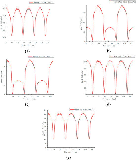
Figure 7.
Distribution curves of magnetic flux density along the path around the permanent magnet. (a) Permanent magnet; (b) 2 A bias current in X-direction; (c) 2 A bias current in Y-direction; (d) 2 A bias current in X- and Y-direction; (e) hybrid magnetic bearing.
The earlier theoretical model was based on a single-degree-of-freedom pure electromagnetic bearing and did not consider the influence of the permanent magnet’s field. The current magnetic field distribution of the hybrid magnetic bearing reveals evident magnetic coupling between the components. A quantitative analysis of its effect on bearing characteristics is presented below.
3.2. Passive Axial Stiffness Analysis
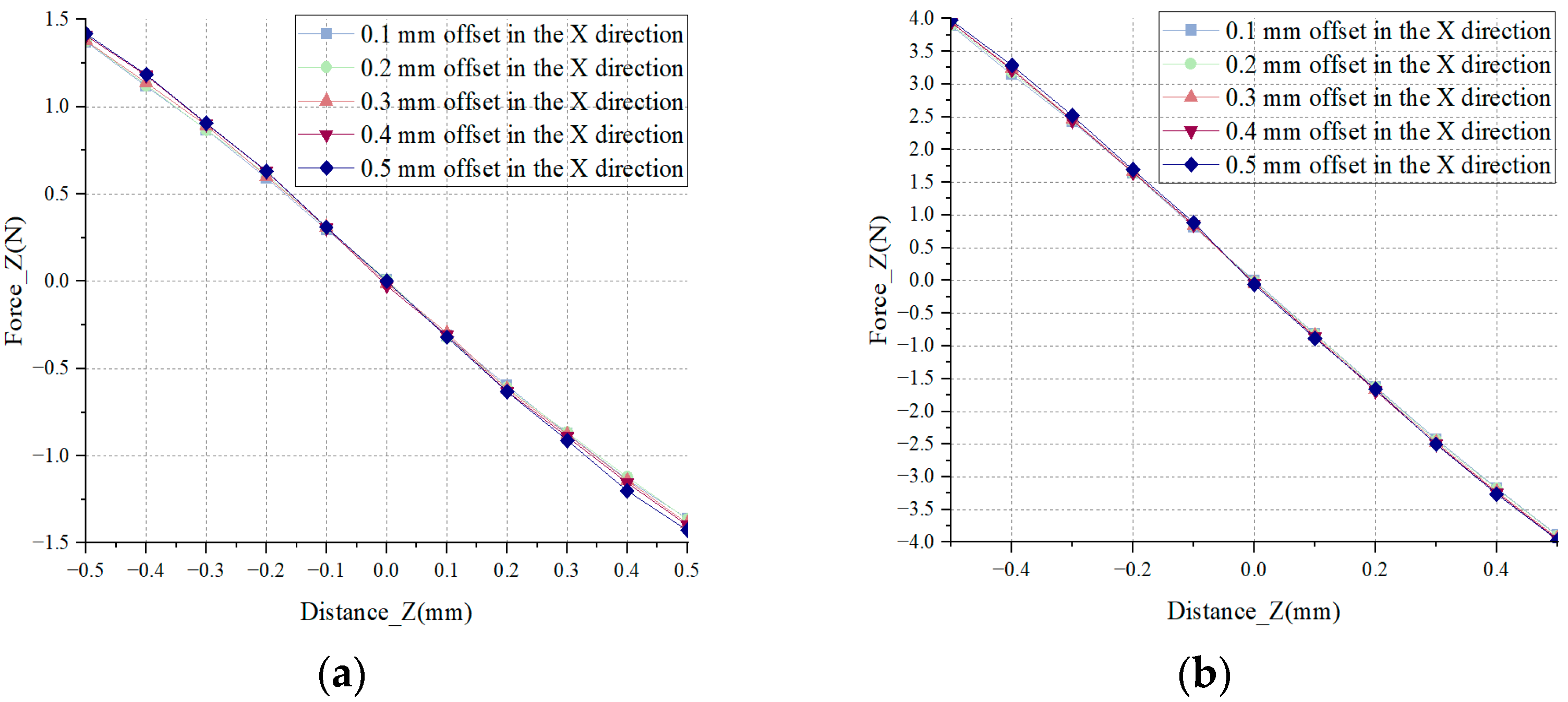
To investigate the static passive axial stiffness of the radial magnetic bearing, simulation analyses were conducted under two conditions, applying a 2 A bias current in a single direction and in both directions, while observing the influence of different radial positions on the axial force. Due to the symmetrical distribution of the magnetic field, only variations in the X-direction displacement were analyzed for their effect on axial stiffness. The simulation results are shown below (Figure 8).
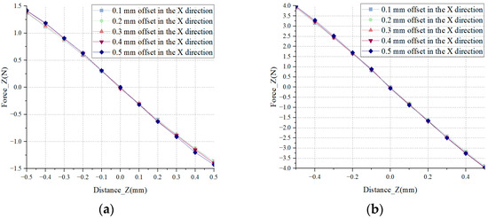
Figure 8.
Axial force vs. displacement curves under different radial offsets. (a) No bias current applied in X/Y coil; (b) 2 A bias current applied in both X and Y coils.
From the plots above, it can be observed that the axial force (Fz) and axial displacement (Dz) exhibit a linear negative correlation under the same radial offset. This indicates that a downward displacement of the rotor generates an upward restoring force, confirming that the magnetic bearing structure possesses passive axial support characteristics.
In the case without bias current in the X/Y directions, a radial offset of −0.5 mm results in an upward axial magnetic force of approximately 1.4 N, as shown in Figure 8. In contrast, when a 2 A bias current is applied in both X- and Y-directions, the same −0.5 mm radial offset produces an upward restoring force of approximately 4 N, as shown in Figure 8b.
Furthermore, the magnitude of the axial restoring force is largely unaffected by different radial offsets; it depends mainly on axial displacement. Across the full simulation range, the axial force maintains a nearly linear trend, regardless of radial offset. Therefore, within the linear region of 0–0.2 mm, a linear curve fitting was performed using the least-squares method to determine the axial support stiffness of the blood pump’s magnetic bearing:
3.3. Coupling Analysis of Force–Displacement and Force–Current Coefficients in the Radial Directions of the Blood Pump Magnetic Bearing
In the previous section, the radial magnetic field distribution along the X- and Y-directions was analyzed using magnetic flux density contours and field intensity plots. The results showed a symmetric magnetic field distribution, and that the electromagnetic coils in the X- and Y-directions do indeed exhibit magnetic coupling. Additionally, magnetic flux leakage and saturation effects were observed in the magnetic circuit.
This section further investigates how the magnetic field coupling in the Y-direction influences the stiffness (force–displacement coefficient) and force–current coefficient of the single-degree-of-freedom magnetic bearing system along the X-axis. Due to the symmetric nature of the magnetic field, the analysis is limited to how variations in current and displacement in the Y-direction affect system characteristics in the X-direction. The specific curve characteristics are shown in Figure 9 and Figure 10 respectively.
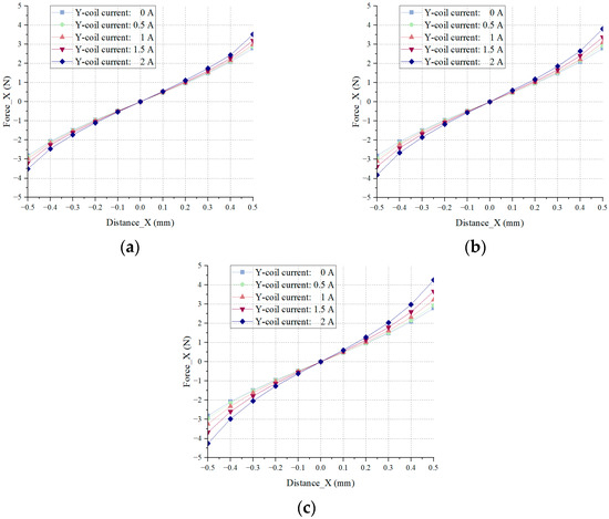
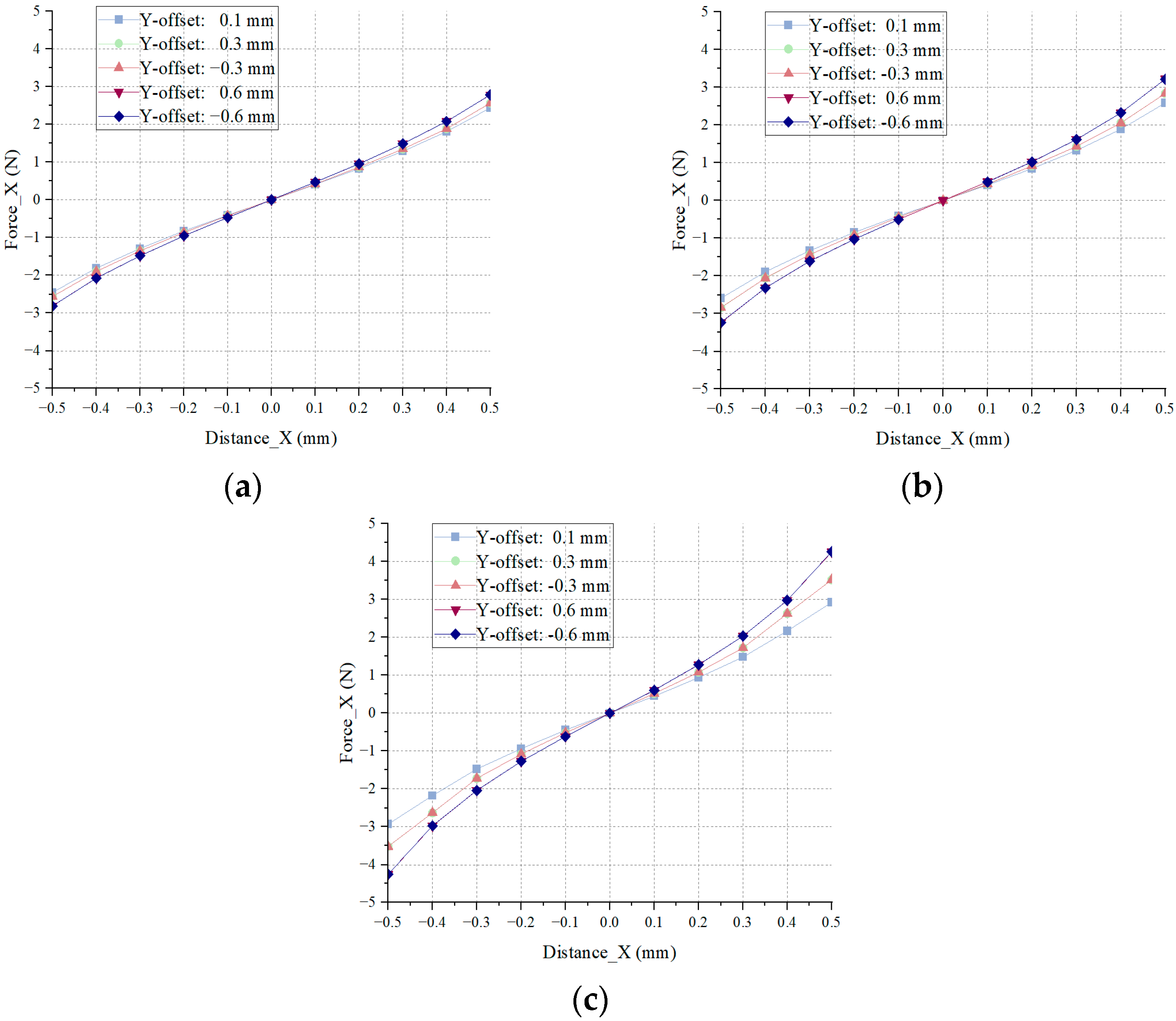
Figure 9.
Force–displacement curves in the X-direction under different Y-axis displacements: (a) Y-axis displacement = 0 mm; (b) Y-axis displacement = 0.3 mm; (c) Y-axis displacement = 0.6 mm.
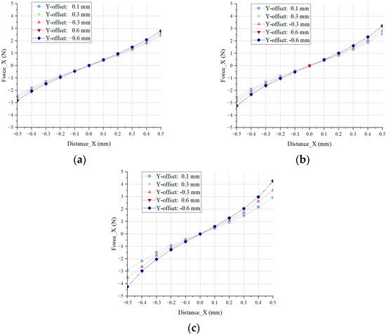
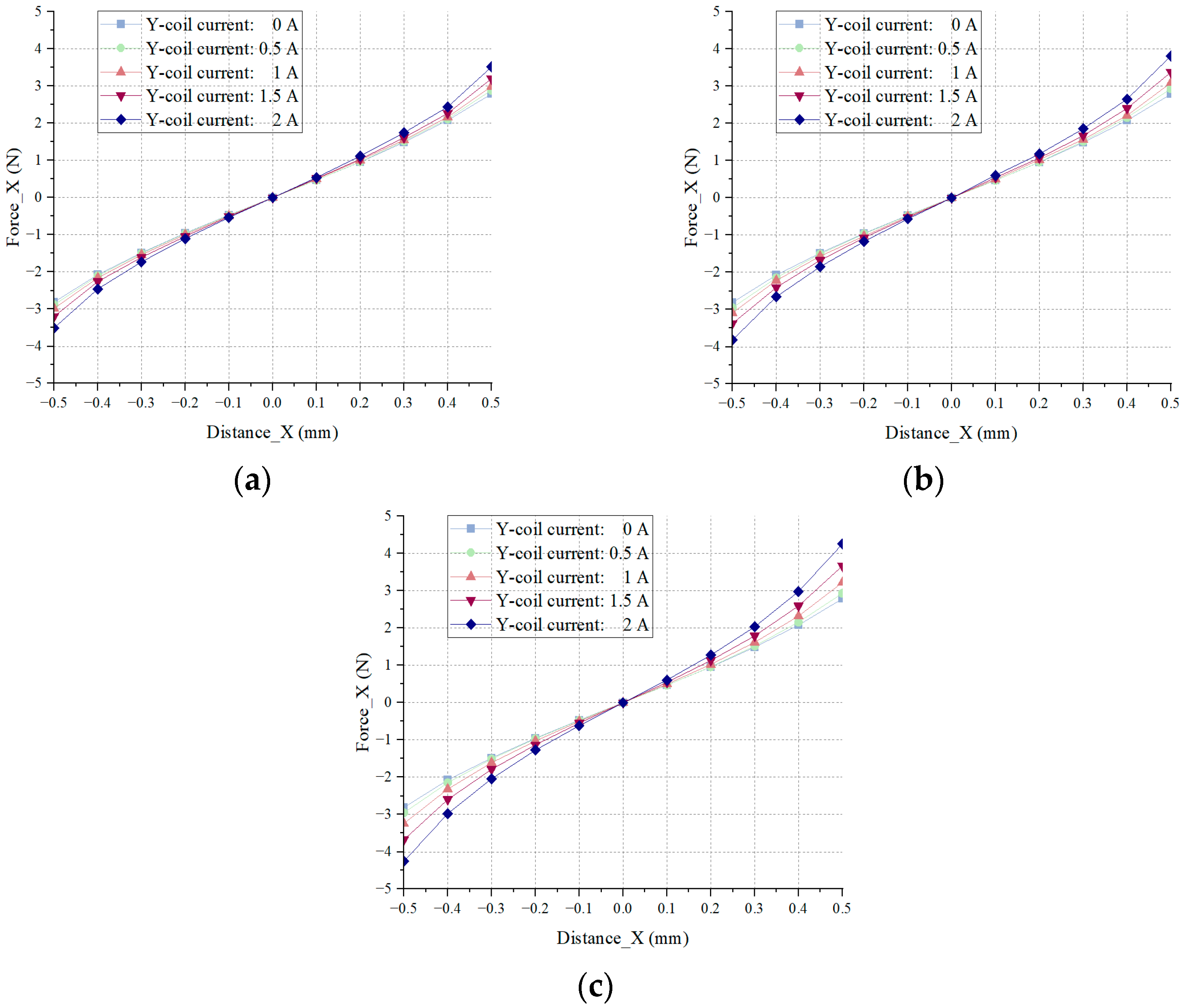
Figure 10.
Force–displacement curves in the X-direction under different Y-axis coil currents: (a) Y-axis current = 0 A; (b) Y-axis current = 1 A; (c) Y-axis current = 2 A.
When the Y-direction offset exceeds 0.3 mm, the system begins to show signs of reduced saturation. Therefore, the slope of the force–displacement curve in the linear region between 0.1 mm and 0.3 mm is fitted to characterize the effective force–displacement coefficient.
From Table 2 it can be observed that, at fixed Y-direction offset and current values, the slope of the force–displacement curve in the 0.1–0.3 mm range gradually increases. This indicates that, as the X-direction displacement increases, the axial force approaches a saturation point, where the system becomes magnetically saturated.
Table 2.
X-direction force (N) at different Y-direction offsets and coil currents.
While the Y-direction current or offset alone has a limited influence on the force–displacement coefficient, when both factors act simultaneously, the effect becomes significantly more pronounced.
It is evident in Table 3 that, when the Y-direction offset exceeds 0.3 mm and the current exceeds 1 A, the coupling effect significantly influences the force–displacement curve. Below this threshold, the maximum deviation remains under 13.33%, and the deviation decreases as the X-direction displacement decreases, with the minimum deviation occurring at 0.1 mm.
Table 3.
Deviation of force–displacement coefficient in the X-direction under various Y-direction conditions (relative to baseline: Y offset = 0, Y current = 0).
Based on the above analysis, it can be concluded that, within a certain linear range, the influence of the Y-direction offset and current on the force–displacement and force–current coefficients is limited. Therefore, the coefficients in this study were extracted at the ideal equilibrium position using electromagnetic simulation data.
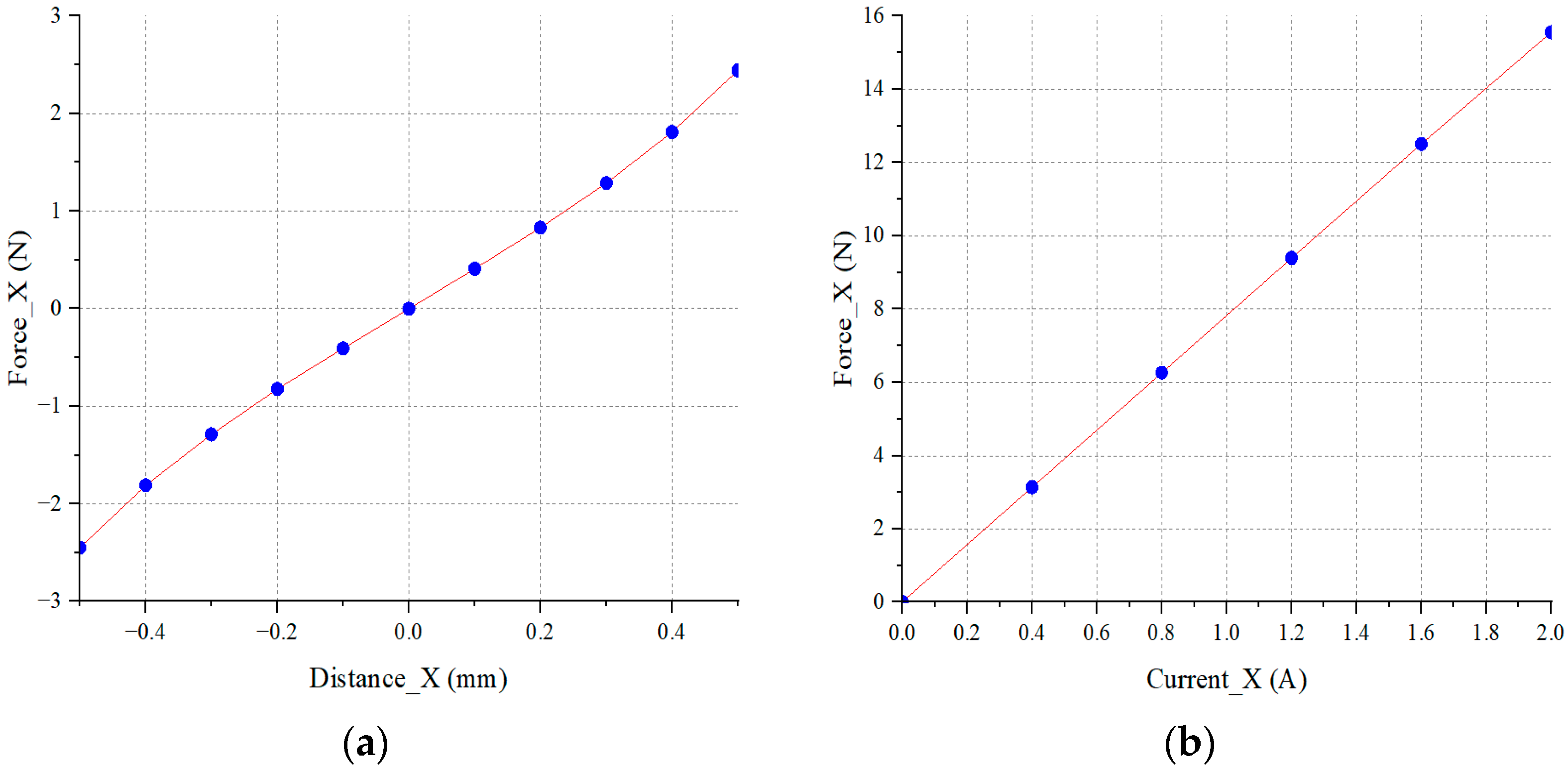
Based on the results of Figure 11, the derivative at the equilibrium point yields the stiffness coefficient as follows:
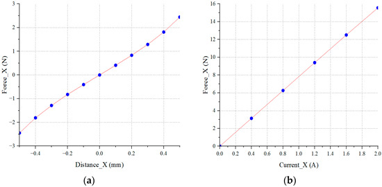
Figure 11.
Characteristic curves of the permanent magnet-biased magnetic bearing: (a) X-direction force–displacement curve at zero current; (b) X-direction force–current curve at equilibrium position.
Comparison with theoretical values shows that the FEM-corrected coefficients are slightly lower. This deviation is primarily attributed to magnetic flux leakage.
4. Two Optimization Methods for PID Controller
Previous simulation results indicate that the single-degree-of-freedom magnetic bearing system is inherently open-loop unstable. To ensure stable system operation, a PID control strategy is introduced to achieve closed-loop regulation. The effectiveness of PID control relies on the coordinated optimization of the proportional, integral, and derivative components. A dynamic balance must be maintained among these components. However, conventional PID parameters often depend heavily on empirical tuning and tend to perform poorly in controlling nonlinear systems.
To address these issues, this study introduces two self-tuning methods based on backpropagation (BP) neural networks and the particle swarm optimization (PSO) algorithm to optimize PID parameters adaptively.
4.1. BP Neural Network-Based PID Controller
The strong nonlinear mapping capability of BP neural networks enables the learning of system dynamics to determine an optimal combination of PID parameters. The basic working principle is as follows:
Input data pass through the network and are processed layer by layer to generate an output. This output is then compared to the actual target value to compute an error. The error is propagated backward through the network, and the gradient descent method is used to iteratively adjust the weights and biases of each neuron layer by layer. This process continues until the network output gradually converges to the desired value.
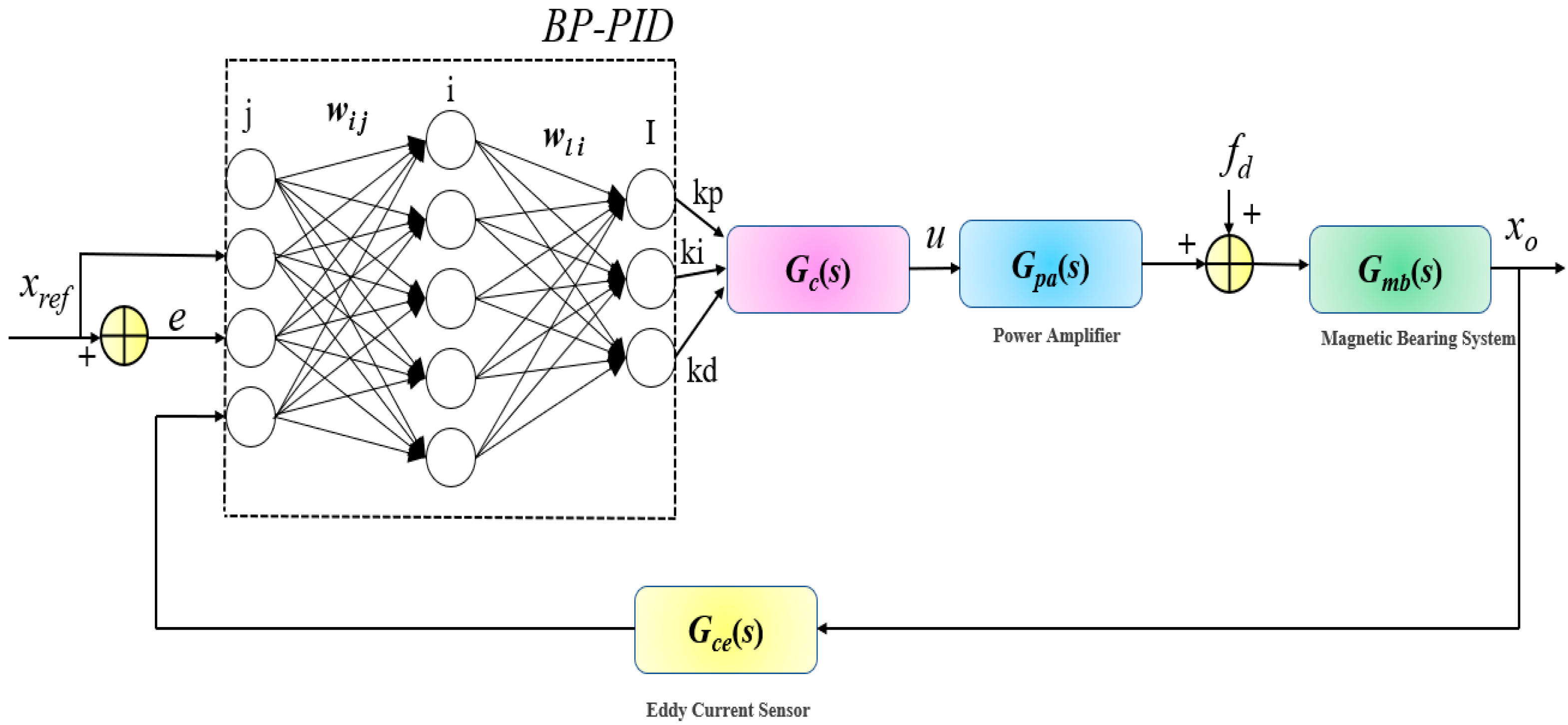
The core of this method lies in computing the gradient of the error with respect to the network parameters via the chain rule, which enables effective parameter optimization and adaptive learning of the controller. The framework is described in Figure 12 below:
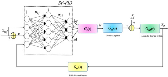
Figure 12.
Structure of the BP neural network.
Input layer (four neurons):
Hidden layer weights:
where is a randomly initialized 5×4 matrix.
Output layer weights:
Hidden layer outputs:
Hidden layer outputs:
Output layer outputs:
where
Activation function for the hidden layer:
Activation function for the output layer:
- Role of activation functions:
The activation function transforms the weighted sum of the input signals into the neuron’s output (analogous to neurotransmitter release or signal normalization).
The loss function serves as a performance metric to evaluate the learning effectiveness of the neural network.
Here, 0.5 is a scaling factor for the error, which can affect the convergence speed and stability of the optimization algorithm.
A smaller loss value helps ensure stable training by avoiding excessively large gradient updates, which could otherwise cause instability or oscillations.
According to the gradient descent method, the weight coefficients are updated by searching along the negative gradient of the error function E(k) with respect to the weights. Additionally, a momentum term is introduced to accelerate convergence, resulting in the following learning rule for the output layer weights:
where
n: learning rate;
a: momentum coefficient.
- Chain rule (backpropagation):
Since is unknown, it is approximated using the sign function ). The inaccuracy introduced by this approximation can be compensated by adjusting the learning rate n.
Given
then
Here, denotes the derivative of the activation function at the output layer, and is the specific form used in this case.
4.2. PSO-Based PID Neural Network Controller
To evaluate the performance of the BP-PID controller and address the limitation of conventional PID tuning methods prone to local optima, this study also designs a global PID parameter optimization strategy based on the particle swarm optimization (PSO) algorithm. This approach leverages the global search capability of PSO and employs swarm intelligence to automatically tune the PID controller parameters, effectively avoiding the risk of local minima commonly encountered in traditional optimization techniques.
4.2.1. Principle of the Particle Swarm Optimization Algorithm
The particle swarm optimization (PSO) algorithm is a population-based optimization technique inspired by the foraging behavior of bird flocks. In PSO, each particle represents a candidate solution and possesses two properties: position and velocity. The position corresponds to a potential solution, while the velocity determines the particle’s movement direction and step size in the next iteration.
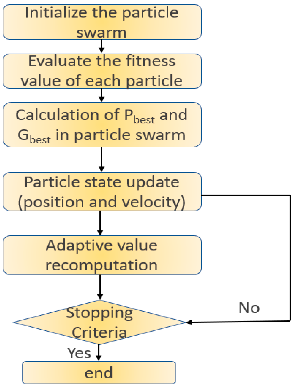
The optimization process begins by initializing the positions and velocities of all particles in the swarm. Then, during each iteration, the fitness of every particle is calculated based on a defined performance metric. Particles update their velocities and positions based on their own best-known position and the global best-known position. This process repeats until a stopping criterion is met. The position of the globally best-performing particle is selected as the optimal solution. The detailed procedure is illustrated in Figure 13.
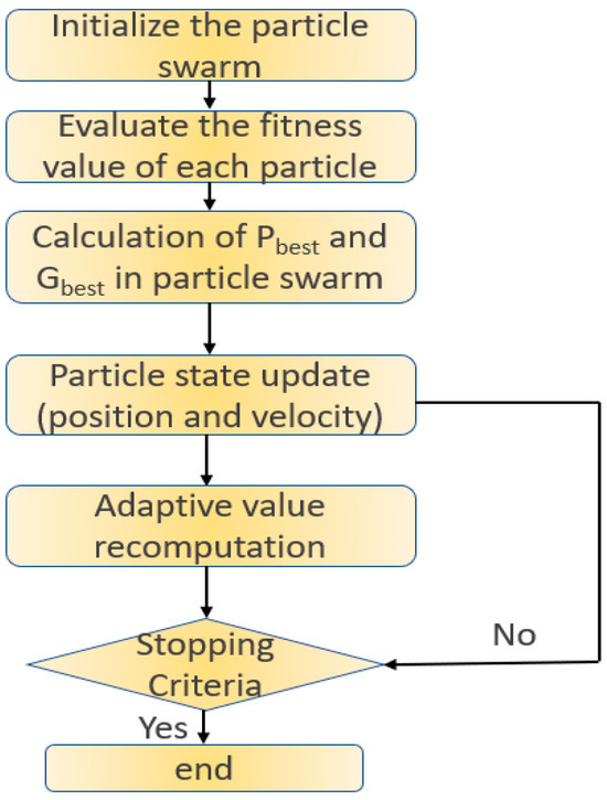
Figure 13.
Flowchart of PID parameter optimization using PSO algorithm.
4.2.2. Steps for Computing Optimal PID Parameters Using PSO
- Initialize the particle swarm:
Set the population size, initial positions, and velocities of the particles. The initialization equations are as follows:
Here, ub and lb are the upper and lower bounds of particle positions, and Vmin and Vmax are the minimum and maximum velocity bounds.
- Evaluate fitness:
For each particle (representing a set of PID parameters), compute the controller’s performance metrics such as the sum of squared errors (SSE) or settling time. These serve as the particle’s fitness value.
- Update particle velocity and position:
Based on PSO update equations,
where w is the inertia weight, and C1 and C2 are cognitive and social learning factors.
- Position update:
- Check termination criteria:
If the maximum number of iterations is reached or the fitness meets the desired threshold, the process terminates. Otherwise, repeat the update process.
- Output the optimal solution:
The position of the globally best particle is selected as the optimal PID parameter set (Kp, Ki, Kd).
5. Simulation and Experiments
- Simulation Analysis of the Magnetic Bearing Control System
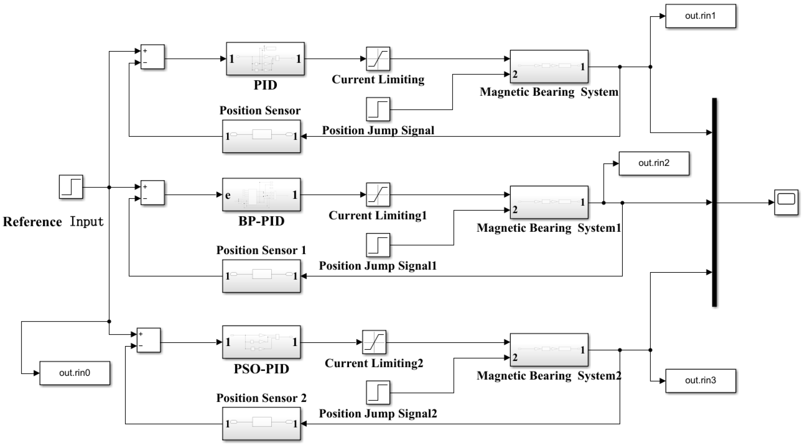
After simulating the single-degree-of-freedom magnetic bearing system, it was found that—even with sensor feedback—the system remained underdamped. As the system is a typical single-input single-output (SISO) system, a PID controller can be introduced for compensation. Furthermore, based on previous electromagnetic simulations, the model parameters were corrected to account for effects such as magnetic coupling and flux leakage. The two previously designed PID controllers were implemented in simulation (Figure 14).
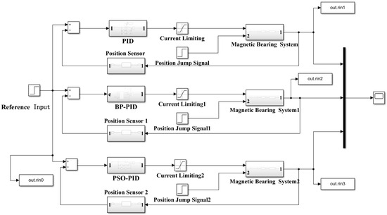
Figure 14.
Magnetic suspension control simulation diagram of the blood pump.
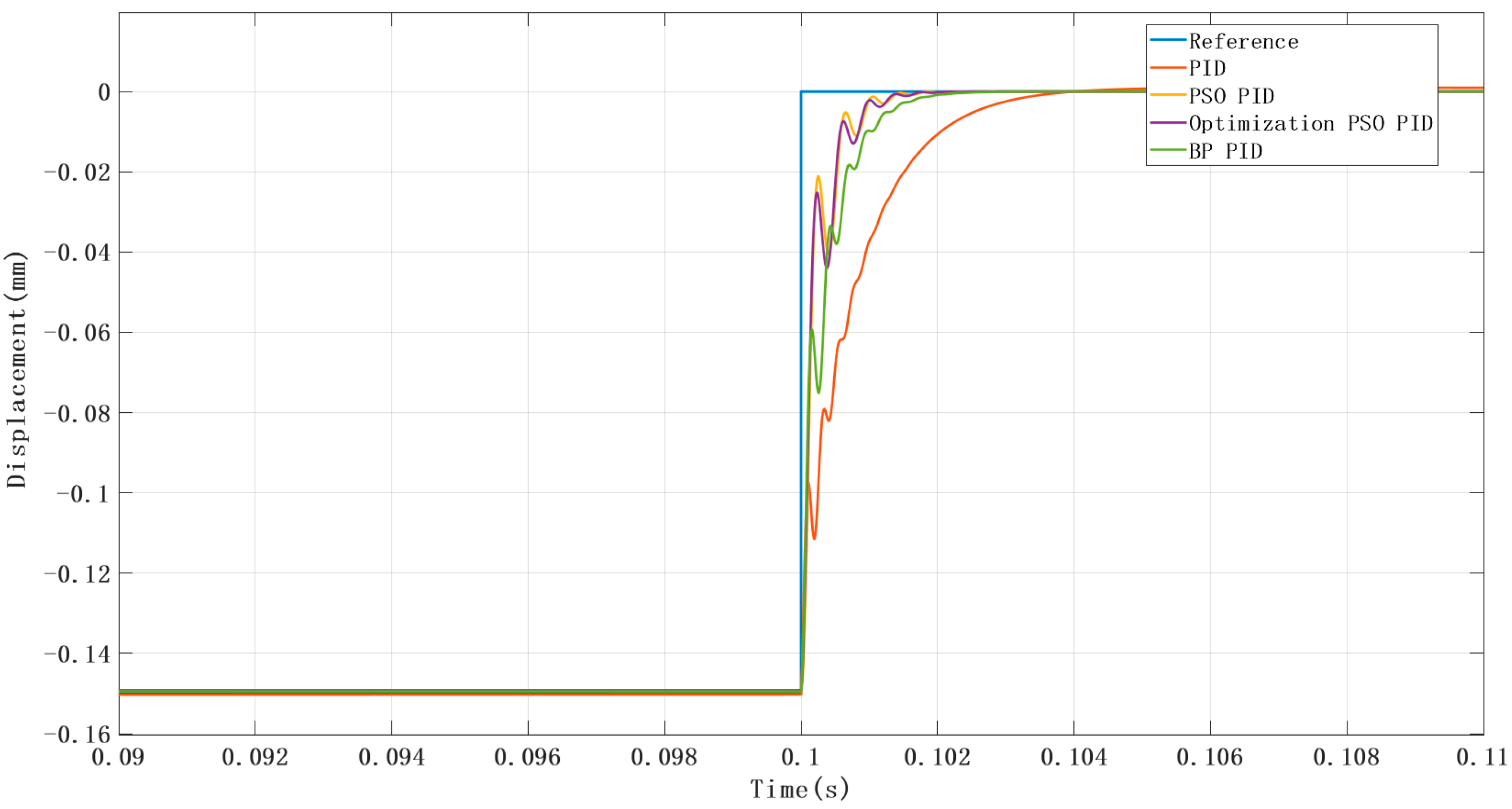
At t = 0.1 s, a reference displacement input was applied to the system, changing abruptly from −0.15 mm to 0 mm. The simulation result is shown below (Figure 15).
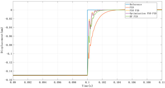
Figure 15.
Step response output of the system.
System performance metrics are listed in Table 4.To achieve a more stable system response, the system was tuned toward an overdamped state. Except for the manually tuned PID controller, the other three optimization methods resulted in negligible overshoot. As shown in the performance metrics above, all three optimized PID controllers outperformed the manually tuned PID in terms of control performance.
Table 4.
System performance metrics.
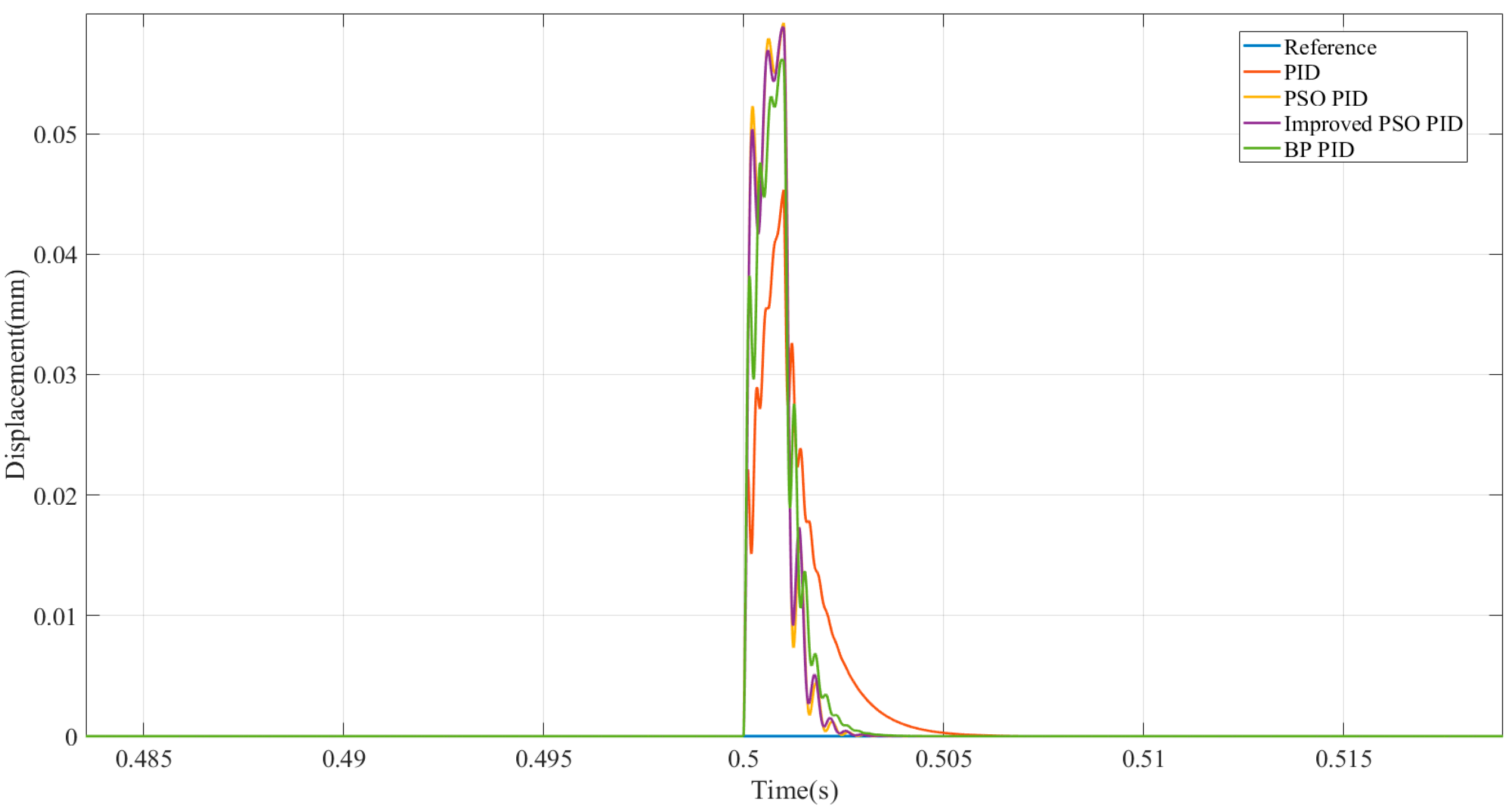
The Figure 16 below shows the output response curve when an impulse excitation is applied at 0.5 s during the simulation.
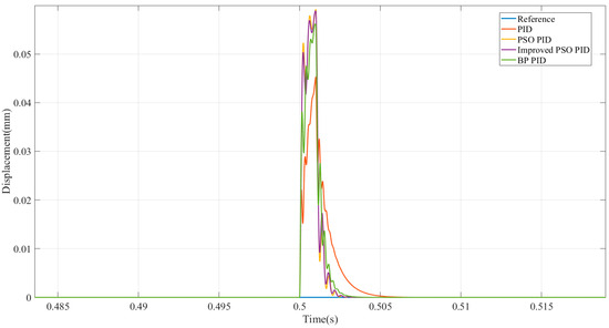
Figure 16.
Impulse response output of the system.
Among them, the improved PSO-PID achieved the best rise time and settling time, while the BP-PID exhibited superior performance in suppressing system oscillations.
Figure 16 simulates the system impulse response output, demonstrating that the optimized control strategy adopted in this study achieves rapid compensation for sudden disturbances compared to conventional PID control.
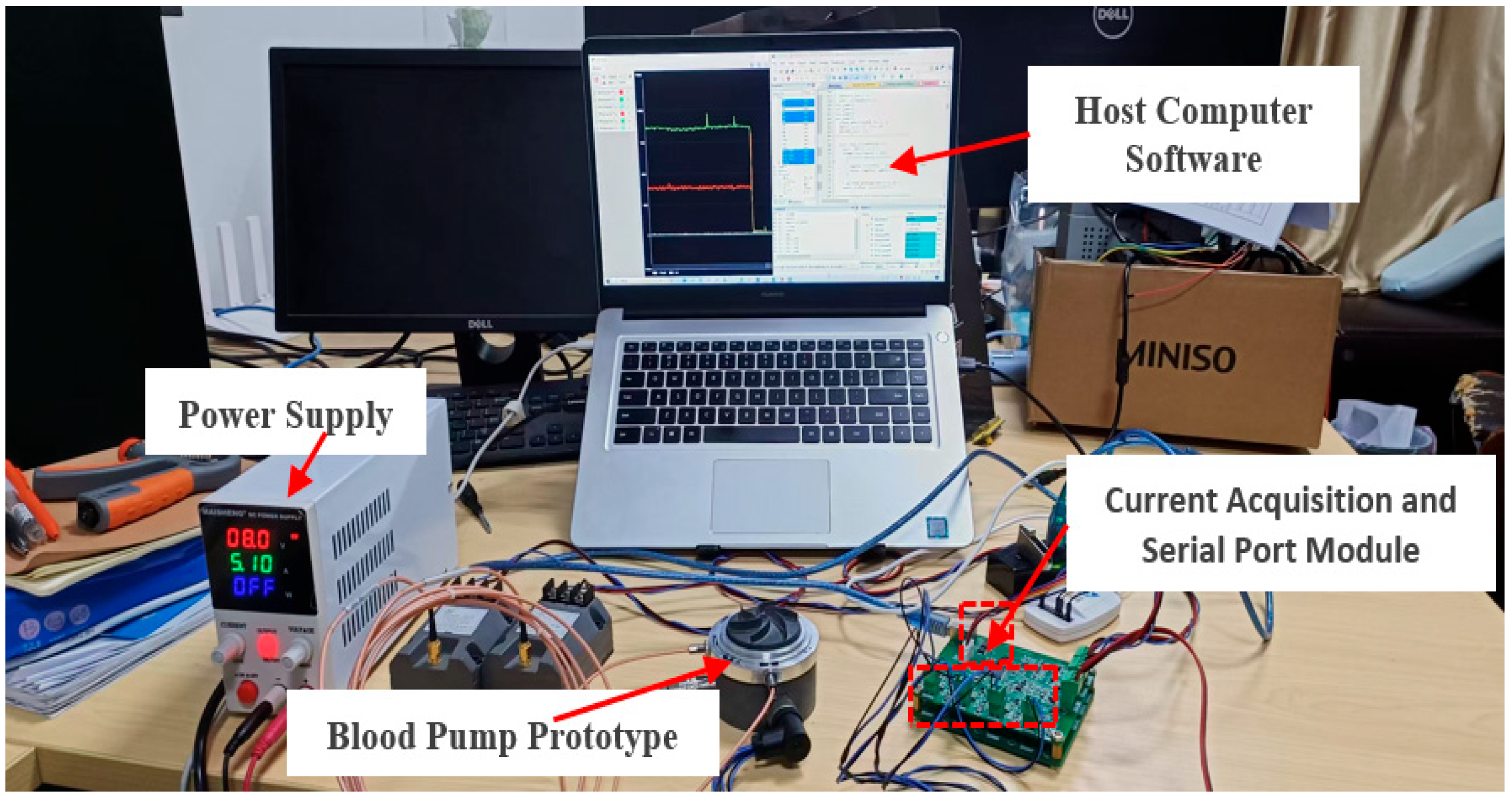
The hardware configuration of the magnetically levitated blood pump test bench primarily consists of the following components, as shown in the Figure 17 below: the blood pump, Position Sensor, Current Sensor, DRV884H H-Bridge Driver (for driving coil current), STM32 Master Control System (core controller), 5–24 V Adjustable Power Module, and PC.

Figure 17.
Hardware of control system for magnetically levitated blood pump.
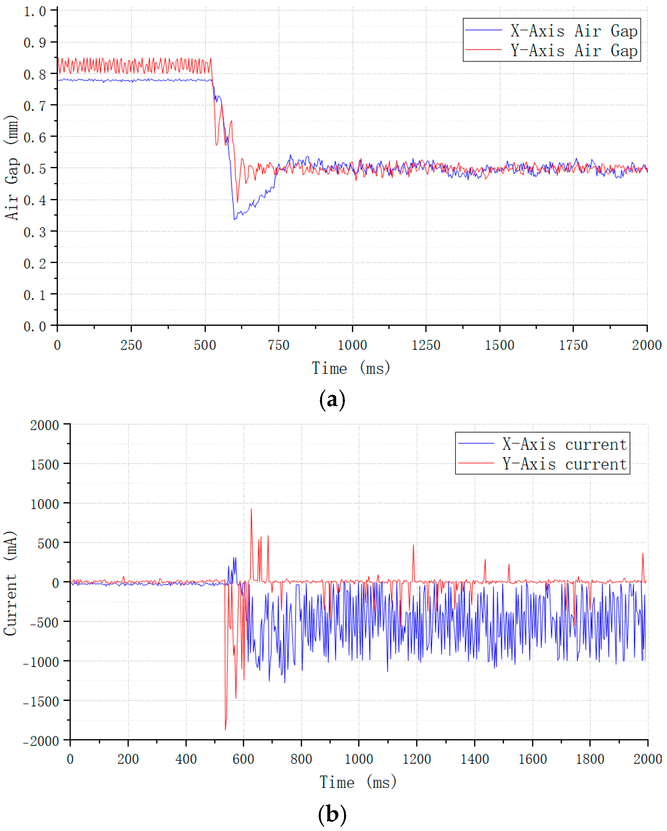
Based on this established hardware platform, we conducted magnetic levitation experiments on the blood pump, the results of which are presented in the Figure 18 below.
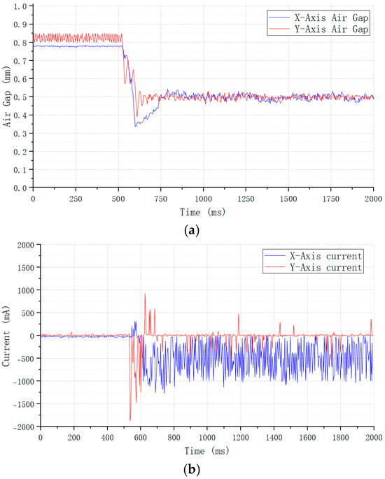
Figure 18.
Experimental results of the levitation process in a two-degree-of-freedom magnetic levitation system: (a) X-direction force–displacement curve at zero current; (b) X-direction force–current curve at equilibrium position.
Figure 18 presents the variation in current and air gap observed during a two-degree-of-freedom magnetic levitation experiment. The results demonstrate rapid rotor levitation, achieving stabilization with a transition time of about 70 ms. A discrepancy exists between the experimental and simulation results, attributable primarily to practical factors including machining tolerances and installation errors. Nevertheless, the overall dynamic trends remain consistent. Throughout the levitation process, the electromagnet coil current exhibits significant dynamics, undergoing an initial surge during the startup phase to establish positioning, followed by fine-tuning within a narrow operating range to maintain precise rotor position control at equilibrium. This behavior indicates that the self-tuned PID parameters yield superior dynamic response coupled with high steady-state accuracy.
6. Conclusions and Discussion
A finite element simulation analysis showed that, near the rotor’s equilibrium position (air gap < 0.3 mm, control current < 2 A), the influence of radial magnetic coupling is relatively small (relative error ≤ 10%), which validates the rationality of the linearized modeling approach. Closed-loop system simulations using corrected model parameters indicated that the system exhibits typical underdamped behavior. The introduction of intelligent optimization algorithms effectively reduced the subjectivity and uncertainty associated with manual PID tuning, enhancing controller reliability and robustness.
The simulation results demonstrate that the PID controller optimized via the improved particle swarm optimization (PSO) algorithm offers significant advantages in the control of magnetically levitated blood pump systems. Compared with BP neural network optimization and conventional manual tuning, the improved PSO-based controller achieves better performance in both dynamic response and steady-state accuracy. Specifically, it achieved a rise time of 0.0049 s, a settling time of 0.0079 s, and a steady-state error of 0.0013 mm.
The intelligent optimization control strategy proposed in this study has shown promising performance in simulation environments; however, its real-world applicability remains dependent on the accuracy of the underlying mathematical model. Key concerns include the following:
- Whether the model sufficiently captures the system’s dynamic behavior, including higher-order modes and unmodeled nonlinearities;
- Whether the parameter identification process accurately reflects the system’s physical characteristics;
- The potential impact of unmodeled dynamics—such as external disturbances or variations in material properties—on control stability.
Although the improved PSO algorithm demonstrated superior results in simulation, further experimental validation is required to confirm its transferability to actual blood pump systems. Additionally, under extreme operating conditions—such as large currents or wide air gaps—the effects of magnetic coupling and flux leakage may become more pronounced. Future work should incorporate multiphysics coupling analysis to provide a more comprehensive evaluation. To account for magnetic coupling effects and flux leakage across varying positions, a nonlinear magnetic force model should be developed to further optimize the controller. External vibrations, sensor noise, and temperature-induced parameter drift should be further accounted for in model refinement and controller design.
Air levitation experiments were further included in this study to provide initial validation of the proposed algorithm’s effectiveness. The current investigation, however, did not evaluate control stability under clinically relevant physiological disturbances—particularly acute hypertensive episodes or substantial alterations in peripheral vascular resistance. Establishing system robustness against such perturbations therefore represents a critical direction for future research.
Author Contributions
Conceptualization, T.J. and Y.Y.; methodology, T.J. and Y.Y.; software, Y.Y. and W.R.; validation, W.R. and Y.Y.; writing—original draft preparation, Y.Y.; writing—review and editing, T.J. and Y.Y.; visualization, Y.Y.; supervision, W.R. and T.J. All authors have read and agreed to the published version of the manuscript.
Funding
This research received no external funding.
Institutional Review Board Statement
Not applicable.
Informed Consent Statement
Not applicable.
Data Availability Statement
Data are contained within the article. The data presented in this study can be requested from the authors.
Acknowledgments
The authors want to thank the study participants for taking part in the study.
Conflicts of Interest
The authors declare no conflicts of interest.
References
- Masuzawa, T.; Ezoe, S.; Kato, T.; Okada, Y. Magnetically suspended centrifugal blood pump with an axially levitated motor. Artif. Organs 2003, 27, 631–638. [Google Scholar] [CrossRef] [PubMed]
- Masuzawa, T. Magnetically suspended motor system applied to artificial hearts and blood pumps. Proc. Inst. Mech. Eng. Part I J. Syst. Control Eng. 2016, 231, 330–338. [Google Scholar] [CrossRef]
- Levine, A.; Gass, A. Third-Generation LVADs: Has Anything Changed? Cardiol. Rev. 2019, 27, 293–301. [Google Scholar] [CrossRef] [PubMed]
- Kim, S.H.; Hashi, S.; Ishiyama, K. Actuation of Novel Blood Pump by Direct Application of Rotating Magnetic Field. IEEE Trans. Magn. 2012, 48, 1869–1874. [Google Scholar] [CrossRef]
- Zhao, X.; Deng, Z.; Wang, X.; Mei, L. Research status and development of permanent magnet biased magnetic bearings. Diangong Jishu Xuebao/Trans. China Electrotech. Soc. 2009, 24, 9–20. [Google Scholar]
- Zhi, C.; Huang, Y.; Guo, B.; Dong, J.; Peng, F. Performance Comparison of Analytical Models for Rotor Eccentricity: A Case Study of Active Magnetic Bearing. J. Magn. 2020, 25, 285–292. [Google Scholar]
- Wang, H.; Wu, Z.; Liu, K.; Wei, J.; Hu, H. Modeling and Control Strategies of a Novel Axial Hybrid Magnetic Bearing for Flywheel Energy Storage System. IEEE/ASME Trans. Mechatron. 2022, 27, 3819–3829. [Google Scholar] [CrossRef]
- Earnshaw, S. On the Nature of the Molecular Forces which Regulate the Constitution of the Luminiferous Ether. Tcaps 1848, 7, 97. [Google Scholar]
- Masuzawa, T.; Kita, T.; Matsuda, K.; Okada, Y. Magnetically suspended rotary blood pump with radial type combined motor-bearing. Artif. Organs 2000, 24, 468–474. [Google Scholar] [CrossRef] [PubMed]
- Duncan, B.W. Pediatric mechanical circulatory support: A new golden era? Artif. Organs 2005, 29, 925–926. [Google Scholar] [CrossRef] [PubMed]
- Hoshi, H.; Shinshi, T.; Takatani, S. Third-generation blood pumps with mechanical noncontact magnetic bearings. Artif. Organs 2006, 30, 324–338. [Google Scholar] [CrossRef] [PubMed]
- Han, J.; Li, Y.; Lin, Y.; Zhang, N.; Xiong, F. Research on tuning method of PID controller parameter for hybrid magnetic bearing. J. Mech. Sci. Technol. 2024, 38, 931–941. [Google Scholar] [CrossRef]
- Wu, Y.; Ren, G.-P.; Zhang, H.-T. Dual-mode predictive control of a rotor suspension system. Sci. China Inf. Sci. 2019, 63, 112204. [Google Scholar] [CrossRef]
- Ying-Xin, Y.; Guang-Ren, D. Robust control of magnetic bearing with gyroscopic effects using output feedback controller. In Proceedings of the 2006 1st International Symposium on Systems and Control in Aerospace and Astronautics, Harbin, China, 19–21 January 2006; pp. 5–782. [Google Scholar]
- Chen, M.; Knospe, C.R. Control Approaches to the Suppression of Machining Chatter Using Active Magnetic Bearings. IEEE Trans. Control Syst. Technol. 2007, 15, 220–232. [Google Scholar] [CrossRef]
- Donati, G.; Basso, M.; Mugnaini, M.; Neri, M.O. Automatic Tuning of Augmented PIDs for Active Magnetic Bearings Supporting Turbomachinery. IEEE/ASME Trans. Mechatron. 2025, 30, 1765–1775. [Google Scholar] [CrossRef]
- Miras, J.D.; Join, C.; Fliess, M.; Riachy, S.; Bonnet, S. Active magnetic bearing: A new step for model-free control. In Proceedings of the 52nd IEEE Conference on Decision and Control, Firenze, Italy, 10–13 December 2013; pp. 7449–7454. [Google Scholar]
- Basaran, S.; Sivrioglu, S. Novel repulsive magnetic bearing flywheel system with composite adaptive control. IET Electr. Power Appl. 2019, 13, 676–685. [Google Scholar] [CrossRef]
- Hutterer, M.; Wimmer, D.; Schrödl, M. Stabilization of a Magnetically Levitated Rotor in the Case of a Defective Radial Actuator. IEEE/ASME Trans. Mechatron. 2020, 25, 2599–2609. [Google Scholar] [CrossRef]
- Chen, L.; Zhu, C.; Zhong, Z.; Wang, C.; Li, Z. Radial position control for magnetically suspended high-speed flywheel energy storage system with inverse system method and extended 2-DOF PID controller. IET Electr. Power Appl. 2020, 14, 71–81. [Google Scholar] [CrossRef]
- Gupta, S.; Biswas, P.K.; Debnath, S.; Ghosh, A.; Babu, T.S.; Zawbaa, H.M.; Kamel, S. Metaheuristic Optimization Techniques Used in Controlling of an Active Magnetic Bearing System for High-Speed Machining Application. IEEE Access 2023, 11, 12100–12118. [Google Scholar] [CrossRef]
- Mao, Z.; Suzuki, S.; Nabae, H.; Miyagawa, S.; Suzumori, K.; Maeda, S. Machine learning-enhanced soft robotic system inspired by rectal functions to investigate fecal incontinence. Bio-Des. Manuf. 2025, 8, 482–494. [Google Scholar] [CrossRef]


Disclaimer/Publisher’s Note: The statements, opinions and data contained in all publications are solely those of the individual author(s) and contributor(s) and not of MDPI and/or the editor(s). MDPI and/or the editor(s) disclaim responsibility for any injury to people or property resulting from any ideas, methods, instructions or products referred to in the content. |
© 2025 by the authors. Licensee MDPI, Basel, Switzerland. This article is an open access article distributed under the terms and conditions of the Creative Commons Attribution (CC BY) license (https://creativecommons.org/licenses/by/4.0/).