1. Introduction
Rotating machinery is a critical component of mechanical systems and is widely used in industrial applications [
1,
2]. With the growing complexity and intelligence of mechanical systems, the unexpected failures of rotating machinery can lead to severe economic loss and even safety accidents. Consequently, rotating machinery fault diagnosis becomes more and more important for ensuring the operational reliability of mechanical systems, which can significantly reduce safety accidents and downtime [
3,
4].
With the advancement of artificial intelligence, intelligent fault diagnosis (IFD) has gained widespread attention and became the mainstream technology for rotating machinery fault diagnosis [
5,
6]. Many researchers have already integrated a whole IFD system into a bearing [
7]. Among these IFD methods, deep learning (DL)-based methods are particularly prominent due to their extraordinary nonlinear mapping capability, which allows them to map the raw operating data of rotating machinery to its health condition without manual feature extraction [
8,
9]. However, DL models typically require a large amount of labeled training data and assume that the test data are independent and identically distributed with the training data at the inference stage. Because the working condition of rotating machinery has a significant influence on data distributions, the DL model used needs to be trained from scratch to avoid performance degradation when the working condition is changed, which limits the application of DL based methods [
10,
11].
To solve the above problems, researchers introduced transfer learning for rotating machinery fault diagnosis, which includes domain adaptation-based fault diagnosis (DAFD) and domain generalization-based fault diagnosis (DGFD) [
12,
13,
14]. DAFD leverages labeled source-domain datasets to learn fault diagnosis knowledge and transfers it to target-domain fault diagnosis tasks via collaborative training with unlabeled target-domain datasets. Tian et al. [
15] proposed a multi-source information transfer learning method for DAFD, which used local maximum mean discrepancy (MMD) for fine-grained local alignment and used distribution distance to weigh source domains. Qian et al. [
16] developed a novel distribution discrepancy metric for cross-machine fault diagnosis by combining MMD and CORAL. Huo et al. [
17] proposed a novel linear superposition network with pseudo-label learning for DAFD. Li et al. [
18] proposed an auto-regulated universal domain adaptation network for universal domain adaptation fault diagnosis, which does not require prior knowledge about the label space of the target domain. DAFD can effectively retrain the model for fault diagnosis tasks under new working conditions without obtaining a labeled dataset, which significantly reduces the cost of training. However, DAFD needs to collect target-domain datasets, and the trained model is only available for the target domain, while the diagnosis performance of the trained model still suffers from significant degradation under unseen working conditions.
In practical industrial applications, the working condition of rotating machinery always needs to be adjusted to satisfy the manufacturing requirements, and collecting faulty data is expensive and time-consuming [
19]. DGFD is proposed for this concern and to further broaden the applications of the DL model. The goal of DGFG is to learn domain-invariant fault diagnosis knowledge from multiple source domains and train a DGFD model which can effectively apply for the fault diagnosis task in an unseen target domain. Therefore, the trained DGFD model can maintain its performance under unseen working conditions. Recently, DGFD research has made considerable progress, and many works have been published. Li et al. [
20] proposed a time-stretching method for domain augmentation and combined it with domain-adversarial training and distance metric learning to learn domain-invariant fault diagnosis knowledge. Zhang et al. [
21] proposed conditional generative adversarial networks (CGANs) for bearing DGFD, which used a discriminator that can simultaneously classify the fault type and domain label for domain-adversarial training. Chen et al. [
22] proposed adversarial-domain-invariant generalization (ADIG) for bearing fault diagnosis under unseen conditions, in which adversarial learning and feature normalization strategies were leveraged to learn domain-invariant knowledge. Ragab et al. [
23] used mutual information to capture shareable fault information and learn domain-independent representation. Li et al. [
24] proposed causal consistency loss and collaborative training loss to learn consistent causality knowledge. Jia et al. [
25] proposed causal disentanglement domain generalization for machine domain generalization fault diagnosis, which used a structural causal model to disentangle fault-related and domain-related representations. Aiming for imbalanced DGFD, Zhao et al. [
26] used a semantic regularization-based mix-up strategy to synthesize samples for minority classes; they acquired discriminative knowledge by minimizing the triplet loss. Zhu et al. [
27] proposed a decoupled interpretable robust domain generalization network (DIRNet), which used dynamic Shapley to prune the fault-unrelated neural basis functions. Pang [
28] maximized the independence between features and domain labels to obtain domain-invariant features based on the Hilbert–Schmidt Independence Criterion (HSIC). Xu et al. [
29] proposed a Domain-Private-Suppress Meta-Recognition Network (DPSMR), which can recognize unknown fault types in domain generalization fault diagnosis tasks. Recent studies have applied transformer and self-supervised learning for DGFD: Lu et al. [
30] proposed a prior knowledge-embedded convolutional autoencoder (PKECA), which constructed a centroid-based self-supervised learning strategy to improve the generalization of the model; Xiao et al. [
31] proposed a Bayesian variational transformer that treated all the attention weights as latent random variables to train an ensemble of networks for enhancing the generalization of the fault diagnosis model. In the existing literature, most DGFD methods focus on learning domain-invariant representations across source domains, while the generalization of fault classifiers is overlooked. Because the domain-invariant representations are learned by aligning feature distributions, the learned representations are not strictly domain-invariant and independent with domain-related features. Therefore, these methods would be less effective if the discrepancy between the target domain and source domain is substantial.
To address these challenges, this paper proposed an episodic training and feature orthogonality driven domain generalization (EODG) method. This method introduces episodic training between the general modules and domain-specific modules to improve the generalization capabilities of both the fault classifier and feature extractor. For example, the general feature extractor is paired with domain-specific classifiers, and the general classifier is combined with domain-specific feature extractors, while the hybrid models are trained by supervised learning. Via episodic training, the classifier learns to classify the features with or without domain information, thereby broadening the decision boundaries. In addition, a novel feature transfer loss is proposed for learning domain-invariant representation. This loss minimizes the distribution discrepancy between same-class samples across different source domains, while maximizing the distribution discrepancy between different-class samples. As a result, the intra-class feature distribution becomes more compact, while the inter-class separability is improved. Furthermore, a feature orthogonalization constrain is applied on fault-related and domain-related features to further eliminate domain information.
In EODG, the basic domain generalization capability of the DGFD model is achieved by minimizing the feature transfer loss, whereas the combination of episodic training and feature orthogonality further improves the generalization of both the general feature extractor and the general fault classifier. The main contributions of this study are as follows:
- (1)
A novel EODG method is proposed for the DGFD of rotating machinery. The proposed EODG method can effectively diagnose the health state of rotating machinery under unseen working conditions by jointly improving the generalization capabilities of the feature extractor and fault classifier.
- (2)
Episodic training is introduced to broaden the decision boundaries of the general fault classifier. The general module is integrated with domain-specific modules, and the hybrid models are trained by supervised learning.
- (3)
Feature orthogonalization constraint is combined with the proposed feature transfer loss to train a general feature extractor that can extract domain-invariant features.
2. Materials and Methods
2.1. Problem Formulation
In this paper, the heterogeneous DGFD problem is studied. We consider the source domains and their learning tasks , as well as the target domains and learning tasks , where represents the feature space, represents the marginal distribution, represents the label space, and represents the predictive function.
In a heterogeneous DGFD setting, the marginal distributions vary across domains; that is, . The label space of different source domains can be different; however, for every source domain, its label space is required to overlap with at least one other source domain ; that is, . The label spaces of target domains are the subset of the union set of label spaces of source domains; that is, . The aim of DGFD is to train an intelligent fault diagnosis model with source-domain samples, and the trained model can accurately diagnose faults under unseen target domains.
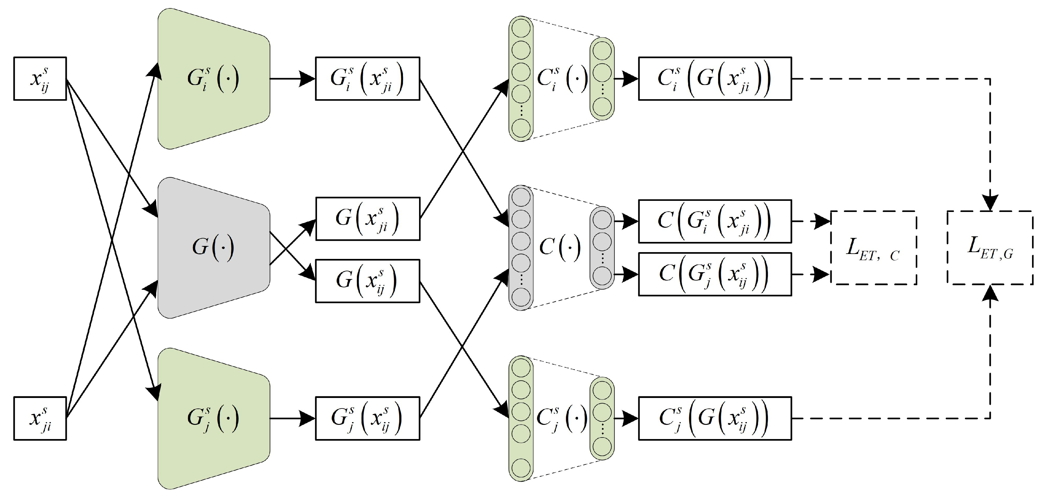
2.2. The Proposed Method
As illustrated in
Figure 1, in the proposed episodic training and feature orthogonality driven domain generalization (EODG) method, the general feature extractor
and general fault classifier
are combined to create the final DGFD model
, whereas the domain classification model
that consists of a domain feature extractor
and domain classifier
and the domain-specific fault diagnosis model
that consists of domain-specific feature extractors
and domain-specific fault classifiers
are used to facilitate the learning of domain-invariant fault diagnosis knowledge. The learning procedure of EODG consists of three parts: (1) supervised learning; (2) domain-invariant representation learning; (3) episodic training. Supervised learning aims to enable the DGFD model, domain-specific fault diagnosis models, and the domain classification model to complete their respective fundamental tasks effectively. In addition, domain-invariant representation learning aims to enable
to extract domain-invariant features. Finally, episodic training is applied to enhance the generalization capabilities of both
and
.
2.2.1. Supervise Learning
Supervised learning is applied to train these models to acquire basic abilities on their respective classification tasks. Via supervised learning, learns to extract fault-related features across multiple source domains, learns to diagnose the health conditions of machinery in these domains, learns to extract domain-related features from multiple source-domain data, learns to classify their domain label, learns to extract fault-related features from specific source domains, and learns to diagnose the health conditions of machinery in specific source domains.
In this study, cross-entropy loss is used for all supervised learning tasks; supervised learning loss for the DGFD model
, the domain classification model
, and the domain-specific fault diagnosis model
is defined as follows:
where
is the number of source domains;
is the fault label of the source-domain sample
;
is the output of the DGFD model;
is the domain label of the source-domain sample
;
is the output of the domain classification model;
is the fault label of the
i-th source-domain sample
, and
is the output of the
i-th source-domain-specific model.
2.2.2. Domain-Invariant Representation Learning
In EODG, feature orthogonalization constraint and feature transfer loss are combined to learn domain-invariant representations. Feature orthogonalization encourages orthogonality between fault-related and domain-related features by minimizing their cosine similarity. To align the feature distribution of same-class samples across different domains, and to separate the feature distribution of different-class samples, a novel feature transfer loss is proposed based on MMD in this paper [
32]. The feature orthogonalization loss
and feature transfer loss
are defined as follows:
where
represents the cosine similarity function;
represents the maximum mean discrepancy function;
and
represent the features of dataset
and
, respectively;
and
contain all
c-th-category samples that belong to the
i-th source domain and the
j-th source domain, respectively;
represents the features set of dataset
, which contains all samples belonging to the
c-th category;
represents the center of
, which is the feature center of the
c-th category;
is the feature center of all samples;
,
,
, and
,
represent the number of categories.
It can be seen from Equation (5) that by minimizing , the feature distributions of samples that have the same fault label but different domain labels are aligned, and all feature distributions of same-class samples are aligned with their feature center; meanwhile, the feature distributions of different categories are separated, and the feature distributions of each category are separated from the feature center of all samples.
2.2.3. Episodic Training
Most existing DGFD methods focus on training feature extractors to extract domain-invariant features, while the generalization capability of the fault classifier is overlooked. In EODG, episodic training [
33] is applied to improve the generalization capabilities of both the general feature extractor
and the general fault classifier
. In episodic training, general modules and domain-specific modules are combined to form hybrid models which are trained in a supervised learning manner. As shown in
Figure 2, in the case of the two source domains, the
i-th and
j-th domain-specific feature extractors are combined with the general fault classifier to form hybrid models
and
, respectively; meanwhile, the
i-th and
j-th domain-specific fault classifiers are combined with a general feature extractor to form hybrid models
and
. Then, labeled samples from other domains are used for the supervised training of each domain-specific hybrid model. Finally, the trained
is able to extract general features from samples of other domains which can be classified by the domain-specific fault classifier, and the trained
is able to classify the features extracted by the domain-specific feature extractor. Therefore, the generalization capabilities of
and
are effectively improved.
To meet the requirements of a heterogeneous DGFD setting, only shared-category samples from other domains are used for the supervised training of each domain-specific hybrid model in EODG. The loss of episodic training is defined as follows:
where
is the sample of the
i-th source domain that comes from the shared categories between
i-th and
j-th source domains, and
is the fault label of
,
,
.
2.3. Diagnosis Procedures
In EODG, supervised learning, domain-invariant representation learning and episodic training are used for model training. During the training procedure, the losses for the general feature extractor
, the general fault classifier
, the domain feature extractor
, the domain classifier
, domain-specific feature extractors
and domain-specific fault classifiers
are defined as follows:
where
,
, and
are tradeoff parameters.
The procedures of the proposed EODG method are presented in
Figure 3, and summarized as follows:
Step 1: Collect vibration signals from rotating machinery and partition them into labeled source-domain signals for model training and unseen target-domain signals for model evaluation. Then, segment and standardize these signals to form labeled source-domain datasets and testing datasets .
Step 2: Construct a general feature extractor , a general fault classifier , a domain feature extractor , a domain classifier , domain-specific feature extractors and domain-specific fault classifiers . Pre-train these modules via supervised learning.
Step 3: Sample a batch of training data from . Train and . Then, freeze the parameters of and , and train , , and .
Step 4: Repeat Step 3 until the labeled source-domain dataset is traversed.
Step 5: Repeat Step 3 to Step 4 until the preset maximum number of epochs is reached.
3. Experimental Study
3.1. Datasets Description
In this study, a well-known public HUST bearing dataset and a CNC bearing dataset are used for the verification of the proposed method. Detailed descriptions of these datasets are provided below.
3.1.1. Huazhong University of Science and Technology (HUST) Bearing Dataset
The HUST bearing dataset was provided by Zhao et al. [
34]. The test rig of this dataset is shown in
Figure 4, and it consists of the following: 1. speed control; 2. a motor; 3. a shaft; 4. an accelerometer; 5. a bearing; and 6. a data acquisition board.
This dataset contains a normal state and four types of failure state, and each failure state has two severity levels. Vibration signals are collected at a sampling rate of 25.6 kHz. The data on the five types of health state (normal, inner-race fault, outer-race fault, ball fault, and inner- and outer-race combination fault) under six rotating speeds (20 Hz, 25 Hz, 30 Hz, 35 Hz, 40 Hz, and varying speeds (0–40–0 Hz)) are selected to evaluate the proposed method. The details of the HUST bearing dataset are listed in
Table 1.
The test bearing used in the HUST dataset is a deep groove ball bearing, Rexnord ER16K, and its detailed specifications are listed in
Table 2.
3.1.2. CNC Bearing Dataset
The test rig of the CNC bearing dataset is shown in
Figure 5. The spindle of CNC is supported by four rolling bearings, and four types of faults (inner-race fault, outer-race fault, and cage fault) are introduced to the third bearing (marked in red). The experimental setup involved cutting aluminum materials under seven spindle speeds, with a feed rate of 2500 mm/min, a cutting depth of 0.1 mm, and a cutting width of 3 mm. Vibration data were acquired using an accelerometer mounted on the bearing housing with a sampling rate of 25.6 kHz. The details of the CNC bearing dataset are listed in
Table 3.
The test bearing used in the CNC dataset is an angular contact ball bearing, NSK 40BNR10, and its detailed specifications are listed in
Table 4.
3.2. Implementation Details
3.2.1. Network Structure and Hyperparameters
The network structures of the general feature extractor
, the general fault classifier
, the domain feature extractor
, the domain classifier
, domain-specific feature extractors
and domain-specific fault classifiers
are listed in
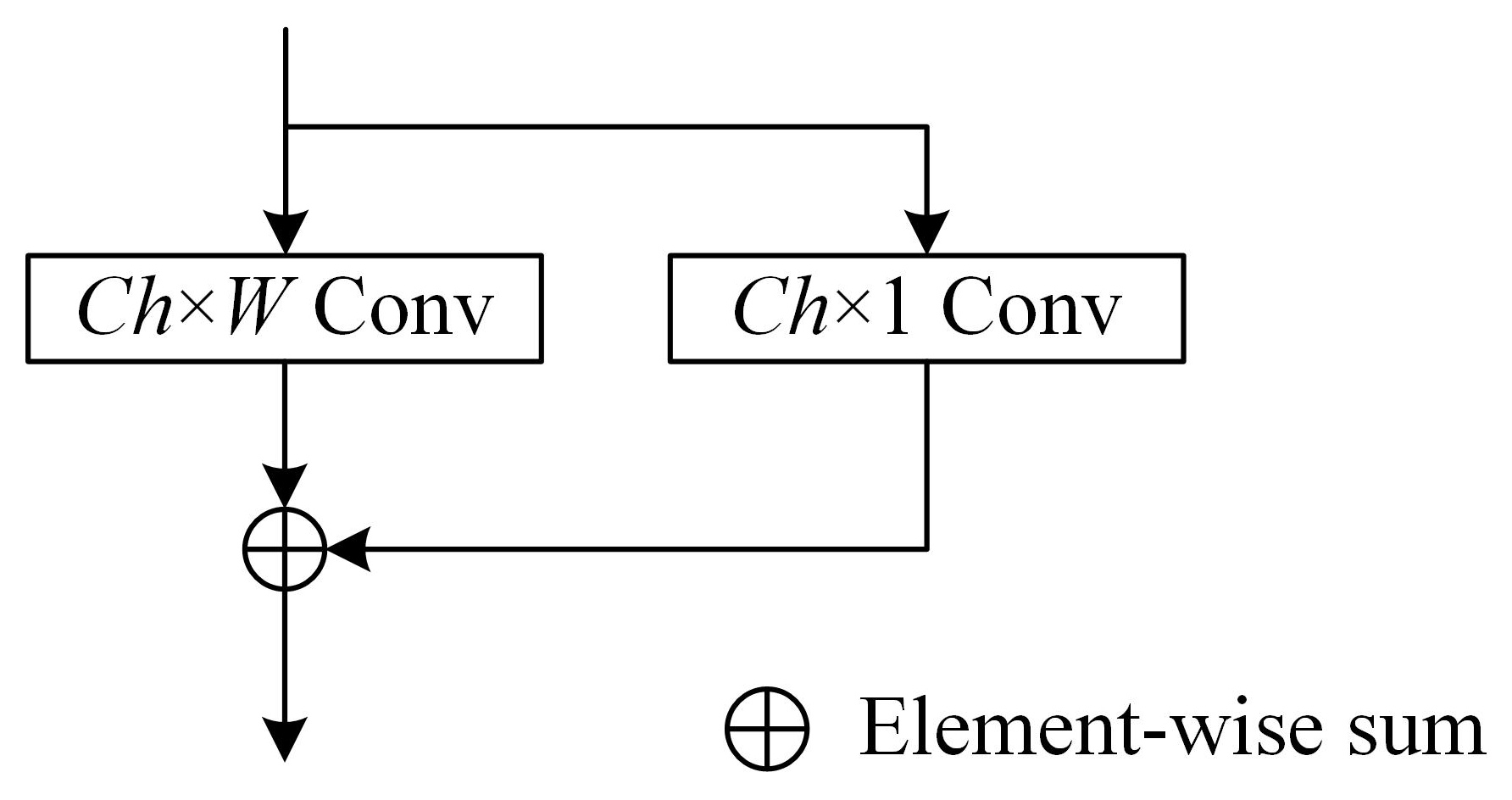
Table 5. The structure of ResBlock is shown in
Figure 6, where
Ch represents the output channel, and
W represents the convolutional kernel size.
As can be seen from
Table 3,
,
, and
share the same network structure. The distinction between
,
, and
lies in their output layers, where the output sizes of
and
are determined by the number of classes
, and the output size of
is determined by the number of source domains
.
In this study, the negative slope of Leaky_ReLU is set as 0.1, and the Adam optimizer is used for training with a learning rate of 0.004. The model is trained using a batch size of 64 for 128 epochs. The tradeoff parameters are set as follows: , , and .
3.2.2. Experimental Setting
To evaluate the effectiveness of the proposed method, the HUST bearing dataset and CNC bearing dataset are used for multiple-source-domain generalization fault diagnosis experiments; the details of the experimental settings used are listed in
Table 6 and
Table 7, respectively. In this paper, the domain shifts between source and target domains arise from variations in rotating speed, which are directly proportional to the fault characteristics frequency. In the HUST bearing dataset, each category has 100 samples, with a sample length of 2048 data points. In CNC bearing datasets, each category has 200 samples, with the sample length of 2048 data points.
For each task, three speeds are randomly selected, and the corresponding domains are designated as source domains, whereas the remaining domains serve as target domains. To fulfill the requirements of a heterogeneous setting, the fault types differ across source domains. Specifically, all domains contain the normal state, as it is easy to achieve. In addition, each target fault type is required to appear in at least two different source domains, to learn consistent representations across domains. To verify the model’s DGFD performance for each fault type, all target domains share the same fault types, which cover all fault types that have occurred in the source domains.
Datasets of each domain are identified by their working conditions and fault categories. In
Table 4, the working condition is represented by the rotating speed in units of Hz, where 20 denotes 20 Hz, 25 denotes 25 Hz, and so on. Specifically, VS denotes varying speed (0-40-0 Hz). The definitions of the fault codes can be found by referring to
Table 1. In
Table 5, the working condition is represented by the spindle rotation speed in units of rpm, where 6k denotes 6000 rpm, 7k denotes 7000 rpm, etc. The definitions of the fault codes are listed in
Table 2. The dataset pertaining to the first source domain (S1) of the first HUST task (H1) is represented by 20 (H IRF BF ComF), where 20 indicates that the test rig is operating at a speed of 20 Hz, and (N IRF BF ComF) refers to the inclusion of four types of data (normal, inner-race fault, ball fault, and inner- and outer-race fault). For target domains, all datasets shared the same fault categories, and these datasets are uniformly represented, such as the datasets of target domains of H1, which is represented by 35 40 VS (N IRF ORF BF ComF), where 35 40 VS indicates the rotating speeds of the three target domains, each containing five types of data (normal, inner-race fault, outer-race fault, ball fault, and inner- and outer-race fault).
3.3. Benchmarked Approaches
To evaluate the effectiveness of the proposed methods, five methods are used for comparison.
(1) Convolutional Neural Networks (CNNs): All source-domain datasets are combined and used to train the model in a supervised learning manner.
(2) Conditional generative adversarial networks (CGANs) [
21]: CGANs use a discriminator that can simultaneously classify the fault type and domain label for domain-adversarial training.
(3) Adversarial-Domain-Invariant Generalization (ADIG) [
22]: In ADIG, the reshaped two-dimensional frequency spectrum is used as the input of the model, and adversarial learning and feature normalization strategies are leveraged to learn domain-invariant knowledge.
(4) Conditional Contrastive Domain Generalization (CCDG) [
23]: CCDG uses mutual information to capture shareable fault information and learn domain-independent representations for rotary machine fault diagnosis in unseen domains.
(5) Causal Consistency Networks (CCNs) [
24]: CCNs use the proposed causal consistency loss and collaborative training loss to learn consistent causality knowledge for bearing domain generalization fault diagnosis.
3.4. Results and Discussion
In this study, all experiments were implemented on an NVIDIA TITAN V GPU (Nvidia Corporation, Santa Clara, CA, USA) with the Pytorch 2.6.0 framework. The diagnostic accuracy, defined as the ratio of the number of correctly predicted test samples to the total number of test samples, is adopted as the evaluation metric. Each task is repeated ten times to reduce randomness.
3.4.1. Experimental Results of HUST Bearing Dataset
The diagnosis results of the HUST bearing dataset are presented in
Table 8, which includes the mean and standard deviation of the accuracies of ten trials for each task. Specifically, the final row (Avg.) shows the average performance across all tasks. To further illustrate these results,
Figure 7 shows the accuracy curve of each target domain, along with the average accuracy curve of all target domains, while
Figure 8 presents a histogram of the diagnostic accuracy and corresponding standard deviations.
CNN achieves the lowest overall accuracy of 73.06%, which reveals the limitations of traditional supervised learning while applied to DGFD tasks. Among the DGFD methods, CGANs and ADIG are adversarial methods, and CCDG, CCNs and the proposed EODG method are non-adversarial methods. ADIG achieves the second highest overall accuracy of 83.74%, significantly outperforming CGANs, CCDG and CCNs. The superior performance of ADIG over that of CGANs indicates that incorporating frequency-spectrum inputs and feature normalization strategies can enhance generalization.
Among these methods, the proposed EODG method achieves the highest overall accuracy of 87.47%, outperforming all other benchmark methods. EODG consistently achieves superior performance across nearly all tasks and achieves the highest overall accuracy. The only exception is Task H2, where its accuracy (80.65%) is marginally lower (by 0.55%) than the best-performing method (ADIG, 81.20%). As illustrated in
Figure 7, EODG demonstrates consistently strong performance across individual target domains.
Figure 8 shows that EODG achieved the best overall performance with relatively small standard deviations.
In summary, the results of HUST bearing datasets demonstrate the effectiveness and superiority of the proposed EODG method in DGFD tasks. The combination of episodic training (EPI), feature transfer (FT) constraint and feature orthogonalization (FO) constraint can significantly improve the generalization of intelligent fault diagnosis model.
3.4.2. Experimental Results of CNC Bearing Dataset
The results of the CNC bearing datasets are shown in
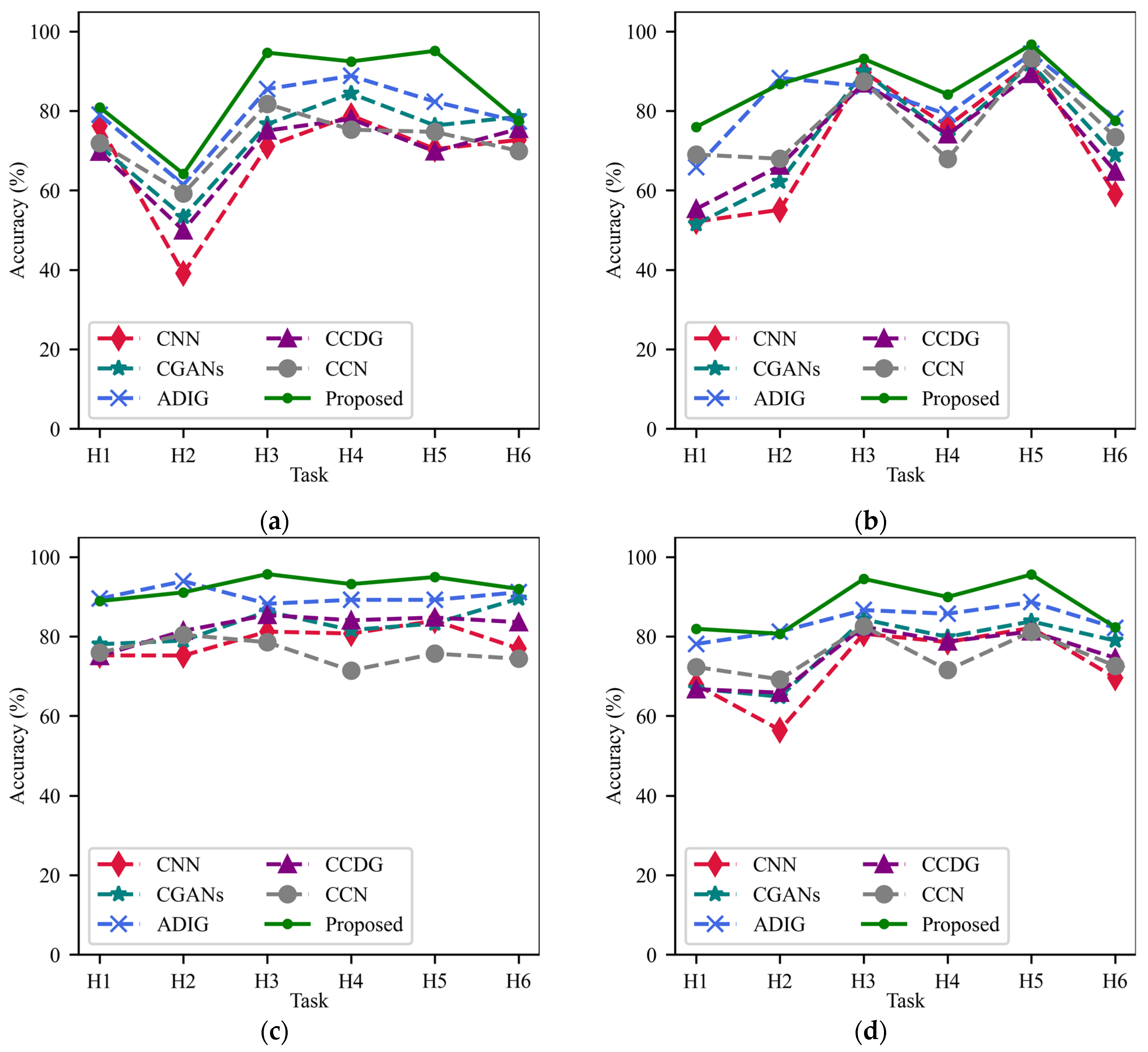
Table 9, and they are similar to the results of the HUST bearing datasets: CNNs achieve the lowest overall accuracy of 70.84%. The overall accuracies of CGANs, CCDG and CCNs are close, all slightly outperforming that of CNNs. ADIG achieves the second highest overall accuracy of 80.88%. In some tasks, ADIG shows higher accuracy than the proposed EODG method.
EODG achieves the highest overall accuracy of 85.56%, significantly outperforming other methods. EODG achieves the highest accuracy in most individual tasks, except C3, C5, and C6, in which its accuracy falls short of the best-performing method by no more than 1.5%.
Figure 9 and
Figure 10 show the accuracy curves and histogram of the experimental results, respectively. In these figures, the EODG method shows the best diagnosis performance in most individual target domains and shows the best overall performance with relatively small standard deviations, demonstrating the effectiveness, superiority and robustness of the proposed method.
3.5. Feature Visualization
To further evaluate the effectiveness of the proposed method, t-distributed stochastic neighbor embedding (t-SNE) is used for feature visualization [
35]. Because the output features of the feature extractor are used for domain-invariant representation learning for all methods except CNNs, feature visualization is conducted on these features. Task C7 is selected for the visualization.
Figure 11 presents the results of feature visualization, where the legend consists of the fault label and the domain label. For example, “IFR(T)” represents that the inner-race fault samples from the target domain. It can be seen from
Figure 11 that CNNs, CGANs, and CCNs exhibit category confusion in the extracted features. ADIG exhibits good inter-class discrimination, with almost no category confusion. However, its inter-domain integration is poor, as few target-domain samples are integrated with the corresponding source-domain samples of the same category. CCDG shows good inter-class discrimination and better inter-domain integration than ADIG. Among these methods, EODG exhibits the best domain-invariant feature extraction ability, with clear inter-class boundaries and excellent inter-domain integration. The target-domain samples are clustered near the corresponding source-domain samples of the same category.
The feature visualization results demonstrate that EODG can effectively extract domain-invariant features, even in the presence of unseen working conditions.
3.6. Ablation Study
In this section, the influences of FO, EPI, and FT on the performance of the model are analyzed. Six variants of EODG are used for the ablation study: (1) FO: the model is trained with supervised learning and feature orthogonalization constraint; (2) EPI: the model is trained with supervised learning and episodic training; (3) FT: the model is trained with supervised learning and feature transfer constraint; (4) EPI + FO: the model is trained with supervised learning, episodic training, and feature orthogonalization constraint; (5) FT + FO: the model is trained with supervised learning, feature transfer constraint, and feature orthogonalization constraint; (6) FT + EPI: the model is trained with supervised learning, feature transfer constraint, and episodic training.
The results of the ablation study are listed in
Table 10 and shown in
Figure 12. The results demonstrate that the contribution ranking is FT (78.47%) > EPI (76.76%) > FO (74.70%). The combination of FT and EPI achieves the second highest overall accuracy of 79.45%, which is higher than that of the individual EPI and FT variants. For EPI + FO, it also achieves higher overall accuracy than EPI and FO. FT + FO performs slightly better than FO, but slightly worse than FT. EODG with a combination of FO, EPI and FT outperforms all six variants in all individual tasks, which demonstrates the effectiveness of this combination.
In
Figure 12, EODG shows the highest accuracy in every task and the smallest standard deviation in almost all tasks. The results of the ablation study demonstrate that FO, EPI and FT can effectively improve the generalization of the DGFD model. Furthermore, FT gives model the basic ability to perform DGFD by learning domain-invariant representations, while the additions of EPI and FO further boost the DGFD performance of the intelligent fault diagnosis model. In the practical industry, rotating machinery is always required to operate under varying working conditions. The proposed EODG method can train a DGFD model that can mitigate the performance degradation caused by changes in working conditions, thereby broadening the applications of intelligent fault diagnosis methods in practical industry.


 ,
, 


