Application of Artificial Neural Networks in Predicting Surface Quality and Machining Time

Abstract

This paper explores the use of artificial neural networks to optimize metal machining processes. It has two main components. The first component focuses on developing a neural network in EasyNN to predict quality errors of metal surfaces machined with toroidal milling. The input data are extracted from the experimental values of the machining operations, and the output data are the measured surface roughness values. The network created not only predicts the quality errors but also identifies the key parameters influencing their quality, such as cutting speed, feed rate, and tool geometry, which are crucial for process optimization. The second component underscores the accuracy of the neural network′s predictions by using MatLab to develop a neural network that estimates the machining time, a key factor in cost calculation and efficient order planning. The experimental data used to train the network come from a restricted set of machining jobs. The obtained results demonstrate an adequate estimation of the machining time, thus facilitating the optimization of the entire metal machining process, positively impacting the cost and efficiency of industrial operations.

1. Introduction

We hear more and more about artificial intelligence, software that can answer certain questions, and applications that help mankind by allowing us to understand and link information. All these software are based on artificial neural networks, where artificial intelligence manages to provide answers through a computational algorithm, through tens, hundreds, thousands, and millions of hidden neurons [1,2].

If we consider the level of continuous development of cutting surface machining, new technologies, optimizations, tools, machines, software, and precision measuring instruments, we consider the involvement of artificial neural networks in machining to be more than necessary.

The application of artificial neural networks in cutting process performance improvement has been extensively studied in different research [3,4]. These studies, along with the prediction of machined surface quality and output quality, demonstrate the practicality and applicability of these tools [5,6]. Other approaches of artificial neural networks in machining process improvement have been applied in the study of cutting tool wear [7] as well as the study of cutting forces [8,9]. These practical applications of artificial neural networks in the field of machining instill confidence in their effectiveness and utility.

Implementing artificial neural networks for surface quality monitoring [10] or tool wear monitoring [11] in chip machining by either milling or turning offers a wealth of opportunities, leading to lower production costs.

EasyNN plus, a specialized software for building and using neural networks, played a crucial role in this research. It provided a user-friendly graphical user interface and multiple facilities related to network manipulation, making it an ideal tool for our study.

According to Boujelbene et al., milling operation is the most important and widely used technology for obtaining complex surfaces. A computer numerically controlled (CNC) milling machine and CAD/CAM software (PowerMILL 2015) capable of realizing an NC program are needed to perform this operation. In this process, the machine should move as fast as possible with well-defined trajectories according to the cutting tool typology [12]. The optimization of milling operations is always a hot topic in manufacturing because the ability to carry out machining processes at maximum performance is irreplaceable in increasing production efficiency. However, obtaining reliable and practicable solutions is still challenging for milling operations [13].

The actual machining time depends on the CNC, dynamic machine architecture, setup times, space ergonomics, and their implementation, as well as the CAM software used [14].

Current CAD/CAM software estimates the milling time mathematically by dividing the tool path length by the user-set feed rate value, excluding the machining limitation and the machine/CNC feed rate oscillation. This approach, however, does not account for the actual conditions of the machining process, leading to inaccurate estimates. For these reasons, the CAM-estimated time is not the correct one. As a result, in this paper, we will only summarize the basic time.

Some authors have proposed artificial neural networks for feature recognition [15] to further establish relationships between the number of features and part cost [16].

Other authors have presented models using artificial intelligence to estimate machining time with average errors of 10 and 20 min [17] or manufacturing time with a percentage error of less than 25% [18]. Artificial intelligence tools for estimating manufacturing costs in the design phase have also been studied [19,20,21,22], as well as the effectiveness of different types of ANNs in estimating machining times [23,24,25,26,27].

The main goal of this work is to develop and validate a model based on artificial neural networks, capable of providing a fast and accurate estimation of machining times and the quality of surface for industrial parts. This approach is intended to be a viable and efficient alternative to the traditional simulation methods used in CAM software, methods that, although accurate, involve a significant consumption of time and resources.

The overall objective is to create an intelligent tool that supports companies in the field of machining in optimizing production processes, by reducing the time needed to estimate costs and delivery times. In this regard, the proposed neural network will allow the automatic and real-time deduction of processing times and surface quality, thus providing valuable decision-making support in the bidding, planning and execution phases of orders.

2. Materials and Methods

The present paper aims to investigate the applicability of artificial neural networks in two essential directions for the machining industry: on the one hand, the prediction of surface quality by estimating roughness in the case of flat surfaces, and on the other hand, the estimation of execution times in the machining process of concave cylindrical surfaces.

The choice of these two characteristics—surface quality and process duration—reflects the current requirements of the economic environment, which aims to achieve high-quality finishes in the shortest possible manufacturing time. The simultaneous fulfillment of these objectives leads, implicitly, to the reduction in production costs and to the observance of delivery deadlines, essential aspects for the competitiveness of companies.

Regarding the approach of the two types of surfaces analyzed in this work, the high potential of artificial neural networks to be applied in a wide range of contexts is highlighted, while also being able to work in parallel in any circumstances.

2.1. Experimental Research on Flat Surface Processing with Toroidal Milling Cutter

The experimental investigation that underpinned this study was detailed in previously published papers [2], aiming to collect the input and output data needed to train the artificial neural network. As for the practical experiment, it consisted of processing 27 test samples on a five-axis CNC machining center, model Okuma MU-400VA from Okuma Deutschland GmbH from Köln, Germany. (Figure 1A).

The number of samples was established based on the Taguchi method, using the minimum number of tests necessary to obtain statistically relevant results.

Geometrically, each specimen had dimensions of 40 × 40 × 20 mm³. The finishing operation was carried out on a flat and rough surface, with the pieces being fixed in a vice with the help of a special clamping device.

The finishing machining was performed with a toroidal milling cutter with a diameter of Ø16 and a corner radius of 4 (Figure 1B) in the presence of the cutting liquid. The cutting liquid, which is a coolant and lubricant, helps to reduce heat and friction during the machining process, thereby improving the surface quality. The machining was carried out with a constant chip depth (ap = 0.5 mm) and radial depth (ae = 0.3 mm) (Figure 2b).

The CAM program was generated in the PowerMILL software (Figure 2a), which can generate the tool paths by respecting the required machining regimes and the transmitted inclination angle.

In order to execute the processing of the 27 surfaces included in the scope of this study, the experimental framework was designed in accordance with the Taguchi method, as described in detail in prior research. This method provides a robust and systematic approach for optimizing process parameters by minimizing variability and identifying the most influential factors with a reduced number of experimental runs. Based on this framework, it was established that a portion of the cutting regime parameters would be held constant throughout the experimentation. This decision was made to ensure consistency and control over extraneous variables, thereby isolating the effects of the key parameters under investigation. The specific values and constraints of these constant parameters were defined in alignment with the technical specifications and machining conditions presented earlier.

In parallel, three primary technological parameters were selected to serve as variable inputs for the development and training of the artificial neural network (ANN) model proposed in this study. These input variables, as listed in

Table 1. Cutting regimes and measured roughness values.

Experiment	Cutting Speed [m/min]	Angle of Inclination [°]	Feed Per Tooth [mm/tooth]	Ra Parallel [µm]	Rt Parallel [µm]	Ra Perpendicular [µm]	Rt Perpendicular [µm]
SPLN-TR-1	80	15	0.11	0.16	0.926	0.464	2.92
SPLN-TR-2	80	15	0.15	0.289	1.68	0.403	2.593
SPLN-TR-3	80	15	0.19	0.264	1.706	0.376	2.4
SPLN-TR-4	80	35	0.11	0.194	1.466	0.494	2.613
SPLN-TR-5	80	35	0.15	0.311	2.413	0.435	3.499
SPLN-TR-6	80	35	0.19	0.288	2.719	0.425	2.953
SPLN-TR-7	80	55	0.11	0.45	2.609	0.688	4.273
SPLN-TR-8	80	55	0.15	0.727	4.413	0.632	4.353
SPLN-TR-9	80	55	0.19	0.894	4.639	0.761	5.84
SPLN-TR-10	170	15	0.11	0.689	3.486	0.672	4.519
SPLN-TR-11	170	15	0.15	0.817	4.646	0.756	5.406
SPLN-TR-12	170	15	0.19	0.876	5.094	0.851	6.086
SPLN-TR-13	170	35	0.11	0.597	3.247	0.786	5.579
SPLN-TR-14	170	35	0.15	0.693	3.906	0.805	4.826
SPLN-TR-15	170	35	0.19	1.071	5.76	1.119	7.666
SPLN-TR-16	170	55	0.11	0.457	3.273	0.535	3.619
SPLN-TR-17	170	55	0.15	0.773	4.306	0.627	5.106
SPLN-TR-18	170	55	0.19	1.131	6.103	0.812	6.293
SPLN-TR-19	210	15	0.11	0.53	3.786	0.549	4.053
SPLN-TR-20	210	15	0.15	0.859	4.833	0.757	4.759
SPLN-TR-21	210	15	0.19	0.893	4.799	0.869	6.326
SPLN-TR-22	210	35	0.11	0.568	3.899	0.543	4.146
SPLN-TR-23	210	35	0.15	0.598	3.753	0.573	4.496
SPLN-TR-24	210	35	0.19	0.513	2.966	0.618	4.586
SPLN-TR-25	210	55	0.11	0.402	3.552	0.445	3.7
SPLN-TR-26	210	55	0.15	0.402	2.993	0.475	3.853
SPLN-TR-27	210	55	0.19	0.423	3.186	0.596	4.56

, are cutting speed, tool tilt angle, and feed per tooth. The selection of these particular variables was guided by both theoretical and empirical considerations. From a theoretical standpoint, these parameters are known to play a decisive role in determining machining outcomes, particularly with respect to surface integrity and overall process efficiency. Empirical evidence from previous investigations further supports their significant influence on surface roughness, dimensional accuracy, material removal rate, and tool wear.

By incorporating these three variables into the ANN model, the objective is to enable a predictive framework capable of capturing the nonlinear relationships between input parameters and machining responses. Their selection reflects a deliberate focus on optimizing both surface quality and processing time, two of the most critical performance indicators in modern manufacturing environments. The ANN′s ability to model these complex interdependencies is expected to provide valuable insights for process optimization and decision-making in advanced machining applications.

2.2. Experimental Research on the Machining of Concave Cylindrical Surfaces with Toroidal Milling Cutter

Our analysis of the concave cylindrical surface reveals a consistent cylindrical shape along the entire length of the surface. The surface, with a diameter of Ø85 and a height of 5 mm, measures 40 × 40 mm², as shown in Figure 3. The practical experiments on the concave cylindrical surface are presented in

Table 2. Run time for machining concave cylindrical surfaces with toroidal milling cutter.

Experiment	Cutting Speed [m/min]	Angle of Inclination [°]	Feed Per Tooth [mm/tooth]	Execution Time [s]
CICV-TR-1	80	55°	0.11	964
CICV-TR-2	80	55°	0.15	734
CICV-TR-3	80	55°	0.19	601
CICV-TR-4	170	55°	0.11	508
CICV-TR-5	170	55°	0.15	399
CICV-TR-6	170	55°	0.19	337
CICV-TR-7	210	55°	0.11	430
CICV-TR-8	210	55°	0.15	343
CICV-TR-9	210	55°	0.19	292

, which details nine surfaces, each created using toroidal milling. The table includes a column highlighting the execution times of each experiment, excluding the constant auxiliary times, to provide a clear comparison of the experiments.

Regarding the cutting regimes, the three variables in the table (Table 2) are the focus, while the rest remain constant. The cutting depth is consistently set at 0.5 mm (ap = 0.5 mm) and the radial depth at 0.3 mm (ae = 0.3 mm) for each experiment, all conducted in the presence of emulsion, which serves as a crucial element in the process. As for the clamping method, the pad is securely clamped between the two clamping trays of the vice, which are further reinforced with clamping for extra rigidity and security.

In order to be able to carry out the machining, CAM programs are needed; they were created using the PowerMILL software, a software able to create the tool, and more importantly, to create the routes to be covered by the tool with the corresponding inputs and outputs. We decided that each machining would be one-way, with the tool paths parallel. For machining the surface with the toroidal milling cutter, in the case of the 55° inclination, 138 lines were needed. Figure 4a shows an image during the simulation of the toroidal toolpath on the concave cylindrical surface.

Figure 4b presents the actual practical experiment conducted on the OKUMA MU-400VA CNC. This figure vividly demonstrates how the toroidal milling cutter effectively processes the concave cylindrical surface, providing a tangible application of the theoretical concepts discussed.

It is important to note that throughout the machining of the concave cylindrical surface with the toroidal milling cutter, the tool axis constantly maintains the desired inclination angle concerning the surface.

Experimental Results

Following the processing and simulation in CAM software, different processing times resulted during the realization of the nine surfaces with different regimes, as presented in Table 2.

3. Results and Discussion

3.1. Implementing the Artificial Neural Network in EasyNN

An example of a neural network constructed utilizing EasyNN software is presented below. A neural network must be constructed to predict the roughness values Ra, measured both in parallel and perpendicularly, as well as the roughness Rt, also measured in both orientations.

The data input is a critical step in the process. The input data consists of the cutting speed, the feed per tooth, and the feed angle, which are the three variables utilized to machine each SPLN-TR surface. The output data are characterized by the roughness measurements taken in both parallel and perpendicular orientations to the feed direction. These measurements are denoted as the theoretical surface roughness, Rt, and the arithmetic mean roughness, Ra.

The database depicted in Figure 5 is structured as a data grid. The rows correspond to the examples, while the columns denote the inputs and outputs associated with each example. The initial column specifies the type and designation of the input and output example. The subsequent three columns denote the three process variables that are being materialized as input data, while the final four columns indicate the measured values of roughness, representing the output data.

After loading the database, the subsequent step involves verifying the usability of the data via the “Query” function, followed by the establishment of the neural network.

The neural network is established using the previously loaded data grid. This process is initiated through the “new network” function, which generates the new network dialog. This dialog facilitates the specification of the neural network configuration, enabling it to learn information from the database.

The learning progress indicates the advancement of the learning process. Figure 6 illustrates the learning process graph, which displays the maximum, average, and minimum training error values. The graph progressively narrows as learning advances, ensuring visibility of the complete learning curve. A maximum of 200,000,000 learning cycles can be represented in the graph; however, in this instance, only 3873 learning cycles are required.

Figure 6 displays a vertical scale on the left side, ranging from 0 to 1, which indicates the position of the curve. The horizontal scale is labeled in accordance with the quantity of the learning cycles.

Below the horizontal scale, the network is displayed, indicating the number of inputs, outputs, and hidden neurons. In this instance, a variant with 10 hidden neurons has been selected. The window displays the quantity of connections among nodes, specifically 30 connections between the input layer and the hidden layer, and 40 connections between the hidden layer and the output neurons.

The right side of the graph displays the window containing the learning and validation data. The learning rate is configured at 0.5, the momentum is established at 0.8, and the training process is programmed to terminate when the error threshold reaches 0.15. The recorded maximum error is 0.01492259, while the minimum error is 0.000024. The average of the errors is calculated to be 0.0376863.

Upon completion of the settings, the configuration of the analyzed neural network is illustrated in Figure 7.

To utilize the neural network effectively, it is essential to select the source and destination of the connections for the purpose of connecting and disconnecting the nodes. Connections can be established between any nodes or layers, allowing for flexible integration across the system. Feedback and layer-level connections are feasible.

The quantity of nodes within hidden layers may be adjusted, and additional hidden layers can be incorporated as required. The nodes will be reestablished utilizing the connections stored in the network′s memory. The connections will be maintained in a manner that closely resembles their prior configuration.

3.2. Implementing the Artificial Neural Network in MATLAB

Neural networks primarily function by identifying a relationship that links the output parameters to the input parameters. Throughout the training process. Upon completion of the training process, the neural network demonstrates functionality in scenarios that were not part of the training dataset.

Cutting parameters represent critical factors that significantly impact process plans. The optimal selection of cutting parameters results in a decrease in cutting actions, which subsequently leads to reduced energy consumption and, consequently, cost reduction. This study aims to implement cutting parameter prediction through the utilization of artificial neural networks (ANNs). Neural networks are widely utilized tools that have demonstrated effectiveness in addressing optimization problems, particularly in the adaptive control of machine tools and in pattern recognition applications.

The MATLAB R2015a program includes a set of functions and graphical interfaces designed for the manipulation of Artificial Neural Networks, collectively referred to as the Neural Network Toolbox. The subsequent sections will outline the methodology for utilizing the basic functions and interacting with the graphic interfaces.

Prior to the development of an artificial neural network, it is essential to establish the input data and the output data. The computer resources outlined in the preceding chapter are applicable in this context.

In order to generate the input and output data, we selected to analyze the fundamental time derived from the processing of nine cylindrical-concave specimens using the toroidal milling cutter. Consequently, the two process variables are identified as input data, specifically the cutting speed and the feed per tooth. The output data and target information are represented by the fundamental time required to process each surface.

The artificial neural network was developed in the MATLAB environment, using the input and output data presented above. The structure of the network comprises two layers and was trained using the TRAINLM (Levenberg–Marquardt) algorithm, known for its efficiency in regression problems. For the hidden layer, 10 neurons were chosen, a choice made after preliminary tests to ensure a balance between complexity and generalization capacity.

In terms of network performance, the training process ended after three epochs with the network reaching a satisfactory level of convergence. The dataset was divided as follows: about 77% of the data was allocated for training and 11% each was used for validation and testing for the purpose of evaluating the robustness and accuracy of the model.

The first step in generating a neural network consists of providing the input and output data necessary for the artificial neural network to train and learn, a process presented in Appendix A.

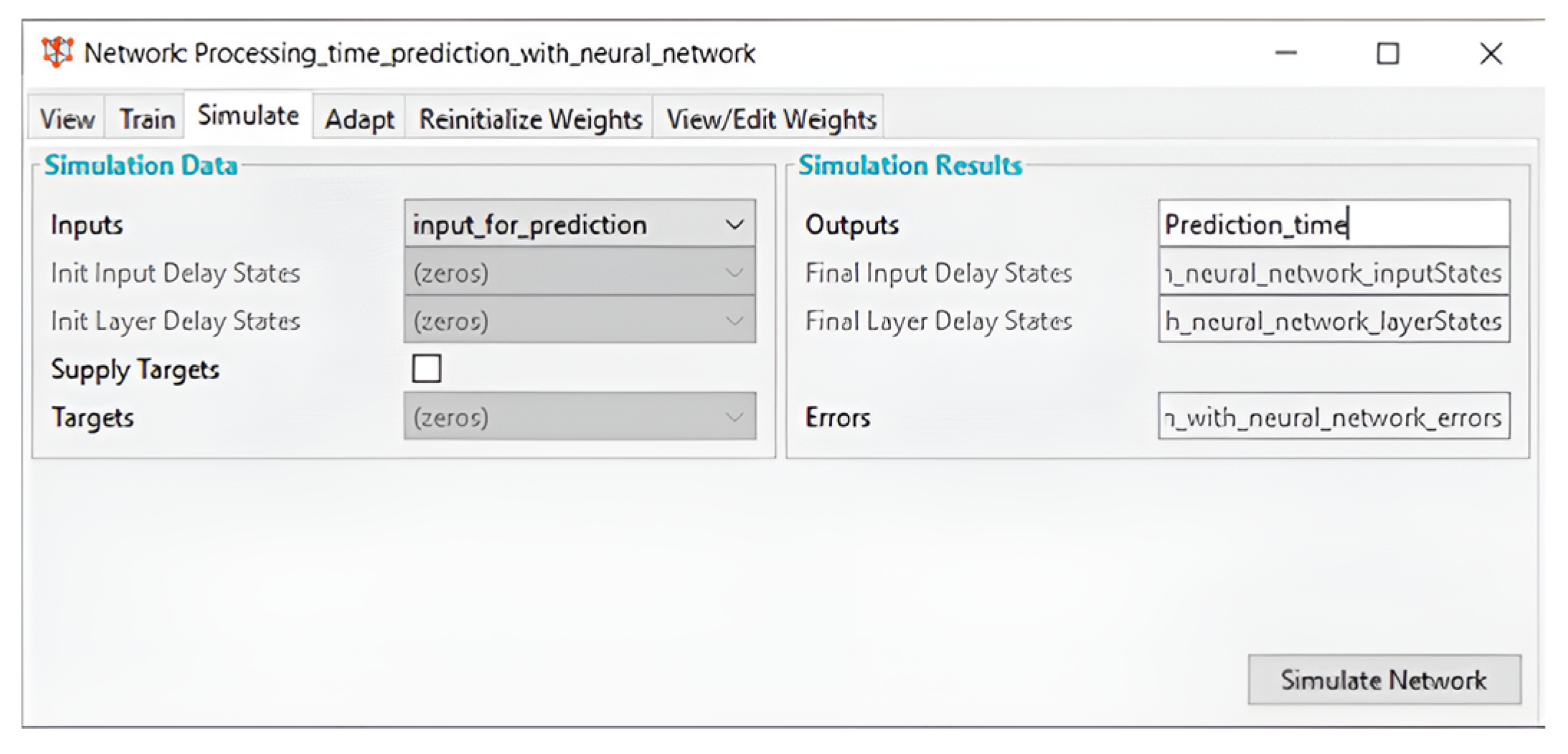
Upon completion of the training and learning phase of the artificial neural network, the subsequent stage involves simulation (refer to Figure 8) and the generation of predictions (see Figure 9) based on the trained neural network and new input data.

3.3. The Output Produced by the Artificial Neural Network Created Using EasyNN

The prediction view comprises two windows that display the proximity of the predicted value for each example. Five examples analogous to the initial data were generated for the purpose of validating the network (see Figure 10). The values on both axes are scaled within the range of 0 to 1. The anticipated outcomes for the example converge towards the actual values as the training advances.

When the predicted values are in close proximity to the true values, the corresponding points will align along the diagonal line. If a majority of the data points are situated near the diagonal line, it indicates that the network may be overfitted and could potentially fail to produce accurate values.

Figure 11 illustrates the values of the arithmetic roughness Ra column, which were measured in parallel. The vertical scale on the left represents values ranging from 0 to 1.

The vertical scale on the right displays the actual value derived from the maximum and minimum values in the column. The blue line represents the true value, the red line indicates the moving average, and the black dotted line illustrates the overall trend.

The network undergoes training following the completion of 3873 cycles. The error rate is 0.003755, as indicated in the network information presented in Figure 12.

The error visualization is depicted through the absolute and relative errors generated across 27 examples, arranged in descending order. The highest recorded error occurs on the SPLN-TR-25 surface, with a value of 0.0147965418. Despite being the maximum value, it remains below the established threshold of 0.15, which is the maximum permissible error.

The minimum error value is documented on the SPLN-TR-4 surface, recorded as 0.0000252056.

The importance function is illustrated by showing the relative significance of each input column. The significance is determined by the total of the absolute weights associated with the connections from the input node to each node in the first hidden layer. Entries are organized in descending order of significance, beginning with the entry of highest importance.

Figure 13, derived from the provided network data, indicates that the feed per tooth is the most significant input column, with a value of 135.3001. This parameter has a substantial impact on the output values, while the inclination angle of the tool axis exhibits the least influence.

The sensitivity visualization illustrates the extent to which output values vary in response to changes in input values. The inputs are configured to median values, after which each input is incrementally adjusted from the minimum value to the maximum value. The output variation is documented as each input is incrementally raised from the minimum to the maximum, thereby determining the sensitivity to the change. Inputs that are deemed insensitive will not be shown.

The inputs are presented in a descending sequence based on sensitivity, starting with the most sensitive input. Figure 14 indicates that the feed per tooth input column values exhibit the highest sensitivity, while the cutting speed values demonstrate the lowest sensitivity.

3.4. Analysis of Neural Network Predictions in MATLAB Alongside Statistical Evaluations in CAM

After the artificial neural network underwent training and learning, it produced time predictions for each cutting regime based on the new input values.

Table 3. The new input values and predicted times.

Experiment	Cutting Speed [m/min]	Feed Per Tooth [mm/tooth]	Estimated Time [s]
CICV-TR-1	80	0.11	964.18
CICV-TR-2	100	0.13	751.83
CICV-TR-3	120	0.15	528.36
CICV-TR-4	140	0.17	233.85
CICV-TR-5	160	0.19	305.43
CICV-TR-6	180	0.17	514.38
CICV-TR-7	200	0.15	404.33
CICV-TR-8	220	0.13	375.40
CICV-TR-9	240	0.11	365.49

, presented below, displays the updated values of the cutting regimes and times, as determined by the neural network.

To assess the accuracy percentage of the neural network, a simulation of the processing was conducted in the CAM software for each trial, as detailed in Appendix B.

Table 4. Analysis of the time estimates generated by RNA in relation to the time derived from CAM simulations.

Experiment	Running Time [s]		Prediction Error [s]	Prediction Accuracy Percentage [%]
	CAM Simulation Values	RNA Predicted Values
CICV-TR-1	964	964	0	100
CICV-TR-2	745	751	−6	99.19
CICV-TR-3	523	528	−5	99.04
CICV-TR-4	407	233	174	57.24
CICV-TR-5	345	305	40	88.4
CICV-TR-6	481	514	−33	93.13
CICV-TR-7	393	404	−11	97.2
CICV-TR-8	367	375	−8	97.82
CICV-TR-9	381	365	16	95.8

presents comparisons indicating an average prediction accuracy of 91.98%, accompanied by an average difference of −32 s. This accuracy and average could potentially improve if the predicted time value for the CICV-TR-4 surface were more precise. Despite this error, it can be concluded that the neural network is effectively applicable for predicting processing time.

The process variables represent the input values utilized for the creation of the artificial neural network in the MATLAB software and indicate the cutting modes. It is important to note that only the cutting speed and the feed per tooth are subject to variation, while the remaining cutting modes are maintained at constant levels.

The output data is represented by the machining time associated with each surface. The exposed machining time indicates the point at which the tool initiates the machining process, while auxiliary times and preparation times are regarded as constant and excluded from consideration. The times listed are the results derived from simulating each machining process within the CAM software.

4. Conclusions

Artificial neural networks (ANNs) are being integrated into various aspects of daily life, improving processes across multiple industries. In manufacturing, particularly within machining processes, artificial neural networks (ANNs) have shown significant potential for enhancing surface quality prediction and optimizing processes. This study highlights that the performance of artificial neural networks (ANNs) can be markedly improved by engaging in continuous training using precise and meticulously curated datasets.

This study utilized experimental data gathered from machining operations to effectively train an artificial neural network (ANN) with EasyNN software. The ANN was designed to predict surface roughness parameters, specifically Ra and Rt, based on input variables including cutting speed, feed per tooth, and tool inclination angle. The network demonstrated minimal error margins in the predictions of minimum, maximum, and average roughness, with feed per tooth recognized as the most significant input variable. The tool inclination angle demonstrated a negligible effect on the output variables, a finding that was corroborated by sensitivity analysis.

In a similar manner, a second artificial neural network (ANN) was developed using MATLAB to forecast machining time, utilizing a constrained dataset derived from experimental trials focused on concave cylindrical surfaces. Despite utilizing only nine datasets for training, the model achieved a prediction accuracy of 92%. This indicates that increasing the volume of training data could enhance the prediction accuracy towards 100%. This predictive capability provides substantial benefits for industrial applications, including accurate cost estimation, workload scheduling, and deadline forecasting.

Our findings are consistent with and build upon recent studies published in Machines, contributing to the advancement of the field. For example, Saric et al. (2023) in the paper [23] is illustrated the viability of machining time prediction through neural computing, attaining accuracies near 90%, yet did not provide comprehensive sensitivity analyses on input parameters. In a similar vein, another study conducted by Reiff C et al. (2021) [28] utilized deep learning techniques for the prediction of surface quality, with a primary emphasis on turning operations rather than milling of complex geometries. Additionally, Kotha Amarnath S. et al. (2025) [29] utilized neural networks for the purpose of tool wear monitoring; however, they did not investigate the direct integration of these networks into machining time estimation [3].

The current study presents a unique approach by simultaneously predicting surface quality and machining time, utilizing experimentally validated data. Additionally, it identifies the relative importance and sensitivity of each input variable. This work offers a robust, experimentally grounded validation of ANN potential in intelligent machining, in contrast to some previous approaches that relied heavily on simulated or theoretical data.

In future developments, the expansion of the dataset and the integration of additional variables, including tool wear, vibration, and cutting forces, have the potential to enhance the ANN models, thereby advancing their capability for real-time intelligent decision-making in manufacturing systems.

References

- Pop-Suărășan, A.; Ungureanu, N. The implication imposed by prescriptive maintanance implementation into the industry 4.0. A Current state analysis. Acta Teh. Napocesis Ser. Appled Math. Eng. 2023, 66, 157–164. [Google Scholar]
- Oșan, A.; Bănică, M.; Năsui, V. Processing of plane surfaces with toroidal milling versus ball nose end mill. In Acta Technica Napocensis; Series Applied Mathematics, Mechanics, and Engineering; Technical University of Cluj-Napoca: Cluj-Napoca, Romania, 2020. [Google Scholar]
- Tansel, I.; Ozcelik, B.; Bao, W.; Chen, P.; Yenilmez, A. Selection of optimal cutting conditions by using GONNS. Int. J. Mach. Tools Manuf. 2006, 46, 26–35. [Google Scholar] [CrossRef]
- De Filippis, L.; Serio, L.M.; Facchini, F.; Mummolo, F.F.A.G. ANN Modelling to Optimize Manufacturing Process. In Advanced Applications for Artificial Neural Networks; El-Shahat, A., Ed.; Intechopen: London, UK, 2018. [Google Scholar]
- Mundada, V.; Narala, S.K.R. Optimization of Milling Operations Using Artificial Neural Networks (ANN) and Simulated Annealing Algorithm (SAA). Mater. Today Proc. 2018, 5, 4971–4985. [Google Scholar] [CrossRef]
- Chen, Y.; Sun, R.; Gao, Y.; Leopold, J.A. ANN prediction model for surface roughness considering the effects of cutting forces and tool vibrations. Measurement 2017, 98, 25–34. [Google Scholar] [CrossRef]
- Hesser, D.F.; Markert, B. Tool wear monitoring of a retrofitted CNC milling machine using artificial neural networks. Manuf. Lett. 2019, 19, 1–4. [Google Scholar] [CrossRef]
- El-Mounayri, H.; Briceno, J.F.; Gadallah, M. A new artificial neural network approach to modeling ball-end milling. Int. J. Adv. Manuf. Technol. 2010, 47, 527–534. [Google Scholar] [CrossRef]
- Al-Abdullah, K.I.A.-L.; Abdi, H.; Lim, C.P.; Yassin, W.A. Force and temperature modelling of bone milling using artificial neural networks. Measurement 2018, 116, 25–37. [Google Scholar] [CrossRef]
- Kunto, M.; Aslan, A. A Review of Indirect Tool Condition Monitoring Systems and Decision-Making Methods in Turning: Critical Analysis and Trends. Sensors 2021, 21, 108. [Google Scholar]
- Pimenov, D.Y. Artificial intelligence systems for tool condition monitoring in machining: Analysis and critical review. J. Intell. Manuf. 2023, 34, 2079–2121. [Google Scholar] [CrossRef]
- Boujelbene, M.; Moisan, A.; Tounsi, N.; Brenier, B. Productivity enhancement in dies and molds manufacturing by the use of C1 continuous tool path. Int. J. Mach. Tools Manuf. 2004, 44, 101–107. [Google Scholar] [CrossRef]
- Altintas, Y. Manufacturing Automation Metal Cutting Mechanics. Machine Tool Vibrations and CNC Design; Cambridge University: New York, NY, USA, 2007. [Google Scholar]
- Yan, X.; Shirase, K.; Hirao, M.; Yasui, T. NC program evaluator for higher machining productivity. Int. J. Mach. Tools Manuf. 1999, 39, 1563–1573. [Google Scholar] [CrossRef]
- Kataraki, P.S.; Abu Mansor, M.S. Automatic designation of feature faces to recognize interacting and compound volumetric features for prismatic parts. Eng. Comput. 2020, 36, 1499–1515. [Google Scholar] [CrossRef]
- Ning, F.; Shi, Y.; Cai, M.; Xu, W.; Zhang, X. Manufacturing cost estimation based on the machining process and deep-learning method. J. Manuf. Syst. 2020, 56, 11–22. [Google Scholar] [CrossRef]
- Atia, M.R.; Khalil, J.; Mokhtar, M. A Cost estimation model for machining operations.; an ann parametric approach. J. Al-Azhar Univ. Eng. Sect. 2017, 12, 878–885. [Google Scholar] [CrossRef]
- Florjanič, B.; Kuzman, K. Estimation of time for manufacturing of injection moulds using artificial neural networks-based model. Polim. Časopis Plast. Gumu. 2012, 33, 12–21. [Google Scholar]
- Yoo, S.; Kang, N. Explainable artificial intelligence for manufacturing cost estimation and machining feature visualization. Expert Syst. Appl. 2021, 183, 115430. [Google Scholar] [CrossRef]
- Tsai, M.-H.; Lee, J.-N.; Tsai, H.-D.; Shie, M.-J.; Hsu, T.-L.; Chen, H.-S. Applying a Neural Network to Predict Surface Roughness and Machining Accuracy in the Milling of SUS304. Electronics 2023, 12, 981. [Google Scholar] [CrossRef]
- Djurović, S.; Lazarević, D.; Ćirković, B.; Mišić, M.; Ivković, M.; Stojčetović, B.; Petković, M.; Ašonja, A. Modeling and Prediction of Surface Roughness in Hybrid Manufacturing–Milling after FDM Using Artificial Neural Networks. Appl. Sci. 2024, 14, 5980. [Google Scholar] [CrossRef]
- Qu, D.; Liang, W.; Zhang, Y.; Gu, C.; Zhan, Y. Research on Machining Quality Prediction Method Based on Machining Error Transfer Network and Grey Neural Network. J. Manuf. Mater. Process. 2024, 8, 203. [Google Scholar] [CrossRef]
- Saric, T.; Simunovic, G.; Simunovic, K. Estimation of Machining Time for CNC Manufacturing Using Neural Computing. Int. J. Simul. Model. 2016, 15, 663–675. [Google Scholar] [CrossRef]
- Sable, Y.S.; Dharmadhikari, H.M.; More, S.A.; Sarris, I.E. Exploring Artificial Neural Network Techniques for Modeling Surface Roughness in Wire Electrical Discharge Machining of Aluminum/Silicon Carbide Composites. J. Compos. Sci. 2025, 9, 259. [Google Scholar] [CrossRef]
- Mane, S.; Patil, R.B.; Al-Dahidi, S. Predictive Modeling of Surface Roughness and Cutting Temperature Using Response Surface Methodology and Artificial Neural Network in Hard Turning of AISI 52100 Steel with Minimal Cutting Fluid Application. Machines 2025, 13, 266. [Google Scholar] [CrossRef]
- Abaza, B.F.; Gheorghita, V. Artificial Neural Network Framework for Hybrid Control and Monitoring in Turning Operations. Appl. Sci. 2025, 15, 3499. [Google Scholar] [CrossRef]
- Turan, İ.; Özlü, B.; Ulaş, H.B.; Demir, H. Prediction and Modelling with Taguchi, ANN and ANFIS of Optimum Machining Parameters in Drilling of Al 6082-T6 Alloy. J. Manuf. Mater. Process. 2025, 9, 92. [Google Scholar] [CrossRef]
- Reiff, C.; Buser, M.; Betten, T.; Onuseit, V.; Hoßfeld, M.; Wehner, D.; Riedel, O. A Process-Planning Framework for Sustainable Manufacturing. Energies 2021, 14, 5811. [Google Scholar] [CrossRef]
- Kotha Amarnath, S.; Inturi, V.; Rajasekharan, S.G.; Priyadarshini, A. Combining Sensor Fusion and a Machine Learning Framework for Accurate Tool Wear Prediction During Machining. Machines 2025, 13, 132. [Google Scholar] [CrossRef]