Abstract
While guide dogs remain the primary aid for visually impaired individuals, robotic guides continue to be an important area of research. This study introduces an indoor guide robot designed to physically assist a blind person by holding their hand with a robotic arm and guiding them to a specified destination. To enable hand-holding, we employed a camera combined with object detection to identify the human hand and a closed-loop control system to manage the robotic arm’s movements. For path planning, we implemented a Dueling Double Deep Q Network (D3QN) enhanced with a genetic algorithm. To address dynamic obstacles, the robot utilizes a depth camera alongside fuzzy logic to control its wheels and navigate around them. A 3D point cloud map is generated to determine the start and end points accurately. The D3QN algorithm, supplemented by variables defined using the genetic algorithm, is then used to plan the robot’s path. As a result, the robot can safely guide blind individuals to their destinations without collisions.
1. Introduction
With the continuous advancement of technology, robots have long been integrated into our lives, and we can see their footprints everywhere. In the future, what robots can do will be more complex and diverse what than they can do now. People will rely on robots’ help even more, so how to make robots more humanized and intelligent will also become more critical. In recent years, guide dogs have accounted for a large part of guides, but some problems remain, such as some blind people being allergic to dogs. Although the dogs are trained, there is still a small probability of uncertainty around whether the dogs will exhibit unexpected behavior. Dog allergies are more likely to cause trouble in small spaces, so we developed an indoor guide robot to solve this problem. In [1,2], evaluations of the indoor guide robot are presented. The guide robot must be able to do the following things independently: first, recognize and hold a human’s hand; second, be able to guide blind people to a designated position; and third, they must be able to avoid obstacles. In [3], several methodologies are presented and applied to the problem of route planning and obstacle avoidance for mobile robots. The essential characteristics of algorithms are convergence time, computation time, and memory requirements. Among the previously developed methods, heuristic approaches are relatively new and have significant applications in mobile robot navigation. In [4], we present a detailed review of the established approaches, such as rule-based approaches, potential fields, reactive navigation systems as behavior systems, and path-following algorithms that have been amassed to face the challenge in practice.
In the development of artificial intelligence (AI), research on robot control has been widely discussed, and robot navigation and obstacle avoidance are the most discussed topics. In [5], Shubing Zhang proposed a tennis ball obstacle avoidance system based on machine vision technology. They used binocular vision technology to compare three different obstacle avoidance methods, and, finally, the fuzzy theory worked best. In [6], Yahya Tawil and A.H. Abdul Hafez used MobileNetV2 SSD (SSDLiteM2) and Raspberry Pi 4 for in-depth training, and examined obstacle avoidance and obstacle detection for electric wheelchairs. In [7], Nan Guo and Zhisong Cen used nonlinear model predictive control (NMPC) and a dynamic window approach (DWA) to examine the dynamic obstacle avoidance risk area of mobile robots in dynamic environments. In [8], Xiaogang Ruan et al. improved the reward function of Dueling Double DQN (D3QN), compared the path planning with the original D3QN, and, finally, successfully accelerated the convergence speed. In [9], Saleh Alarabi et al. used a probabilistic Roadmap (PRM) for path planning and compared it to the Genetic Algorithm (GA). It was finally shown that the performance of PRM was better. In [10], Ling Zhou et al. used Simultaneous Localization and Mapping (SLAM) to draw a map, and a Robot Operating System (ROS) was used to control the robot. Finally, two obstacle avoidance methods were used for comparison. The final result showed that, in the environment with U-shaped obstacles, the A* path planning algorithm was shorter and smoother than Dijkstra’s. In [11], Xue Yang et al. used the gray wolf optimization algorithm for path planning and transformed the gray wolf algorithm’s linear convergence factor into a nonlinear optimization one. Four international test functions proved that the optimized algorithm was better than the previous one. In [12], Aisha Muhammad et al. simulated the A-star (A*), Generalized Laser Simulator (GLS), Rapidly Exploring Random Trees (RRT), and Probabilistic Roadmaps (PRM) path planning algorithms and compared them. The final results show that the GLS algorithm performed best among all of the simulation methods, performing excellently.
To make the robot more human-like, we use a depth camera with You Only Look Once ver.5 (YOLOv5) to detect objects and determine their depth. In [13], for object detection, Atharva Pansare et al. used a drone to compare the two detection methods of YOLOv5 and Single Shot MultiBox Detector (SSD), among which YOLOv5 performed better and reached 99.15% accuracy in the training set. We also replace traditional robot sensors for obstacle avoidance, such as ultrasonic and laser sensors. For the navigation map, we used the depth map obtained using a depth camera to build a 3D point cloud map. Our aim was to let the robot control a mechanical arm to hold the hands of blind people and guide them to a designated position.
2. System Description
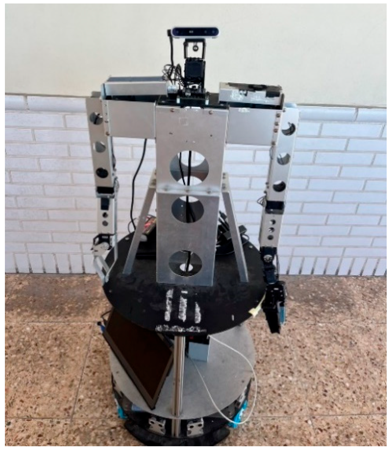
Since the experiment of this study was indoors, we used an omnidirectional wheel mobile robot (WMR). Unlike regular mobile robots, the omnidirectional WMR offers additional movements, such as proper and left-shifting, making it more flexible. This feature enables the omnidirectional WMR to navigate through narrow and intricate indoor spaces easily. The appearance of the omnidirectional WMR we used in this study is shown in Figure 1. The upper part comprises two robotic arms, and the lower part of the depth camera consists of three omnidirectional wheels. The robot’s length, width, and height are 50 cm, 40 cm, and 127 cm, respectively. The head of the robot is an Intel RealSense D415I depth camera (Intel Co., Santa Barbara, CA, USA), which was used to obtain the vision and depth for image recognition and obstacle avoidance. A 2XC430-W250-T servo motor (ROBOTIS Co., Seoul, Republic of Korea) was used to make the robot’s camera rotate freely like a human head.
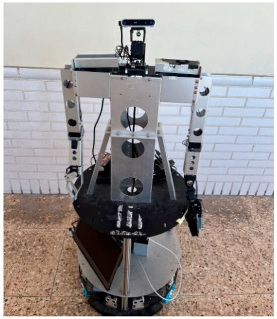
Figure 1.
The outlook of the omnidirectional WMR.
The 2XC430-W250-T motor can control two axes through a single module, which is applied to the neck of the omnidirectional WMR for the pitch and yaw of the rotating head. The robot’s right arm consists of two RX-64 motors (ROBOTIS Co., Seoul, Republic of Korea) for the shoulder, one RX-64 motor for the elbow, and one RX-28 motor for the paw. We changed the robot’s left arm to achieve the grasping function. Under the original right arm design, the wrist was altered to include two MX-28 wrist motors (ROBOTIS Co., Seoul, Republic of Korea) and one claw XM430-W350 motor (ROBOTIS Co., Seoul, Republic of Korea). The above motor communicates with the embedded system through U2D2. The control commands are all calculated on the embedded system NVIDIA Jetson AGX Xavier (NVIDIA Co., Santa Clara, CA, USA). In terms of wheels, the omnidirectional wheel chassis (Innovation First, Inc., Hong Kong, China) has a radius of 240 mm. Three 12V-DC motors placed at 120° and mounted with three omnidirectional wheels provide a rated torque of 68.6 mNm. The omnidirectional electronic module with three motor encoders is mounted on the upper level. Three batteries power the omnidirectional wireless MR; one is a 12V-7Ah lead-acid battery for the robotic arm and neck, the other is an 11V-5800mAh lithium battery for the embedded system, and another is for the wheels 12V-7Ah lead-acid battery.
A depth camera was used in the experiment to achieve object detection and obstacle avoidance. This study used the Intel RealSense LiDAR camera D415I [14]. The camera has an RGB image camera and a LiDAR sensor for depth data. Our previous work used a laptop to program and control the omnidirectional WMR. However, due to the large size and weight of the computer, it was replaced with an embedded system in this study. The embedded system utilized in this study is the NVIDIA Jetson AGX Xavier [15]. The NVIDIA Jetson AGX Xavier is compact, measuring only 105 mm × 105 mm × 65 mm and weighing 280 g. It boasts ten times the energy efficiency and over twenty times the performance compared to its predecessor, the NVIDIA Jetson TX2. The detailed hardware characteristics of the proposed WMR are shown in Table 1.

Table 1.
Hardware characteristics of the proposed WMR.
3. Point Cloud and Image Recognition
In this section, we mainly introduce the methods of point cloud transformation and image recognition. The first part presents the depth map, the pinhole camera model, the relationship of each coordinate system, and the point cloud. Later, the YOLO algorithm, the selected model, and the reasons are introduced.
3.1. Point Cloud Transformation
To construct a 3D point cloud map, we needed to know how to calculate the point cloud in the real-world coordinate system. Firstly, the depth map obtained using the depth camera was required. Secondly, the pinhole camera model converted the depth map into a point cloud. Lastly, the composition of these point clouds formed the 3D point cloud map [16]. In computer vision, a depth map is an image or image channel that contains information about the distance of objects in the scene from a viewpoint. Using a depth camera, we obtained the distance between the camera and the objects for each pixel, as depicted in Figure 2. The depth map was utilized to calculate the point cloud, enabling the measurement of the distance between an omnidirectional WMR (Wheeled Mobile Robot) and detected objects while also helping to navigate around obstacles on the pathway.
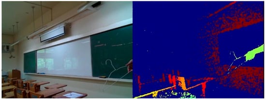
Figure 2.
Image of RGB frame and depth frame.
Figure 3 [17] shows the imaging in the camera during the coordinate transformation process. We need to discuss the relationship between the real-world coordinate system and the camera coordinate system. If the origin of the real-world coordinate system is defined as the camera’s focal point, then the real-world coordinate system is equal to the camera’s coordinate system. During the experiment, since the camera on the omnidirectional WMR moved around, and the origin of the camera coordinate system changed constantly, it was almost impossible for the origin of the real-world coordinate system to be the camera’s focal point. For this purpose, we used the external parameter matrix, composed of a rotation matrix and a translation matrix, a 3 × 4 matrix, as shown in Equation (1) [16].
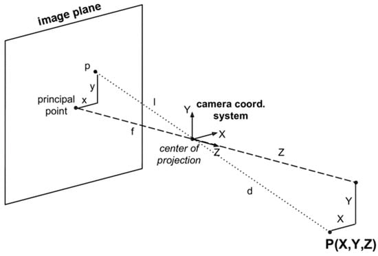
Figure 3.
Camera coordinates.
The depth camera uses the built-in IR projector to project an encoded texture or pattern into the scene. This texture creates a pattern of textured stripes on the object’s surface. The camera sees these texture patterns and uses their deformation to calculate the depth at different points on the object’s surface. By analyzing changes in light patterns, the camera can reconstruct a 3D depth image of the object. The depth camera can calculate the distance from the observed object and output its value. The provided output value will be directly used in subsequent operations.
The point cloud consists of numerous points in 3D space, each with its own set of Cartesian coordinates (X, Y, Z). We can use depth information to perform the reverse conversion. However, we encountered a problem when dealing with the extrinsic parameter matrix, which is a 3 × 4 matrix and cannot be directly inverted. To overcome this problem, we expanded the extrinsic parameter matrix into a square matrix. We added 1/s (disparity) to the left side to satisfy the equation, as shown in Equation (2). These 4 × 4 matrices are referred to as full-rank intrinsic/extrinsic matrices.
We can verify the above equation with the simplest case: the origin of the camera’s coordinate system and the origin of the actual coordinate system are aligned. This means that the rotation matrix and the translation matrix can be neglected and that the image sensor is centered. The inverse of the camera matrix is shown in Equation (3).
According to Equation (2), we can obtain and . Because is depth , the above equation can be expressed as and . This proves that Equation (3) is correct and practicable [16].
3.2. Image Recognition
To let the omnidirectional WMR know where it will go or where it is, we utilize the image recognition algorithm combined with a 3D point cloud map. By identifying some objects we chose, the omnidirectional WMR can obtain the object’s coordinates and plan the path to execute the task. The algorithm of object detection we selected is YOLOv5s. The object detection algorithm with Convolutional Neural Networks can be roughly divided into two genres: the two-stage, represented by Region-CNN (R-CNN), and the one-stage, represented by YOLO. The principle of R-CNN utilizes Selective Search to extract about 2000 region proposals, and then each region proposal is predicted through a CNN channel. The theory of YOLO uses the whole image as input, and then the CNN channel performs the prediction output. Therefore, YOLO has faster speed and lower accuracy than R-CNN. In our experiment, the omnidirectional WMR needed a real-time reaction, so we chose YOLO for object detection. We used the YOLOv5s architecture in the investigation. This architecture was adjusted based on YOLOv5. Next, we will briefly introduce YOLOv5 and YOLOv5s and the reasons for using this architecture.
The architecture of YOLOv5 [18,19] can be divided into four main components: Backbone network, Neck network, Head network, and output layer.
- Backbone network: YOLOv5 uses CSPDarknet53 as its default Backbone network. CSPDarknet53 is a deep convolutional neural network composed of CSP (Cross-Stage Partial) connections.
- Neck network: YOLOv5’s Neck network is used to fuse feature maps of different scales to improve target detection accuracy. YOLOv5 uses the PANet (Path Aggregation Network) structure, which consists of multiple feature pyramid networks (FPNs). PANet can fuse feature information at different levels, enabling the network to perceive targets of different scales better.
- Head network: The Head network of YOLOv5 generates the prediction frame and category probability of target detection. The Head network of YOLOv5 contains a series of convolutional layers and activation functions for extracting features and predicting the location and category of bounding boxes.
- Output layer: The output layer of YOLOv5 is the network’s last layer, which generates the final object detection results. The output layer converts the detected objects into coordinates and category probabilities of bounding boxes and eliminates redundant bounding boxes through non-maximum suppression (NMS).
YOLOv5s and YOLOv5 are different versions of the YOLO series of target detection algorithms, with some differences in network architecture. The following are the main differences between YOLOv5s and YOLOv5.
- Model size: YOLOv5s is the lightest version in the YOLOv5 series, while YOLOv5 is a relatively more extensive and complex version. YOLOv5s is relatively small and suitable for resource-constrained environments, while YOLOv5 is more suitable for running in environments with more computing power.
- Feature fusion network: YOLOv5s and YOLOv5 use different feature fusion networks. YOLOv5s uses PANet (Path Aggregation Network), which consists of multiple feature pyramid networks (FPN). YOLOv5 uses a more complex feature fusion network called SAM (Spatial Attention Module).
- Model depth: YOLOv5s is shallower than YOLOv5. YOLOv5s has fewer layers and fewer parameters, making it have higher speed with limited computing resources, but may sacrifice certain detection accuracy.
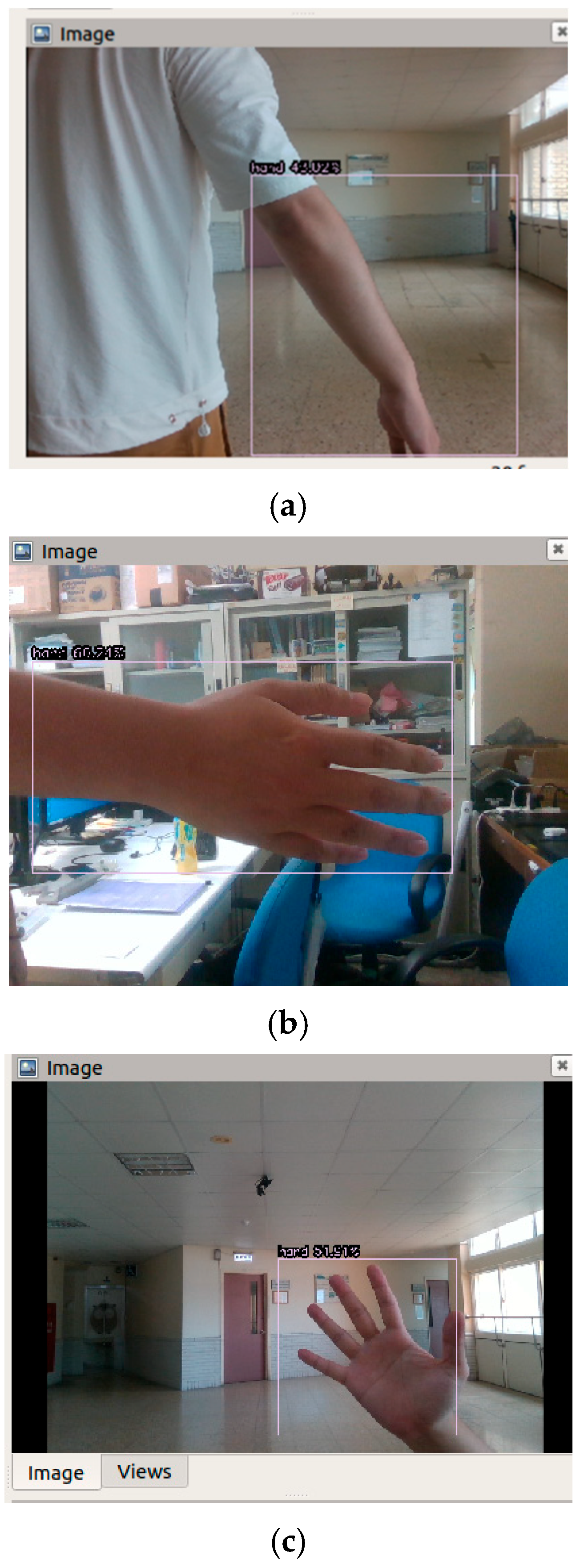
Overall, YOLOv5s is a relatively lightweight version of the YOLOv5 series with a smaller model size and fewer layers, and this meets the requirements of short training time and low precision required by our experiment. Figure 4 shows the results of hand detection. Figure 5 shows the result of doorplate detection.
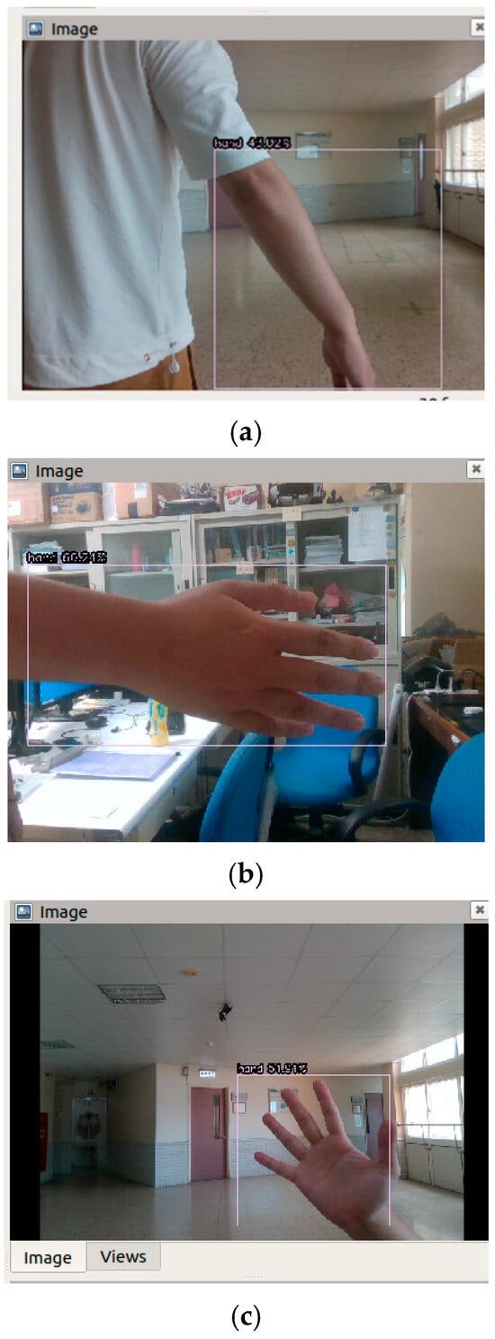
Figure 4.
Results of hand detection for different hand postures and lighting conditions: (a) confidence 48% in condition-1; (b) confidence 60% in condition-2; (c) confidence 51% in condition-3.


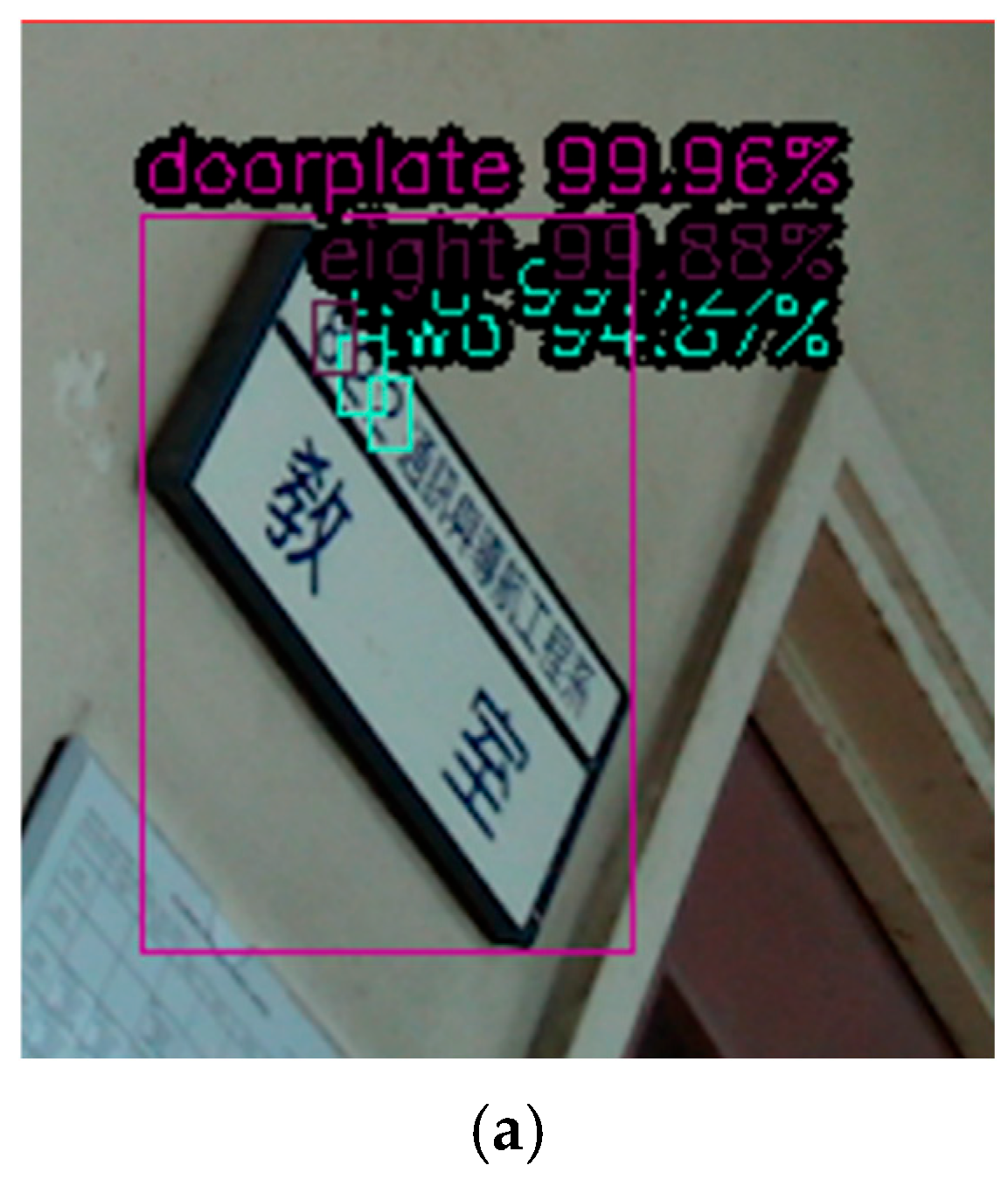
Figure 5.
Result of doorplate detection: (a) doorplate-1 confidence 99% with confidence for first digit-8 99%, second digit-2 99%, third digit-2 94%; (b) doorplate-2 confidence 99% with confidence for first digit-8 99%, second digit-2 99%, third digit-1 89%; (c) doorplate-3 confidence 99% with confidence for first digit-8 99%, second digit-2 99%, third digit-3 99%.
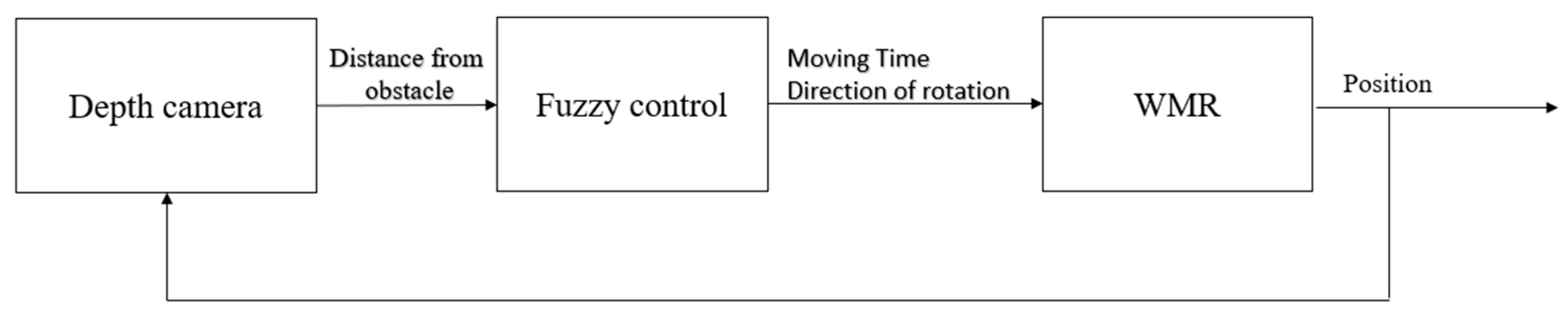
4. Control Scheme
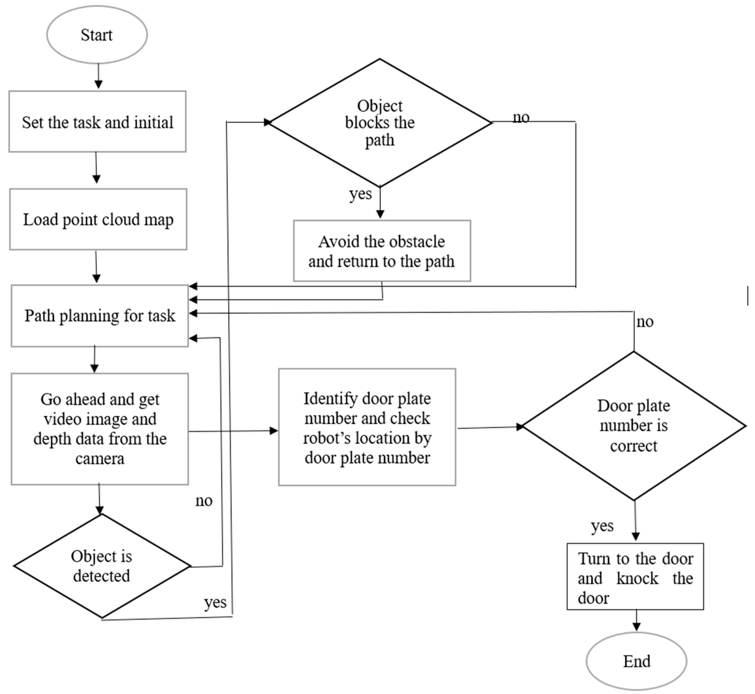
In this experiment, we used the depth data obtained using the depth camera, then corrected and improved the accuracy of the indoor obstacle avoidance and positioning. At the same time, due to the RGB image used for recognition and the experimental environment for pre-collecting data, it was possible to construct a 3D point cloud image and judge the current position of the omnidirectional wheeled robot through object recognition to facilitate the completion of the task. The goal of this experiment was to make the robot first recognize the human hand from the elevator door and use a closed-loop control system to control the mechanical arm to lean forward against the human hand, and then move forward through the pre-planned path using the D3QN algorithm until it reached the destination. For obstacles, we used the Fuzzy theory to avoid the barriers. When an object entered the robot’s judgment frame, the wheels’ speed and steering at the bottom of WMR were adjusted immediately. The closer the distance, the greater the adjustment range of the omnidirectional wheeled robot. When it reached the destination and detected the room number, it started to identify and confirm whether it was the room number of the target classroom. If not, it returned to the original set path to continue the task and then indicated the current position on the point cloud map. The exact process was repeated whenever the YOLOv5 detection system recognized a room number. The depth camera continued judging the distance to walls or obstacles until the correct classroom was identified. The robot stopped in front of the classroom and started using the distance from the depth data to adjust and correct its position. Until the position was correct, the robot knocked on the door as a reminder. Figure 6 shows the flowchart of the robotic arm closed-loop system. In the control law, we formulated the three major coordinate systems in the robot’s vision: the world coordinate system (xw, yw, zw), the camera coordinate system (xc, yc, zc), and the image coordinate system.
- The world coordinate system (xw, yw, zw) is used to coordinate the target object’s position.
- The camera coordinate system (xc, yc, zc) is the camera’s coordinates in the angle.
- The image coordinate system is split into two types of image coordinates: one is image coordinates (x, y), which are continuous image coordinates or space coordinates, with the image’s diagonal as the origin; the other is pixel coordinates (xp, yp), which are discrete image coordinates or pixel coordinates, with the origin at the upper left corner of the image.
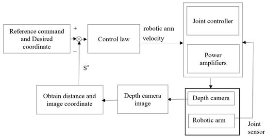
Figure 6.
Flowchart of robotic arm closed-loop control system.
Figure 6.
Flowchart of robotic arm closed-loop control system.

Our control law aims to make the error as small as possible.
It is defined as follows:
where m(t) is the image coordinates and the vector s* represents the expected value.
e(t) = s(m(t)) − s*
The velocity of the robotic arm is vc = (uc, ωc), uc is the speed of the robotic arm, and ωc is the angular velocity of the robotic arm, which can be obtained by (5).
And through the Jacobian matrix (6), the relationship between robotic arm speed and time can be given as (7), where vc is the input:
In the closed-loop control, we defined the following:
- The robotic arm coordinate system is c.
- The desired robotic arm coordinate system is c*.
- The coordinate of the observed objects is the origin “o”
- The vector of “o” for each coordinate system is R.
In the following input, we obtain the camera position and the desired camera position rotation matrix, s = (c*t, θu).
In the robotic arm position rotation matrix, s = (c*t, θu). t describes the translation vector and θu describes rotation, so s* = 0, e = s. According to the above parameters, we can obtain (8).
It can be obtained that the final space velocity vc is (9).
Figure 7 shows a flowchart of the control sequence. Figure 8 shows the experimental environment. Figure 9 shows the path of the task. The Robot Operating System (ROS) [20] is an architecture for computer operating systems specifically designed for robotic software development. It is an open source robotics middleware suite facilitating shared functions, data transfer, application management, and more. In this experiment, the robot carried an embedded system, Intel NVIDIA AGX, which sent instructions to each controller. Through the capabilities of the ROS, the robot can execute tasks synchronously and provide real-time data feedback to each program.
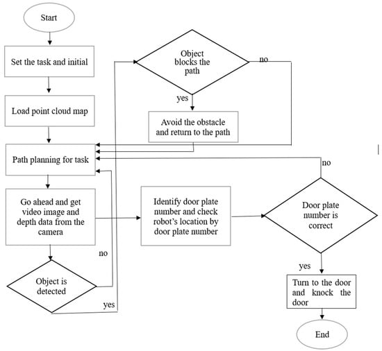
Figure 7.
Flowchart of the control sequence.

Figure 8.
Experimental environment.
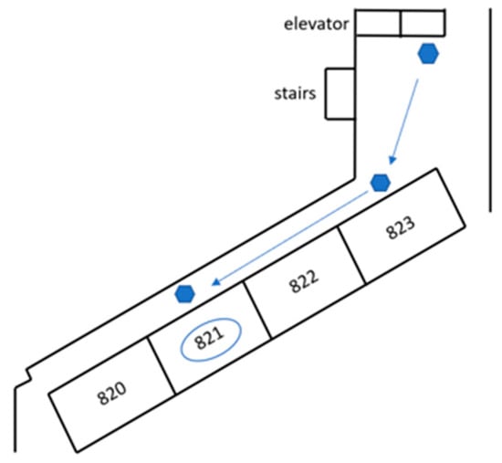
Figure 9.
Path of task and the destination room-821.
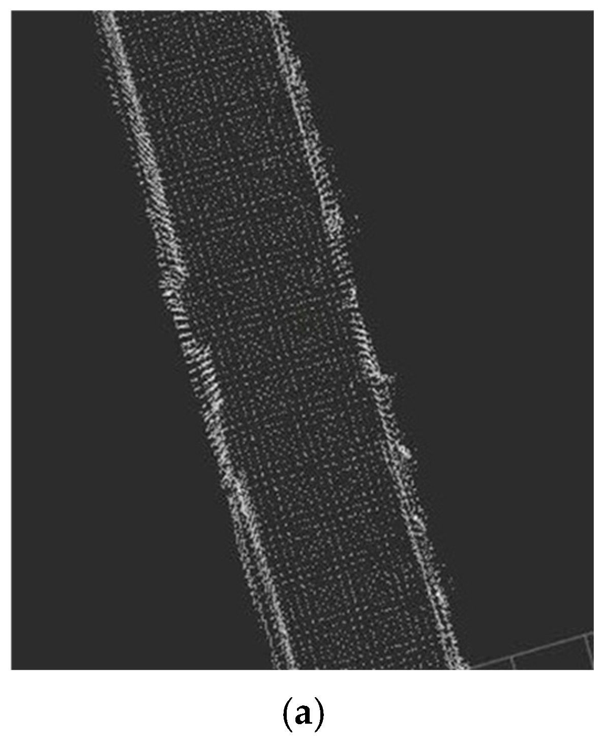
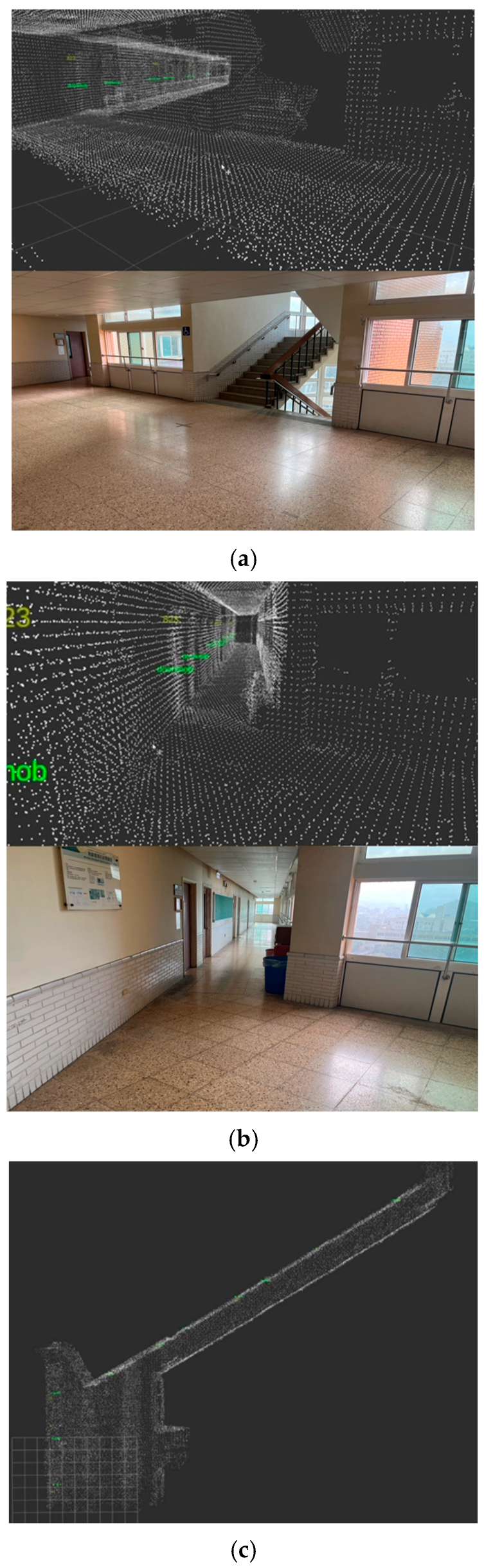
To visualize the 3D point cloud image and easily observe the current position of the omnidirectional WMR along its path, the ROS application RViz is employed as a 3D visualization tool. Figure 10 shows the corridor in the original 3D point cloud map [21].

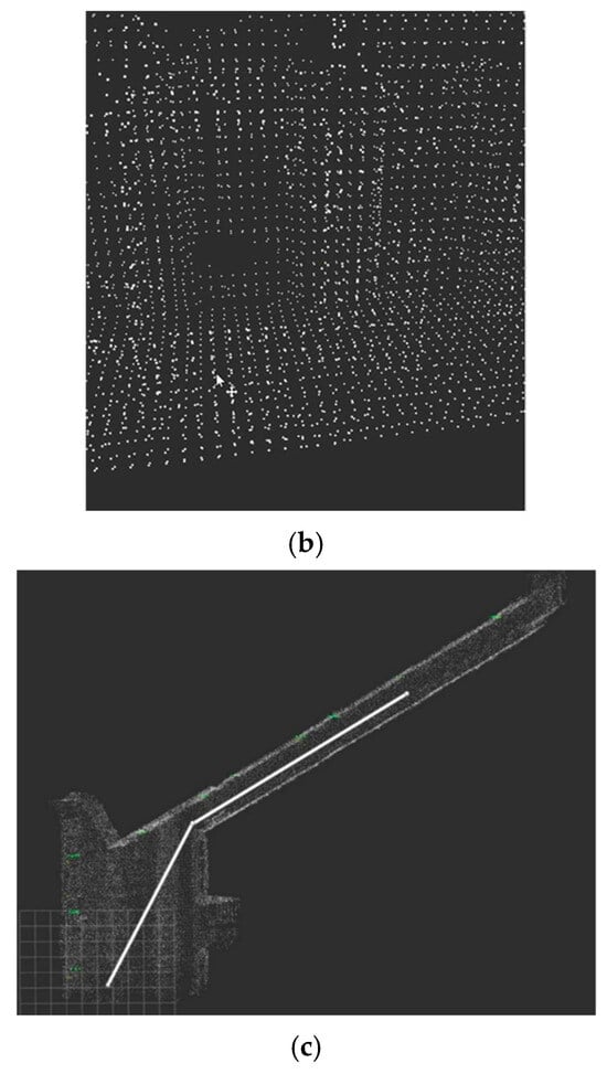
Figure 10.
Corridor in the original 3D point cloud map: (a) top view; (b) side view; (c) combine mission paths and feature objects.
5. Path Planning
In [22], the Markov Decision Process of an underwater glider (UG) was established, the deep reinforcement learning algorithm was utilized for training, and UG’s 3D path planning algorithm was actualized. Here, we only consider 2D path planning. Figure 11 shows the path planning of Q-learning and A* in a dynamic environment [23]. CQL represents the traditional Q-learning, and IQL is its improved Q-learning method. This figure shows that A* cannot successfully reach the end in the dynamic environment. Since our experimental site is also dynamic, we will favor Q-learning rather than traditional path-planning methods. According to the paper ‘Obstacle Avoidance’ proposed by X. Ruan, C. Lin, J. Huang, and Y. Li, a navigation method for robots based on deep reinforcement learning [8], we know that D3QN is better than traditional deep Q-learning, so we chose D3QN as our path planning method.
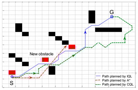
Figure 11.
The path planning of Q-learning and A* in a dynamic environment.
D3QN (Dueling Double Deep Q Network) is a reinforcement learning algorithm combining Q-learning and deep learning. D3QN is an extension and improvement of the traditional Deep Q-Network (DQN) algorithm. DQN is a reinforcement learning algorithm that uses deep neural networks to approximate the Q function. Its basic idea is to build a Q network, take the state as input, and output the Q value of each possible action. Then, the agent chooses the optimal action based on these Q-values to maximize the reward. D3QN extends DQN for more efficient learning and better performance. D3QN uses a distributed architecture where multiple agents interact and share experiences in the environment. These agents are trained on different instances of the environment and then pool their experience together to improve the training of the Q-network. In addition to the distributed architecture, D3QN also introduces two key technical improvements. The illustrations of DQN and D3QN [8] are shown in the Supplementary Materials section.
The double-Q network is used to solve the estimation bias problem in DQN. In DQN, the same network is used to estimate the target Q value and decide to choose the optimal action. This easily leads to an overestimation of the Q value, affecting the stability and performance of learning. D3QN alleviates this problem by using two separate Q-networks, one for estimating the target Q-value and the other for selecting optimal actions. Priority replays are for more efficient use of experience replays. In DQN, the agent stores its experience in a replay cache and then randomly samples from it for training. Priority playback adjusts the sampling probability of samples by giving different priorities according to the importance of experience, and trains the network to be more targeted. This way, experiences contributing more to learning are more likely to be selected for training, improving learning efficiency and performance.
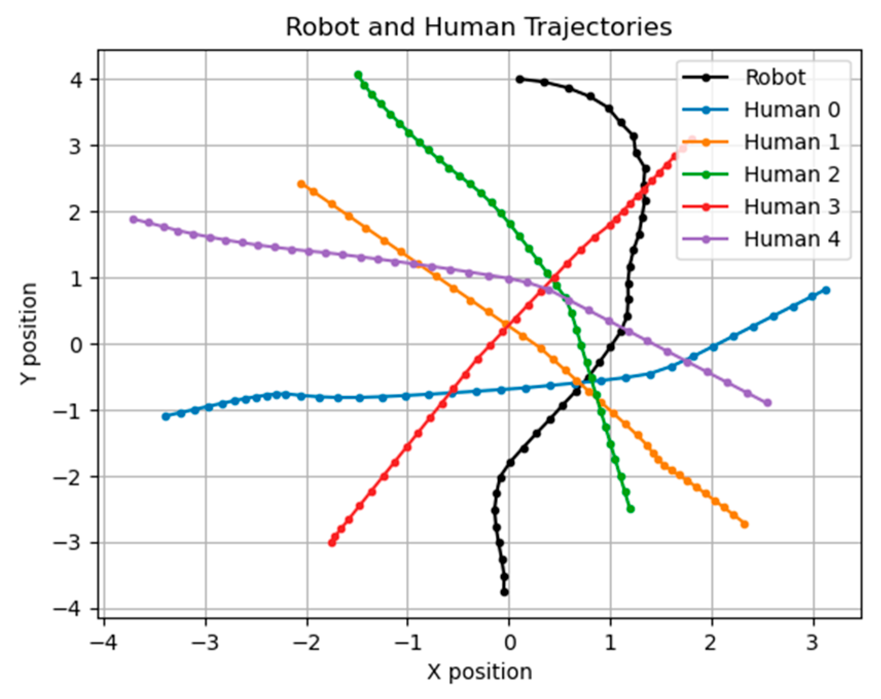
A large part of the experimental results in D3QN will be affected by parameters such as reward values, penalty values, etc., and different parameters will make the results very different, so how to define related parameters becomes very important. Initially, we used the most straightforward trial and error method to find the best solution, but the results were not ideal. Figure 12 shows the trajectories of , , where is the reward for reaching the destination and is without collision. is the penalty for collision, and the total reward is shown in (10). Different parameters’ trajectories are shown in the Supplementary Materials section.
Reward = x1 + x2 + x3
Figure 12.
Trajectories of , ; the unit of the X–Y axis is meters.
Our simulation goal is to let the robot go from coordinates (0, −4) to (0, 4) without collision. Table 2 shows the parameters and time to reach the endpoint.
Table 2.
Different sets of parameters and the time consumed.
Since the parameters cannot be calculated, we use the genetic algorithm to determine various parameters and conduct simulations. We set the fitness function in the genetic algorithm as
,
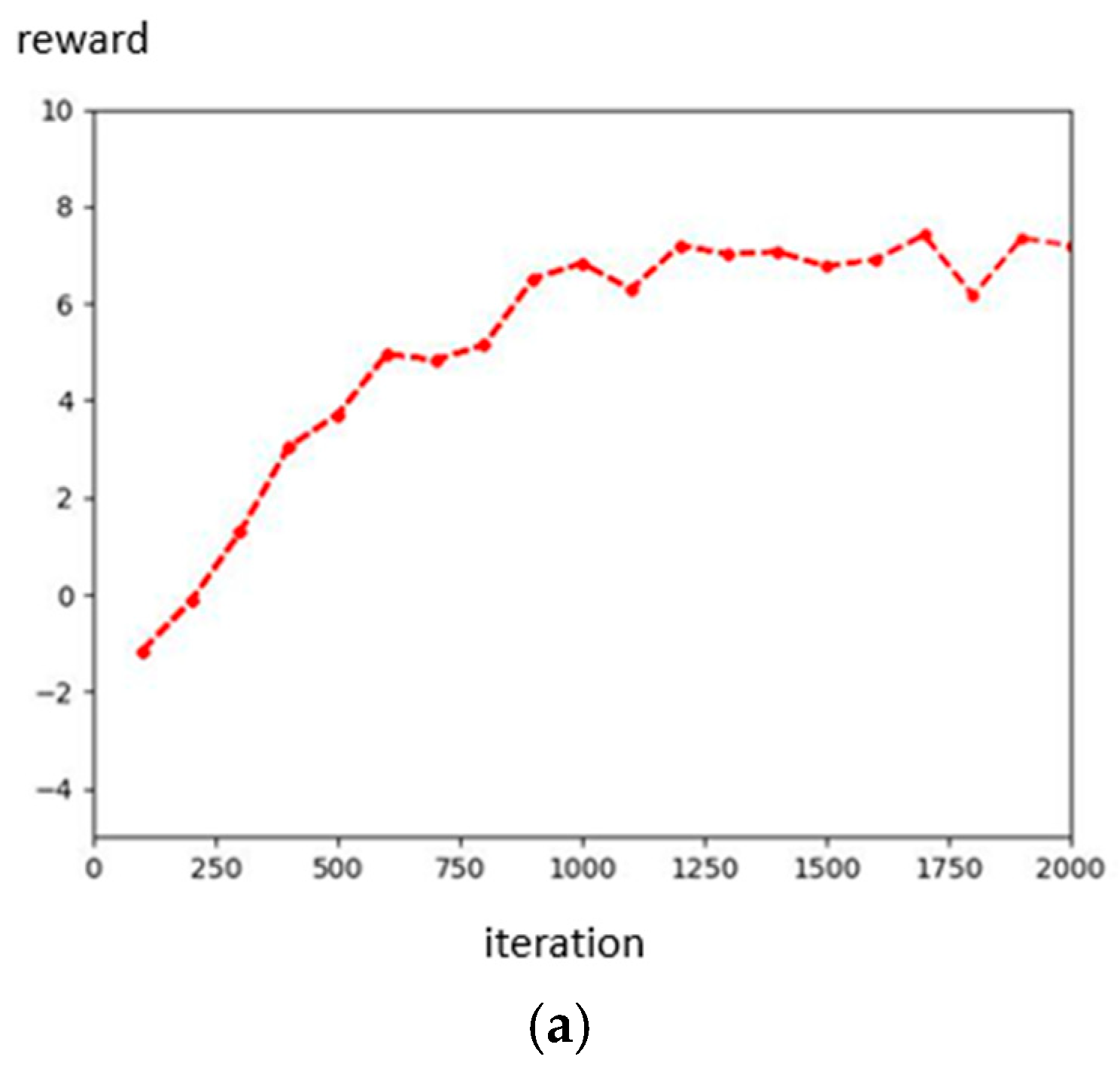
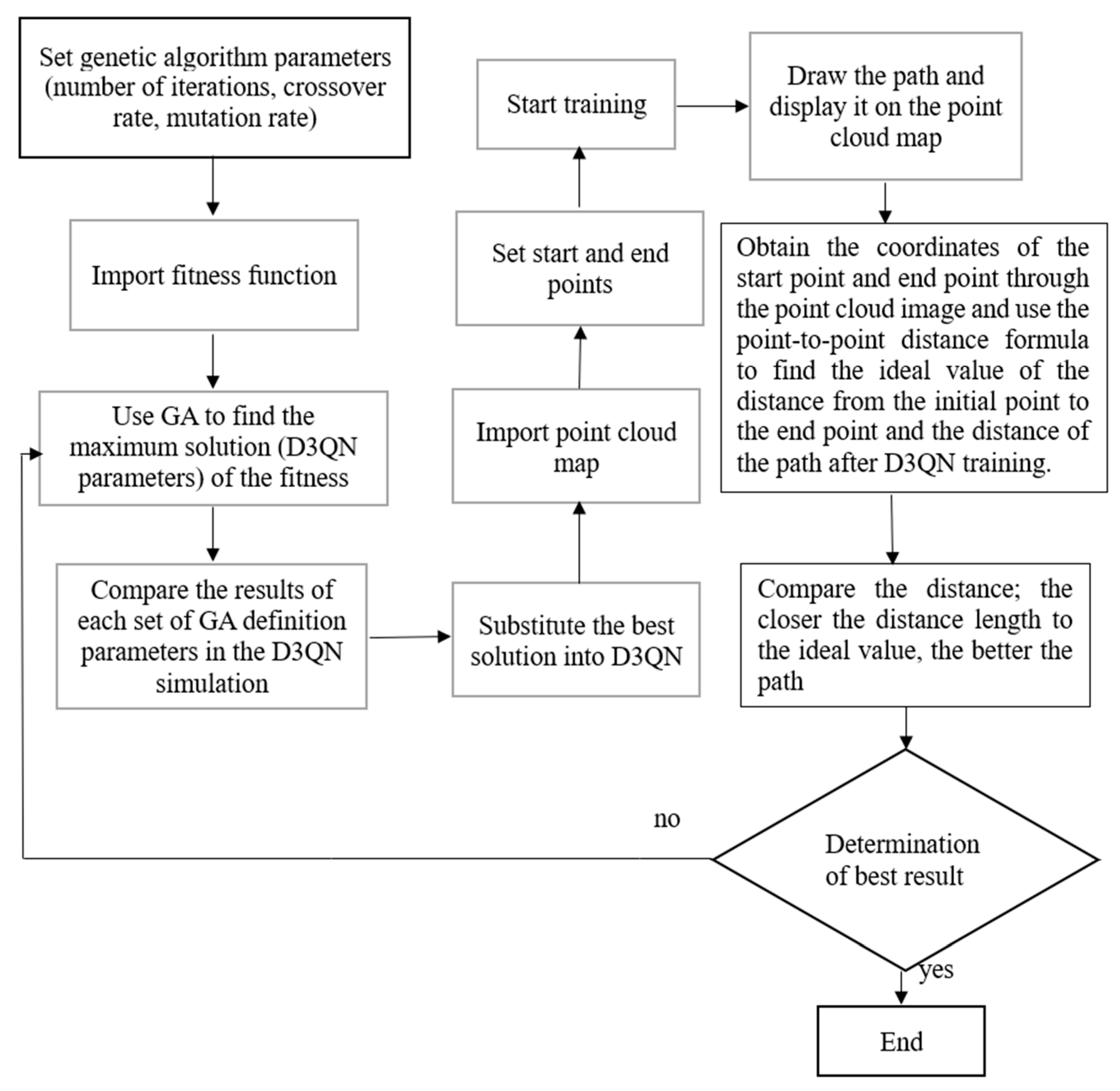
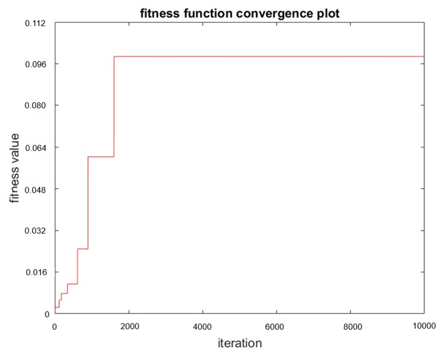
We defined the limit value of and t, because we want our robot to avoid overfitting when converging like in Figure 13. The t is greater than eight because the initial speed in the robot simulation is 1 m/s. Then, we set the initial population to 100, the crossover rate to 0.5, and the mutation rate to 0.01, and used roulette wheel selection to choose the next generation. Then, using the fitness function, we obtain the best value of parameters where , , Then, we designed and compared another set of parameter values that would obtain the same reward. Figure 14 shows the results for the 3rd parameters and rewards. Figure 15 shows the results for the defined parameters and rewards. By comparing Figure 14 and Figure 15, we can find that, even under the same reward value, the trajectories obtained by the experiment will differ due to the other parameter values of the components. Figure 16 shows the architecture of D3QN with GA. Figure 17 shows the fitness of the GA process.

Figure 13.
Over-fitting reward convergence plot.
Figure 14.
The results for the 3rd set of parameters; the unit of the X–Y axis is meters. (a) D3QN reward using the 3rd set of parameters results in the reward. (b) Using the 3rd set of parameters result.

Figure 15.
The result of the GA-defined parameters; the unit of the X–Y axis is meters. (a) Reward of GA-defined parameters result. (b) GA-defined parameters result.

Figure 16.
The architecture of D3QN with GA.
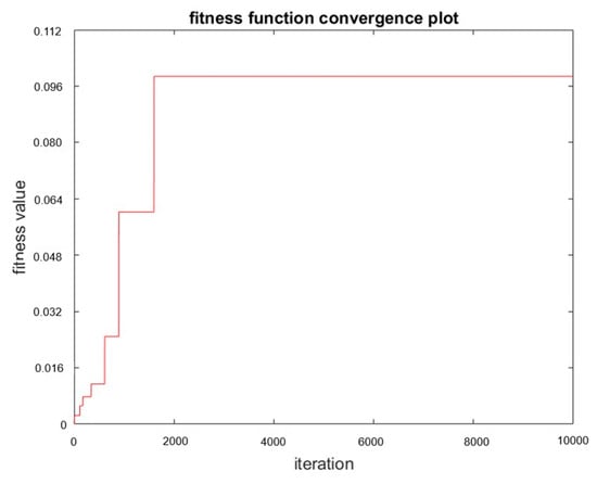
Figure 17.
Fitness of the GA process.
In addition, we also tried to use the evolutionary algorithm to define the parameters. Our objective function is similar to the genetic algorithm’s fitness function and uses the same GA sets. However, the speed is still slower than the parameters obtained using the genetic algorithm, and we obtained the following best values of the parameters: , , and . Figure 18 shows the resulting graph using the evolution algorithm to define the parameters.
Figure 18.
The result of using the evolutionary algorithm to define the parameters; the unit of the X–Y axis is meters.
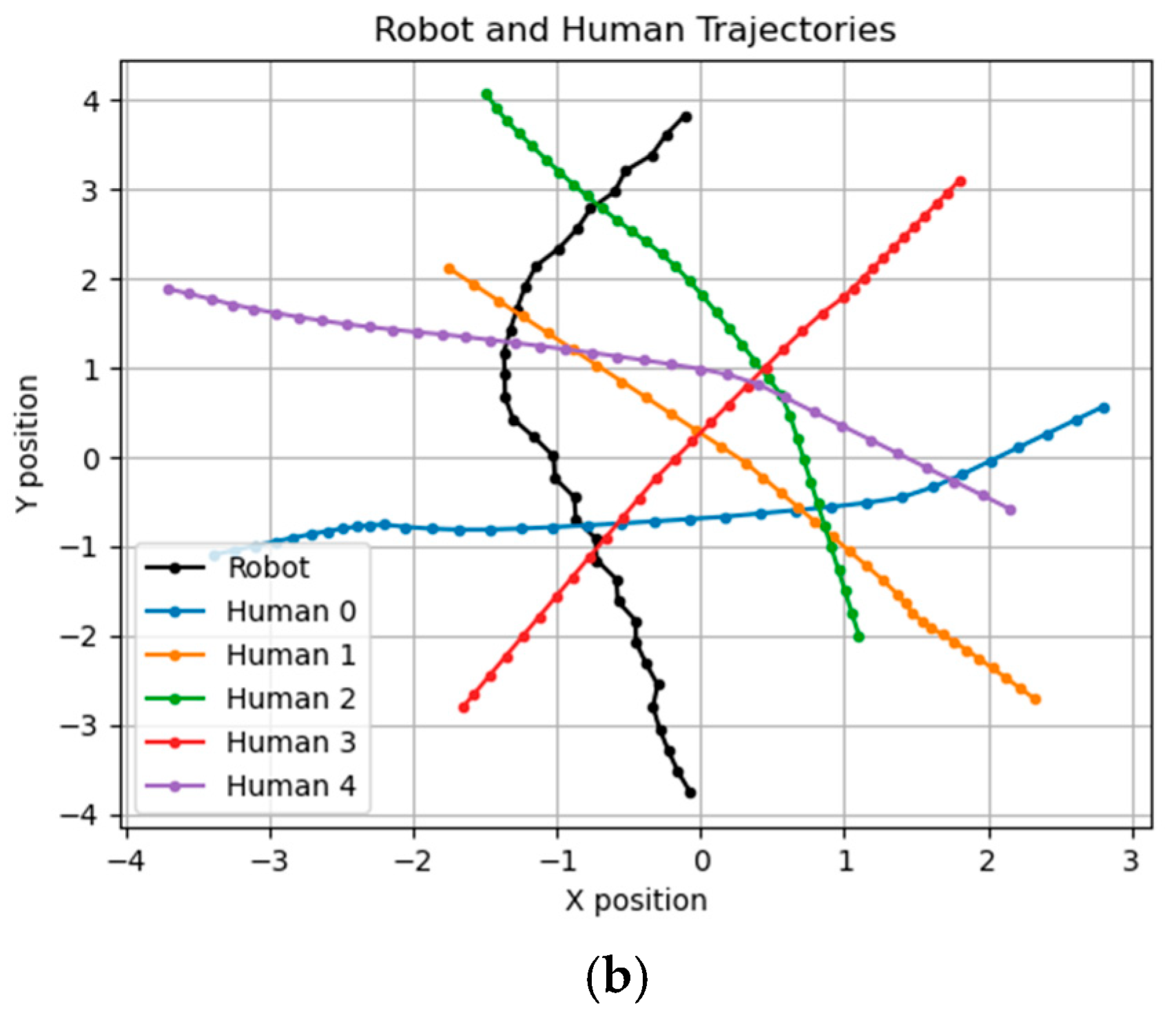
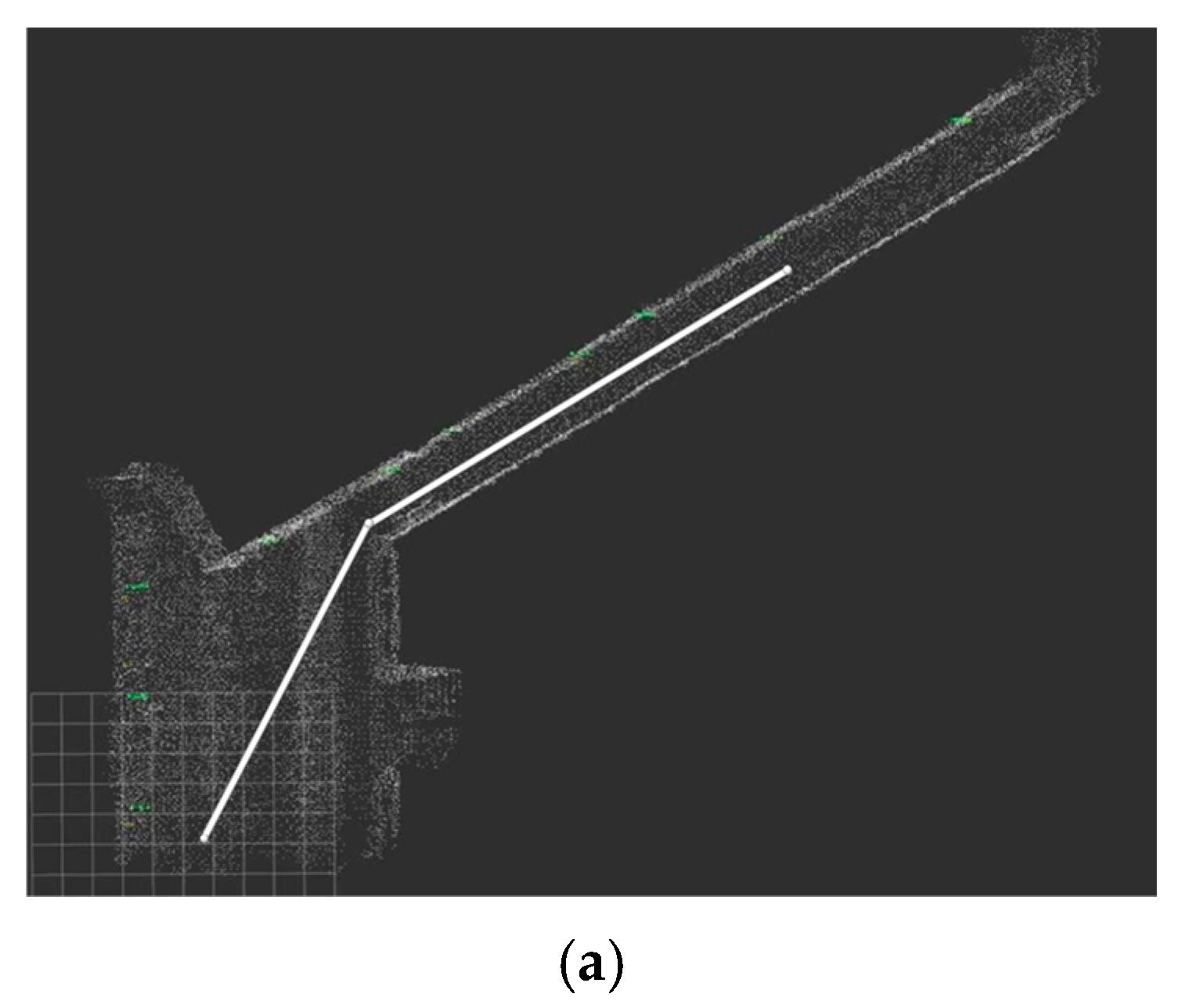
In the end, according to the architecture of D3QN with GA flowchart, Figure 19 shows the ideal and actual paths with optimal parameter values: , , .
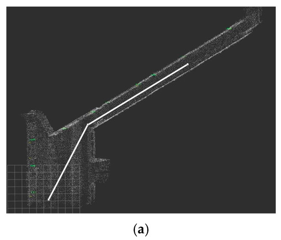
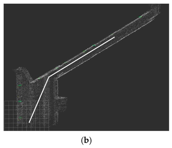
Figure 19.
Ideal path and deployment path: in the actual path, the robot moves closer to the left-side wall instead of closing to the right-side wall in the ideal path. (a) Ideal path. (b) Actual path.
6. Obstacle Avoidance
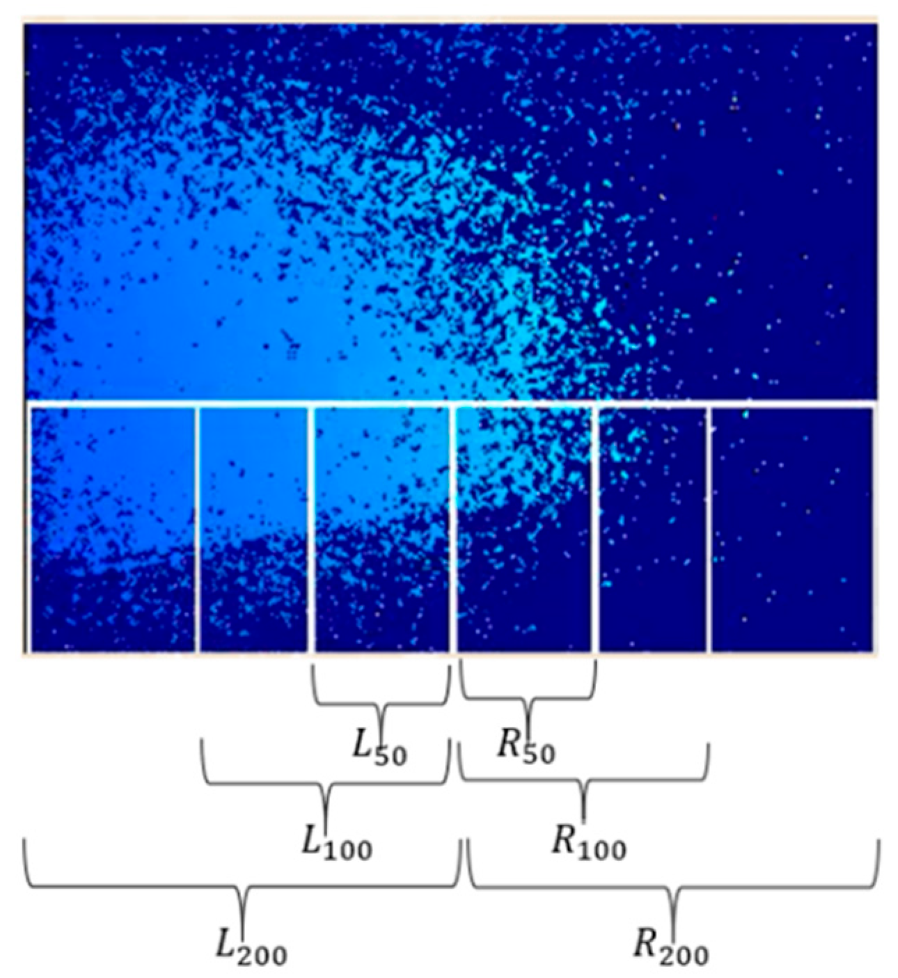
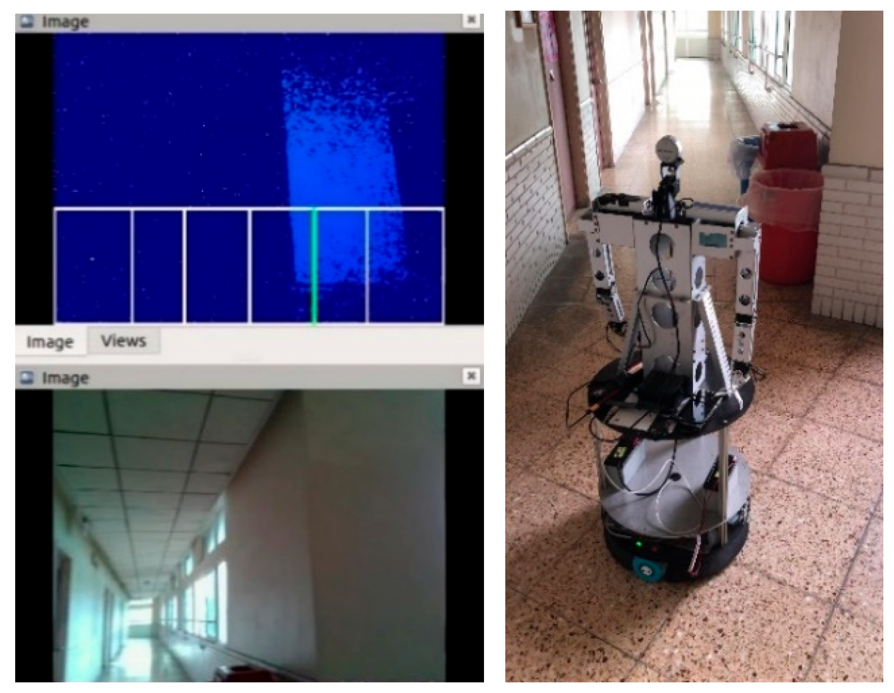
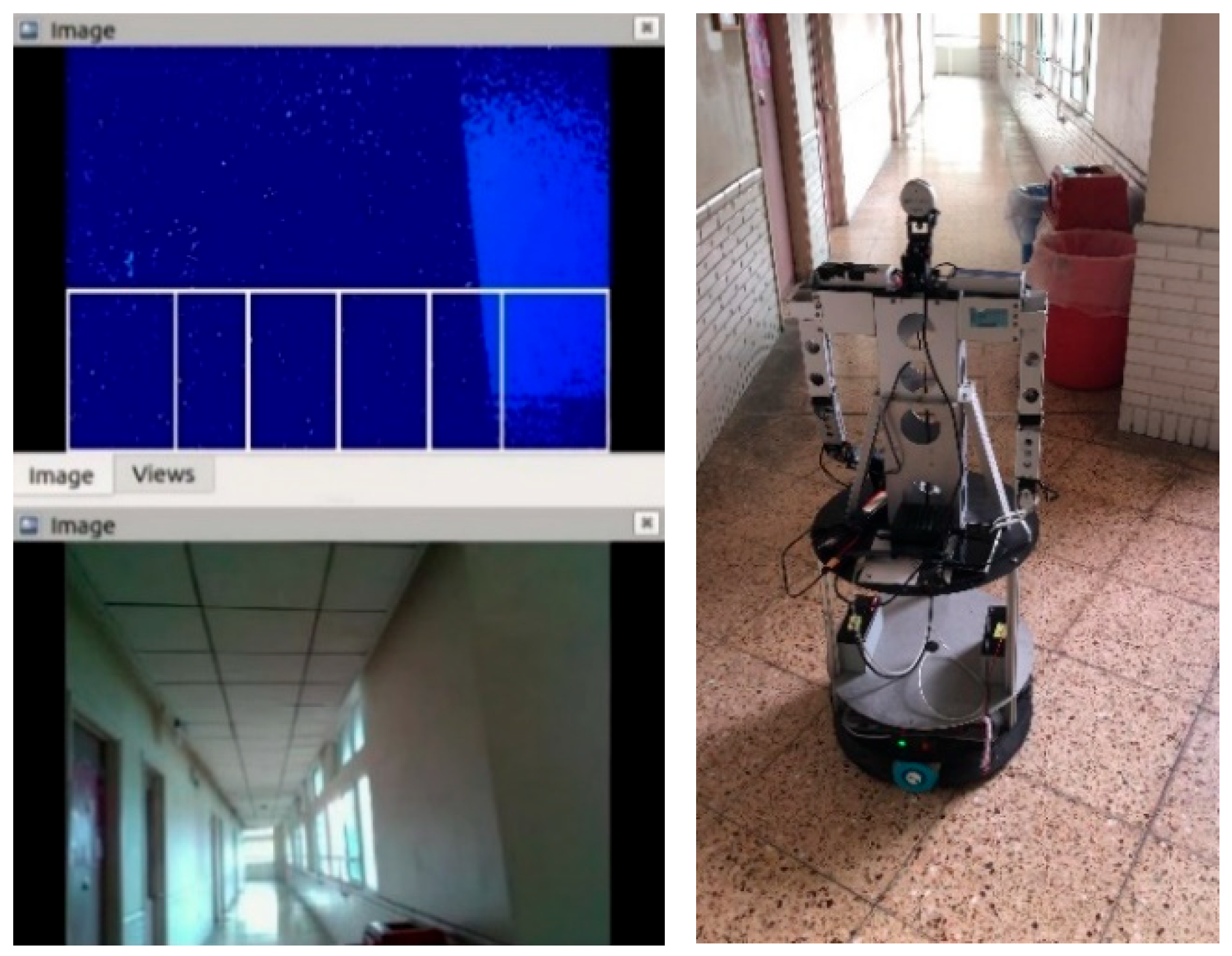
We implemented the following methods to enhance the collision avoidance performance of omni-wheeled robots. First, a depth image was obtained using a wide-angle depth camera. Then, the camera’s frame was segmented into several parts, respectively, as shown in Figure 20, and the depth image was analyzed to determine the location of obstacles or other objects (such as walls) to control WMR. Since the depth distance is determined from the maximum value in the depth image, stationary objects can be detected early. Even when objects appear suddenly (for example, a pedestrian passes by and appears in the picture), the decision-making process can still function effectively. Then, the robot was programed to avoid obstacles according to the fuzzy rules we set.
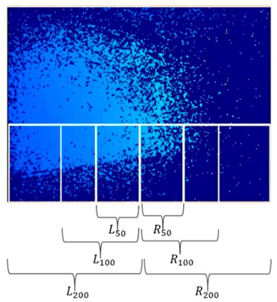
Figure 20.
Parts of the camera’s frame.
L_50: Number of pixels with a depth less than 50 cm in the three boxes on the left side.
R_50: Number of pixels with a depth less than 50 cm in the three boxes on the right side.
L_100: Number of pixels with a depth less than 100 cm in the two boxes on the left side and the closest middle box.
R_100: Number of pixels with a depth less than 100 cm in the two boxes on the right side and the closest middle box.
L_200: Number of pixels with a depth less than 200 cm in the box on the left side and the closest middle box.
R_200: Number of pixels with a depth less than 200 cm in the box on the right side and the closest middle box.
The fuzzy rules are as follows:
R1: if L is near and M is near and R is near then T is LG and P is TR.
R2: if L is near and M is near and R is medium then T is LG and P is TR.
R3: if L is near and M is near and R is far then T is LG and P is TR.
R4: if L is near and M is medium and R is near then T is ST and P is GT.
R5: if L is near and M is medium and R is medium then T is MD and P is TR.
R6: if L is near and M is medium and R is far then T is MD and P is TR.
R7: if L is near and M is far and R is near then T is ST and P is GT.
R8: if L is near and M is far and R is medium then T is ST and P is TR.
R9: if L is near and M is far and R is far then T is ST and P is TR.
R10: if L is medium and M is near and R is near then T is LG and P is TL.
R11: if L is medium and M is near and R is medium then T is LG and P is TR.
R12: if L is medium and M is near and R is far then T is LG and P is TR.
R13: if L is medium and M is medium and R is near then T is MD and P is TL.
R14: if L is medium and M is medium and R is medium then T is ST and P is GT.
R15: if L is medium and M is medium and R is far then T is ST and P is TR.
R16: if L is medium and M is far and R is near then T is ST and P is TL.
R17: if L is medium and M is far and R is medium then T is ST and P is GT.
R18: if L is medium and M is far and R is far then T is ST and P is GT.
R19: if L is far and M is near and R is near then T is LG and P is TL.
R20: if L is far and M is near and R is medium then T is LG and P is TL.
R21: if L is far and M is near and R is far then T is LG and P is TL.
R22: if L is far and M is medium and R is near then T is MD and P is TL.
R23: if L is far and M is medium and R is medium then T is MD and P is TL.
R24: if L is far and M is medium and R is far then T is MD and P is TL.
R25: if L is far and M is far and R is near then T is ST and P is TL.
R26: if L is far and M is far and R is medium then T is ST and P is GT.
R27: if L is far and M is far and R is far then T is ST and P is GT.
Among the detected areas, the left (L), middle (M), and right (R) correspond to L200~L50, L50~R50, and R50~R100, respectively. Each part detects the nearest obstacle and calculates the distance between the obstacle and the robot. These distances of the three obstacles are used as inputs for the fuzzy control system, which has three fuzzy sets: near, middle, and far. The output of the fuzzy control system consists of two variables: time (T) and pixel (P). The output time (T) is used to control the duration of wheel turning, and its fuzzy sets include long (LG), medium (MD), and short (ST). The pixels (P) control the direction of rotation, and their fuzzy sets are as follows: turn right (TR), turn left (TL), and go straight (GT).
The fuzzy control system takes the distances of the three obstacles as input. It calculates the appropriate values for time and pixels to effectively control the robot’s behavior in avoiding obstacles. The membership functions of the fuzzy sets are shown in the Supplementary Materials section. Figure 21 shows the Fuzzy control scheme. Figure 22 shows boxes of obstacle avoidance in the depth map and YOLOv5 detection. In previous works, we used the gradient descent method to obtain the optimal center location and width of the Gaussian fuzzy set. However, a disadvantage of this is that it increases the process cost. In this paper, to reduce the computing time, we only used the traditional fuzzy set in the fuzzy rule.
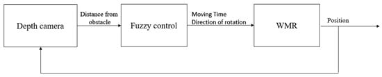
Figure 21.
Fuzzy control scheme.
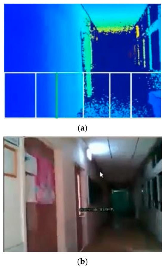
Figure 22.
Boxes of obstacle avoidance in the depth map and YOLOv5 detection. (a) Depth Image. (b) RGB Image with door knob detection confidence 81%.
In Figure 23, the obstacle avoidance rule 6, which is , is satisfied, so the omnidirectional WMR rotated left until there was no satisfied obstacle avoidance rule, as shown in Figure 24.

Figure 23.
The obstacle avoidance rule 6 is satisfied.

Figure 24.
Rotating left until there was no obstacle.
7. Experimental Results
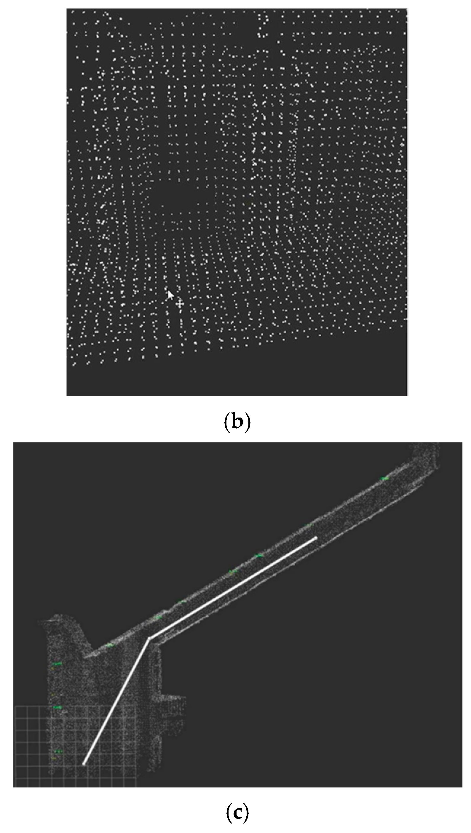
In this study, the robot obtained various data using the depth camera and performed tasks such as navigation, obstacle avoidance, and object detection. The depth distance was obtained using the depth camera to correct the robot’s position during the mission. The robot performed the next step when it recognized the characteristic object. Before experimenting, we needed to prepare some actions to make the experiment go smoothly. The first was to train a set of good weights for YOLOv5 to recognize images, and the second was to measure the experimental space and the length, width, and height, and then convert this information into the coordinates of the 3D point cloud map to allow for the robot to perform indoor navigation and positioning. Figure 25 shows the feature object. Figure 26 shows the experimental 3D point cloud map.
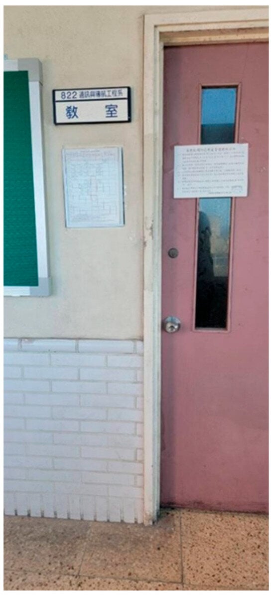
Figure 25.
Feature object.

Figure 26.
The experimental 3D point cloud map: (a) Scene 1; (b) Scene 2; (c) top view of Scene 2.
7.1. Robotic Arm Control
The first thing we need to do before guiding blind people is to use the robotic arm to hold a human hand. Regarding the whole arm’s control system, we will divide it into the following parts to explain.
- Control wheel steering arm:
Set the robot’s initial position and the orientation of its camera by using a point cloud map, then use a depth camera to locate the position of a human hand and execute a program to make the robot approach the ideal position to grasp the human hand.
- 2.
- Obtaining the coordinates of the human hand:
The 3D coordinates of the human hand were obtained using the depth camera. The camera can perform depth sensing through an infrared emitter and an infrared camera to obtain the three-dimensional position of objects in the scene. In this experiment, the robot sensed the position of the human hand using the camera and obtained the 3D coordinates of the human hand.
- 3.
- Calculation of the relative relationship between the robot hand and the human hand:
After obtaining the coordinates of the human hand, it is necessary to calculate the relative relationship between the robot arm and the human hand. We obtained the relative angles of each joint relative to the target position using the D-H model and used them to control the movement of the robot hand.
- 4.
- Controlling the robot hand to hold the human hand:
In the experiment, due to the high precision of the arm motor, we simplified the control system to be directly controlled by the host NVIDIA Jetson Xavier.
- 5.
- Closed-loop control of wheels and robotic arm:
During the holding process, due to various factors that may cause slight changes in the positions of the human and robotic hands, closed-loop control was required to maintain stability. Closed-loop control uses the depth camera to continuously monitor the human and robotic hands’ positions and adjust the robotic hand’s movement based on the difference to maintain a stable grip.
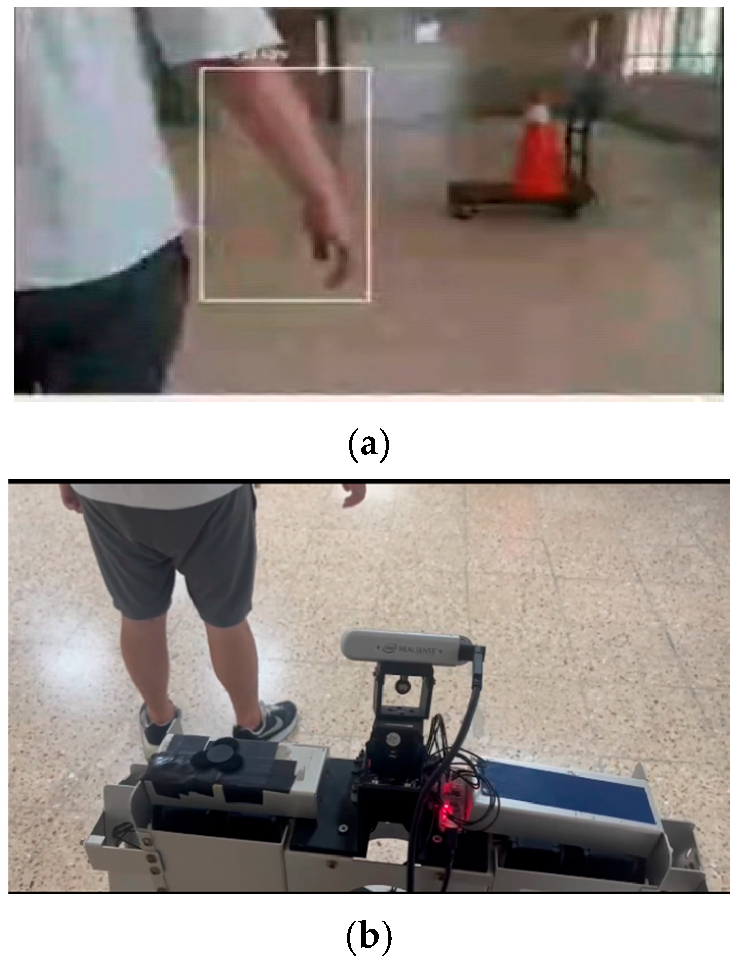
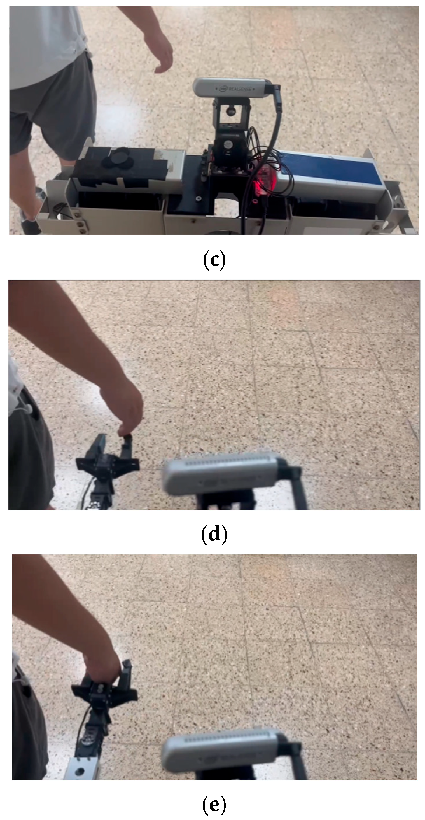
Figure 27 shows the process of robotic arm control. The moving distance error of the robot from the depth camera is less than 2% in 100 cm depth, which is less than 2 cm. Since the claw of the robot can open 10 cm, the robot can grasp the blind person without a problem.


Figure 27.
The process of robotic arm control: (a) robot detects a human hand; (b) robot shifts right; (c) robot moves to the human hand; (d) robot raises its left arm; (e) holding the blind person’s hand.
7.2. Going to the Designated Place
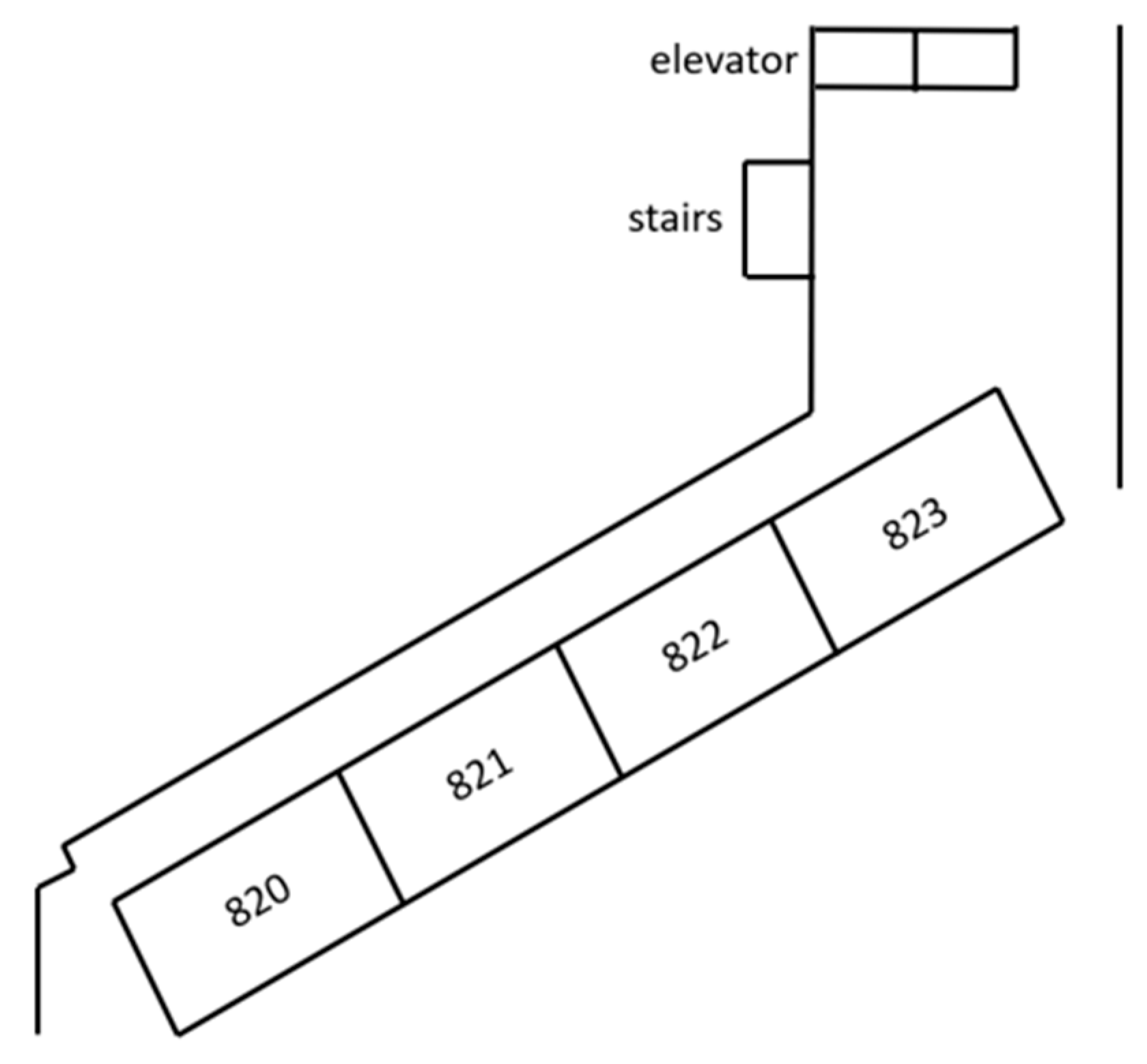
The starting point of the experiment was set 1 m in front of the elevator, and the robot was placed at the initial position, as shown in Figure 28. For the robot to reach the destination smoothly, the robot must obtain real-time images from the depth camera, detect the door from the picture, guide the robot closer to the corridor, and gradually approach the destination. In this experiment, the destination was Room 821.
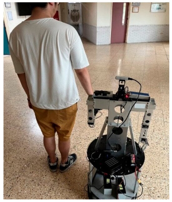
Figure 28.
Starting position.
When the robot was close enough to the door, the robot started to turn right. The robot then entered the hallway. At the same time, the robot began searching for the next predetermined point, which was the trash can. When the trash can was detected, the robot stopped spinning and walked across the hallway. Figure 29 shows the turning spot and the trash can’s location.
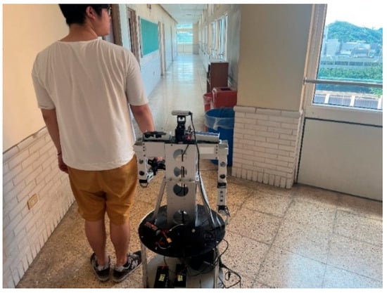
Figure 29.
Turning spot and the trash can’s location.
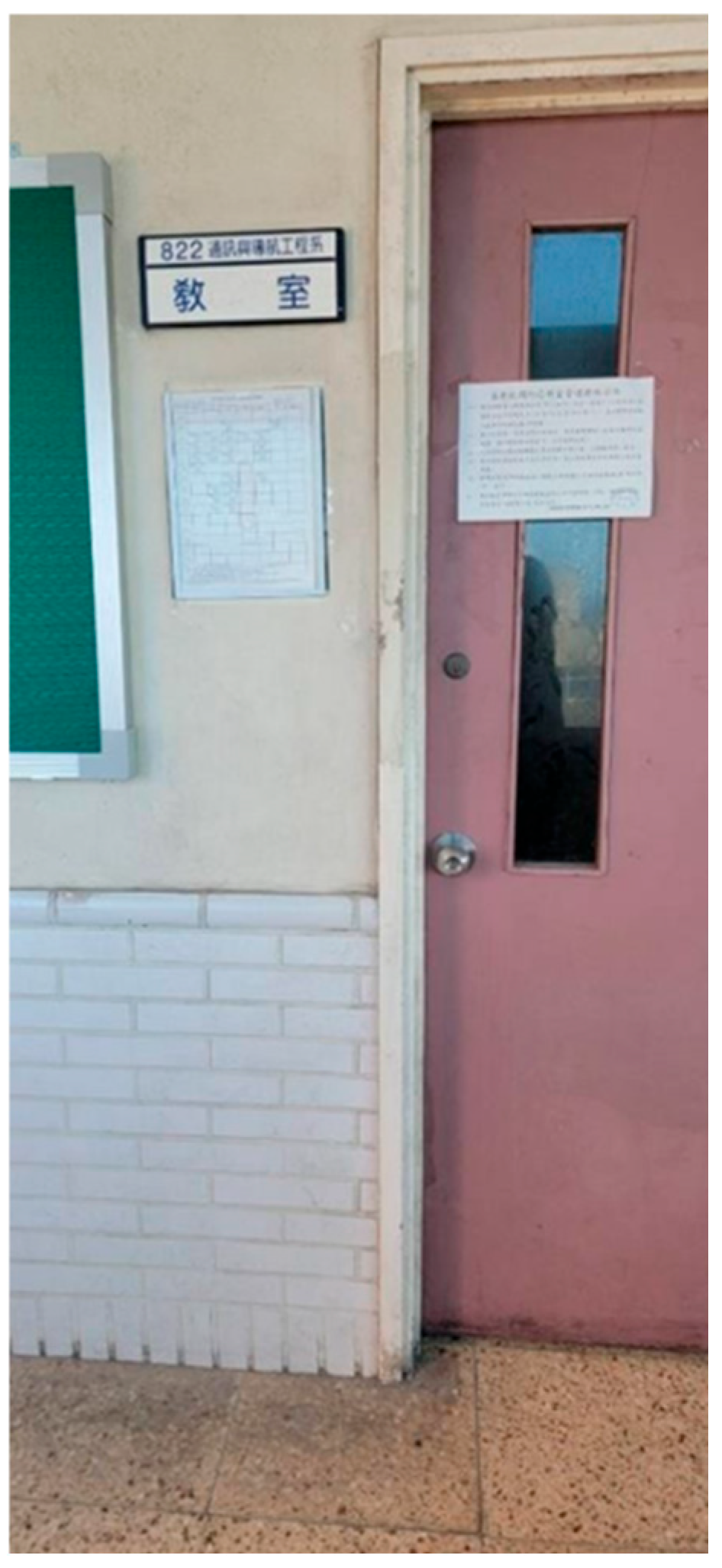
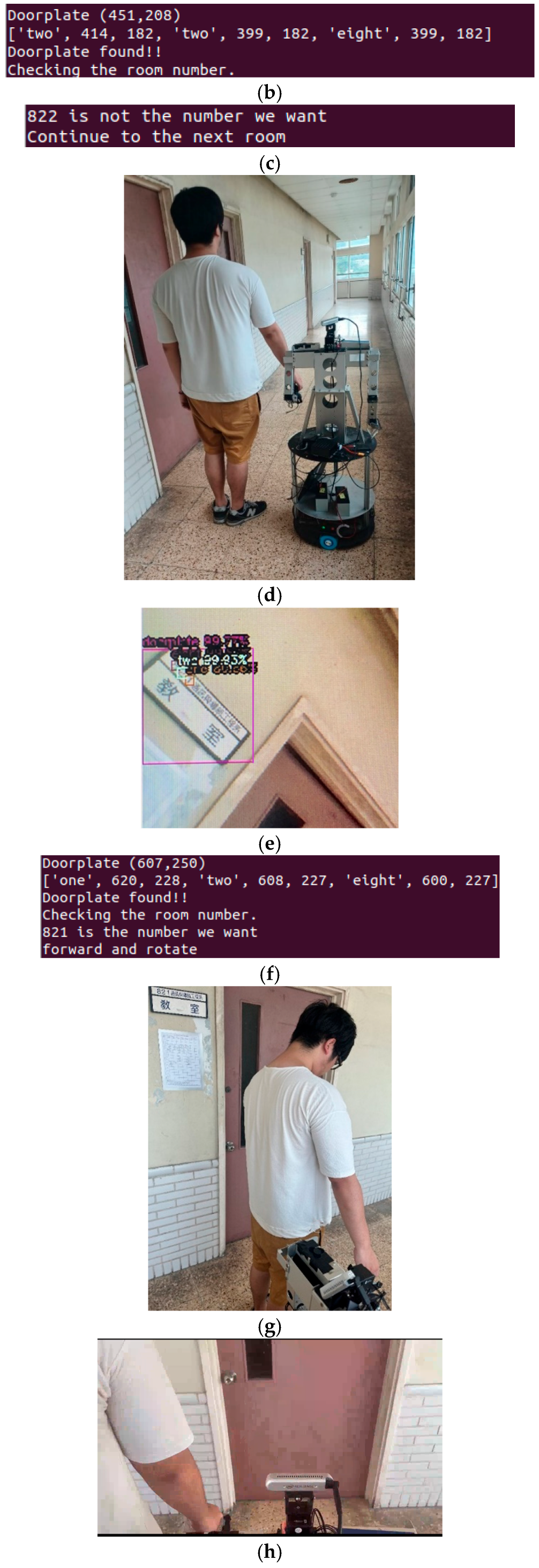
When the robot passed through the hallway, the robot used the depth camera on its head to detect the room number on the side wall, as shown in Figure 30. If a room number was seen, the robot stopped to check the number, and if the room number was wrong, the robot moved onto the next room. Take classroom 821, the experimental destination, as an example. When room 822 was detected, the system displayed the wrong door number, and then the robot continued to move until it found the correct door number, as shown in Figure 31. Then, the robot turned to face the 821 classroom door. Since all the pattern recognition rates of the room numbers are greater than 90%, we set the threshold of the image detection accuracy to 0.9. During the experiment, all room numbers could be successfully identified. According to the preset room number, the robot can be controlled to search for the desired room.
Figure 30.
Detecting the room number on the side wall.
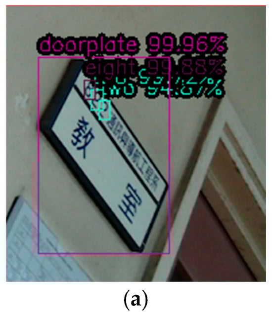

Figure 31.
Find the correct house number: (a) Room 822 is detected; (b) checking the number; (c) Room 822 is not the desired room; (d) the robot continues to move; (e) Room number 821 is detected; (f) desired room found; (g) arriving in classroom 821; (h) turning to face the 821 classroom door.
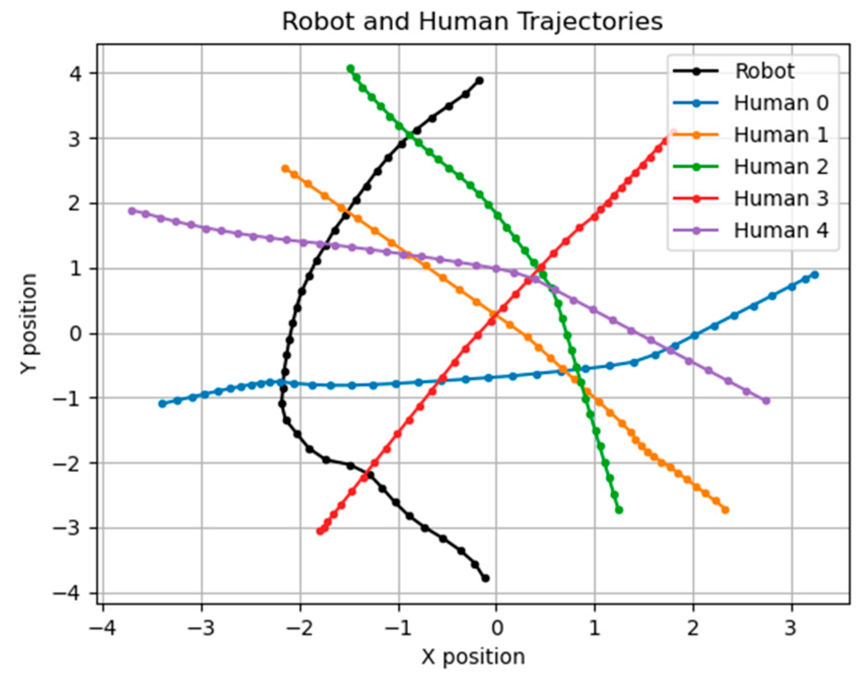
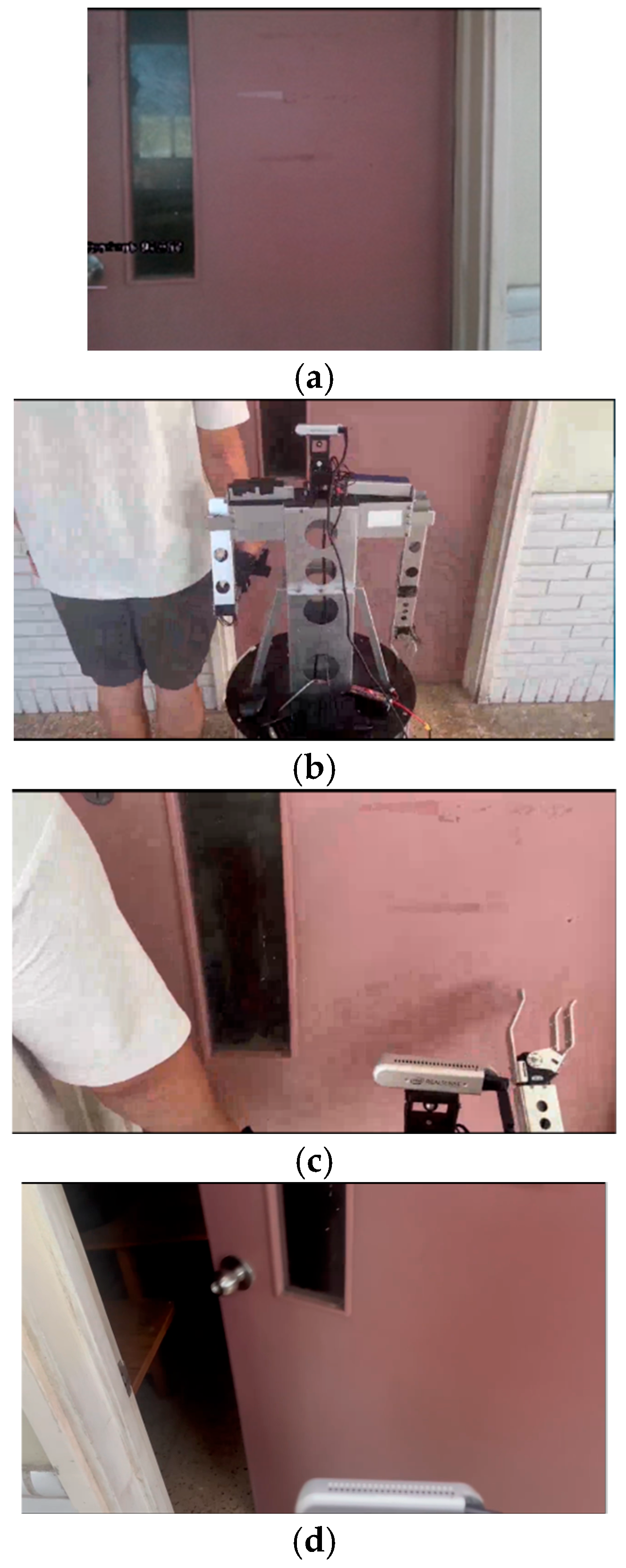
After facing the door, the robot used a depth camera to obtain the coordinates of the doorknob. The doorknob’s coordinates were used to calculate the distance between the robot and the doorknob. Then, the robot started moving to the classroom door and knocking. Figure 32 shows the process of knocking on the door. Figure 33 shows the trajectory of the robot on the point cloud map.

Figure 32.
The process of knocking on the door: (a) the robot detects the doorknob; (b) robot forwards to the door; (c) robot knocks at the door; (d) the human opens the door.
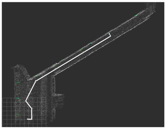
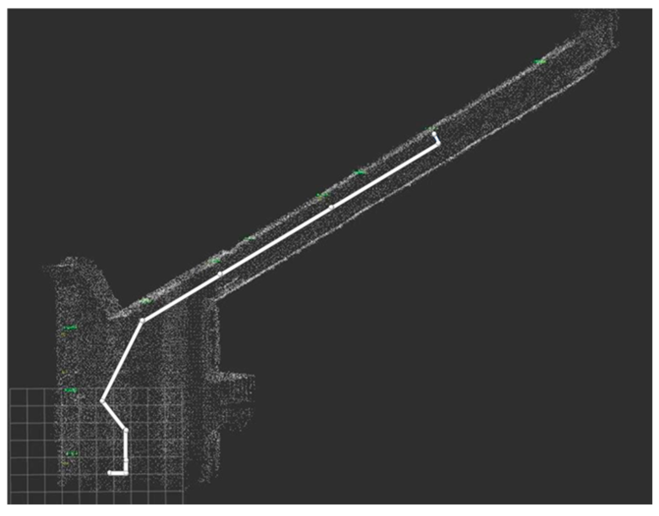
Figure 33.
The trajectory of the robot on the point cloud map.
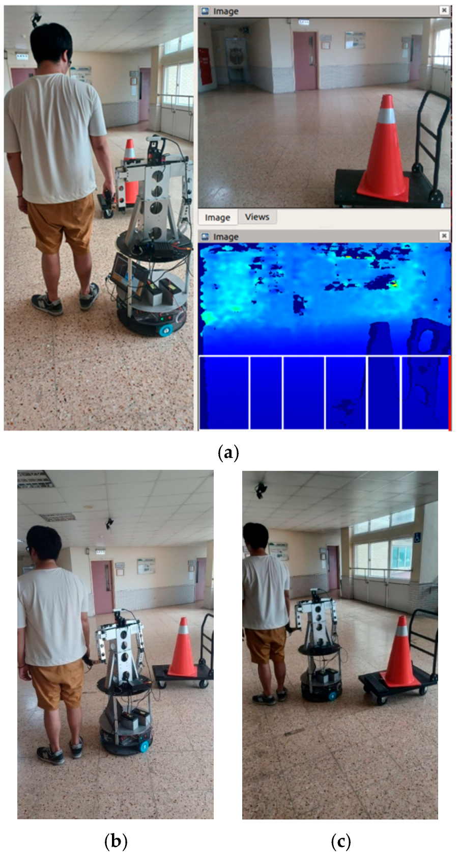
7.3. Avoid Obstacle
During the experiment, we predicted that we would encounter some unexpected obstacles. For this reason, we used the fuzzy theory to avoid static obstacles. In the stationary obstacle avoidance process, we used the depth camera to obtain the obstacle’s depth and position. Through the judgment of NVIDIA Jetson Xavier and according to the fuzzy rules, the corresponding instructions (turn left, turn right) were given to the motor, and the output time was controlled to achieve the obstacle avoidance function. After avoiding obstacles, it returned to the original path and continued to navigate until it encountered the next obstacle or reached the endpoint. In addition, when a dynamic obstacle is encountered, the depth is obtained using the depth camera, and the host can determine it. When any fuzzy rule cannot avoid the obstacle, the host will issue a stop command and stop the robot from moving forward. The robot will not continue until there are no obstacles in front of it. Figure 34 shows the process of static obstacle avoidance. Figure 35 shows the process of dynamic obstacle avoidance.

Figure 34.
The process of obstacle avoidance: (a) obstacle detected; (b) robot turns left; (c) robot passes the obstacle.
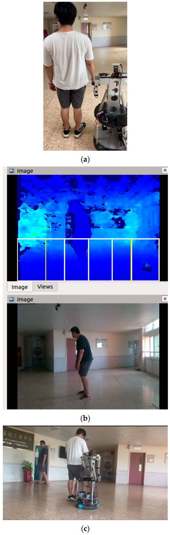
Figure 35.
The process of dynamic obstacle avoidance: (a) start moving; (b) stop moving forward when detecting dynamic obstacles; (c) start moving after the obstacles disappear.
The field of view of the depth camera is 65°. In obstacle environments, when the robot approaches an obstacle, at 100 cm away from the obstacle, the width in the real environment is 156 cm. The width of the camera image is divided into six boxes, each of which in the real environment is 26 cm. The fuzzy rules control the robot away from the obstacle, and the obstacle will be shifted at least one box away from the image center. Since the width of the robot is 40 cm, when passing by an obstacle, the robot will be at least 6 cm away from the obstacle. This ensures that the robot can avoid obstacles in any environment.
8. Conclusions
The primary purpose of this research is to help blind people by using robots to reduce obstacle collision while guiding them. The robot’s tasks are divided into two parts: (1) controlling the robotic arm close to the human hand, and (2) obstacle avoidance and path planning. For the first part, we used YOLOv5s as the object detection model. Compared to the YOLOv5 model, this model has a faster training speed, but relatively lower accuracy, but which can still meet our needs. For the control of the robotic arm, we used closed-loop control to obtain images using a depth camera. For the second part, we used D3QN as a path-planning method. This method has a better performance design for complex environments and is relatively intuitive because it allows for adjusting the reward and penalty values. However, its disadvantage is that it takes work to find the optimal parameters, which need to be solved by more intelligent algorithms. As for obstacle avoidance, we used fuzzy theory to avoid obstacles. The main reason for this is that its design is more straightforward than traditional PID control.
The experimental results show that some issues still need to be improved. One of the issues is the path planning part. Even though we used the genetic algorithm to define the optimal parameters for the path planning, there are still some differences in its measurements. The incompatibility of the hardware and software probably caused improper turning. We pursued speed while ignoring hardware matching when designing the system parameters. A second issue is that there was no reminder when encountering dynamic obstacles. In this experiment, we mainly achieved the purpose of a reminder by letting the robot stand still, and we did not design other protective measures. This is also a problem we must consider in the future. In this study, the roulette wheel selection was used for reproduction. Stochastic universal sampling might provide better performance in the reproduction process; this method will be used in our future work. In addition, we will implement alert systems, such as auditory or haptic feedback, to inform users when the robot avoids dynamic obstacles.
Supplementary Materials
The following supporting information can be downloaded at: https://www.mdpi.com/article/10.3390/machines13070560/s1. Figure S1. The Illustration of DQN; Figure S2. The Illustration of D3QN; Figure S3. Trajectories of x1 = 2, x2 = 1, x3 = 1; Figure S4. Trajectories of x1= 3, x2 = 1, x3 = 1; Figure S5. Trajectories of x1= 1, x2 = 1, x3 = 1; Figure S6. Trajectories of x1= 1, x2 = 3, x3 = 1; Figure S7. Trajectories of x1= 1, x2 = 1, x3 = 2; Figure S8. Trajectories of x1= 1, x2 = 1, x3 = 1; Figure S9. Fuzzy set.
Author Contributions
Conceptualization, J.-G.J.; Methodology, C.-H.Y. and J.-G.J.; Software, C.-H.Y.; Validation, C.-H.Y. and J.-G.J.; Formal analysis, C.-H.Y.; Investigation, J.-G.J.; Resources, J.-G.J.; Data curation, C.-H.Y.; Writing—original draft, C.-H.Y.; Writing—review & editing, J.-G.J.; Visualization, C.-H.Y.; Supervision, J.-G.J.; Project administration, J.-G.J.; Funding acquisition, J.-G.J. All authors have read and agreed to the published version of the manuscript.
Funding
The authors received no financial support for the research, authorship, and/or publication of this article.
Institutional Review Board Statement
Our institution did not require ethical approval for the fake blind people used in this study.
Data Availability Statement
Data are contained within the article.
Conflicts of Interest
The authors declared no potential conflicts of interest with respect to the research, authorship, and/or publication of this article.
References
- Kim, J.; Kang, B.Y.; Woo, J.W.; Baek, H. A Study on Evaluation Method for Indoor Guide Robot. In Proceedings of the 20th International Conference on Control, Automation and Systems, Busan, Republic of Korea, 13–16 October 2020; pp. 107–110. [Google Scholar]
- Azenkot, S.; Feng, C.; Cakmak, M. Enabling Building Service Robots to Guide Blind People: A Participatory Design Approach. In Proceedings of the 2016 ACM/IEEE International Conference on Human-Robot Interaction, Christchurch, New Zealand, 7–10 March 2016; pp. 3–10. [Google Scholar] [CrossRef]
- Katona, K.; Neamah, H.A.; Korondi, P. Obstacle Avoidance and Path Planning Methods for Autonomous Navigation of Mobile Robot. Sensors 2024, 24, 3573. [Google Scholar] [CrossRef] [PubMed]
- Dhananji, A.N.; Sharmilan, T. Autonomous Mobile Robot Navigation and Obstacle Avoidance: A Comprehensive Review. Eur. Mod. Stud. J. 2023, 7, 260–267. [Google Scholar] [CrossRef]
- Zhang, S. Development and Design of Tennis Obstacle Avoidance System Based on Machine Vision Technology. In Proceedings of the 2022 International Conference on Artificial Intelligence and Autonomous Robot Systems, Bristol, UK, 29–31 July 2022; pp. 153–157. [Google Scholar] [CrossRef]
- Tawil, Y.; Hafez, A.H.A. Deep Learning Obstacle Detection and Avoidance for Powered Wheelchair. In Proceedings of the 2022 Innovations in Intelligent Systems and Applications Conference, Antalya, Turkey, 7–9 September 2022; pp. 1–6. [Google Scholar] [CrossRef]
- Guo, B.; Guo, N.; Cen, Z. Obstacle Avoidance with Dynamic Avoidance Risk Region for Mobile Robots in Dynamic Environments. Proc. IEEE Robot. Autom. Lett. 2022, 7, 5850–5857. [Google Scholar] [CrossRef]
- Ruan, X.; Lin, C.; Huang, J.; Li, Y. Obstacle avoidance navigation method for robot based on deep reinforcement learning. In Proceedings of the 2022 IEEE 6th Information Technology and Mechatronics Engineering Conference, Chongqing, China, 4–6 March 2022; pp. 1633–1637. [Google Scholar] [CrossRef]
- Alarabi, S.; Luo, C.; Santora, M. A PRM Approach to Path Planning with Obstacle Avoidance of an Autonomous Robot. In Proceedings of the 2022 8th International Conference on Automation, Robotics, and Applications, Prague, Czech Republic, 18–20 February 2022; pp. 76–80. [Google Scholar] [CrossRef]
- Zhou, L.; Zhu, C.; Su, X. SLAM algorithm and Navigation for Indoor Mobile Robot Based on ROS. In Proceedings of the 2022 IEEE 2nd International Conference on Software Engineering and Artificial Intelligence, Xiamen, China, 10–12 June 2022; pp. 230–236. [Google Scholar] [CrossRef]
- Yang, X.; Yuxi, H.; Qiuhong, L. Robot path planning based on the improved grey wolf optimization algorithm. In Proceedings of the 2022 Power System and Green Energy Conference, Shanghai, China, 25–27 August 2022; pp. 543–547. [Google Scholar] [CrossRef]
- Muhammad, A.; Abdullah, N.R.H.; Ali, M.A.H.; Shanono, I.H.; Samad, R. Simulation Performance Comparison of A*, GLS, RRT, and PRM Path Planning Algorithms. In Proceedings of the 2022 IEEE 12th Symposium on Computer Applications & Industrial Electronics, Penang, Malaysia, 21–22 May 2022; pp. 258–263. [Google Scholar] [CrossRef]
- Pansare, A.; Sabu, N.; Kushwaha, H.; Srivastava, V.; Thakur, N.; Jamgaonkar, K.; Faiz, M.Z. Drone Detection using YOLO and SSD A Comparative Study. In Proceedings of the 2022 International Conference on Signal and Information Processing, Pune, India, 26–27 August 2022; pp. 1–6. [Google Scholar] [CrossRef]
- Intel RealSense LiDAR Camera D415. Available online: https://www.intelrealsense.com/depth-camera-d415/ (accessed on 7 July 2023).
- NVIDIA Jetson AGX Xavier. Available online: https://developer.nvidia.com/embedded/jetson-agx-xavier-developer-kit (accessed on 25 March 2023).
- Lin, T.Y. Application of 3D Point Cloud Map and Image Identification to Mobile Robot Control. Master Thesis, Department of Communications, Navigation and Control Engineering, NTOU, ROC, Keelung, Taiwan, 2021. [Google Scholar]
- Majumder, A. The Pinhole Camera. Available online: https://ics.uci.edu/~majumder/vispercep/cameracalib.pdf (accessed on 4 April 2023).
- Zhu, L. Improving YOLOv5 with Attention Mechanism for Detecting Boulders from Planetary Images. Remote Sens. 2021, 13, 3776. [Google Scholar] [CrossRef]
- YOLOv5s Architecture. Available online: https://medium.com/@_Xing_Chen_/yolov5-%E8%A9%B3%E7%B4%B0%E8%A7%A3%E8%AE%80-724d55ec774 (accessed on 8 April 2023).
- Robot Operating System. Available online: https://en.wikipedia.org/wiki/Robot_Operating_System (accessed on 12 April 2023).
- Chang, Y.T. Application of Depth Camera to Indoor Robot Control. Master Thesis, Department of Communications, Navigation and Control Engineering, NTOU, ROC, Keelung, Taiwan, 2022. [Google Scholar]
- Jiang, N.; Zhao, Q.; Wang, J. Deep Reinforcement Learning-based Path Planning Method for Underwater Gliders in Unknown 3D Marine Environment. Ships Offshore Struct. 2025, 20, 121–132. [Google Scholar] [CrossRef]
- Li, S.; Xu, X.; Zuo, L. Dynamic path planning of a mobile robot with improved Q-learning algorithm. In Proceedings of the 2015 IEEE International Conference on Information and Automation, Lijiang, China, 8–10 August 2015; pp. 409–414. [Google Scholar] [CrossRef]


Disclaimer/Publisher’s Note: The statements, opinions and data contained in all publications are solely those of the individual author(s) and contributor(s) and not of MDPI and/or the editor(s). MDPI and/or the editor(s) disclaim responsibility for any injury to people or property resulting from any ideas, methods, instructions or products referred to in the content. |
© 2025 by the authors. Licensee MDPI, Basel, Switzerland. This article is an open access article distributed under the terms and conditions of the Creative Commons Attribution (CC BY) license (https://creativecommons.org/licenses/by/4.0/).