Nonblocking Modular Supervisory Control of Discrete Event Systems via Reinforcement Learning and K-Means Clustering

Abstract

Traditional supervisory control methods for the nonblocking control of discrete event systems often suffer from exponential computational complexity. Reinforcement learning-based approaches mitigate state explosion by sampling many random sequences instead of computing the synchronous product of multiple modular supervisors, but they struggle with limited reachable state spaces. A primary novelty of this study is to use the K-means clustering method for online inference with the learned state-action values. The clustering method divides all events at a state into the good group and the bad group. The events in the good group are allowed by the supervisor. The obtained supervisor policy can ensure both system constraints and larger control freedom compared to conventional RL-based supervisors. The proposed framework is validated by two case studies: an industrial transfer line (TL) system and an automated guided vehicle (AGV) system. In the TL case study, nonblocking reachable states increase from 56 to 72, while in the AGV case study, a substantial expansion from 481 to 3558 states is observed. Our new method achieves a balance between computational efficiency and nonblocking supervisory control.

1. Introduction

Industrial automation requires multiple autonomous machines to work collaboratively to produce products with high productivity and safety. These machines include, for instance, assembly stations, mobile logistic vehicles, and storage buffers. The movement and operations of these machines must be coordinated by logic-level supervisory controllers. The supervisory control theory (SCT) [1,2] provides a theoretical framework for designing nonblocking and maximally permissive supervisors for discrete event systems (DESs). The supervisors may be designed by traditional exhaustive search methods or emerging sample-based methods using reinforcement learning (RL).

The traditional search-based methods suffer from exponential computational complexity. To reduce complexity, modular supervisory control [3] decomposes global specifications into multiple smaller local specifications, which are enforced by local modular supervisors [4]. Only the plant components that share events with the local specification are considered when designing the local modular supervisor. These supervisors collectively ensure compliance with the global specification. However, blocking states may appear in the controlled system due to the lack of coordination between independently designed local modular supervisors. A straightforward way to ensure nonblocking control is to introduce a coordinator to resolve the conflicting control decisions among modular supervisors. Nevertheless, the complexity of computing such a nonblocking coordinator can still grow exponentially with the number of supervisors and plant components. Developing coordination mechanisms that ensure nonblocking behavior with tractable computational complexity remains an open research question.

1.1. Traditional Methods for Coordinator Computing

Traditional SCT employs two primary strategies to efficiently achieve nonblocking modular supervisory control. The first strategy leverages the structural properties of the system to ensure that local modular supervisors maintain the nonblocking property. For instance, Feng and Wonham [5] propose the control-flow-network method, which analyzes the interactions among local supervisors and plant components. This method identifies specific network configurations that inherently guarantee nonblocking behavior for certain modular supervisors.These favorable network structures are common in manufacturing lines. In addition, Goorden et al. [6] present three structural properties that can be checked to verify nonblocking behavior in modular supervisory control applications.

The second strategy aims to alleviate computational complexity by employing system decomposition and hierarchical abstraction techniques in the coordinator synthesis process. This approach partitions the system into smaller, more manageable subsystems and abstracts their behavior into higher-level models, enabling efficient synthesis of a global supervisor. For instance, Schmidt et al. [7,8] propose a hierarchical abstraction technique that uses state aggregation to reduce the state space of individual modules while preserving their essential control properties. Their method significantly reduces the computational burden of synthesizing a coordinator, particularly in large-scale systems. Similarly, Leduc et al. [9] introduce a compositional synthesis framework that combines abstraction and decomposition to achieve scalable nonblocking control. Their approach leverages the concept of “partial models,” where each module is abstracted independently, and the global supervisor is synthesized incrementally. This method not only reduces computational complexity but also enhances the flexibility of the control method.

Recent advancements have further extended these strategies by integrating learning-based methods and formal verification tools. For instance, learning-based techniques are exploited for synthesizing modular supervisors in uncertain environments [10,11]. Additionally, tools like Supremica [12] and MIDES [13] have been developed to automate the synthesis and verification of modular supervisors, enabling the application of these strategies to industrial-scale systems. These developments highlight the ongoing evolution of SCT, where traditional strategies are being enhanced with modern computational techniques to address the challenges of increasingly complex systems.

1.2. RL-Based Methods

RL [14] has emerged as a promising alternative to traditional supervisory control methods in DESs. Traditional methods exhaustively search the state-transition model of the controlled system and prune unwanted states, but RL learns control policies through sample-based simulations of the target system. This sample-based approach effectively circumvents the state explosion problem commonly encountered in conventional coordinator design techniques. Kajiwara and Yamasaki [15] propose a RL-based approach for implementing supervisory control in decentralized DESs, where the central supervisor and local subsystems are characterized by distinct preference functions. The reward function is designed to account for both event occurrence and disabling during the learning process. Furthermore, Zielinski et al. [16] integrate SCT and RL to assign an optimal schedule to an industrial system, where SCT is utilized to build a safety search environment for RL algorithms. Hu et al. [17] combine SCT and RL to synthesize an optimal directed controller for a DES. Deep reinforcement learning (DRL) algorithms are incorporated into the above framework to effectively address control problems in large-scale DESs. Konishi et al. [18] integrate DRL and SCT to solve a safety control problem in DESs, where DRL algorithms are used to compute a suboptimal solution efficiently and SCT is employed to restrict the sub-optimal solution to a safety solution. Liu [10] combines SCT and RL to design nonblocking modular supervisors for DESs with unknown environments. Our previous research [19] employs SCT and DRL to compute a nonblocking coordinator for a set of local modular supervisors. Furthermore, SCT is employed to reduce the learning time of DRL for supervisor designing for DESs with linear temporal logic specifications [20].

1.3. Motivation and Contributions

Classical SCT strives for the supremal supervisor with the greatest reachable state set, but RL-based supervisors do not explicitly maximize the reachable state set. Hence, the RL-based supervisors are often limited in the reachable state space.

At a reachable state, a supervisor allows all uncontrollable events and a subset of controllable events. The cardinality of the controllable event subset is flexible, ranging from 0 to all controllable events. This flexibility helps the supervisor satisfy all control specifications and achieve the largest reachable state set. In contrast, RL algorithms choose only one action at a reachable state. This limitation significantly confines the reachable state set of the controlled systems. Our previous studies [19,20] attempt to enlarge the reachable state set of the RL-learned supervisor by selecting multiple actions, but these methods choose a fixed number of controllable events and incur longer training time. The flexibility of choosing an arbitrary number of controllable events at a reachable state is desirable for the RL-learned supervisor.

This paper adds this missed flexibility to RL-learned supervisors. Suppose that an RL algorithm maximizes the reward. After the learning process, the learned supervisor has evaluations for all pairs of reachable state and controllable events. If the supremal nonblocking supervisor allows a controllable event at a state, the evaluation number of the pair of state and event may be high. Otherwise, the evaluation of the pair may be low. A research hypothesis is that all events with higher evaluations learned by RL should be allowed by the supremal nonblocking supervisor. Since there is not a fixed threshold value for dichotomizing the controllable events, we apply the clustering method to identify the pattern of the events and choose the flexible group of allowed events. Among clustering algorithms like hierarchical clustering [21], support vector machine [22], a density-based method [23], and fuzzy C-Means [24], K-means [25] emerges as the most suitable choice for this study because its simplicity and computational efficiency align with the binary classification requirement of evaluation numbers.

We evaluate the proposed method with a transfer line system and an automated guided vehicle (AGV) system. The results show that the proposed method greatly enlarges the state size of the controlled system, compared with the method only using RL. The structure of the paper is as follows. Section 2 reviews the necessary preliminaries. The research problem and its solution are presented in Section 4. Section 5 demonstrates the implementation of the proposed method and Section 6 concludes the paper.

2. Preliminaries

2.1. Deterministic Finite Automata (DFA)

A DFA is formally represented as a five-tuple $\mathbf{G}=\langle Q,\Sigma ,\eta ,q_0,Q_m\rangle$, where:

• Q denotes a finite, nonempty set of states;
• $\Sigma$ is a finite, nonempty alphabet representing the set of event labels;
• $\eta :Q\times \Sigma \to Q$ is a (partially defined) transition function;
• $q_0\in Q$ is the designated initial state;
• $Q_m\subseteq Q$ represents the set of marker (or accepting) states.

For a state $q\in Q$ and an event $\sigma \in \Sigma$, denote $\eta (q,\sigma )!$ if $\eta (q,\sigma )$ is defined. The set of events that are defined at q is $Enb\left(q\right)=\{\sigma \in \Sigma \mid \eta (q,\sigma )!\}$; q is a deadlock state if $Enb\left(q\right)=\varnothing$.

An event reward function $R_e:\Sigma \to \mathbb{R}$ and a state reward function $R_s:Q\to \mathbb{R}$ are defined for DESs as follows. For an event $\sigma \in \Sigma$,

$$R_e\left(\sigma \right)=\left\{\begin{array}{cc}{w}_1,\hfill & \mathrm{if}\sigma \in {\Sigma }_s\hfill \\ 0,\hfill & \mathrm{otherwise},\hfill \end{array}\right.$$

(1)

where ${\Sigma }_s\subseteq \Sigma$ defines a specific event set, and $w_1$ is a positive real number. For a state $q\in Q$,

$$R_s\left(q\right)=\left\{\begin{array}{cc}{w}_1,\hfill & \mathrm{if}q\in Q_m\hfill \\ w_2,\hfill & \mathrm{if}q\notin Q_m\&Enb\left(q\right)=\varnothing \hfill \\ 0,\hfill & \mathrm{otherwise},\hfill \end{array}\right.$$

(2)

where $w_2$ is a negative real number.

2.2. SCT and Local Modular Supervisors

A plant in SCT is modeled as a DFA $\mathbf{G}$, whose event set $\Sigma$ is partitioned into controllable event set ${\Sigma }_c$ and uncontrollable event set ${\Sigma }_u$. The specification of the plant behavior is described by another DFA $\mathbf{E}$, whose event set is also $\Sigma$. A supervisory controller is designed to ensure the plant satisfies the desired requirements by disabling some controllable events. The supervisory control function is $V:Q\to \mathcal{C}$, where $\mathcal{C}=\{\Pi \subseteq \Sigma |{\Sigma }_u\subseteq \Pi \}$ denotes the set of all event subsets that may be enabled at a given system state. Note that uncontrollable events are always permitted to occur. At a system state $q\in Q$, the supervisory control function determines a permissible event set $V\left(q\right)$, and all events not in $V\left(q\right)$ are disabled. Consequently, the closed-loop behavior of the plant $\mathbf{G}$ is constrained to a subset of the intersection of the behaviors of the plant $\mathbf{G}$ and the specification $\mathbf{E}$, and the closed-loop behavior is nonblocking. SCT synthesizes a maximally permissive supervisor ${\mathbf{S}}^{*}$ that permits the greatest reachable state set of the closed-loop behavior.

Many DES control problems involve multiple concurrent plant components and modular control specifications. Let ${\mathbf{G}}_i(i\in 1,\dots ,b)$ and ${\mathbf{E}}_j(j\in 1,\dots ,d)$ denote the DFAs modeling the i-th plant component and the j-th specification, respectively, each defined over event sets ${\Sigma }_i$ and ${\Sigma }_j^{\prime }$. Here, b and d are integers greater than one. The set of plant components that interact with specification ${\mathbf{E}}_j$ is given by $\mathit{Share}\left({\mathbf{E}}_j\right)=\{i\in 1,\dots ,b\mid {\Sigma }_i\cap {\Sigma }_j^{\prime }\ne \varnothing \}$. The synchronous product of two DFAs is defined as follows. Given two DFAs ${\mathbf{G}}_1=\langle Q_1,{\Sigma }_1,{\eta }_1,q_{10},Q_{1m}\rangle$ and ${\mathbf{G}}_2=\langle Q_2,{\Sigma }_2,{\eta }_2,q_{20},Q_{2m}\rangle$, their synchronization is ${\mathbf{G}}_1\parallel {\mathbf{G}}_2=\langle Q,\Sigma ,\eta ,q,Q_m\rangle$, where

• $Q=Q_1\times Q_2$ is the state set;
• $\Sigma ={\Sigma }_1\cup {\Sigma }_2$ is the set of events;
• $\eta :Q\times \Sigma \to Q$ is the partial transition function. For $q=(q_1,q_2)\in Q$ and $\sigma \in \Sigma$,

  $$\begin{array}{c}\hfill \eta (q,\sigma )=\left\{\begin{array}{cc}(q_1^{\prime },q_2),\hfill & \mathrm{if}\sigma \in {\Sigma }_1-{\Sigma }_2,q_1^{\prime }={\eta }_1(q_1,\sigma )\hfill \\ (q_1,q_2^{\prime }),\hfill & \mathrm{if}\sigma \in {\Sigma }_2-{\Sigma }_1,q_2^{\prime }={\eta }_2(q_2,\sigma )\hfill \\ (q_1^{\prime },q_2^{\prime }),\hfill & \mathrm{if}\sigma \in {\Sigma }_1\cap {\Sigma }_2,q_1^{\prime }={\eta }_1(q_1,\sigma ),q_2^{\prime }={\eta }_2(q_2,\sigma )\hfill \\ \mathrm{undefined},\hfill & \mathrm{otherwise};\hfill \end{array}\right.\end{array}$$
• $q_0=(q_{10},q_{20})$ is the initial state;
• $Q_m=Q_{1m}\times Q_{2m}$ is the set of marker states.

The operation can be extended to more than two DFAs. For each specification ${\mathbf{E}}_j$, the associated local plant is constructed as ${\mathbf{H}}_j{=\Vert }_{i\in \mathit{Share}\left({\mathbf{E}}_j\right)}{\mathbf{G}}_i$. The corresponding modular supervisor ${\mathbf{S}}_j$, which enforces the specification ${\mathbf{E}}_j$, is computed from the composition of ${\mathbf{H}}_j$ and ${\mathbf{E}}_j$ using SCT [26,27]. Consequently, the concurrent behavior of all plant components ${\mathbf{G}}_i=\langle Q_i,{\Sigma }_i,{\eta }_i,q_{i0},Q_{im}\rangle$ satisfies all specifications under the supervisory control of ${\mathbf{S}}_j=\langle Y_j,\Sigma ,{\delta }_j,y_{j0},Y_{jm}\rangle$. The overall behavior of the controlled DES is captured by the synchronous composition of all local modular supervisors along with their respective plant models. As noted in Section 1, the controlled DES may exhibit blocking behavior, which necessitates a coordinator to guarantee nonblocking execution [1,28].

2.3. Optimal Controller for the Markov Decision Process

A Markov decision process (MDP) is formally represented as a five-tuple $\mathcal{M}=\langle S,\mathcal{A},\mathcal{T},s_0,\mathcal{R}\rangle$:

• S denotes a finite state space containing at least one state;
• $\mathcal{A}$ represents the finite set of available actions;
• $\mathcal{T}:S\times \mathcal{A}\times S\to [0,1]$ specifies state transition probabilities;
• $s_0\in S$ identifies the initial system state;
• $\mathcal{R}:S\times \mathcal{A}\times S\to \mathbb{R}$ defines the step reward function.

Within this framework, a deterministic control policy maps states to actions through a function $\pi :S\to \mathcal{A}$. Implementing policy $\pi$ on $\mathcal{M}$ generates a Markov chain ${\mathcal{M}}_{\pi }$ with transition probabilities $\mathcal{T}(s,\pi \left(s\right),s^{\prime })$ between states s and $s^{\prime }$. The system’s evolution under this policy produces infinite trajectories $\tau =(s_0,a_0,s_1),(s_1,a_1,s_2),\dots$ where each transition satisfies $\mathcal{T}(s_i,a_i,s_{i+1})>0$ with $a_i=\pi \left(s_i\right)$.

The cumulative discounted return for trajectory $\tau$ is calculated as:

$$G\left(\tau \right)=\sum _{k=0}^{\infty }{\gamma }^k\mathcal{R}(s_k,a_k,s_{k+1})$$

(3)

where $\gamma \in (0,1]$ serves as the discount factor, progressively diminishing the impact of future rewards. The state-value function $V_{\pi }:S\to \mathbb{R}$ quantifies the expected cumulative discounted return from state s:

$$V_{\pi }\left(s\right)={\mathbb{E}}_{\pi }\left[G\left(\tau \right)\mid s_0=s\right]$$

(4)

Following Bellman’s principle of optimality [14], this value function satisfies the recursive relationship:

$$V_{\pi }\left(s\right)=\sum _{s^{\prime }\in S}\mathcal{T}(s,\pi \left(s\right),s^{\prime })\left[\mathcal{R}(s,\pi \left(s\right),s^{\prime })+\gamma V_{\pi }\left(s^{\prime }\right)\right]$$

(5)

The optimal control policy ${\pi }^{*}$ maximizes expected returns across all states:

$${\pi }^{*}=\underset{\pi }{argmax}\sum _{s^{\prime }\in S}\mathcal{T}(s,\pi \left(s\right),s^{\prime })\left[\mathcal{R}(s,\pi \left(s\right),s^{\prime })+\gamma V_{\pi }\left(s^{\prime }\right)\right]$$

(6)

There are two main approaches to determining ${\pi }^{*}$: model-based methods using dynamic programming when full knowledge of $\mathcal{T}$ and $\mathcal{R}$ is available, and model-free reinforcement learning methods when transition dynamics are unknown.

2.4. K-Means Clustering

K-means clustering [25] is a popular unsupervised learning algorithm designed to partition a dataset into multiple disjoint clusters based on similarity. The method iteratively assigns data points to clusters and refines the cluster centers to minimize the variance within each cluster. Hence, similar data points are effectively grouped together. Mathematically, given a dataset $U=\{u_i\in {\mathbb{R}}^m\mid i=1,\dots ,n\}$, K-means aims to partition it into k clusters $\mathbf{C}=\{C_1,\dots ,C_k\}$ to minimize the sum of within-cluster variances:

$$\underset{\mathbf{C}}{min}\sum _{C_l\in \mathbf{C}}\sum _{u_i\in C_l}{\Vert u_i-{\mu }_l\Vert }^2,$$

(7)

subject to

$${\mu }_l={\displaystyle \frac{1}{\mid C_l\mid }}\sum _{u_i\in C_l}{u}_i,$$

(8)

$$C_l\cap C_p=\varnothing ,l\ne p,l,p\in \{1,\dots ,k\}$$

$${\cup }_{l=1}^k{C}_l=U$$

where ${\mu }_l$ is the centroid of cluster $C_l$ and $\Vert ·\Vert$ represents the Euclidean norm.

The K-means algorithm first randomly selects k centroids from the dataset. It then calculates the distance of each data point to all chosen centroids and assigns each point to the cluster of the nearest centroid. When a data point is added to a cluster, the cluster’s centroid is recalculated. This process repeats iteratively until the cluster assignments converge.

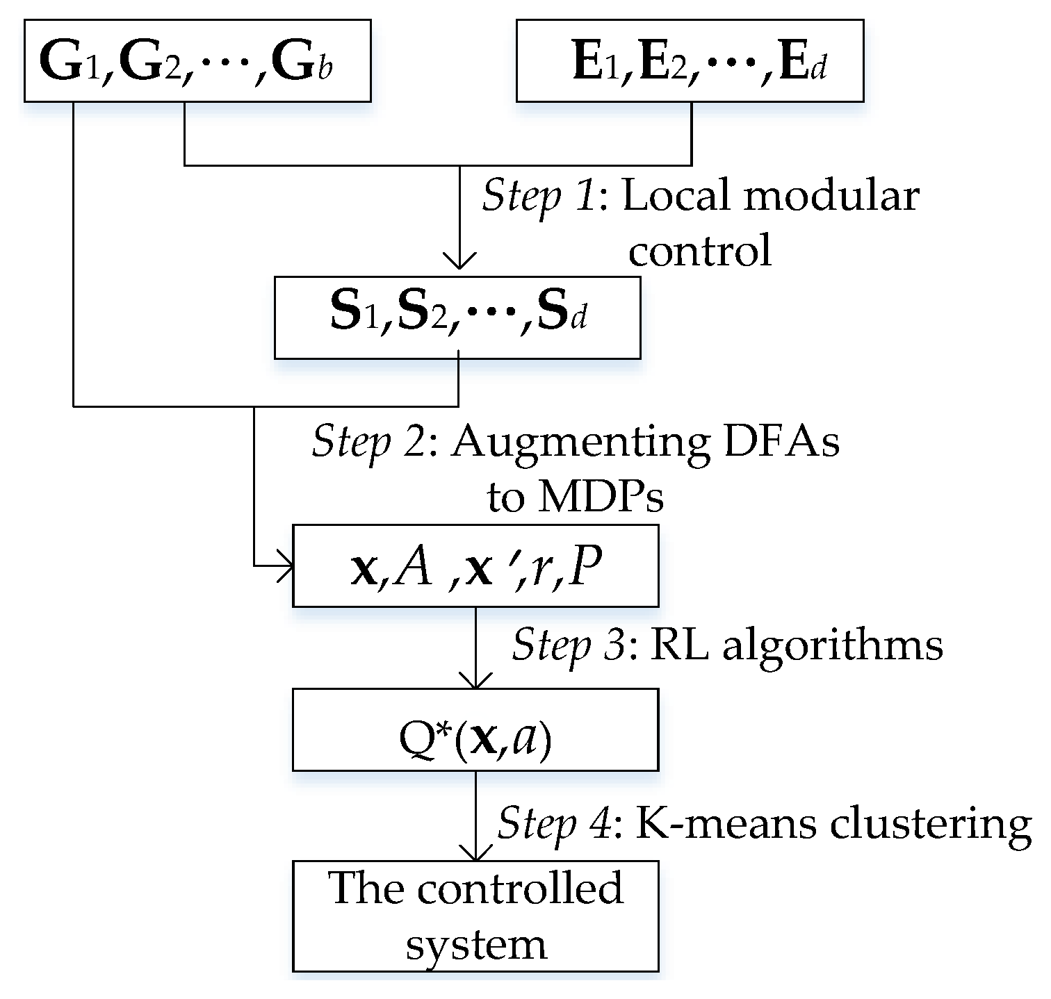
3. Schema of the Overall Approach

The proposed methodology for nonblocking modular supervisory control follows a structured four-step process, as illustrated in Figure 1. Step 1 uses the plant models $\{{\mathbf{G}}_1,{\mathbf{G}}_2,\dots ,{\mathbf{G}}_b\}$ and specification models $\{{\mathbf{E}}_1,{\mathbf{E}}_2,\dots ,{\mathbf{E}}_d\}$ to synthesize a group of local modular supervisors $\{{\mathbf{S}}_1,{\mathbf{S}}_2,\dots ,{\mathbf{S}}_d\}$. Step 2 augments the obtained DFAs to MDPs, according to the method elaborated in Section 4. Step 3 applies the Q learning algorithm to learn the optimal state-action value function $Q^{*}(\mathbf{x},a)(a\in A)$, which evaluates the reward value for every state and action pair $(\mathbf{x},a)$. Step 4 uses K-means clustering to infer the allowed event subset at the current state.

4. Combination of SCT, RL, and K-Means Clustering

We propose a procedure that combines SCT, RL, and K-means clustering to compute supervisory controllers that meet control requirements, ensure nonblocking property, and allow close-to-optimal freedom. Let ${\mathbf{G}}_i(i=1,\dots ,b)$ and ${\mathbf{E}}_j(j=1,\dots ,d)$ represent the DFA models of the i-th plant component and the j-th requirement, respectively. For the specification ${\mathbf{E}}_j$, the associated local plant is computed as ${\mathbf{H}}_j{=\Vert }_{i\in \mathit{Share}\left({\mathbf{E}}_j\right)}{\mathbf{G}}_i$. The nonblocking local modular supervisor ${\mathbf{S}}_j=\langle Y_j,{\Sigma }_j,{\delta }_j,q_{j0},Y_{jm}\rangle$ is synthesized by SCT from ${\mathbf{H}}_j$ and ${\mathbf{E}}_j$. As a result, d local modular supervisors are derived. Consequently, the controlled system under the local modular supervisors is described by a compositional DFA $\mathbf{G}=\langle \mathbf{X},\Sigma ,\Delta ,{\mathbf{x}}_0,{\mathbf{X}}_m\rangle$, where $\mathbf{X}$ and ${\mathbf{X}}_m$ are collections of global states and global marker states, respectively.

As introduced in [19], a global state $\mathbf{x}=(q_1,q_2,\dots ,q_b,y_1,y_2,\dots ,y_d)\in \mathbf{X}$ of the system contains states of all plant components and local modular supervisors; $\mathbf{x}\in {\mathbf{X}}_m$ is called a global marker state if $(\forall i\in \{1,\dots ,b\},\forall j\in \{1,\dots ,d\})q_i\in Q_{im}\wedge y_j\in Y_{jm}$. The initial global state is ${\mathbf{x}}_0=(q_{10},\dots ,q_{b0},y_{10},\dots ,y_{d0})$. Define the index function $I:\Sigma \to 2^{\{1,\dots ,b\}}$ to determine the indexes of the plant components that contain a given event. For an event $\sigma \in \Sigma$, $I\left(\sigma \right)=\{i\in \{1,\dots ,b\}|\sigma \in {\Sigma }_i\}$. An event $\sigma \in \Sigma$ is allowed to occur at a global state $\mathbf{x}$, namely, $\Delta (\mathbf{x},\sigma )!$, if $(\forall i\in I\left(\sigma \right)){\eta }_i(q_i,\sigma )!\wedge (\forall j\in \{1,\dots ,d\}){\delta }_j(y_j,\sigma )!$. The set of all allowed events at state $\mathbf{x}$ is $Enb\left(\mathbf{x}\right)=\{\sigma \in \Sigma \mid \Delta (\mathbf{x},\sigma )!\}$. If $Enb\left(\mathbf{x}\right)=\varnothing$, then $\mathbf{x}$ is called a deadlock state. After an event $\sigma \in Enb\left(\mathbf{x}\right)$ occurs at state $\mathbf{x}$, the DES reaches the next global state ${\mathbf{x}}^{\prime }=\Delta (\mathbf{x},\sigma )=(q_1^{\prime },q_2^{\prime },\dots ,q_b^{\prime },y_1^{\prime },y_2^{\prime },\dots ,y_d^{\prime })$, where $(\forall i\in I\left(\sigma \right))q_i^{\prime }={\eta }_i(q_i,\sigma )\wedge (\forall i\notin I\left(\sigma \right))q_i^{\prime }=q_i\wedge (\forall j\in \{1,\dots ,d\})y_j^{\prime }={\delta }_j(y_j,\sigma )$.

4.1. Augmenting DFAs to MDPs

This part constructs an MDP from the obtained DFA $\mathbf{G}=\langle \mathbf{X},\Sigma ,\Delta ,{\mathbf{x}}_0,{\mathbf{X}}_m\rangle$ and computes the evaluations for all pairs of reachable state and controllable events for the following K-means clustering step. Since only controllable events can be disabled in SCT, the action set is defined as

$$A={\Sigma }_c$$

(9)

to suit the RL framework. As introduced in Section 2.2, a supervisor of $\mathbf{G}$ decides a subset of allowed events $\Pi \in \mathcal{C}$ at every reachable state $\mathbf{x}$. To apply RL methods to obtain the event subset, we define a mapping $\pi :A\to \mathcal{C}$ that maps an action to an event subset. For an action $a\in A$, define

$$\pi \left(a\right)=\left\{a\right\}\cup {\Sigma }_u$$

(10)

If the agent chooses action $a\in A$ at a global state $\mathbf{x}$, there must be one controllable event that is permitted. As a result, each controllable event at a reachable state has a evaluation value after training. In addition, a none controllable event is allowed at this state if the evaluations of all controllable events at $\mathbf{x}$ do not satisfy the section condition. Define the function $\Psi :\mathbf{X}\times A\to 2^{\Sigma }$ as

$$\Psi (\mathbf{x},a)=\pi \left(a\right)\cap Enb\left(\mathbf{x}\right)$$

(11)

to get all executable events at state $\mathbf{x}$ for action a.

Since an arbitrary event in $\Psi (\mathbf{x},a)$ may occur, the next state is uncertain. This implies that, after the introduction of the action set A, the global DFA obtained becomes stochastic for the RL agent and can hence be considered as an MDP $\mathbf{M}=\langle \mathbf{X},A,P,{\mathbf{x}}_0,r\rangle$ for the RL agent, where the state transition probability function is $P:\mathbf{X}\times A\times \mathbf{X}\to [0,1]$. For a global state $\mathbf{x}$ and an action $a\in A$, if $\Psi (\mathbf{x},a)=\varnothing$, then for any next global state ${\mathbf{x}}^{\prime }$, the state transition probability is $P(\mathbf{x},a,{\mathbf{x}}^{\prime })=0$. Otherwise, we derive the probability value $P(\mathbf{x},a,{\mathbf{x}}^{\prime })$ from the assumption that any event in the allowed event subset $\Psi (\mathbf{x},a)$ has an equal chance to occur, i.e., $(\forall \sigma \in \Psi (\mathbf{x},a\left)\right)$$Pr\left(\sigma \right|\mathbf{x},a)={\displaystyle \frac{1}{|\Psi (\mathbf{x},a\left)\right|}}$. The uniform event occurrence probability assumption is verified in [19] by a case study. The results show that this assumption does not affect the nonblocking property of the controlled system and the majority of the episode rewards based on the uniform distribution are bigger than those based on the non-uniform probability distribution.

Furthermore, a function is defined as $E:\mathbf{X}\times A\times \mathbf{X}\to 2^{\Sigma }$, such that

$$E(\mathbf{x},a,{\mathbf{x}}^{\prime })=\{\sigma \in \Psi (\mathbf{x},a)|\Delta (\mathbf{x},\sigma )={\mathbf{x}}^{\prime }\}$$

(12)

to collect the events that can reach ${\mathbf{x}}^{\prime }$ from $\mathbf{x}$ by action a. The probability value $P(\mathbf{x},a,{\mathbf{x}}^{\prime })$ is the cardinality of $E(\mathbf{x},a,{\mathbf{x}}^{\prime })$ divided by the number of all events in $\Psi (\mathbf{x},a)$, i.e.,

$$P(\mathbf{x},a,{\mathbf{x}}^{\prime })={\displaystyle \frac{\left|E\right(\mathbf{x},a,{\mathbf{x}}^{\prime }\left)\right|}{|\Psi (\mathbf{x},a\left)\right|}}$$

(13)

Evidently, if ${\mathbf{x}}^{\prime }\notin \Delta (\mathbf{x},\pi \left(a\right))$, then $P(\mathbf{x},a,{\mathbf{x}}^{\prime })=0$, where $\Delta (\mathbf{x},\pi \left(a\right))=\{{\mathbf{x}}^{\prime }\mid {\mathbf{x}}^{\prime }=\Delta (\mathbf{x},\sigma ),\sigma \in \pi \left(a\right)\}$.

The step reward function $r:\mathbf{X}\times A\times \mathbf{X}\to \mathbb{R}$ for the MDP is defined based on Equations (1) and  (2). For a step from $\mathbf{x}$ to ${\mathbf{x}}^{\prime }$ by action $a\in A$, $r(\mathbf{x},a,{\mathbf{x}}^{\prime })=0$ if $E(\mathbf{x},a,{\mathbf{x}}^{\prime })=\varnothing$. Otherwise,

$$r(\mathbf{x},a,{\mathbf{x}}^{\prime })={\displaystyle \frac{1}{\left|E\right(\mathbf{x},a,{\mathbf{x}}^{\prime }\left)\right|}}\sum _{\sigma \in E(\mathbf{x},a,{\mathbf{x}}^{\prime })}{R}_e\left(\sigma \right)+R_s\left({\mathbf{x}}^{\prime }\right)$$

(14)

According to  (6), the optimal controller $f^{*}$ for MDP $\mathbf{M}=\langle \mathbf{X},A_o,P,{\mathbf{x}}_0,r\rangle$ is computed by

$$f^{*}=arg\underset{f}{max}\sum _{{\mathbf{x}}^{\prime }\in \Delta (\mathbf{x},\Psi (\mathbf{x},f\left(\mathbf{x}\right)))}P(\mathbf{x},f\left(\mathbf{x}\right),{\mathbf{x}}^{\prime })[r(\mathbf{x},f\left(\mathbf{x}\right),{\mathbf{x}}^{\prime })+\lambda U_f\left({\mathbf{x}}^{\prime }\right)]$$

(15)

where $\Delta (\mathbf{x},\Psi (\mathbf{x},f\left(\mathbf{x}\right)))=\{{\mathbf{x}}^{\prime }\mid {\mathbf{x}}^{\prime }=\Delta (\mathbf{x},\sigma ),\sigma \in \Psi (\mathbf{x},f\left(\mathbf{x}\right))\}$. To employ Q learning, a state-action value function $Q_f:\mathbf{X}\times A\to \mathbb{R}$ for the controller f is defined to replace $U_f$ in the learning process. Executing an action $a\in A$ at a global state $\mathbf{x}$, the expected return is

$$\begin{array}{cc}\hfill Q_f(\mathbf{x},a)& =\sum _{{\mathbf{x}}^{\prime }\in \Delta (\mathbf{x},\Psi (\mathbf{x},a))}P(\mathbf{x},a,{\mathbf{x}}^{\prime })[r(\mathbf{x},a,{\mathbf{x}}^{\prime })+\lambda U_f\left({\mathbf{x}}^{\prime }\right)]\hfill \\ \hfill & ={\displaystyle \frac{1}{\mid \Psi (\mathbf{x},a)\mid }}\sum _{\sigma \in \Psi (\mathbf{x},a)}{R}_e\left(\sigma \right)+R_s(\Delta (\mathbf{x},\sigma )+\lambda U_f(\Delta (\mathbf{x},\sigma ))\hfill \end{array}$$

(16)

The optimal Q function is

$$Q^{*}(\mathbf{x},a)={\displaystyle \frac{1}{\mid \Psi (\mathbf{x},a)\mid }}\sum _{\sigma \in \Psi (\mathbf{x},a)}{R}_e\left(\sigma \right)+R_s(\Delta (\mathbf{x},\sigma ))+\lambda \underset{a^{\prime }}{max}{Q}^{*}(\Delta (\mathbf{x},\sigma ),a^{\prime })$$

(17)

under the optimal control function $f^{*}$.

To evaluate and improve the learning performance, the concept of temporal difference (TD) [14] is introduced. Temporal difference methods enable the agent to learn optimal value functions incrementally by comparing estimates across successive states. Specifically, the TD error measures the discrepancy between the predicted value of the current state-action pair and the updated estimate based on subsequent states. For employing the Q learning algorithm, the temporal difference error is defined as

$$T{D}_{error}={\displaystyle \frac{1}{\mid \Psi (\mathbf{x},a)\mid }}\sum _{\sigma \in \Psi (\mathbf{x},a)}[R_e\left(\sigma \right)+R_s(\Delta (\mathbf{x},\sigma ))+\lambda \underset{a^{\prime }}{max}Q(\Delta (\mathbf{x},\sigma ),a^{\prime })]-Q(\mathbf{x},a)$$

(18)

Consequently,

$$Q(\mathbf{x},a)\leftarrow Q(\mathbf{x},a)+\alpha \times T{D}_{error}$$

(19)

where $\alpha$ denotes the learning rate and regulates the learning speed. By incorporating the temporal difference, the RL agent learns to approximate the optimal Q-function efficiently.

Algorithm 1 outlines the RL algorithm employed in this paper. Each episode begins with the initial global state ${\mathbf{x}}_0$ and terminates if the maximal step is arrived or no event is available at the reached state, i.e., $Enb\left(\mathbf{x}\right)=\varnothing$. Note that the second termination condition includes two situations. First, the terminal state is a marker state that qualifies a positive state reward $w_1$. Second, the terminal state is indeed a deadlock state and deserves a negative number $w_2$. The exploration–exploitation trade-off is managed using the method named $ϵ—$greedy strategy, where $ϵ\in (0,1)$. At the end of each episode at Line 25, $ϵ$ is reduced but the minimal value is 0.01. At a global state $\mathbf{x}$, the algorithm randomly selects an action $a\in A$ with probability $ϵ$ or chooses the action $a=arg\underset{a}{max}{Q}^{*}(\mathbf{x},a)$.

The event subset decided at $\mathbf{x}$ by the chosen action a is $\Psi (\mathbf{x},a)$. If $\Psi (\mathbf{x},a)=\varnothing$, meaning that the controllable event selected is not defined at $\mathbf{x}$, the state-action value is updated in Line 13, where a negative real number $w_2$ is assigned as a penalty for this selection. The current state is then retained as the next state to facilitate sufficient exploration during the learning process in this situation. Conversely, if $\Psi (\mathbf{x},a)\ne \varnothing$, we consider the transitions caused by all events in $\Psi (\mathbf{x},a)$ and update the Q function as Equation (19). In this scenario, the next state is arbitrarily chosen from the set of reachable states $\Delta (\mathbf{x},\Psi (\mathbf{x},a\left)\right)$.

Algorithm 1 is developed for finite state MDPs, and its convergence is guaranteed according to [29]. Moreover, the reward generated in one episode, the episode number, and the average reward over the previous $\mathit{Len}$ episodes are denoted by $\mathit{EpReward},\mathit{EpR}$, and $\mathit{AvR}$, respectively. The iteration terminates when either $\mathit{AvR}$ exceeds the threshold e or $\mathit{EpNum}$ surpasses the maximum allowed limit $\mathit{MaxEp}$. At this point, the converged state-action table $Q(\mathbf{x},a)$ is returned. To track the mean reward over the most recent $\mathit{Len}$ episodes, an empty circular buffer $\mathit{Que}$ of size $\mathit{Len}$ is initialized. After each episode completes, the obtained reward is inserted into $\mathit{Que}$.

4.2. Online Inference by K-Means Clustering

Algorithm 1 provides the learned Q function values, where each reachable state and controllable event pair is associated with a value, $Q^{*}(\mathbf{x},a)$. This section focuses on computing the final supervisor by employing the K-means clustering algorithm for online inference. The goal is to map each reachable state to a permissible event subset based on the Q function values. At a reachable state $\mathbf{x}$, the set of Q function values for controllable events is expressed as

$$U\left(\mathbf{x}\right)=\{Q^{*}(\mathbf{x},a)\mid a\in A\}$$

(20)

Algorithm 1: Q-learning for computing state-action values

Data: $\mathbf{M}=\langle \mathbf{X},A_o,P,{\mathbf{x}}_0,r\rangle$, $\lambda$, $\alpha$, $ϵ$, $\mathit{dec}$, e, $\mathit{MaxSt}$, $\mathit{MaxEp}$ and $\mathit{Len}$

Result: A converged state-action table $Q(\mathbf{x},a)$

The K-means clustering algorithm, as discussed in Section 2.4, is applied to partition $U\left(\mathbf{x}\right)$ into two clusters, $C_1$ and $C_2$, such that $min\left(C_1\right)>max\left(C_2\right)$. The cluster with larger values, $C_1$, corresponds to the set of allowed actions at $\mathbf{x}$. This resulting action set is

$$A_1=\{a\mid Q^{*}(\mathbf{x},a)\in C_1\}$$

(21)

Since each action corresponds to a controllable event, $A_1$ is the permitted controllable event subset at $\mathbf{x}$. Finally, the allowed event subset at $\mathbf{x}$ is $(A_1\cup {\Sigma }_u)\cap Enb\left(\mathbf{x}\right)$. This method ensures that the permissible event set incorporates actions with high evaluation values while also considering all defined uncontrollable events.

Algorithm 2 computes the permissible event subset $\gamma$ for a given state $\mathbf{x}$ based on the learned Q function. The process leverages variance analysis and K-means clustering to determine whether or not clustering is necessary and to enlarge the set of controllable events if appropriate. The algorithm requires three inputs: the current state $\mathbf{x}$, the learned Q function values $Q^{*}(\mathbf{x},a)$ for all actions $a\in A$, and a predefined threshold $\delta \in [0,1]$. The value set $U\left(\mathbf{x}\right)$ is computed as Equation (20) at $\mathbf{x}$. If all values are less than zero, it indicates that all controllable events lead to deadlock states. In this case, no controllable events are permitted, and the event subset $\gamma$ includes only the defined uncontrollable events. Otherwise, $\delta$ is used to determine the partition of controllable events. To eliminate manual parameter recalibration for threshold $\delta$ across datasets with differing magnitudes, values at $\mathbf{x}$ are normalized as

$$U_{norm}\left(\mathbf{x}\right)=\{{\displaystyle \frac{Q^{*}(\mathbf{x},a)-U_{min}}{U_{max}-U_{min}}}\mid a\in A\}$$

(22)

where $U_{max}$ and $U_{min}$ represent the maximum and minimum of $U\left(\mathbf{x}\right)$, respectively. Let $u_i$ be the i-th element of $U_{norm}\left(\mathbf{x}\right)$. The standard deviation ${\sigma }_{norm}$ is calculated as

$${\sigma }_{norm}=\sqrt{{\displaystyle \frac{1}{\mid A\mid }}\sum _{i=1}^{\mid A\mid }{\left(u_i-\overline{u}\right)}^2}$$

(23)

where

$$\overline{u}={\displaystyle \frac{1}{\mid A\mid }}\sum _{i=1}^{\mid A\mid }{u}_i$$

(24)

If ${\sigma }_{norm}<\delta$, the variance is deemed insignificant. All controllable events are permitted, and the permissible event subset includes the defined controllable and uncontrollable events at the current state. If ${\sigma }_{norm}\ge \delta$, K-means clustering is applied to divide $U\left(\mathbf{x}\right)$ into two clusters. The actions corresponding to the cluster $C_1$ with larger estimation values are used to construct the permissible event subset, and the event subset $\gamma$ is computed in Line 11.

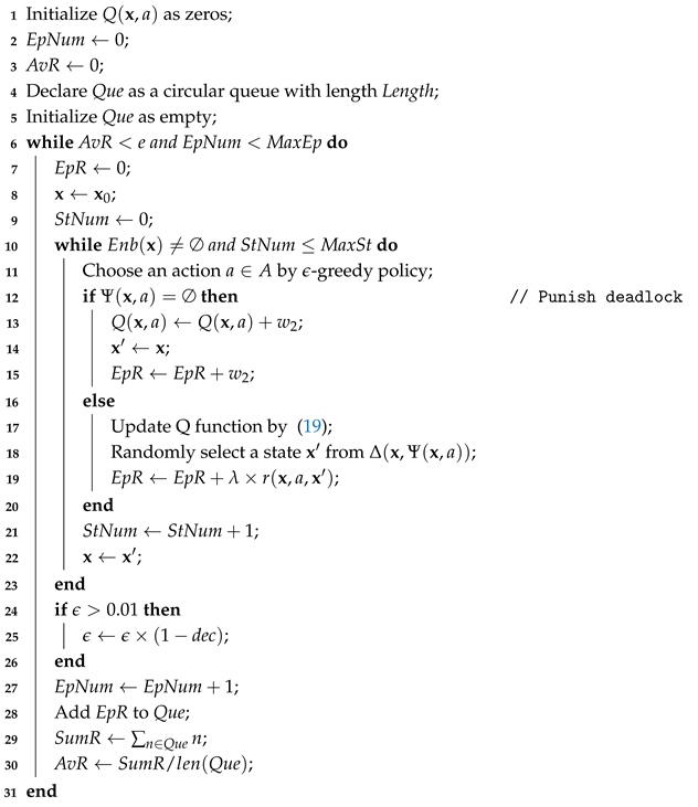
Algorithm 2: Computing the permitted event subset at $\mathbf{x}$ based on $Q^{*}(\mathbf{x},a)$ and K-means clustering

Data: The learned Q-function $Q^{*}(\mathbf{x},a)$, a reachable state $\mathbf{x}$, and the threshold $\delta$

Result: Permitted event subset $\gamma$

The threshold $\delta$ largely influences the clustering process. When $\delta$ is small, the Q-values of actions at state $\mathbf{x}$ are more likely to be divided into two distinct clusters—one representing favorable controllable events and the other unfavorable ones. Consequently, controllable events in the unfavorable cluster are disabled. In contrast, a larger $\delta$ may lead to all controllable events being permitted, which increases the risk of violating the nonblocking property. The tuning of $\delta$ is to find the largest value that can still ensure the nonblocking property.

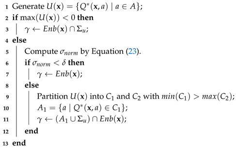
5. Case Studies for Quantitative Evaluations

The proposed approach is verified by two case studies related to industrial automation. To show the strengths of the new method on computational efficiency and control freedom, we compare it with two existing methods. Denoted as SCT + RL, method 1 combines SCT and RL and the RL controller chooses at most two controllable events at every reachable state [19]. The comparison shows that the new method requires similar learning time for RL but the K-means method significantly increases control freedom. Denoted as SCT, method 2 is the standard supervisory control synthesis method based on exhaustive search of finite state automata [30]. Method 2 ensures the supremal nonblocking supervisor. The comparison shows that the new approach can achieve a close-to-supremal supervisor.

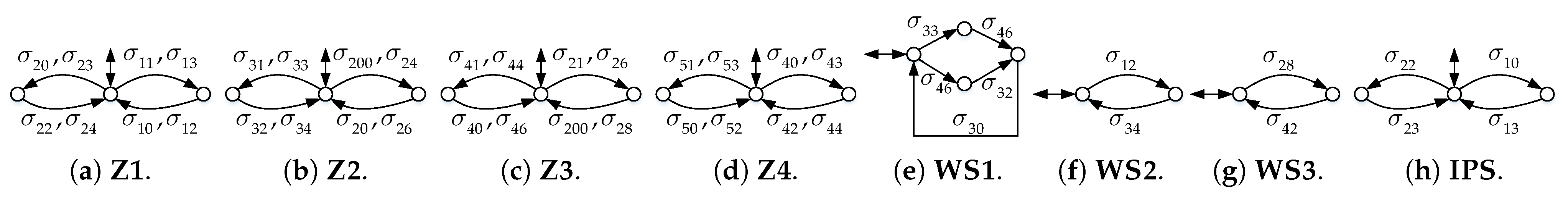
5.1. Supervisory Control of a Production Transfer Line

The first case study considers a production transfer line composed of two machines, ${\mathbf{M}}_1$ and ${\mathbf{M}}_2$, a testing unit $\mathbf{TU}$, and two intermediate product buffers, ${\mathbf{B}}_1$ and ${\mathbf{B}}_2$, as illustrated in Figure 2. Suppose that buffers ${\mathbf{B}}_1$ and ${\mathbf{B}}_2$ have storage capacities of 4 and 2, respectively.

In this system, machine ${\mathbf{M}}_1$ loads and processes a part, then transfers the completed part to buffer ${\mathbf{B}}_1$. Next, machine ${\mathbf{M}}_2$ retrieves a part from ${\mathbf{B}}_1$, processes it, and passes the finished item to buffer ${\mathbf{B}}_2$. The test unit $\mathbf{TU}$ picks up parts from ${\mathbf{B}}_2$ for inspection. If a part passes the quality test, it is discharged from the production line; otherwise, it is redirected back to ${\mathbf{B}}_1$ for reprocessing by ${\mathbf{M}}_2$. This operation introduces a feedback loop in the material flow. The system has two control requirements. (1) Buffers ${\mathbf{B}}_1$ and ${\mathbf{B}}_2$ must be protected against underflow and overflow. (2) The controlled system must not have any deadlock state.

The models of ${\mathbf{M}}_1,{\mathbf{M}}_2,\mathbf{TU},{\mathbf{B}}_1$, and ${\mathbf{B}}_2$ are displayed in Figure 3. The event sets of controllable and uncontrollable events are ${\Sigma }_c=\{{\mathit{ld}}_1,{\mathit{ld}}_2,\mathit{tst}\}$ and ${\Sigma }_u=\{{\mathit{uld}}_1,{\mathit{uld}}_2,\mathit{fns},\mathit{rjt}\}$, respectively. The models of the two buffers are specifications, and others are plant components. The proposed method first computes two reduced local modular supervisors, ${\mathbf{S}}_1$ and ${\mathbf{S}}_2$, based on the plant components and specifications, where ${\mathbf{S}}_1$ corresponds to ${\mathbf{B}}_1$ with nine states and 51 transitions, and ${\mathbf{S}}_2$ corresponds to ${\mathbf{B}}_2$ with three states and 12 transitions. With the restriction of ${\mathbf{S}}_1$ and ${\mathbf{S}}_2$, the controlled system satisfies the specification but leads to deadlocks.

For the new method, the initial global state is ${\mathbf{x}}_0=(q_{1,0},q_{2,0},q_{3,0},y_{1,0},y_{2,0})$, where $q_{1,0},q_{2,0},q_{3,0},y_{1,0}$ and $y_{2,0}$ are the initial states of ${\mathbf{M}}_1,{\mathbf{M}}_2,\mathbf{TU},{\mathbf{S}}_1$, and ${\mathbf{S}}_2$, respectively. The corresponding MDP is constructed as introduced in Section 4.1, where the action space is $\{{\mathit{ld}}_1,{\mathit{ld}}_2,\mathit{tst}\}$.

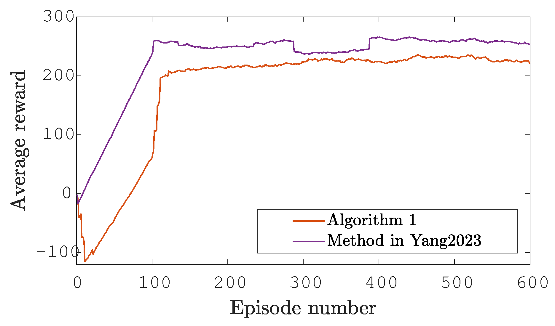
5.1.1. Computation of the Q Function Values

Algorithm 1 is applied to compute the optimal Q function, with the hyperparameters summarized in the first line in

Table 1. Values of parameters.

Parameter	$\mathit{\alpha }$	$\mathit{\lambda }$	$\mathit{ϵ}$	${\mathit{w}}_1$	${\mathit{w}}_2$	e	dec	MaxSt	MaxEp	Len
TL	0.9	0.96	0.98	30	−50	0.001	0.05	100	1000	30
AGV	0.95	0.99	0.95	30	−50	0.001	5 × 10−5	100	5000	100

. For instance, the used positive and negative rewards are $w_1=30$ and $w_2=-50$, respectively. Figure 4 shows the plots of average rewards for the past 30 episodes of the learning processes through Algorithm 1 and the SCT + RL method in our previous work [19]. In the SCT + RL method, the RL algorithm allows at most two controllable events at every reachable state. It shows that Algorithm 1 requires 300 episodes to converge but the SCT + RL method needs more than 400 episodes. The reason for this is that the action space sizes are three and four, respectively. Consequently, Algorithm 1 has a higher training efficiency.

5.1.2. Online Inference for the Final Supervisor

After training, the Q table stores the learned values for the pairs of reachable states and controllable events are obtained.

Table 2. Values of controllable events at four reachable states.

State	Controllable Events
	ld1	ld2	tst
${\mathbf{x}}_0$: (0,0,0,0,0)	68.77	−50	−50
${\mathbf{x}}_1$: (0,0,1,5,0)	89.41	51.41	83.66
${\mathbf{x}}_2$: (0,0,0,4,2)	82.89	−50	40.83
${\mathbf{x}}_3$: (1,1,0,6,1)	−42.88	−43.08	−43.29

displays the learned Q values at four reachable states. Each global state contains the state of five components: ${\mathbf{M}}_1,{\mathbf{M}}_2,\mathbf{TU},{\mathbf{S}}_1$, and ${\mathbf{S}}_2$, respectively.

Algorithm 2 is employed to decide the allowed events based on the learned Q function. For instance, as shown in Table 2, all values of controllable events at ${\mathbf{x}}_3$ are negative; hence, no controllable event is allowed at this state. Since the defined uncontrolled events are ${\mathit{uld}}_1$ and ${\mathit{uld}}_2$, the final permitted event subset at ${\mathbf{x}}_3$ is $\{{\mathit{uld}}_1,{\mathit{uld}}_2\}$. Moreover, controllable events are divided into $\{{\mathit{ld}}_1,\mathit{tst}\}$ and $\left\{{\mathit{ld}}_2\right\}$ at ${\mathbf{x}}_2$ according to the values, and the permitted event subset for ${\mathbf{x}}_2$ is $\{{\mathit{ld}}_1,\mathit{tst}\}$. Similarly, the determined event subset at ${\mathbf{x}}_0$ is $\left\{{\mathit{ld}}_1\right\}$. Since all values for controllable events at ${\mathbf{x}}_1$ are positive, Algorithm 2 computes ${\sigma }_{norm}=0.77$. If $\delta =0.5$, i.e., ${\sigma }_{norm}>\delta$, the controllable events are partitioned into $\{{\mathit{ld}}_1,\mathit{tst}\}$ and $\left\{{\mathit{ld}}_2\right\}$, and the decided controllable event subset is $\{{\mathit{ld}}_1,\mathit{tst}\}$. Since $\mathit{tst}$ is not allowed by the modular supervisors, the final permitted controllable event subset is $\left\{{\mathit{ld}}_1\right\}$. If $\delta =0.8$, all controllable events are selected, and the final permitted controllable event subset is $\{{\mathit{ld}}_1,{\mathit{ld}}_2\}$.

Figure 5 illustrates the relationship between the threshold parameter $\delta$ and the number of reachable states of the controlled system, where the number of nonblocking reachable states is 72 with $0.85\le \delta \le 0.88$. The result shows that the controlled system is blocking if $\delta >0.88$.

In this case, we employ $\delta =0.88$.

Table 3. Comparison of the control results by three methods.

Methods	SCT + RL	SCT + RL + K-Means	SCT
State space size	56	72	72
Nonblocking	Yes	Yes	Yes

presents the control results from three methods: integrating RL and SCT [19]; our new method combining RL, SCT, and K-means clustering; and directly employing SCT [31]. The results show that the SCT + RL method obtains a nonblocking supervisor of 56 reachable states. The novel SCT + RL + K-means method results in a nonblocking controlled system with 72 reachable states. For comparison, SCT is utilized to synthesize the supremal nonblocking supervisor, and the controlled system under this supervisor also achieves 72 reachable states. All three methods above obtain nonblocking supervisors. Our proposed method computes a nonblocking supervisor with equal number of reachable states as the supremal nonblocking supervisor does.

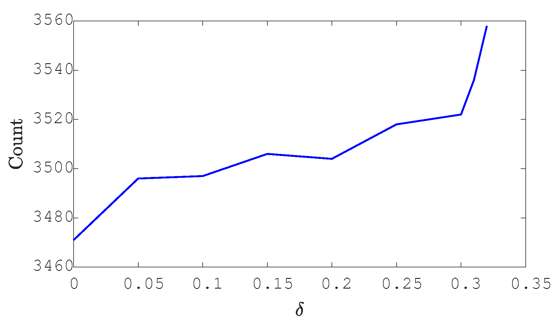
5.2. Control of an Automatically Guided Vehicles System

The second application is the control of automatically guided vehicles (AGVs) [19] for a manufacturing workcell. The system consists of 15 components, including two input stations (IPS1, IPS2), three workstations (WS1, WS2, WS3), five AGVs (AGV1–AGV5), four zones (Zone1–Zone4), and the station (CPS) for completed parts.

As shown in Figure 6, five AGVs travel on fixed circular routes, transporting parts to their designated places. Figure 7 and Figure 8 respectively display the DFA models of AGVs and specifications, where the controllable event set is

$${\Sigma }_c=\{{\sigma }_{11},{\sigma }_{13},{\sigma }_{21},{\sigma }_{23},{\sigma }_{31},{\sigma }_{33},{\sigma }_{41},{\sigma }_{43},{\sigma }_{51},{\sigma }_{53}\}$$

The models of the local modular supervisors corresponding to the specifications and the physical meanings of these events are illustrated in [19]. As a result, the controlled system under these modular supervisors has deadlocks.

A global state consists of the states of the five AGV models and the eight reduced modular supervisors by SCT. The constructed action set is $A={\Sigma }_c$, with 10 actions. The proposed method then applies Algorithm 1 to learn the value function $Q^{*}(\mathbf{x},a)$ for the MDP that corresponds to the global state transition system. Figure 9 shows the plots of average rewards for the past 100 episodes of the learning processes through Algorithm 1 and the proposed method in our previous work [19], where the parameters used are displayed in the “AGV case value” line in Table 1. Consequently, Algorithm 1 requires less than 3000 episodes, while the other needs more than 4000 episodes to get converged.

Algorithm 2 is then applied to infer the supervisor’s policy online. Figure 10 displays the variation of nonblocking reachable states with $\delta$. The largest number of states, 3558, is obtained when $\delta =0.32$, and the controlled system reaches deadlock if $\delta >0.32$. Therefore, we use $\delta =0.32$ in this case.

Table 4. Comparison of the control results by three methods.

Methods	SCT + RL	SCT + RL + K-Means	SCT
State space size	481	3558	4406
Nonblocking	Yes	Yes	Yes

presents the control results of the system under the method employed in the previous case. As a result, the controlled system with the SCT + RL method is nonblocking and includes 481 states, where the number of controllable events at a state is limited to, at most, two. Through the proposed method, the controlled system remains nonblocking and expands to 3558 states. Furthermore, With the supervisor by SCT, the controlled system achieves 4406 nonblocking reachable states. Compared with the method that only combines RL algorithms and SCT, the proposed method admits a much larger state size of the controlled system. Simultaneously, the satisfaction of the specifications is ensured.

6. Conclusions

This paper presents an integrated approach for nonblocking modular supervisory control in DESs by combining SCT, RL, and K-means clustering. The proposed method enhances learning efficiency by reducing the action space of RL algorithms while improving system freedom in RL-based supervisors. Through RL, the system efficiently learns values for all state action pairs, and K-means clustering infers the allowed controllable events online to ensure a balance between permissiveness and system constraints. Experimental validation on two case studies confirms the effectiveness of the new approach, demonstrating a significant increase in the number of nonblocking reachable states compared to prior methods.

In the future, we plan to enhance the scalability and adaptability of the approach by incorporating a Deep Q-Network (DQN). DQNs extends traditional Q-learning by using deep neural networks to approximate Q-values, enabling efficient learning in high-dimensional and large-scale discrete event systems. This will allow the system to handle more complex plant structures, larger event spaces, and dynamic environments without requiring exhaustive state enumeration. Furthermore, techniques such as experience replay and target networks [32] will be explored to stabilize training and improve convergence. Moreover, partial observability due to sensor noise, delays, or failures is one of our future works.

References

1. Wonham, W.M.; Cai, K. Supervisory Control of Discrete-Event Systems; Springer: Berlin/Heidelberg, Germany, 2019. [Google Scholar]
2. Patrik, B.; Fabian, M. Calculating Restart States for Systems Modeled by Operations Using Supervisory Control Theory. Machines 2013, 1, 116–141. [Google Scholar] [CrossRef]
3. Wonham, W.M.; Ramadge, P.J. Modular supervisory control of discrete-event systems. Math. Control. Signals Syst. 1988, 1, 13–30. [Google Scholar] [CrossRef]
4. Queiroz, M.H.d.; Cury, J.E.R. Modular supervisory control of large scale discrete event systems. In Proceedings of the International Conference on Discrete Event Systems, Anchorage, AK, USA, 27 September 2000; pp. 103–110. [Google Scholar]
5. Feng, L.; Wonham, W.M. Computationally Efficient Supervisor Design: Control Flow Decomposition. In Proceedings of the IEEE 8th International Workshop on Discrete Event Systems, Ann Arbor, MI, USA, 10–12 July 2006; pp. 9–14. [Google Scholar]
6. Goorden, M.; van de Mortel-Fronczak, J.; Reniers, M.; Fabian, M.; Fokkink, W.; Rooda, J. Model properties for efficient synthesis of nonblocking modular supervisors. Control Eng. Pract. 2021, 112, 104830. [Google Scholar] [CrossRef]
7. Schmidt, K.; Marchand, H.; Gaudin, B. Modular and decentralized supervisory control of concurrent discrete event systems using reduced system models. In Proceedings of the IEEE 8th International Workshop on Discrete Event Systems, Ann Arbor, MI, USA, 10–12 July 2006; pp. 149–154. [Google Scholar]
8. Schmidt, K.; Moor, T.; Perk, S. Nonblocking hierarchical control of decentralized discrete event systems. IEEE Trans. Autom. Control 2008, 53, 2252–2265. [Google Scholar] [CrossRef]
9. Leduc, R.J.; Brandin, B.A.; Lawford, M.; Wonham, W.M. Hierarchical interface-based supervisory control-part I: Serial case. IEEE Trans. Autom. Control 2005, 50, 1322–1335. [Google Scholar]
10. Liu, Y.; Liu, F. Optimal control of discrete event systems under uncertain environment based on supervisory control theory and reinforcement learning. Sci. Rep. 2024, 14, 25077. [Google Scholar] [CrossRef]
11. Dai, J.; Lin, H. A learning-based synthesis approach to decentralized supervisory control of discrete event systems with unknown plants. Control Theory Technol. 2014, 12, 218–233. [Google Scholar] [CrossRef]
12. Malik, R.; Åkesson, K.; Flordal, H.; Fabian, M. Supremica–an efficient tool for large-scale discrete event systems. IFAC-PapersOnLine 2017, 50, 5794–5799. [Google Scholar] [CrossRef]
13. Farooqui, A.; Hagebring, F.; Fabian, M. MIDES: A tool for supervisor synthesis via active learning. In Proceedings of the IEEE 17th International Conference on Automation Science and Engineering, Lyon, France, 23–27 August 2021; pp. 792–797. [Google Scholar]
14. Sutton, R.S.; Barto, A.G. Reinforcement Learning: An Introduction; MIT Press: Cambridge, MA, USA, 2018. [Google Scholar]
15. Kajiwara, K.; Yamasaki, T. Adaptive supervisory control based on a preference of agents for decentralized discrete event systems. In Proceedings of the IEEE SICE Annual Conference, Taipei, Taiwan, 18–21 August 2010; pp. 1027–1032. [Google Scholar]
16. Zielinski, K.M.C.; Hendges, L.V.; Florindo, J.B.; Lopes, Y.K.; Ribeiro, R.; Teixeira, M.; Casanova, D. Flexible control of Discrete Event Systems using environment simulation and Reinforcement Learning. Appl. Soft Comput. 2021, 111, 107714. [Google Scholar] [CrossRef]
17. Hu, Y.; Wang, D.; Yang, M.; He, J. Integrating reinforcement learning and supervisory control theory for optimal directed control of discrete-event systems. Neurocomputing 2024, 613, 128720. [Google Scholar] [CrossRef]
18. Konishi, M.; Sasaki, T.; Cai, K. Efficient safe control via deep reinforcement learning and supervisory control-csae study on multi-robot warehouse automation. IFAC-PapersOnLine 2022, 55, 16–21. [Google Scholar] [CrossRef]
19. Yang, J.; Tan, K.; Feng, L.; Li, Z. A model-based deep reinforcement learning approach to the nonblocking coordination of modular supervisors of discrete event systems. Inf. Sci. 2023, 630, 305–321. [Google Scholar] [CrossRef]
20. Yang, J.; Tan, K.; Feng, L.; El-Sherbeeny, A.M.; Li, Z. Reducing the learning time of reinforcement learning for the supervisory control of discrete event systems. IEEE Access 2023, 11, 59840–59853. [Google Scholar] [CrossRef]
21. Ran, X.; Xi, Y.; Lu, Y.; Wang, X.; Lu, Z. Comprehensive survey on hierarchical clustering algorithms and the recent developments. Artif. Intell. Rev. 2023, 56, 8219–8264. [Google Scholar] [CrossRef]
22. Kurani, A.; Doshi, P.; Vakharia, A.; Shah, M. A comprehensive comparative study of artificial neural network (ANN) and support vector machines (SVM) on stock forecasting. Ann. Data Sci. 2023, 10, 183–208. [Google Scholar] [CrossRef]
23. Kriegel, H.P.; Kröger, P.; Sander, J.; Zimek, A. Density-based clustering. Wiley Interdiscip. Rev. Data Min. Knowl. Discov. 2011, 1, 231–240. [Google Scholar] [CrossRef]
24. Bezdek, J.C.; Ehrlich, R.; Full, W. FCM: The fuzzy c-means clustering algorithm. Comput. Geosci. 1984, 10, 191–203. [Google Scholar] [CrossRef]
25. Ikotun, A.M.; Ezugwu, A.E.; Abualigah, L.; Abuhaija, B.; Heming, J. K-means clustering algorithms: A comprehensive review, variants analysis, and advances in the era of big data. Inf. Sci. 2023, 622, 178–210. [Google Scholar] [CrossRef]
26. Feng, L.; Wonham, W.M. TCT: A computation tool for supervisory control synthesis. In Proceedings of the IEEE 8th International Workshop on Discrete Event Systems, Ann Arbor, MI, USA, 10–12 July 2006; pp. 3–8. [Google Scholar]
27. Su, R.; Wonham, W.M. What information really matters in supervisor reduction? Automatica 2018, 95, 368–377. [Google Scholar] [CrossRef]
28. Malik, R.; Teixeira, M. Optimal modular control of discrete event systems with distinguishers and approximations. Discret. Event Dyn. Syst. 2021, 31, 659–691. [Google Scholar] [CrossRef]
29. Lewis, F.L.; Vrabie, D.; Vamvoudakis, K.G. Reinforcement learning and feedback control: Using natural decision methods to design optimal adaptive controller. IEEE Control Syst. Mag. 2012, 32, 76–105. [Google Scholar]
30. Feng, L.; Cai, K.; Wonham, W. A structural approach to the non-blocking supervisory control of discrete-event systems. Int. J. Adv. Manuf. Technol. 2009, 41, 1152–1168. [Google Scholar] [CrossRef]
31. Wonham, W.M.; Ramadge, P.J. On the supremal controllable sublanguage of a given language. SIAM J. Control Optim. 1987, 25, 637–659. [Google Scholar] [CrossRef]
32. Saglam, B.; Mutlu, F.B.; Cicek, D.C.; Kozat, S.S. Actor prioritized experience replay. J. Artif. Intell. Res. 2023, 78, 639–672. [Google Scholar] [CrossRef]
Figure 1. Schema for the proposed approach.
Machines 13 00559 g001
Figure 2. Illustration of the transfer line.
Machines 13 00559 g002
Figure 3. Component DES.
Machines 13 00559 g003
Figure 4. Plots of average rewards [19].
Machines 13 00559 g004
Figure 5. Variation of nonblocking reachable states with δ .
Machines 13 00559 g005
Figure 6. A manufacturing workcell with AGVs.
Machines 13 00559 g006
Figure 7. DFA models of AGVs.
Machines 13 00559 g007
Figure 8. DFA models of specifications on AGVs.
Machines 13 00559 g008
Figure 9. Plots of average rewards [19].
Machines 13 00559 g009
Figure 10. Variation of nonblocking reachable states with δ .
Machines 13 00559 g010