Clustered Correlation Health Scan Anomaly Detection Algorithm Applied for Fault Diagnosis in the Cylinders of a Marine Dual-Fuel Engine

Abstract

A novel anomaly detection algorithm is presented to analyze a group of signals that must be correlated under normal conditions. The method is called Clustered Correlation Health Scan (CCH-Scan). It detects abnormal signals, the durations corresponding to abnormalities, and the degree of abnormality. This algorithm is applied to a case study on fault diagnosis in the cylinders of a 12-cylinder marine dual-fuel engine. In particular, 12 Exhaust Valve Closing Dead Time (ECDT) signals are analyzed to detect abnormalities. Although these signals are critical and any abnormality in them requires urgent intervention, this is the first time they have been discussed in the literature. The details of the algorithm are elaborated, its parameters are studied, and the effects of these parameters on the results are measured and analyzed using a quality score. In addition, a metric to measure the degree of abnormality of the signal is introduced. The method detects abnormal signals, the durations of abnormalities, and the degrees of abnormalities. The results align with ground-truth data from an available technical industrial maintenance report. The approach demonstrates promising potential for application in various other contexts.

1. Introduction

Fault diagnosis is crucial in ensuring the reliability and safety of complex systems in various domains [1]. It involves identifying and addressing malfunctions that affect system performance, safety, and longevity. Fault diagnosis is important in many domains, such as aerospace, automotive, industrial manufacturing, healthcare, and marine systems. In particular, in marine systems, the harsh and unpredictable operational environment makes timely and precise fault diagnosis essential for maintaining vessel safety, optimizing performance, and reducing downtime.

Fault diagnosis methods can be classified into model-based and data-driven approaches [2]. Each approach has unique methodologies, advantages, and challenges, making them suitable for different scenarios depending on the availability of data and the nature of the system being analyzed. Model-based diagnosis employs analytical models derived from the physical processes of a system. It generates residuals by comparing measured and estimated variables, providing insights into the system’s dynamic behavior and enhancing the understanding of its physical operations. However, this approach faces challenges related to uncertainties caused by modeling errors and measurement inaccuracies. Despite these challenges, model-based diagnosis is suitable for scenarios with limited data availability. Data-driven diagnosis uses data monitoring for fault detection and classification. This approach employs techniques such as neural networks, Bayesian networks, and Principal Component Analysis, making it particularly effective for real-time processing due to its lower computational demands. However, it necessitates data processing and the extraction of relevant features from the data. Data-driven diagnosis is highly effective when a sufficient amount of data for both normal and faulty conditions is available. The approach introduced in this study can be classified as a data-driven anomaly detection method since it identifies abnormalities based solely on the analysis of signal data.

In fault diagnosis, it is essential to distinguish between faults and signal abnormalities. A fault is a defect or malfunction in a system component that results in improper operation or failure to meet performance criteria, typically associated with specific components or subsystems [3]. In contrast, signal abnormalities represent deviations from normal behavior, which may indicate faults, environmental changes, aging, or transient disturbances. While abnormalities reflect deviations from expected system performance, they do not always correspond to specific faults. When a pattern of abnormalities is observed consistently, particularly when related to key components or subsystems, it often suggests the presence of underlying faults.

Researchers have extensively utilized correlation and clustering techniques for fault diagnosis across various domains, including nuclear power plants, battery systems, and industrial processes. These methods often combine correlation analysis with clustering algorithms such as DBSCAN, K-means, and hierarchical clustering to enhance detection accuracy and feature relevance. However, most existing approaches are application-specific and lack generalizability, detailed anomaly characterization, and intuitive visualization capabilities, which limits their broader utility.

A novel anomaly detection algorithm is introduced, based on applying a clustering algorithm to the correlation matrix calculated from a set of signals during a specific, small time interval and repeating this process over the period of study. The algorithm is called Clustered Correlation Health Scan and is abbreviated as CCH-Scan. It is applied to a set of signals that must be correlated under normal conditions. CCH-Scan scans the signal over time and detects which signals show abnormal behavior and during which time intervals. An abnormal signal at a specific time period is a signal that behaves differently or is less correlated with the majority of the remaining signals.

The case study concerns fault diagnosis in the cylinders of a 12-cylinder dual-fuel marine engine, specifically the analysis of abnormalities in the ECDT signal using the CCH-Scan algorithm. The details of this signal will be explained later in the paper. Over a period of five months, 12 signals of the exhaust valve closing dead time (ECDT) were analyzed. ECDT is an important signal related to the closing of the exhaust valve in a marine dual-fuel engine, which will be described in Section 3. Abnormalities in such a signal usually require immediate intervention by engineers to perform an exhaust valve overhaul. The ECDT signal will be described in more detail later. The focus is to identify the cylinders with abnormal ECDT signals, the duration of ECDT signal abnormalities, and the degree of these abnormalities. The parameters of the algorithm will be examined, and their impact will be assessed using a quality score. A metric to evaluate the degree of abnormality in the signals will also be introduced. This approach effectively identifies abnormal signals, pinpoints the timing of abnormalities, and assesses the extent of these abnormalities. The findings are consistent with ground-truth data from a technical maintenance report, indicating strong potential for application in other contexts.

In summary, the primary contribution of this paper is the introduction of a novel Clustered Correlation Health Scan anomaly detection algorithm, applied to diagnosing cylinder faults in a marine dual-fuel engine. Specifically, this research addresses the issue of abnormal ECDT faults, which have not been extensively studied in the existing literature. Experimental validation was conducted to demonstrate the efficacy and reliability of the proposed algorithm.

The remainder of this paper is organized as follows: Section 2 presents related work in the literature. Section 3 introduces the exhaust system in a marine dual-fuel engine. Section 4 provides a detailed description of the CCH-Scan algorithm. In Section 5, faults identified in a technical report are discussed. Section 6 presents data cleaning, characteristics, and visualization. Section 7 discusses the results of applying the algorithm. Finally, Section 8 concludes the paper.

2. Related Work

Researchers have used correlation in different ways in their fault diagnosis methods across a wide variety of applications. Peng et al. proposed an intelligent fault diagnosis method for nuclear power plants (NPPs), based on correlation analysis (CA) for filtering irrelevant features and a Deep Belief Network (DBN) for fault detection through unsupervised pre-training and supervised fine-tuning, detecting multiple fault types using a dataset from a simulation model [4]. Liu et al. proposed a novel fault diagnosis algorithm, Correlation Coefficient-DBSCAN (CCDBSCAN), for power transformers based on Dissolved Gas Analysis (DGA) [5]. This method enhances traditional DBSCAN clustering by introducing a correlation coefficient to capture and amplify the similarity between transformer faults, thereby improving clustering accuracy. Cheng et al. introduced a spatio-temporal multi-correlation fusion (STMF) technique that integrates vibration signals from multiple sensors by exploring spatial correlations and applying adaptive weights. This method significantly enhances rotor bearing and gear failure diagnosis in rotor systems. By utilizing correlation analysis to fuse data from different sensors, the authors achieved notable improvements in diagnostic performance compared to other fusion methods [6]. He et al. introduced a Multiblock Temporal Convolutional Network (MBTCN) for fault diagnosis in multivariate processes, with a methodology that involves dividing variables into sub-blocks based on process mechanisms and utilizing a one-dimensional Temporal Convolutional Network to extract temporally correlated features within each sub-block [7]. Wang et al. proposed an advanced fault diagnosis method for lithium-ion battery systems using a multivariate statistical analysis-based cross-voltage correlation approach [8]. Their methodology combines Independent Component Analysis (ICA) and Principal Component Analysis (PCA) to process high-dimensional, non-Gaussian correlation coefficient (CC) signals efficiently.

Clustering algorithms such as DBSCAN, K-means, agglomerative, and mean shift clustering are widely adopted in various contexts and applications in fault detection and diagnosis systems. Li et al. proposed a method for diagnosing thermal runaway in EV lithium-ion batteries using DBSCAN clustering on voltage data [9]. Li et al. introduced a fault diagnosis method for rolling bearings that integrates symmetrized dot pattern (SDP) analysis with an improved density-based spatial clustering algorithm (ASDP-DBSCAN) [10]. SDP visualizes vibration signals for better pattern recognition, while optimized parameters and enhanced DBSCAN clustering improve accuracy and noise reduction. Wang et al. proposed FKM-ICS, an enhanced K-means clustering method for unbalanced vehicle fault diagnosis in railways [11]. It improves traditional K-means by using a novel cluster-center approximation and refined feature weights, leading to more accurate and efficient diagnostics. Yu et al. introduced a fault detection system using agglomerative hierarchical clustering combined with a stacked denoising autoencoder (SDAE) [12]. Fong et al. introduced a new fault diagnosis method using non-stationary vibration signals. They combined mean shift clustering with short-time Fourier transform to de-noise and extract time-varying harmonics without prior system knowledge [13].

Researchers have developed many anomaly detection methods that incorporate both correlation and clustering. These methods have been widely used in fault detection. Fields of application include mechanical systems, wireless sensor networks, and industrial processes.

Chen et al. proposed a method introducing K-medoids clustering to a three-direction correlation dimension to monitor the health state of wheel bearings [14]. The correlation dimension is a measure of the dimensionality of the space occupied by a set of random points. The algorithm begins by extracting 3D correlation dimensions from vibration signals in the x, y, and z directions, capturing the nonlinear dynamics of the bearings. These dimensions are then clustered using the K-medoids algorithm to group data into three states: normal, outer-ring fault, and cage fault. To address overlapping clusters, a two-step clustering refinement is applied, where subsets of data are clustered multiple times, and the resulting centers are re-clustered to create distinct, non-overlapping 3D spheres. These spheres represent the bearing states and are used for fault diagnosis by checking whether new vibration data falls within a specific sphere.

Yoo introduced a fault detection algorithm that utilizes sensor correlations to both reduce complexity and retain the physical interpretability of the data [15]. The process begins by normalizing sensor measurements collected during normal operations and calculating a correlation matrix across all sensor pairs. Only pairs with strong linear relationships are selected, and the corresponding two-dimensional data subsets are used to build clustering models—typically using Gaussian mixtures—to characterize normal operating behavior. When new data is received, it is normalized similarly and evaluated by computing the Mahalanobis distance from the established clusters. These distances are aggregated into a fault index that, if exceeding a set threshold, signals an anomaly.

Liu et al. introduced a Metric-Correlation-Based Fault Detection (MCFD) approach, a novel method to identify potential faults in wireless sensor networks that may evade detection by traditional spatiotemporal correlation techniques [16]. MCFD leverages internal system metric correlations within individual nodes. For each sensor, pairwise correlations between system metrics are quantified using Spearman’s rank correlation coefficient and aggregated into periodic correlation value views. These views are then analyzed using an improved density-based clustering algorithm, which identifies outliers by adapting to varying local densities.

Wang et al. introduced an automated fault detection method for cloud systems by analyzing workload-metric correlations [17]. The method first applies online incremental clustering to dynamically identify user access patterns, adapting to fluctuating workloads. Using canonical correlation analysis, it models relationships between workload vectors and multilayer system metrics. Anomalies are flagged via EWMA control charts that detect abrupt deviations in correlation coefficients.

3. Marine Dual-Fuel Engine

The marine dual-fuel engine operates on both liquefied natural gas (LNG) and diesel fuel. The engine is crucial for maritime propulsion, being the primary energy source for marine vessels. However, its significant contribution to greenhouse gas emissions requires improvements to reduce its environmental impact [18]. A dual-fuel engine is more efficient, flexible, and environmentally safer than traditional diesel engines. The use of LNG reduces the emission of air pollutant gases such as carbon dioxide (CO₂) and sulfur oxides (SOx) [19]. Robust performance is essential for a ship’s reliable operation and maneuverability, ensuring safe navigation and operational efficiency [20].

The dual-fuel engine comprises the five main subsystems of a diesel engine (fuel injection, air intake, exhaust, cooling, lubricating systems) [21], in addition to the gas supply system. The fuel and gas injection systems control fuel and gas delivery to the engine’s cylinders; the cooling system prevents overheating through water and air cooling; the lubrication system reduces friction and cleans engine parts [22]; and the air intake and exhaust systems manage combustion air supply and emissions. Given its complexity and the harsh operational environment at sea, effective fault diagnosis is vital.

The data used in this paper were collected from a two-stroke dual-fuel engine. Two-stroke engines complete a cycle in one crankshaft revolution, making them more efficient than four-stroke engines [23].

An exhaust system in a vessel’s engine is critical in managing emissions and ensuring compliance with environmental regulations. An exhaust manifold collects exhaust gases from the engine’s cylinders using an exhaust valve and directs them toward the turbocharger. The exhaust valve controls the flow of exhaust gases, making it the main component of the exhaust system. The valve’s opening and closing operations are controlled by a spring, air, and oil system, based on the crankshaft’s position, indicating the engine’s cycle stages. Therefore, the exhaust valve’s operation is linked to the crankshaft angle.

Faults in the exhaust system are considered critical due to their effect on performance and efficiency. One common fault is exhaust valve leakage, which leads to increased exhaust temperatures and reduced power output. Hu et al. explored the use of acoustic emission signals as one of the methods to address this problem [24]. Another significant concern is air leakage in the exhaust valve, which can compromise engine efficiency. Witkowski et al. identified this type of fault using PCA clustering analysis combined with neural networks [25]. Additionally, insufficient airflow in the air system can occur, impacting engine performance. Tu et al. addressed this issue by utilizing Kernel Principal Component Analysis (KPCA) for feature extraction [26]. Faults in turbines and air filters, such as clogging, are also critical for engine operation.

Basurko et al. employed artificial neural networks for diagnosing these faults [27]. Furthermore, exhaust pipe blockage can severely impede gas flow, affecting overall engine efficiency. Zhong et al. implemented techniques like semi-supervised PCA for timely detection, though other options also exist [28]. Finally, exhaust gas leakage, resulting from various system failures, presents another challenge for diesel engines. Wang et al. diagnosed this fault using hybrid techniques that combine manifold learning and anomaly detection [29]. This review shows the complexity of diagnosing faults in the exhaust system and the variety of approaches available. Despite extensive research on fault diagnosis in exhaust systems, the specific fault addressed in this study has not been previously explored in the literature.

During the opening of the exhaust valve, when the crankshaft reaches a certain angle, a signal from the Engine Control System (ECS) triggers the “exhaust valve open” command. This allows servo oil to flow through a rail valve, activating the Exhaust Valve Actuator. The actuator enables oil to enter the system, pushing a piston upwards to open the exhaust valve. During the valve closing process, at a different angle, the Engine Control System sends a “close” signal to the rail valve. A spring lowers the Exhaust Valve Actuator, releasing oil from beneath the piston. The oil then returns to the system, closing the exhaust valve as it drains back through the return pipe. This opening and closing mechanism of the exhaust valve is shown in Figure 1. The exhaust valve closing dead time (ECDT) refers to the time between the closing command and the initial movement of the spindle. The valve’s closing dead time is typically longer than its opening dead time, as shown in Figure 2.

4. CCH-Scan Algorithm

4.1. Principle

The proposed algorithm, CCH-Scan, analyzes a group of signals that normally exhibit correlation. CCH-Scan identifies deviations in the behavior of these signals, indicating the time intervals during which abnormalities occur. An abnormal signal is defined as one that shows less correlation (i.e., different behavior) compared to the majority of the other signals. The form of data used in the algorithm is described in Section 4.2.

The algorithm consists of an inner algorithm operating within an outer algorithm. Figure 3 provides a high-level overview of the CCH-Scan framework, illustrating its key stages, which will be elaborated further in this section. The inner algorithm uses the correlation between the signals to perform clustering within a small sliding window time interval, denoted as $[t_p;t_p+T]$. The inner algorithm is summarized in Algorithm 1 and explained in detail in Section 4.3.

In the outer algorithm, the inner algorithm operates on a sliding window time interval $[t_p;t_p+T]$ with a duration of T, which slides with a time shift $s<T$ over the entire study period represented by the time interval $[t_1;t_R]$. The outer algorithm is summarized in Algorithm 2 and explained in detail in Section 4.4.

The outer algorithm is divided into two main steps: the application of the inner algorithm and the aggregation of results.

In the application step of the outer algorithm, it is assumed that $t_p=p\times s$, where p is an index referring to the sliding window time interval $[t_p;t_p+T]=[p\times s;p\times s+T]$.

In the aggregation step, the total study period $[t_1;t_R]$ is divided into smaller intervals $[q\times s;(q+1)\times s]$. For each interval $[q\times s;(q+1)\times s]$, the results obtained from all intervals $[p\times s;p\times s+T]$ are aggregated under the condition that $[q\times s;(q+1)\times s]\subseteq [p\times s;p\times s+T]$. The way in which the total period of study is divided is elaborated in Figure 4.

Algorithm 1 Inner Algorithm

1: Input: Signals ${\mathbf{X}}_{\mathbf{i}}\left({\mathbf{t}}_{\mathbf{p}}\right)$, Algorithm C  2: Calculate correlation matrix:  3: for each i,j in 1 to N do  4:     $c_{ij}\left(t_p\right)\leftarrow \rho ({\mathbf{X}}_{\mathbf{i}}\left({\mathbf{t}}_{\mathbf{p}}\right),{\mathbf{X}}_{\mathbf{j}}\left({\mathbf{t}}_{\mathbf{p}}\right))$  5: end for  6: Calculate discretized correlation matrix:  7: for each $i,j$ in 1 to N do  8:     if $|c_{ij}\left(t_p\right)|\ge x$ then  9:         $d_{ij}\left(t_p\right)\leftarrow 1$ 10:     else 11:         $d_{ij}\left(t_p\right)\leftarrow 0$ 12:     end if 13: end for 14: Cluster the discretized correlation matrix: 15: $Y_1\left(t_p\right),\dots Y_N\left(t_p\right)\leftarrow C\left(\mathbf{D}\left({\mathbf{t}}_{\mathbf{p}}\right)\right)$ 16: Determine the cluster with most signals: 17: $L\left(t_p\right)\leftarrow MODE\left(Y_i\left(t_p\right)\right)$ 18: for each i do 19:     Compute Abnormality Indicator: 20:     if $Y_i\left(t_p\right)\ne L\left(t_p\right)$ then 21:         $F_i\left(t_p\right)\leftarrow 1$ 22:         add ${\mathbf{D}}_{\mathbf{i}}\left({\mathbf{t}}_{\mathbf{p}}\right)$ to ${\mathcal{C}}_1\left(t_p\right)$ 23:     else 24:         $F_i\left(t_p\right)\leftarrow 0$ 25:         add ${\mathbf{D}}_{\mathbf{i}}\left({\mathbf{t}}_{\mathbf{p}}\right)$ to ${\mathcal{C}}_0\left(t_p\right)$ 26:     end if 27:     Compute Abnormality Metric:      $z_j\left(t_p\right)\leftarrow {\displaystyle \frac{{\sum }_{{\mathbf{D}}_{\mathbf{k}}\left({\mathbf{t}}_{\mathbf{p}}\right)\in {\mathcal{C}}_0\left(t_p\right)}{d}_{kj}\left(t_p\right)}{|{\mathcal{C}}_0\left(t_p\right)|}}$ 28:     $A_i\left(t_p\right)\leftarrow {\sum }_{j=1}^N\left|d_{ij}\left(t_p\right)-z_j\left(t_p\right)\right|$ 29: end for 30: Calculate Overall Silhouette Score $S\left(t_p\right)$: 31: for each $u,v$ in 1 to N do 32:     ${\delta }_{uv}\left(t_p\right)\leftarrow \sqrt{{\sum }_{j=1}^N{\left(d_{uj}\left(t_p\right)-d_{vj}\left(t_p\right)\right)}^2}$ 33: end for 34: for each u in 1 to N do 35:     $a_u\left(t_p\right)\leftarrow {\displaystyle \frac{1}{|{\mathcal{C}}_{F_u\left(t_p\right)}\left(t_p\right)|-1}}{\sum }_{{\mathbf{D}}_{\mathbf{j}}\left({\mathbf{t}}_{\mathbf{p}}\right)\in {\mathcal{C}}_{F_u\left(t_p\right)},v\ne u}{\delta }_{uv}\left(t_p\right)$ 36:     $b_u\left(t_p\right)\leftarrow {\displaystyle \frac{1}{|{\mathcal{C}}_{1-F_u\left(t_p\right)}\left(t_p\right)|}}{\sum }_{{\mathbf{D}}_{\mathbf{v}}\left({\mathbf{t}}_{\mathbf{p}}\right)\in {\mathcal{C}}_{1-F_u\left(t_p\right)}}{\delta }_{uv}\left(t_p\right)$ 37:     $s_u\left(t_p\right)\leftarrow {\displaystyle \frac{b_u\left(t_p\right)-a_u\left(t_p\right)}{max(a_u\left(t_p\right),b_u\left(t_p\right))}}$ 38: end for 39: $S\left(t_p\right)\leftarrow {\displaystyle \frac{1}{N}}{\sum }_{u=1}^N{s}_u\left(t_p\right)$ 40: Output:$F_i\left(t_p\right)$, $A_i\left(t_p\right)$, $S\left(t_p\right)$

Algorithm 2 CCH-Scan Algorithm

1: Input: $\mathbf{X}$, Algorithm C, x, s, T  2: $p,t_p\leftarrow 0$  3: while  $p\times s\le t_r$  do  4:     ${\mathbf{X}}_{\mathbf{i}}\left({\mathbf{t}}_{\mathbf{p}}\right)\leftarrow {[x_i\left(t_m\right),x_i\left(t_{m+1}\right),...,x_i\left(t_{m+l}\right)]}^T$ s.t.  5:     $t_p\le t_m<t_{m+1}<...<t_{m+l}\le t_p+T$  6:     $t_p,F_i\left(t_p\right),A_i\left(t_p\right),S\left(t_p\right)\leftarrow$ INNER(${\mathbf{X}}_{\mathbf{i}}\left({\mathbf{t}}_{\mathbf{p}}\right)$,C)  7:     SAVE ($t_p,F_i\left(t_p\right),A_i\left(t_p\right),S\left(t_p\right)$)  8:     $p\leftarrow p+1$  9:     $t_p\leftarrow p\times s$ 10: end while 11: $q,t_q\leftarrow 0$ 12: while  $q\times s\le t_r$  do 13:     $l,c,Qcount,Rcount\leftarrow 0$ 14:     while $c\times s\le t_r$ do 15:         if $c\times s\le t_q$ and $t_{q+1}\le c\times s+T$ then 16:            $l\leftarrow l+1$ 17:            $count\leftarrow count+1$ 18:            for each i in 1 to N do 19:                $F_{l,i}^{\prime },\leftarrow F_i\left(t_c\right)$ 20:                $A_{l,i}^{\prime }\leftarrow A_i\left(t_c\right)$ 21:            end for 22:            $S_l^{\prime }\leftarrow S\left(t_c\right)$ 23:            SAVE $l,\left(F_{l,i}^{\prime }\right),A_{l,i}^{\prime },S_l^{\prime }$ 24:            for each i in 1 to N do 25:                if $F_i\left(t_c\right)=1$ then 26:                    $Qcoun{t}_i\leftarrow Qcoun{t}_i+1$ 27:                else 28:                    $Rcoun{t}_i\leftarrow Rcoun{t}_i+1$ 29:                end if 30:            end for 31:         end if 32:         $c\leftarrow c+1$ 33:     end while 34:     for each i in 1 to N do 35:         $Q_i(q\times s)\leftarrow Qcoun{t}_i$ 36:         $R_i(q\times s)\leftarrow Rcoun{t}_i$ 37:         if $Q_i(q\times s)\ge R_i(q\times s)$ then 38:            $I_i(q\times s)\leftarrow 1$ 39:         else 40:            $I_i(q\times s)\leftarrow 0$ 41:         end if 42:         $V_i(q\times s)={\displaystyle \frac{Qcoun{t}_i}{Qcoun{t}_i+Rcoun{t}_i}}$ 43:     end for 44:     if $\exists i/I_i(q\times s)=1$ then 45:         $L(q\times s))\leftarrow 1$ 46:     else 47:         $L(q\times s))\leftarrow 0$ 48:     end if 49:     $S(q\times s)\leftarrow {\displaystyle \frac{{\sum }_l{S}_l^{\prime }}{Qcoun{t}_i+Rcoun{t}_i}}\times L(q\times s)$ 50:     for each i in 1 to N do 51:         $A_i(q\times s)\leftarrow {\displaystyle \frac{{\sum }_l{A}_{l,i}^{\prime }}{Qcoun{t}_i+Rcoun{t}_i}}\times L(q\times s)$ 52:     end for 53:     $q\leftarrow q+1$ 54:     $t_q\leftarrow q\times s$ 55: end while 56: Output: $I_i(q\times s)$, $F_i(q\times s)$, $A_i(q\times s)$, $S(q\times s)$

4.2. Data Definition

The data used by the algorithm is a group of signals. This data is represented in the form of a matrix $\mathbf{X}$ as shown in (1).

$$\mathbf{X}=\left[\begin{array}{ccc}{x}_1\left(t_1\right)& \dots & x_N\left(t_1\right)\\ x_1\left(t_2\right)& \dots & x_N\left(t_2\right)\\ ⋮& & ⋮\\ x_1\left(t_R\right)& \dots & x_N\left(t_R\right)\end{array}\right]$$

(1)

The rows of matrix $\mathbf{X}$ represent the signals, and the columns represent the time instances. The number of signals to be analyzed is N. Each signal ${\mathbf{X}}_{\mathbf{k}}$ has an index k, where $k\in 1,2,\dots ,N$.

${\mathbf{X}}_{\mathbf{k}}$ has R values, where each value is denoted as $x_k\left(t_i\right)$ and corresponds to a time instance $t_i$. ${\mathbf{X}}_{\mathbf{k}}$ can be represented as in (2).

$${\mathbf{X}}_{\mathbf{k}}={[x_k\left(t_1\right),\dots ,x_k\left(t_R\right)]}^T$$

(2)

The integer i is an index that refers to the order of the elements with respect to time. For simplicity, the reference of time starts at $t_1=0$. It is given that $t_1<\cdots <t_i<t_{i+1}<\cdots <t_R$.

4.3. Inner Algorithm

The inner algorithm applied on the interval $[t_p;t_p+T]$ is divided into six steps, where computations are performed.

• Computing the correlation matrix.
  The signal ${\mathbf{X}}_{\mathbf{i}}\left({\mathbf{t}}_{\mathbf{p}}\right)$ is a portion of the signal ${\mathbf{X}}_{\mathbf{i}}$ and is represented as shown in (3). It is given that $t_p\le t_m<t_{m+1}<...<t_{m+l}\le t_p+T$. The correlation matrix $\mathbf{C}\left({\mathbf{t}}_{\mathbf{p}}\right)$ shown in (4) has elements $c_{ij}\left(t_p\right)$. Each of the elements $c_{ij}\left(t_p\right)$ is the Pearson Correlation between the two signals ${\mathbf{X}}_{\mathbf{i}}\left({\mathbf{t}}_{\mathbf{p}}\right)$ and ${\mathbf{X}}_{\mathbf{j}}\left({\mathbf{t}}_{\mathbf{p}}\right)$ with $i,j\in \{1,2,...,N\}$ as shown in (5). The rows of the correlation matrix represent the signals, and the columns represent how much these signals correlate to the other signals. All the diagonal elements of the correlation matrix are equal to 1.

  $${\mathbf{X}}_{\mathbf{i}}\left({\mathbf{t}}_{\mathbf{p}}\right)={[x_i\left(t_m\right),x_i\left(t_{m+1}\right),...,x_i\left(t_{m+l}\right)]}^T$$

  (3)

  $$\mathbf{C}\left({\mathbf{t}}_{\mathbf{p}}\right)=\left[\begin{array}{ccc}{c}_{11}\left(t_p\right)& \dots & c_{1N}\left(t_p\right)\\ c_{21}\left(t_p\right)& \dots & c_{2N}\left(t_p\right)\\ ⋮& & ⋮\\ c_{N1}\left(t_p\right)& \dots & c_{NN}\left(t_p\right)\end{array}\right]$$

  (4)

  $$c_{ij}\left(t_p\right)=\rho ({\mathbf{X}}_{\mathbf{i}}\left({\mathbf{t}}_{\mathbf{p}}\right),{\mathbf{X}}_{\mathbf{j}}\left({\mathbf{t}}_{\mathbf{p}}\right))$$

  (5)
• Computing the discretized correlation matrix.
  The discretized correlation matrix $\mathbf{D}\left({\mathbf{t}}_{\mathbf{p}}\right)$ shown in (6) has elements $d_{ij}\left(t_p\right)$ shown in (7). The number $x\in [0,1]$ is a threshold representing the value above which, when the absolute value of the correlation exceeds, the correlation is considered sufficiently correlated. The choice of x will be discussed later. The value $d_{ij}\left(t_p\right)$ of the matrix $\mathbf{D}\left({\mathbf{t}}_{\mathbf{p}}\right)$ represents whether the correlation between the sub-signal ${\mathbf{X}}_{\mathbf{i}}\left({\mathbf{t}}_{\mathbf{p}}\right)$ and ${\mathbf{X}}_{\mathbf{j}}\left({\mathbf{t}}_{\mathbf{p}}\right)$ is considered sufficiently correlated or not. The aim is to group the signals based on the correlation with each of the other signals. The rows ${\mathbf{D}}_{\mathbf{i}}\left({\mathbf{t}}_{\mathbf{p}}\right)$ of the matrix $\mathbf{D}\left({\mathbf{t}}_{\mathbf{p}}\right)$ represent a signal ${\mathbf{X}}_{\mathbf{i}}\left({\mathbf{t}}_{\mathbf{p}}\right)$, and the columns of the matrix represent the evaluation of the correlation with the other signals.

  $$\mathbf{D}\left({\mathbf{t}}_{\mathbf{p}}\right)=\left[\begin{array}{ccc}{d}_{11}\left(t_p\right)& \dots & d_{1N}\left(t_p\right)\\ d_{21}\left(t_p\right)& \dots & d_{2N}\left(t_p\right)\\ ⋮& & ⋮\\ d_{N1}\left(t_p\right)& \dots & d_{NN}\left(t_p\right)\end{array}\right]$$

  (6)

  $$d_{ij}\left(t_p\right)=\left\{\begin{array}{cc}1\hfill & \mathrm{if}|c_{ij}\left(t_p\right)|\ge x\hfill \\ 0\hfill & \mathrm{if}|c_{ij}\left(t_p\right)|<x\hfill \end{array}\right.$$

  (7)
• Applying a clustering algorithm.
  The integer i can be seen as an index to the elements to be classified and j as an index to the features describing these elements. The signals to be classified are represented by the elements in the set $\mathcal{X}\left(t_p\right)$ as shown in (8). An element ${\mathbf{D}}_{\mathbf{i}}\left({\mathbf{t}}_{\mathbf{p}}\right)$, which corresponds to a signal, is a horizontal vector as shown in (9).

  $$\mathcal{X}\left(t_p\right)=\{{\mathbf{D}}_{\mathbf{1}}\left({\mathbf{t}}_{\mathbf{p}}\right),{\mathbf{D}}_{\mathbf{2}}\left({\mathbf{t}}_{\mathbf{p}}\right),...,{\mathbf{D}}_{\mathbf{i}}\left({\mathbf{t}}_{\mathbf{p}}\right)\}$$

  (8)

  $${\mathbf{D}}_{\mathbf{i}}\left({\mathbf{t}}_{\mathbf{p}}\right)=[d_{i1}\left(t_p\right),\dots ,d_{iN}\left(t_p\right)]$$

  (9)
  A clustering algorithm C such as DBSCAN, Meanshift, K-means, or any other algorithm is applied to the discretized correlation matrix $\mathbf{D}\left({\mathbf{t}}_{\mathbf{p}}\right)$. The result of the clustering is a cluster ${\mathbf{Y}}_{\mathbf{i}}\left({\mathbf{t}}_{\mathbf{p}}\right)$ for each $i\in \{1,2,...,N\}$. No specific clustering algorithm must be used, but some algorithms may show better results than others. Table 1 provides an overview of some widely used clustering algorithms and some of their parameters.

Table 1. Popular clustering algorithms.

Algorithm	Parameters	Concept
DBSCAN clustering [30].	- $ϵ$: Maximum distance for neighbors. - $\mathcal{N}$: Minimum neighbors for a core point	Groups points that are closely packed and labels points in low-density areas as outliers.
K-Means clustering [31].	- k: Number of clusters.	Partitions data into k clusters by minimizing squared distances between points and their nearest centroid.
agglomerative clustering [32].	- $\mathcal{N}$: desired number of clusters. - Distance metrics. - Linkage criteria.	A bottom-up approach where each point starts as its own cluster and merges based on distance between clusters.
Mean shift clustering [33].	- W: Bandwidth.	Locates dense regions in the data by shifting centroids to the mean of points within a defined radius.

Table 1. Popular clustering algorithms.

Algorithm	Parameters	Concept
DBSCAN clustering [30].	- $ϵ$: Maximum distance for neighbors. - $\mathcal{N}$: Minimum neighbors for a core point	Groups points that are closely packed and labels points in low-density areas as outliers.
K-Means clustering [31].	- k: Number of clusters.	Partitions data into k clusters by minimizing squared distances between points and their nearest centroid.
agglomerative clustering [32].	- $\mathcal{N}$: desired number of clusters. - Distance metrics. - Linkage criteria.	A bottom-up approach where each point starts as its own cluster and merges based on distance between clusters.
Mean shift clustering [33].	- W: Bandwidth.	Locates dense regions in the data by shifting centroids to the mean of points within a defined radius.

4.

Computing the Abnormality Indicator.

In the scenario of normal behavior and perfect conditions, the system is expected to operate where all the signals must be correlated. So, the largest number of signals should be in correlation with each other. If a few signals operate with less correlation with the majority, they are considered to perform abnormally. Based on this, it is assumed that the cluster with the largest number of signals is the normal cluster, and any other signal outside this cluster is abnormal. The abnormality indicator $F_i\left(t_p\right)$ indicates if a signal ${\mathbf{X}}_{\mathbf{i}}\left({\mathbf{t}}_{\mathbf{p}}\right)$ is considered abnormal by the inner algorithm during the sliding window time interval $[t_p;t_p+T]$. The computation of $F_i\left(t_p\right)$ is shown in (10), where $L\left(t_p\right)$ is the cluster that has the largest number of points.

Using the abnormality indicator $F_i\left(t_p\right)$, two clusters can be defined, the normal cluster ${\mathcal{C}}_0\left(t_p\right)$ and the abnormal cluster ${\mathcal{C}}_1\left(t_p\right)$, as shown in (11) and (12) respectively. The classified signals are either in the normal or the abnormal cluster, as shown in (13).

$$F_i\left(t_p\right)=\left\{\begin{array}{cc}0\hfill & \mathrm{if}{Y}_i\left(t_p\right)=L\left(t_p\right)\hfill \\ 1\hfill & \mathrm{if}else\hfill \end{array}\right.$$

(10)

$${\mathcal{C}}_0\left(t_p\right)=\{{\mathbf{D}}_{\mathbf{i}}\left({\mathbf{t}}_{\mathbf{p}}\right)\mid F_i\left(t_p\right)=0\}$$

(11)

$${\mathcal{C}}_1\left(t_p\right)=\{{\mathbf{D}}_{\mathbf{i}}\left({\mathbf{t}}_{\mathbf{p}}\right)\mid F_i\left(t_p\right)=1\}$$

(12)

$$\mathcal{X}\left(t_p\right)={\mathcal{C}}_0\left(t_p\right)\cup {\mathcal{C}}_1\left(t_p\right)$$

(13)

5.

Computing the Degree of Abnormality Metric.

The degree of abnormality metric $A_i\left(t_p\right)$ measures the extent of difference between a signal and normal signals. It is equal to the Manhattan distance between the i-th signal, represented by ${\mathbf{D}}_{\mathbf{i}}\left({\mathbf{t}}_{\mathbf{p}}\right)$ shown in (14), and the center of the normal cluster, represented by $z\left(t_p\right)$ shown in (15). The center of the normal cluster $z_j\left(t_p\right)$ is calculated as shown in (16), where $|{\mathcal{C}}_0\left(t_p\right)|$ is the number of normal signals. The formula to compute the degree of abnormality metric $A_i\left(t_p\right)$ is shown in (17).

$${\mathbf{D}}_{\mathbf{i}}\left({\mathbf{t}}_{\mathbf{p}}\right)=[d_{i1}\left(t_p\right)\dots d_{iN}\left(t_p\right)]$$

(14)

$$z\left(t_p\right)=[z_1\left(t_p\right)\dots z_N\left(t_p\right)]$$

(15)

$$z_j\left(t_p\right)={\displaystyle \frac{{\sum }_{D_k\left(t_p\right)\in {\mathcal{C}}_0\left(t_p\right)}{d}_{kj}\left(t_p\right)}{|{\mathcal{C}}_0\left(t_p\right)|}}$$

(16)

$$A_i\left(t_p\right)=\sum _{j=1}^N\left|d_{ij}\left(t_p\right)-z_j\left(t_p\right)\right|$$

(17)

6.

Calculating the overall Silhouette Score.

The overall Silhouette Score $S\left(t_p\right)$ measures the quality of clustering, with values close to 1 indicating well-separated clusters and values near −1 indicating potential misclassification of points [34]. In order to calculate the overall Silhouette Score $S\left(t_p\right)$, the Silhouette Score $s_u\left(t_p\right)$ for each signal of index u is calculated first based on the value of the abnormality indicator $F_u\left(t_p\right)$. The cluster ${\mathcal{C}}_{F_u\left(t_p\right)}\left(t_p\right)$ represents the cluster to which ${\mathbf{D}}_{\mathbf{u}}\left({\mathbf{t}}_{\mathbf{p}}\right)$ belongs, and ${\mathcal{C}}_{1-F_u\left(t_p\right)}\left(t_p\right)$ represents the opposite cluster. The computation of $s_u\left(t_p\right)$, shown in (21), is based on the computations shown in (18)–(20). Then, the average silhouette coefficient $S\left(t_p\right)$ across all signals is calculated as shown in (22).

$$a_u\left(t_p\right)={\displaystyle \frac{1}{|{\mathcal{C}}_{F_u\left(t_p\right)}\left(t_p\right)|-1}}\sum _{{\mathbf{D}}_{\mathbf{j}}\left({\mathbf{t}}_{\mathbf{p}}\right)\in {\mathcal{C}}_{F_u\left(t_p\right)},v\ne u}{\delta }_{uv}\left(t_p\right)$$

(18)

$$b_u\left(t_p\right)={\displaystyle \frac{1}{|{\mathcal{C}}_{1-F_u\left(t_p\right)}\left(t_p\right)|}}\sum _{{\mathbf{D}}_{\mathbf{v}}\left({\mathbf{t}}_{\mathbf{p}}\right)\in {\mathcal{C}}_{1-F_u\left(t_p\right)}}{\delta }_{uv}\left(t_p\right)$$

(19)

$${\delta }_{uv}\left(t_p\right)=\sqrt{\sum _{j=1}^N{\left(d_{uj}\left(t_p\right)-d_{vj}\left(t_p\right)\right)}^2}$$

(20)

$$s_u\left(t_p\right)={\displaystyle \frac{b_u\left(t_p\right)-a_u\left(t_p\right)}{max(a_u\left(t_p\right),b_u\left(t_p\right))}}$$

(21)

$$S\left(t_p\right)={\displaystyle \frac{1}{N}}\sum _{u=1}^N{s}_u\left(t_p\right)$$

(22)

4.4. Outer Algorithm

The outer algorithm is applied to the total period of study represented by the interval $[t_1=0;t_R]$. The outer algorithm is summarized in Algorithm 2, and it is composed of two steps. Step 1 is dedicated to applying the inner algorithms using a sliding window. Step 2 is dedicated to aggregating the results.

• Applying the inner algorithm.
  A window with an interval $[p\times s;p\times s+T]\in [t_1;t_R]$ is used. This window has a size T and slides with each iteration p by a duration of s until reaching the end of the interval $[t_1;t_R]$, as elaborated in Figure 4. It is assumed that $s<T$. For each iteration p, the algorithm is applied, and the result obtained is the abnormality indicators $F_i(p\times s)$, the Silhouette Score $S(p\times s)$, and the degree of abnormality metrics $A_i(p\times s)$.
• Aggregating the results.
  The interval $[t_1;t_R]$ is divided into sub-intervals $[q\times s;(q+1)\times s]$. In each iteration q, the following are computed:
  • The number of positive votes $Q_i(q\times s)$, which is the number of times the inner algorithm considered the signal of index i an abnormal signal.

    $$Q_i(q\times s)=\sum _{\begin{array}{c}[q\times s;(q+1)\times s]\subseteq [p\times s;p\times s+T]\\ F_i(p\times s)=1\end{array}}1$$

    (23)
  • The number of negative votes $R_i(q\times s)$, which is the number of times the inner algorithm considered the signal of index i a normal signal.

    $$R_i(q\times s)=\sum _{\begin{array}{c}[q\times s;(q+1)\times s]\subseteq [p\times s;p\times s+T]\\ F_i(p\times s)=0\end{array}}1$$

    (24)
  • The abnormality indicator $I_i(q\times s)$, which indicates whether the signal i on interval $[q\times s;(q+1)\times s]$ is considered abnormal or not.

    $$I_i(q\times s)=\left\{\begin{array}{cc}1\hfill & \mathrm{if}{Q}_i(q\times s)\ge R_i(q\times s)\hfill \\ 0\hfill & \mathrm{if}else\hfill \end{array}\right.$$

    (25)
  • The voting score $V_i(q\times s)$, which indicated how many times from the total number of decisions the inner algorithm considered the signal i abnormal.

    $$V_i(q\times s)={\displaystyle \frac{Q_i(q\times s)}{Q_i(q\times s)+R_i(q\times s)}}$$

    (26)
    The voting score measures how consistent the algorithm is in deciding the abnormality of a signal while changing the interval of study. It can be used to filter some results with a voting score less than a threshold.
  • The global abnormality indicator $L(q\times s)$ which indicates that if there is at least one abnormality in the whole set of N signals.

    $$L(q\times s)=\left\{\begin{array}{cc}1\hfill & \mathrm{if}\exists i/I_i(q\times s)=1\hfill \\ 0\hfill & \mathrm{if}else\hfill \end{array}\right.$$

    (27)
  • The abnormality clustering quality score (CQ) $S(q\times s)$ measures the quality of clustering of the algorithm for the interval $[q\times s;(q+1)\times s]$. It is only defined if $L(q\times s)=1$ and calculated as follows:

    $$S(q\times s)=\mathbb{E}\left[S\right(p\times s)\mid q\times s;(q+1)\times s]\times L(q\times s)$$

    (28)
  • The average degree of abnormality metric $A_i(q\times s)$ measures how much a signal is far from the normally behaving signal while considering the calculations by the inner algorithm.

    $$A_i(q\times s)=\mathbb{E}[A_i(p\times s)\mid q\times s;(q+1)\times s]$$

    (29)

4.5. Abnormalities Detection

An abnormality ${\mathcal{F}}_w$ obtained by the algorithm can be defined as:

$${\mathcal{F}}_w=(w,[s_w;e_w],{\mathcal{Z}}_w,{\mathcal{A}}_w,{\mathcal{S}}_w,{\mathcal{V}}_w)$$

(30)

The characteristics of the abnormality are obtained as follows:

• w is the abnormality number, an integer used to identify the abnormality.
• $s_w$ is the start time of the abnormality. It is the time $s_w=q\times s$ when the abnormality indicator $I_i$ changes from 0 to 1.
• $e_w$ is the end time of the abnormality. It is the time $e_w=q\times s$ when the abnormality indicator $I_i$ changes from 1 to 0.
• ${\mathcal{Z}}_w$ is the signal number i, which the abnormality corresponds to.
• ${\mathcal{A}}_w$ is the abnormality’s degree of abnormality.

  $${\mathcal{A}}_w=\sum _{t_q=s_w}^{e_w}{A}_i\left(t_q\right)$$

  (31)
• ${\mathcal{S}}_w$ is the algorithm’s quality score to obtain this abnormality.

  $${\mathcal{S}}_w=\sum _{t_q=s_w}^{e_w}S\left(t_q\right)$$

  (32)
• ${\mathcal{V}}_w$ is the algorithm’s voting score to obtain this abnormality.

$${\mathcal{V}}_w=\sum _{t_q=s_w}^{e_w}{V}_i\left(t_q\right)$$

(33)

The two scores ${\mathcal{S}}_w$ and ${\mathcal{V}}_w$ are used to measure the significance of obtaining the abnormality by the algorithm and can be used to filter some of the abnormalities. ${\mathcal{S}}_w$ shows the quality of the clustering that allowed obtaining this abnormality, while ${\mathcal{V}}_w$ measures the degree of consistency of the algorithm’s result within the calculations from multiple time intervals.

4.6. Algorithm Evaluation

The following two parameters are used to evaluate the algorithm:

• The total duration with abnormalities:

  $$D=\sum _{L(q\times s)=1}s$$

  (34)
• The clustering quality:

  $$Q={\displaystyle \frac{{\sum }_{L(q\times s)=1}S(q\times s)}{{\sum }_{L(q\times s)=1}1}}$$

  (35)

5. Faults and Abnormal ECDT Signals

The results from the algorithm are to be compared with abnormalities associated with faults recorded in a technical report summarized in

Table 2. Reported faults.

Fault	Date of Reporting	Cylinders with Abnormal ECDT
Fault 1	20 September 2021	1, 2, 5, and 11
Fault 2	3 November 2021	8
Fault 3	4 November 2021	4
Fault 4	16 January 2022	not specified

. This ground truth data does not specify all the faults that occurred and the exact period of time the faults occurred; however, it shows some reported faults and the date they were reported. During the study period, four faults were reported, each characterized by having an abnormal ECDT in certain cylinders.

For Fault 1, the report indicates that the ECDT of cylinders 1, 2, 5, and 11 were abnormal on 20 September 2021. The report stated that a service engineer must urgently overhaul exhaust valves 1, 2, and 5, and that if this was not feasible, the three new exhaust valves must be changed. Moreover, there were two instances of gas trips or slowdowns during a voyage that occurred due to a timing failure in exhaust valve 11. This failure resulted in the valve not opening or closing at the correct times, leading to disruptions in the engine’s performance and potentially compromising safety. The report also states that to prevent further issues and ensure optimal operation, exhaust valve 11 must be overhauled to restore its functionality and maintain the vessel’s performance.

For Fault 2, the closing dead time of exhaust valve 8 was abnormal on 3 November 2021, indicating a potential malfunction that could affect the engine’s performance and efficiency. The report indicates that to address this issue and ensure that valve 8 operates correctly, it must be overhauled by the manufacturer known for its expertise in servicing and maintaining its engine systems. This overhaul must be carried out to restore proper functionality and help prevent further operational problems.

For Fault 3, the report also states that the closing dead time of exhaust valve 4 was abnormal on 4 November 2021, and that valve 4 must also be overhauled by the manufacturing company.

For Fault 4, the report indicates that a dead closing time alarm occurred on 16 January 2022 and that the top part of a certain exhaust valve has been overhauled.

6. Data Preparation

The data being analyzed is real data collected from a 2-stroke marine dual-fuel engine for a ship owned by a well-known shipping company. The data from the ship were collected during propulsion and for a duration of 5 months. The names of the shipping company, ship, and engine are not disclosed in this paper to maintain confidentiality. Additionally, the dates presented have been shifted from the actual dates to preserve data integrity. The data extracted are for a dual-fuel exhaust valve closing dead time (ECDT) for 12 cylinders, and the period of study is from 1 September 2021 to 31 January 2022. The ECDT is represented as a function of time with a non-uniform sampling rate of about 10 s. The data contains about 1.2 million instances for each of the 12 cylinders.

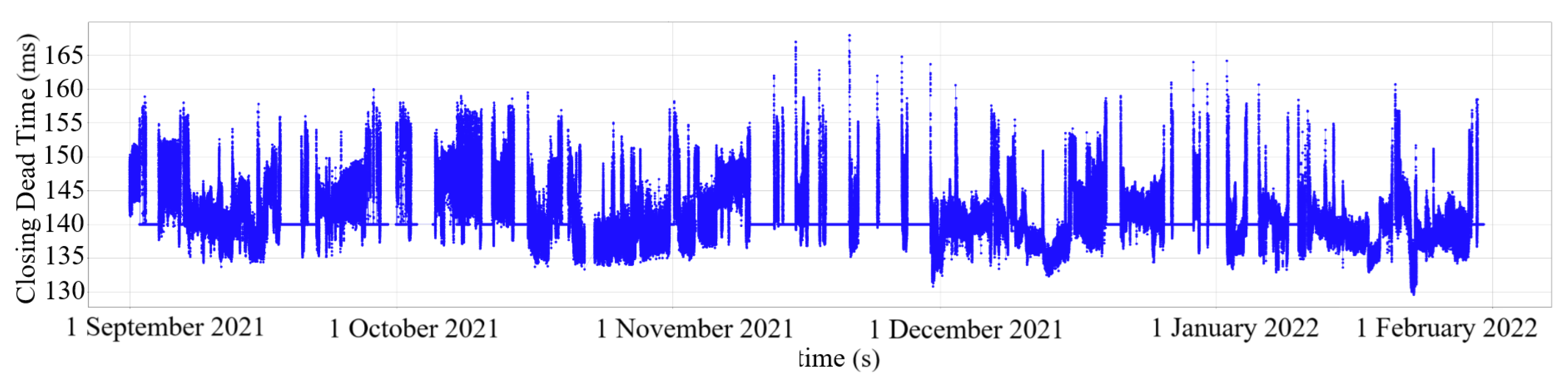
Despite its usefulness, the dataset suffers from several limitations related to temporal resolution, data granularity, and missing key parameters, all of which constrain the depth of analysis and modeling. Specifically, there is one value of the ECDT for each cycle of the engine. Assuming that the rotational speed of the motor is 60 rpm, this corresponds to one ECDT value every second. However, the recording of these values is saved only every 10 s. As a result, most of the ECDT values are not present in the dataset, leading to a significant loss of temporal resolution. Moreover, there are no measurements, such as crank angle or stroke, at the cycle level. Instead, the available data consists of only one ECDT value every 10 cycles. Finally, the average value of ECDT is about 140 ms, which is relatively small compared to the duration of a single cycle, highlighting the fine-scale variability that is not captured by the coarse sampling.

The first step in preparing the data is eliminating outliers. The outliers are a few isolated, extremely high values that are impossible to attain. These outliers were removed by eliminating points with ECDT values higher than a threshold (of 500 ms) and replacing them with an interpolated value. The choice of the threshold was made after visualization of the data and realizing that it was capable of eliminating all the outliers. Figure 5 shows the ECDT for cylinder 1 after removing the outliers.

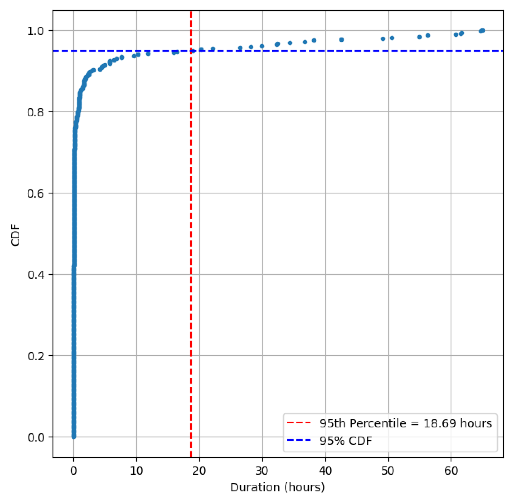
The second step is to identify and select continuous periods of usable data while filtering out intervals with prolonged data absence. Figure 5 shows the presence of some long periods with a constant ECDT equal to 140 ms, indicating the absence of data. To solve this, some periods for study were selected from the 5 months to apply the algorithm. Figure 6 shows the CDF of the duration with the absence of data. Therefore, the top $5\%$ of the periods with the absence of data were eliminated. Then, out of the remaining data periods, the periods longer than 4 days were selected for study and are shown in

Table 3. Periods of study.

Period	Start Time	End Time	Duration
1	2021-09-04 06:10:19	2021-09-17 22:50:04	13 days 16:39:45
2	2021-09-21 22:51:46	2021-09-29 04:14:40	7 days 05:22:54
3	2021-10-05 07:28:14	2021-10-10 12:43:17	5 days 05:15:03
4	2021-10-15 16:33:58	2021-11-09 15:39:13	24 days 23:05:15
5	2021-11-29 21:31:44	2021-12-19 15:44:50	19 days 18:13:06
6	2021-12-21 06:01:05	2021-12-26 03:36:21	4 days 21:35:16
7	2022-01-10 04:45:58	2022-02-01 00:00:00	21 days 19:14:02

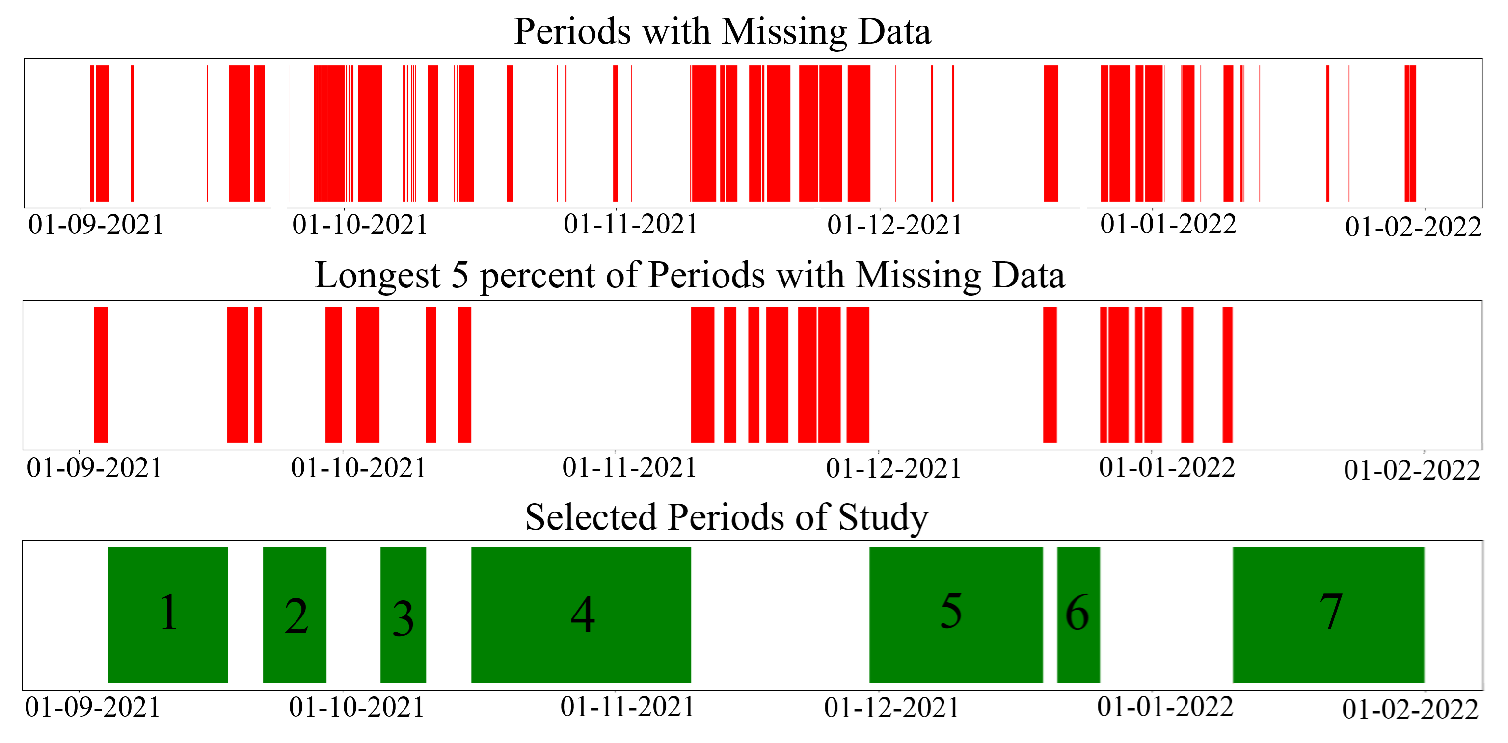
. The format used in the table is for time “YYYY-MM-DD hh:mm:ss” and for duration “DD days hh:mm:ss,” where Y, M, D, h, m, and s represent year, month, day, hour, minute, and second, respectively. Figure 7 shows the periods with missing data and the selected periods for study. Finally, the number of selected periods for study is 7, and it contains 800 K instances for each cylinder with a total duration of 97 days 13:25:21. Overall, the cylinders’ ECDT has a minimum of 122.3 s, a maximum of 191.3 s, an average of 137.65 s, and a standard deviation of 5.09 s.

The aim is to use this data to detect the cylinders with an abnormal ECDT and in which periods. The results from the algorithm are to be compared with abnormalities associated with faults recorded in a technical report shown in Table 2.

7. Results

7.1. Clustering Algorithm

Different clustering algorithms could be adopted in the clustering step of the inner algorithm of CCH-scan. The aim of this section is to analyze the effect of the choice of clustering algorithm and its parameters on the results obtained by CCH-scan. Four clustering algorithms were adopted with different parameters. In each case, the clustering quality Q and the duration of abnormalities D were computed in each scenario as shown in

Table 4. The results of CCH-Scan with different clustering algorithms.

Algorithm (Parameters)	Duration of Abnormality	Clustering Quality
DBSCAN ($\mathcal{N}$ = 2, $ϵ$ = 1.5)	91 days 11:20:00	0.461
DBSCAN ($\mathcal{N}$ = 2, $ϵ$ = 2)	44 days 07:20:00	0.613
DBSCAN ($\mathcal{N}$ = 2, $ϵ$=2.25)	27 days 08:50:00	0.687
DBSCAN ($\mathcal{N}$ = 2, $ϵ$ = 2.5)	13 days 18:00:00	0.76
DBSCAN ($\mathcal{N}$ = 2, $ϵ$ = 3)	1 day 20:10:00	0.892
DBSCAN ($\mathcal{N}$ = 3, $ϵ$ = 1.5)	90 days 19:00:00	0.45
DBSCAN ($\mathcal{N}$ = 3, $ϵ$ = 2)	44 days 07:20:00	0.613
DBSCAN ($\mathcal{N}$ = 3, $ϵ$ = 2.5)	13 days 18:00:00	0.76
Kmeans (K = 2)	92 days 16:30:00	0.485
Kmeans (K = 3)	96 days 01:20:00	0.422
Kmeans (K = 4)	96 days 04:00:00	0.358
Agglomerative ($\mathcal{N}$ = 2)	95 days 04:00:00	0.471
Agglomerative ($\mathcal{N}$ = 3)	97 days 11:40:00	0.412
Agglomerative ($\mathcal{N}$ = 4)	97 days 11:40:00	0.34
Mean Shift (W = 1)	96 days 00:50:00	0.409
Mean Shift (W = 2)	53 days 03:10:00	0.588
Mean Shift (W = 2.25)	32 days 07:50:00	0.667
Mean Shift (W = 2.5)	14 days 16:40:00	0.762
Mean Shift (W = 2.75)	7 days 02:50:00	0.801
Mean Shift (W = 3)	1 day 20:10:00	0.892
Mean Shift (W = 3.25)	0 days 17:00:00	0.901
Mean Shift (W = 3.5)	0 days 00:00:00	-

. The adopted clustering algorithms are DBSCAN, K-means, agglomerative, and mean shift clustering. For the DBSCAN algorithm, two parameters were studied: maximum distance $ϵ$ and minimum number of points $\mathcal{N}$. For K-means, the parameter studied is the number of clusters k. For agglomerative clustering, the studied parameter is the desired number of clusters $\mathcal{N}$. For mean shift clustering, the studied parameter is the bandwidth W. The total number of scenarios is 22.

Looking at the results in Table 4, several observations can be made:

• When K-means was used, the clustering quality decreases with the increase in the number of clusters K.
• When using agglomerative clustering, the clustering quality decreases with the increase in the number of clusters N.
• Better clustering quality can be seen when using DBSCAN and mean shift compared to K-means and agglomerative clustering.
• In DBSCAN, results showed only a slight advantage of using $N=2$ over using $N=3$.
• In DBSCAN, the change in the maximum distance for neighbors $ϵ$ has a great influence on the result. The increase in $ϵ$ increases the quality of clustering and decreases the duration of abnormalities.
• In mean shift clustering, the increase in W increases the quality of clustering and decreases the duration of abnormalities.
• The results of the mean shift algorithm had a slight advantage over DBSCAN.

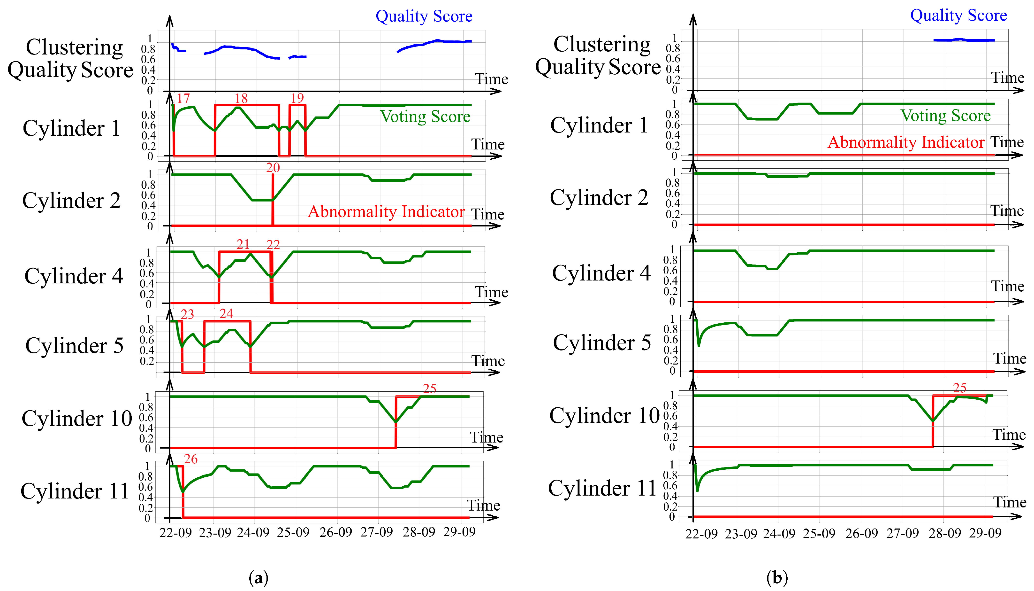
Therefore, in general, changing the parameters of a clustering algorithm could increase the quality of clustering, but the drawback is that this will make the algorithm more selective in detecting abnormalities. As seen in Table 4, the increase in bandwidth in the mean shift algorithm results in limiting the duration of abnormalities. Figure 8 provides insight into the algorithm’s behavior on a period of study, highlighting the voting score and demonstrating the impact of clustering parameter variations on the results. Figure 8a shows the abnormality indicator, quality score, and voting score as a function of time obtained by applying CCH-Scan with mean shift with $W=2.3$ on the period of study 2. As noticed, 10 abnormalities were obtained, having abnormality numbers from 12 to 26. Figure 8b also shows the result of applying CCH-Scan on the second period of study, but this time using the value $W=2.75$ for the mean shift algorithm. In Figure 8b, only one abnormality with the number 25 was obtained. Comparing the results in Figure 8a,b, it is seen that increasing the bandwidth W did not allow the detection of some abnormalities. The abnormalities that were not detected to have lower voting scores and quality scores compared to the abnormality that remained.

There is no perfect choice of the parameters, but certain choices are more reasonable than others. The parameters could be tuned to obtain the most logical outcome. In practice, the choice of the parameters of the algorithms requires experience in the system and statistical analysis, such as knowing how much the estimated duration of abnormalities is. In this study, these statistics are not available.

When looking at the voting score in Figure 8a, it is seen that abnormalities 19, 20, and 22 have a low voting score of around 0.5. This means that the calculations by the inner algorithm did not indicate abnormality for about half of the time. On the other hand, when looking at the voting score for abnormalities 23, 25, and 26, it can be seen that the voting score remained equal to 1 for a period of time. This means that all the calculations by the inner algorithm indicate an abnormality. The information by the algorithm concerning abnormalities 23, 25, and 26 can be trusted more than that concerning abnormalities 19, 20, and 22.

7.2. Discretization Constant

The discretization constant x varies between 0 and 1. It is a threshold that represents the value for which, when the absolute value of the correlation exceeds, the correlation is considered to be sufficient. In this section, the effect of the choice of x on the result of CCH-Scan is discussed. The algorithm was applied with different values of x while using $s=10$ min, $T=24$ h, and mean shift clustering with $W=2.5$.

Table 5. The effect of changing the discretisation constant x.

x	Duration of Abnormality	Clustering Quality
0.4	14 days 21:20:00	0.724
0.5	14 days 16:40:00	0.762
0.6	13 days 10:30:00	0.783
0.7	8 days 08:40:00	0.743
0.8	1 day 22:20:00	0.818

shows the clustering quality and the total duration D of abnormality for different values of the discretization constant x. The results show that as x increases, the clustering quality increases, and the duration of abnormalities decreases. The value $x=0.5$ is the most intuitive choice; however, different values of x could be chosen. Having statistical information concerning the estimated duration of abnormalities, with expertise in the system, allows for a suitable choice of x.

7.3. Changing s and T

The aim is to study how CCH-Scan is affected by the change in the shift s and duration T of the sliding window. The algorithm was applied with different values of s and T while using $x=0.5$ and mean shift clustering with $W=2.5$.

Table 6. Changing of s and T.

T	s	Duration of Abnormality	Clustering Quality
6 h	10 min	8 days 07:00:00	0.771
6 h	30 min	8 days 09:30:00	0.767
6 h	1 h	9 days 03:10:00	0.761
6 h	2 h	10 days 14:10:00	0.756
6 h	4 h	13 days 01:30:00	0.727
12 h	10 min	10 days 21:40:00	0.78
12 h	30 min	11 days 16:50:00	0.776
12 h	1 h	11 days 15:10:00	0.775
12 h	2 h	12 days 04:30:00	0.764
12 h	4 h	12 days 20:30:00	0.745
1 day	10 min	14 days 16:40:00	0.762
1 day	30 min	13 days 21:00:00	0.767
1 day	1 h	13 days 19:20:00	0.762
1 day	2 h	13 days 23:40:00	0.757
1 day	4 h	13 days 09:00:00	0.764
3 days	10 min	28 days 02:20:00	0.735
3 days	30 min	27 days 07:30:00	0.737
3 days	1 h	27 days 03:00:00	0.737
3 days	2 h	27 days 14:00:00	0.735
3 days	4 h	29 days 16:00:00	0.729
3 days	12 h	28 days 00:00:00	0.719

shows the abnormality duration and clustering quality when changing s and T.

The results in Table 6 show that as s gets larger, a slight decrease is observed in the clustering quality and a slight increase in the duration of abnormalities. However, for larger values of T, these variations become insignificant. When s is small enough with respect to T, no more improvement in quality is obtained. Smaller values of s relative to T allow obtaining more results from the inner algorithm, thus yielding more precise results. The increase in T shows a decrease in the quality of abnormalities and an increase in the durations of abnormalities. However, when the duration of T is small enough, these changes become insignificant.

7.4. Analysis of Abnormalities

CCH-Scan was applied with $s=10\min$ and $T=1\mathrm{day}$ while using $x=0.5$ and mean shift clustering with $W=2.3$. The number of abnormalities obtained is 79. An abnormality ${\mathcal{F}}_w$ is characterized by its duration $e_w-s_w$, the degree of abnormality ${\mathcal{A}}_w$, the quality score of abnormality ${\mathcal{S}}_w$, and the voting score of abnormality ${\mathcal{V}}_w$. Based on these characteristics, abnormalities could be queried or filtered, and several statistics could be computed. For example, abnormalities with very short durations may be removed from the analysis.

Table 7. Statistics related to the characteristics of abnormalities.

Parameter	${\mathit{e}}_{\mathit{w}}-{\mathit{s}}_{\mathit{w}}$	${\mathcal{S}}_{\mathit{w}}$	${\mathcal{V}}_{\mathit{w}}$	${\mathcal{A}}_{\mathit{w}}$
average	16.36h	0.66	0.679	0.548
std	12.9h	0.095	0.118	0.241
minimum	0h	0.386	0.5	0.05
Q1	3.5h	0.61	0.59	0.321
Median	15.5h	0.665	0.667	0.573
Q3	23.83h	0.727	0.779	0.754
maximum	47.33h	0.869	0.917	0.888

shows some statistics related to the obtained abnormalities.

These statistics can serve as a reference to help characterize and compare a specific abnormality to the general characteristics of the obtained abnormalities. For example, the average duration $e_w-s_w$ for an abnormality is 16.36 h, with an average degree of abnormality ${\mathcal{A}}_w$ equal to 0.548.

To obtain the most abnormal signals, it is possible to focus on the degree of abnormality ${\mathcal{A}}_w$. For example,

Table 8. Abnormalities: top 10 percent degree of abnormality.

w	${\mathit{s}}_{\mathit{w}}$	${\mathit{e}}_{\mathit{w}}$	${\mathcal{Z}}_{\mathit{w}}$	${\mathcal{S}}_{\mathit{w}}$	${\mathcal{V}}_{\mathit{w}}$	${\mathcal{A}}_{\mathit{w}}$
3	2021-09-17 19:50:19	2021-09-17 22:40:19	1	0.665	0.844	0.888
8	2021-09-17 19:50:19	2021-09-17 22:40:19	2	0.665	0.844	0.888
11	2021-09-17 19:50:19	2021-09-17 22:40:19	4	0.665	0.844	0.888
57	2021-12-18 15:11:44	2021-12-19 15:41:44	1	0.744	0.838	0.875
58	2021-12-18 15:11:44	2021-12-19 15:41:44	2	0.744	0.838	0.875
59	2021-12-18 15:11:44	2021-12-19 15:41:44	5	0.744	0.838	0.875

shows the abnormalities with the top 10 percent degree of abnormality ${\mathcal{A}}_w$. Looking at this table, it can be seen that the top 3 abnormalities ($w=3$, 8, and 11) happened at the same time on 2021-09-17 between 19:50:19 and 22:40:19.

Sometimes, the algorithm detects abnormalities but with low confidence in the results. For example,

Table 9. Abnormalities with the least 10 voting score and quality score.

w	${\mathit{s}}_{\mathit{w}}$	${\mathit{e}}_{\mathit{w}}$	${\mathcal{Z}}_{\mathit{w}}$	${\mathcal{S}}_{\mathit{w}}$	${\mathcal{V}}_{\mathit{w}}$	${\mathcal{A}}_{\mathit{w}}$
20	2021-09-24 09:21:46	2021-09-24 09:21:46	2	0.552	0.5	0.3
22	2021-09-24 09:21:46	2021-09-24 09:21:46	4	0.552	0.5	0.3
37	2021-11-02 10:03:58	2021-11-02 18:03:58	4	0.532	0.507	0.463
46	2021-11-09 15:13:58	2021-11-09 15:13:58	7	0.386	0.5	0.442
54	2021-11-09 15:13:58	2021-11-09 15:13:58	11	0.386	0.5	0.442
60	2021-12-16 00:41:44	2021-12-16 13:31:44	6	0.541	0.543	0.256

shows the abnormalities with the minimum 10 percent quality score ${\mathcal{S}}_w$ and voting scores ${\mathcal{V}}_w$. These abnormalities could be neglected when analyzing the results.

Statistics can also be performed at the cylinder level. This helps in indicating where necessary maintenance action should be prioritized.

Table 10. Statistics about cylinders.

Cylinder	Number of Abnormalities	Abnormalities Duration	Abnormality
1	14	9 days 14:20:00	0.759
2	13	9 days 13:50:00	0.562
4	15	9 days 03:40:00	0.559
5	12	9 days 05:20:00	0.438
6	1	0 days 12:50:00	0.256
7	6	2 days 05:00:00	0.332
8	4	4 days 14:00:00	0.292
10	3	3 days 11:10:00	0.077
11	7	2 days 21:00:00	0.453
12	4	2 days 15:30:00	0.366

shows the number of abnormalities, total abnormality duration, and degree of abnormality corresponding to each cylinder. Looking at the results, it can be seen that cylinders 3 and 9 did not have any abnormalities during the period of study. Cylinders 6, 7, 8, 10, and 12 showed a low level of abnormality. However, cylinders 1, 2, 4, 5, and 11 exhibited a serious degree of abnormality, indicating that necessary actions need to be taken. These results show high consistency with the reported findings in Table 2.

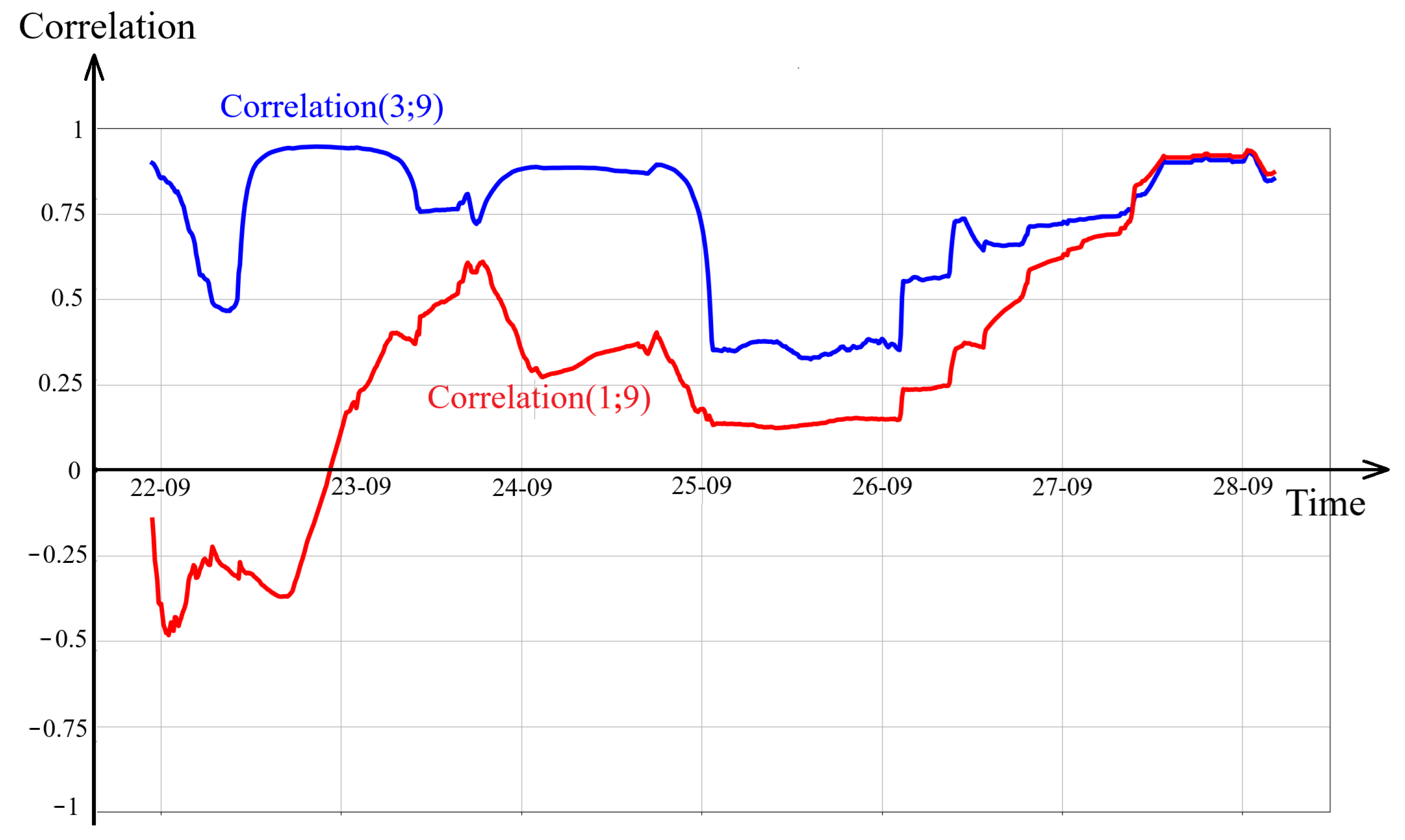
Figure 9 shows the correlation as a function of time for the second study period between the ECDT of cylinders 3 and 9 (in blue) and between cylinders 1 and 9 (in red). It is seen that the correlation between the ECDT of cylinders 3 and 9 is high during the second period of the study, as defined in Table 3. This is consistent with the fact that these two cylinders did not show any abnormalities. The correlation between cylinder 1, which showed a high degree of abnormality, and cylinder 9, which did not show any abnormality, is low for the majority of period 2.

As mentioned before, a fault is a defect or malfunction within a system component that causes improper operation or failure to meet performance standards, often linked to specific components or subsystems. The technical report documented 4 faults, as shown in Table 2. Each of these faults was linked to abnormalities in the ECDT of some cylinders. However, abnormalities represent deviations from normal behavior but do not always indicate faults. Observing a pattern of abnormalities may indicate the presence of underlying faults.

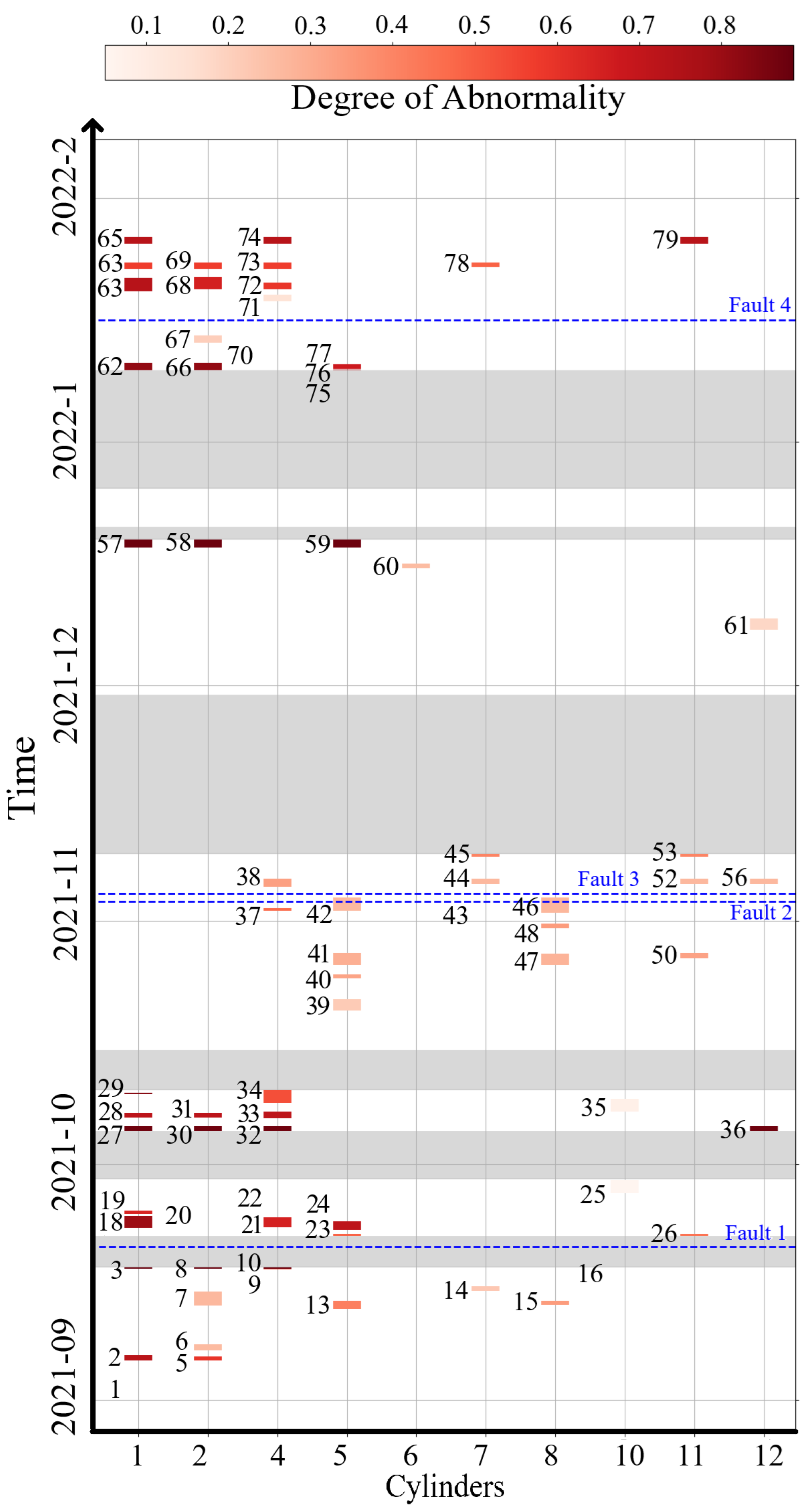
The obtained abnormalities could be plotted as a function of time to observe which groups of abnormalities occurred around the same period and compare the results to the reports. Figure 10 shows a timeline of the abnormalities obtained by CCH-Scan and the corresponding degree of abnormality.

Looking at the results, it can be seen that the abnormalities obtained by CCH-Scan are grouped into three main clusters based on the time of occurrence. These groups can be mapped to the four faults reported in Table 2. For example, the obtained abnormalities with $1\le w\le 36$ can be related to “Fault 1”, abnormalities with $37\le w\le 56$ can be associated with “Fault 2” and “Fault 3”, and abnormalities with $57\le w\le 79$ (except for abnormalities 60 and 61) can be linked to “Fault 4”.

It is also noticeable that during the first 18-day period, no significant abnormalities were detected, which aligns with the reports on faults.

“Fault 1” in the report indicates faults in cylinders 1, 2, 5, and 11, and this is consistent with the plot. However, the plot also shows several other serious abnormalities that were not reported, such as in cylinder 4. “Fault 2” and “Fault 3” from the report indicate faults in cylinders 4 and 8, which were detected by the algorithm, but the algorithm also identified issues in other cylinders that were not reported.

Although the ground truth from the technical reports is not complete and fully reliable, there is a high degree of alignment with the results obtained by the algorithm.

8. Conclusions

This paper introduces CCH-Scan, a novel anomaly detection algorithm designed to analyze correlated signals in normal operating conditions. The algorithm applies a clustering technique to correlation matrices derived from signal sets within specific short time intervals, repeating this process over the study period. The methodology and algorithm details are thoroughly explained.

CCH-Scan was applied to exhaust valve closing dead time (ECDT) signals to detect abnormalities in a 12-cylinder marine dual-fuel engine. The significance of this critical signal in the exhaust system of a marine dual-fuel engine is highlighted. The algorithm includes several parameters—such as the clustering algorithm, discretization constant, shift (s), and duration (T)—which influence the results, particularly the duration and quality of detected abnormalities. The effect of varying these parameters was explored within the case study.

While there is no one-size-fits-all set of parameters, the optimal choice depends on the specific application and expert knowledge of the system. Abnormalities were identified, analyzed, and plotted over time, revealing the time of occurrence and degree of abnormality. These results were compared with a technical maintenance report, showing a high degree of consistency. The detected abnormalities were grouped into three categories, each corresponding to a distinct fault.

Despite the modest reliability of ground truth data typical in industrial projects, CCH-Scan demonstrated promising potential for diverse applications. While the algorithm showed strong performance, its numerous parameters may present challenges in tuning. Future work will focus on comparing CCH-Scan with other methods in varied environments to enhance its understanding and broaden its applicability.

Future research will address several open challenges and opportunities for advancing CCH-Scan. Key directions include improving parameter sensitivity analysis and developing parameter tuning strategies. Further validation across different types of machinery and operational contexts is important. Additionally, efforts will be made to evaluate the algorithm’s performance under noisy conditions and with missing or incomplete data. Quantitative benchmarking of CCH-Scan against established anomaly detection techniques will be pursued once more accurate ground truth data becomes available. Finally, investigations into real-time applicability will be crucial to extending the algorithm’s utility in industrial environments.