Performance Prediction of the Gearbox Elastic Support Structure Based on Multi-Task Learning

Abstract

The gearbox, as an important transmission component in wind turbines, connects the blades to the generator and is responsible for converting wind energy into mechanical energy and transmitting it to the generator. Its ability to reduce vibrations directly affects the operational lifespan of the wind turbine. When designing the gearbox’s elastic support structure, it is essential to evaluate how the design parameters influence various performance metrics. Neural networks offer a powerful means of capturing and interpreting the intricate associations linking structural parameters with performance metrics. However, conventional neural networks are usually optimized for a single task, failing to fully account for task differences and shared information. This can lead to task conflicts or insufficient feature modeling, which in turn affects the learning efficiency of inter-task correlations. Furthermore, physical experiments are costly and provide limited training, making it difficult to meet the large-scale dataset requirements for neural network training. To address the high cost and limited scalability of traditional physical testing for gearbox rubber damping structures, in this study, we propose a low-cost performance prediction method that replaces expensive experiments with simulation-driven dataset generation. An optimal Latin hypercube sampling technique is employed to generate high-quality data at minimal cost. On this basis, a multi-task prediction model called multi-gate mixture-of-experts with LSTM (PLE-LSTM) is constructed. The adaptive gating mechanism, hierarchical nonlinear transformation, and effective capture of temporal dynamics in the LSTM significantly enhance the model’s ability to model complex nonlinear patterns. During training, a dynamic weighting strategy named GradNorm is utilized to counteract issues like the early stabilization in multi-task loss convergence and the uneven minimization of loss values. Finally, ablation experiments conducted on different datasets validate the effectiveness of this approach, with experimental results demonstrating its success.

1. Introduction

The tower height and rotor diameter of high-power wind turbines are often tens or even hundreds of meters. To ensure good mechanical performance and vibration reduction effects, vibration-damping components need to be installed in key parts of the wind turbine [1]. The elastic support of the gearbox is a crucial component of the wind turbine’s elastic support system, and its structural–mechanical properties directly affect the vibration reduction performance and service life of the wind turbine’s damping system. Therefore, structural–mechanical performance metrics have always been a key focus during the design of the gearbox’s elastic support in wind turbines.

With the development of computer science and the improvement of hardware capabilities, simulation experiments have become a widely recognized method for replacing physical experiments and acquiring real-world data [2]. Many researchers have used simulation experiments to study the relationship between design parameters and performance metrics. For instance, Kai Yang et al. conducted finite element analysis of the bone grinding process with SolidWorks 2018 and Abaqus 2023 to investigate the effects of various parameters on grinding forces, and they validated their findings through physical experiments [3]. Chao Zheng et al. conducted a three-dimensional multi-body contact nonlinear finite element analysis based on the Mooney–Rivlin constitutive model. They systematically investigated the effects of key parameters, including thickness, height, and rubber hardness, on the sealing performance of hydrogenated nitrile rubber, providing valuable insights for the design of future sealing components [4]. Analytical frameworks derived from simulation experiments are capable of accurately capturing the correlation among design variables and performance metrics. However, traditional models often have limitations when dealing with complex data and revealing underlying nonlinear relationships. Therefore, there is an urgent need to explore more advanced modeling approaches.

Recently, the application of machine learning techniques in engineering has gradually increased, and neural networks have been widely applied in engineering design. Compared to traditional modeling methods, neural networks demonstrate more significant advantages in handling complex data and uncovering nonlinear relationships [5]. Xiaoyu Huang et al. used an improved sparrow algorithm to optimize machine learning models for predicting the relative dynamic elastic modulus of rubber concrete in order to investigate its durability. They also verified the rationality of the developed model through a sensitivity analysis using CAM [6]. D. Pan et al. proposed a modeling method that trains neural networks with experimental data. The characteristic parameters of dampers were used as the input to the neural network model, with the damping force as the output. Numerical simulation examples were provided, demonstrating that the method can effectively predict damper performance [7]. Liangcheng Dai et al. combined physical parameter models with neural network models and proposed an accurate hybrid neural network model for hydraulic dampers to simulate their dynamic performance under various working conditions. The model’s accuracy was verified by comparing its results with experimental results [8]. These research findings indicate that machine learning has broad potential for improving the accuracy of engineering design and performance prediction.

However, engineering design often involves numerous design parameters and performance metrics. In these scenarios, employing conventional neural network frameworks—Such asBP [9], RBF [10], and GRNN [11]—to study the link between design variables and performance measures frequently results in unsatisfactory outcomes. The unsuitability of traditional neural networks for multi-task scenarios primarily stems from their lack of effective inter-task sharing mechanisms and discrimination capabilities. These networks are typically optimized for a single task, failing to fully account for task differences and shared information, which leads to task conflicts or insufficient feature modeling [12]. While methods such as model fusion and ensemble learning can handle multiple tasks, these approaches mainly combine the results of independent tasks and fail to effectively consider the interactions between tasks [13]. Moreover, neural network training depends heavily on datasets, but most data on rubber vibration-damping components currently come from experiments, which are costly and result in a limited sample size. Research on the relationship between design parameters and performance metrics for rubber vibration-damping components based on a multi-task learning framework is still relatively scarce.

In order to mitigate the challenges stemming from restricted datasets, Yuexing Han et al. proposed an improved HP-VAE-GAN method for generating material images to achieve data augmentation, and they validated the method’s effectiveness through texture experiments on similar material images [14]. Christopher Bowles et al. utilized generative adversarial networks (GANs) to generate synthetic samples with a realistic appearance in order to enhance training data, demonstrating the feasibility of introducing GAN-generated synthetic data into training datasets for two brain segmentation tasks [15]. However, GANs and VAEs are currently primarily used for image generation and prediction, with their application in other types of tasks still limited. To reduce experimental costs, many researchers have generated datasets based on simulation experiments. Mahziyar Darvishi et al. conducted a finite element analysis (FEA) to study materials with different honeycomb structures and used corresponding analytical equations to validate the results, thus creating the datasets needed for machine learning algorithms to select the optimal honeycomb structure [16]. Defu Zhu et al. established sandstone sample data based on a finite element analysis and used a machine learning model optimized via particle swarm optimization to predict the shear strength parameters of sandstone [17]. Datasets generated from simulation experiments can significantly reduce costs and experimental time; however, issues such as the error between simulation experiments and real experiments, as well as the choice of sampling method for the dataset, still impact their quality. These issues need to be further addressed.

Compared to traditional neural networks, multi-task learning (MTL) networks enhance model performance by sharing learning structures across multiple related tasks [18], as demonstrated in models such as MMOE [19], PLE [20], and CSN [21]. In practical applications, Fei Luo et al. improved the accuracy and robustness of cross-regional wind energy and fossil fuel power generation forecasts based on an enhanced MMOE model, and they validated the model’s advantages through benchmark experiments [22]. Jiaobo Zhang et al. designed a cross-stitch attention network (CACSNet) based on shared attention mechanisms, demonstrating excellent performance in gas porosity prediction. Additionally, detailed ablation experiments and parameter analysis further validated the effectiveness of the structure [23]. As separate models do not need to be built or optimized for each task, MTL models require fewer parameters. More importantly, when a single model is trained to perform multiple tasks simultaneously, it should be able to work synergistically, thereby revealing common latent structures. This allows the model to achieve better single-task performance, even when the dataset for each task is limited [24]. Although MTL has achieved impressive results regarding its generalization to multiple tasks, existing MTL research still primarily relies on manually designed features or parameter sharing at the problem level [25]. To avoid gradient conflicts between tasks, which is a common issue in MTL, researchers have increasingly recognized the importance of finding appropriate weighting strategies for MTL. This ensures that the overall experience loss is minimized without sacrificing the learning performance of individual tasks [26]. Therefore, optimizing the loss function in multi-task learning is crucial.

To address the issues in datasets and multi-task learning neural networks, in this study, we propose an optimized Latin hypercube sampling method based on a digital twin model of a gearbox elastic support combined with simulation experiments to generate the dataset required for the neural network. This approach balances the relationship between experimental cost and dataset quality. The effectiveness of the simulation experiment is validated through physical experiments. Given the complexity and nonlinear characteristics of structured data for gearbox elastic support, we introduce an improved PLE-LSTM neural network. Based on the PLE model framework and leveraging the nonlinear modeling capabilities of the LSTM module, the prediction accuracy of the entire neural network is enhanced. To resolve issues such as gradient conflicts and imbalance between tasks in multi-task learning, the GradNorm optimization algorithm is incorporated to dynamically weight the loss functions of each task, thereby coordinating the learning process between tasks and improving the overall performance of the model. The main contributions of this study are as follows:

Based on a digital twin model of gearbox elastic support, an optimized Latin hypercube sampling method is proposed, combined with simulation experiments to generate the dataset required for the neural network, significantly saving experimental costs and time.

An improved PLE-LSTM neural network based on the PLE model framework is proposed, effectively capturing and extracting the complexity and nonlinear characteristics of the structured data of the gearbox elastic support.

The GradNorm optimization algorithm is incorporated to dynamically weight the loss functions of each task, optimizing the learning process between tasks and thereby improving the model’s overall effectiveness.

The effectiveness of the proposed method is validated through ablation experiments on different datasets. The experimental results show that, with the same sample size, the proposed method outperforms traditional methods, achieving better results.

2. Method

In this section, we first introduce the data generation method based on optimal Latin hypercube sampling combined with finite element simulation experiments. Then, we introduce the refined PLE-LSTM network design derived from the PLE multi-task framework. Lastly, we detail the strategy for enhancing loss functions for multiple tasks through GradNorm. The overall framework is shown in Figure 1.

2.1. Dataset Generation

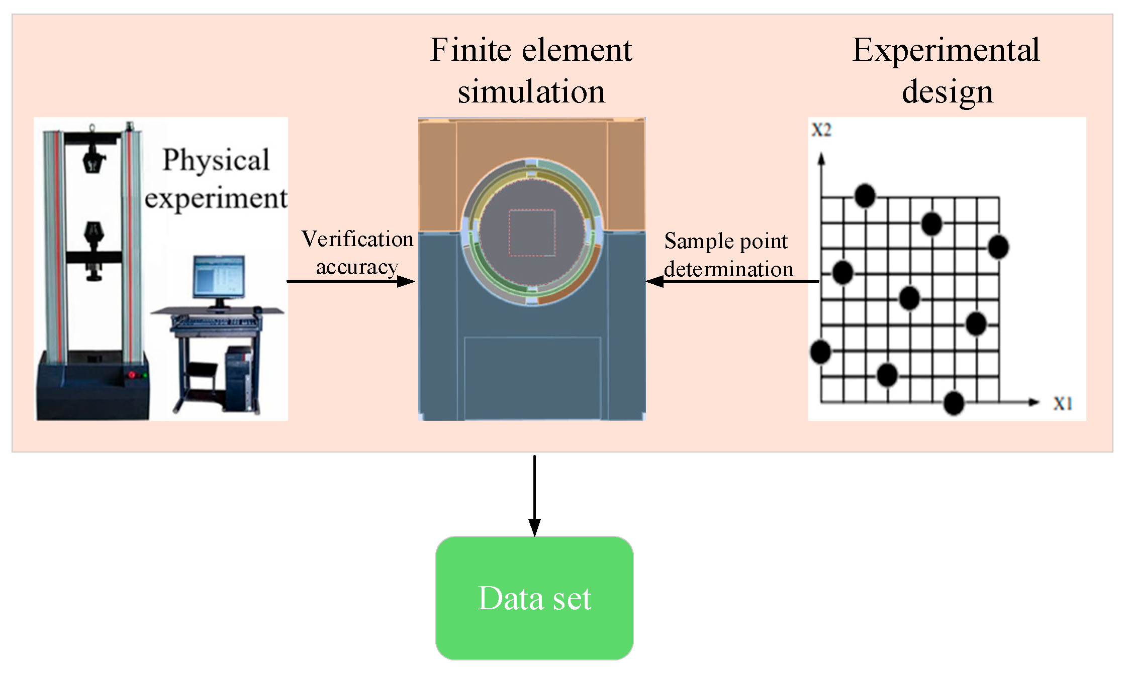
In the industrial field, dataset generation through physical experiments is often costly, time-consuming, and difficult to scale or repeat, with outcomes heavily dependent on specific conditions and equipment. These limitations hinder the exploration of extreme scenarios and reduce the generalizability of the data. Although simulation experiments offer a more cost-effective and flexible alternative, inherent discrepancies between real-world results can compromise dataset integrity and affect the training efficiency of network models. To address these challenges, in this study, we propose a cost-efficient dataset generation method that integrates simulation experiments with optimal Latin hypercube sampling, effectively balancing performance, generalizability, and reliability. The overall process of this method is illustrated in Figure 2.

2.2. Optimal Latin Hypercube Sampling

Latin hypercube sampling (LHS) is a widely used statistical method in numerical simulation and experimental design, with the aim of achieving efficient sampling in high-dimensional parameter spaces. This method was first introduced by M.D. McKay, R.J. Beckman, and W.J. Conover. The basic idea is that it assumes a known functional relationship between input variables $x_1,\dots ,x_s$ and the output response:

$$Y=f\left(x_1{\dots x}_s\right),x=\left(x_1{\dots x}_s\right)\in C^s$$

(1)

Assuming that the experimental region is a unit cube $C^s={\left[\mathrm{0,1}\right]}^s$, the total mean of variable $y$ over $C^s$ is:

$$E\left(y\right)={\int }_{c^s}f\left(x_1{\dots x}_s\right){dx}_1\dots {dx}_2$$

(2)

If $n$ experimental points $z_1,\dots ,z_n$, are selected in $C^s$, the mean of $y$ at these $n$ experimental points is given by:

$$\overline{y}\left(D_n\right)={\displaystyle \frac{1}{n}}\sum _{i=1}^{n}f\left(z_i\right)$$

(3)

Here, $D_n$ = {$z_1,\dots ,z_n$} represents a design consisting of $n$ points. The Latin hypercube design selects $D_n$ using a sampling method such that the corresponding estimate $\overline{y}\left(D_n\right)$ is unbiased, i.e.,

$$E\left(\overline{y}\left(D_n\right)\right)=E\left(y\right)$$

(4)

From the above inference, it can be concluded that the Latin hypercube design uses an equal-probability stratified sampling method, which has excellent spatial filling capabilities within the entire range of input parameter distributions and their domains. The parameter samples generated by this method are highly representative. Compared to other design methods, the Latin hypercube design can achieve the desired research objectives with fewer samples.

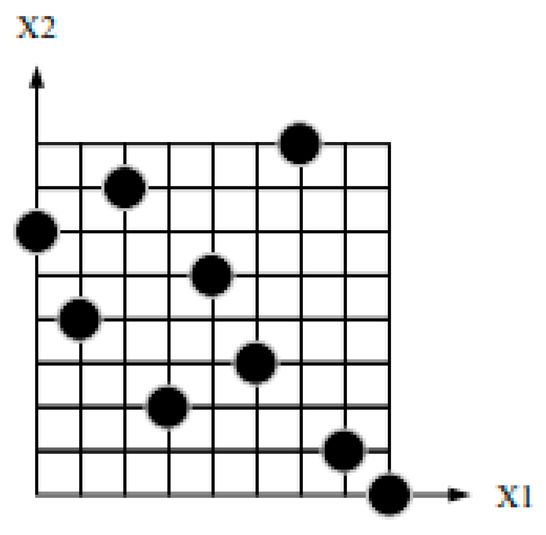
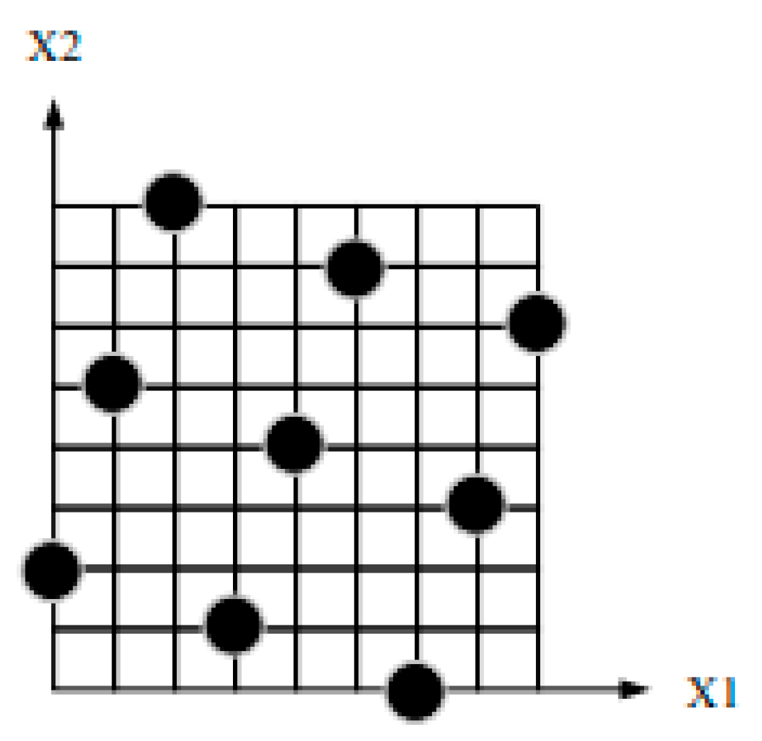
Optimal Latin hypercube design is an improvement of the Latin hypercube design, further enhancing the uniformity of sampling and improving the data fitting accuracy. It demonstrates better spatial filling capabilities and balance. For example, in the case of a two-factor, nine-level analysis sample, the two methods differ in the number of sample points collected and their distribution, as shown in Figure 3 and Figure 4.

As shown in the comparison chart, Latin hypercube sampling (LHS) ensures uniform sampling across individual dimensions but relies on basic stratified sampling, which may lead to sample clustering or gaps in high-dimensional spaces. In contrast, optimal Latin hypercube sampling (OLHS) mitigates these issues by providing a more uniformly distributed sample set. With its optimized coverage, OLHS better spans the parameter space and reduces redundancy. As a result, for the same sample size, OLHS offers improved spatial coverage and representativeness, enhancing dataset quality and boosting model training efficiency and prediction accuracy.

2.3. Multi-Task Learning Network Framework

Multi-task learning (MTL) network models are a type of machine learning framework designed to enhance the model’s generalization ability and performance by simultaneously learning multiple related tasks. The core idea is to leverage the relationships between different tasks, promoting the joint learning of features through shared representations, thereby improving the predictive ability of each individual task.

Traditional multi-task learning faces two main issues: one is the “balancing” problem (also known as the “teeter-totter” problem), and the other is negative transfer.

(1)

The “teeter-totter” problem: In multi-task learning, when the correlation between tasks is complex, improving the performance of one task may be accompanied by a decline in the performance of others. In other words, multiple tasks cannot be improved simultaneously, and the performance may be worse than when modeled separately.

(2)

Negative transfer: The performance of multi-task learning is worse than training each task separately, as joint training leads to a decline in task performance. This phenomenon is more pronounced when the tasks have weak or even conflicting correlations.

To address the issue of negative transfer, the cross-stitch network learns static linear combinations to fuse task representations but fails to capture sample-dependent dynamic changes. The MMoE model combines gating and expert networks to handle task correlations but overlooks the differences and interaction information among experts. In contrast, the PLE model reduces harmful parameter interference by sharing experts and task-specific experts, and it uses multi-layer experts and gating networks to extract deep features in the lower layers while separating task-specific parameters in the higher layers. This effectively captures complex task correlations and improves model performance.

In the PLE framework, the CGC module serves as the core, incorporating specialized expert modules in the lower layers and task-specific tower networks in the upper layers. Each expert module consists of multiple sub-networks—referred to as experts—whose number is controlled by a hyperparameter. The tower networks are also multi-layered, with their depth and width being configurable. Shared experts are responsible for learning common patterns across tasks, while task-specific experts focus on features unique to each task. Each tower integrates knowledge from both the shared and task-specific experts. Consequently, the shared experts are trained using data from all tasks, whereas the task-specific experts are updated exclusively with data from their respective tasks. The structure of the CGC network is illustrated in Figure 5.

As illustrated above, within the CGC framework, common experts and task-oriented specialists are selectively integrated using a gating mechanism. The structure of the gating network is based on a single-layer feedforward network with SoftMax as the activation function. The input to the gating network is the selector, which computes the weighted sum of the selected vectors, i.e., the output of the experts. More precisely, the output of the gating network for task k is represented as:

$$g^k\left(x\right)=w^k\left(x\right)S^k\left(x\right)$$

(5)

Here, $x$ is the input representation, and $w^k\left(x\right)$ is the weighting function, which calculates the weight vector for the task through a linear transformation followed by a SoftMax layer.

$$w^k\left(x\right)=Softmax\left(W_g^{k}x\right)$$

(6)

In this equation, $w^k\left(x\right)\in R^{\left(m_{k+}{m}_s\right)\times d}$, $m_k\mathrm{a}\mathrm{n}\mathrm{d}{m}_s$ are the numbers of shared experts and task-specific experts for task k, respectively, and d is the dimensionality of the input representation $S^k\left(x\right)$, which is the selected matrix composed of all selected vectors, including both the shared experts and task-specific experts for task k:

$$S^k\left(x\right)={\left[{E^T}_{\left(k,1\right)},{E^T}_{\left(k,1\right)},\dots ,{E^T}_{(k,m_{k)}},{E^T}_{\left(s,1\right)}{E^T}_{\left(s,2\right)},\dots ,{E^T}_{(s,m_{s)}}\right]}^T$$

(7)

Finally, the prediction for task k is given by:

$$y^k\left(x\right)=t^k\left(g^k\left(x\right)\right)$$

(8)

Here, $t^k$ represents the tower network for task k.

CGC removes the connections between task-specific towers and experts with other tasks, reducing interference. At the same time, by combining the advantages of the dynamic fusion of input representations through the gating network, CGC better handles the balance between tasks and sample dependencies.

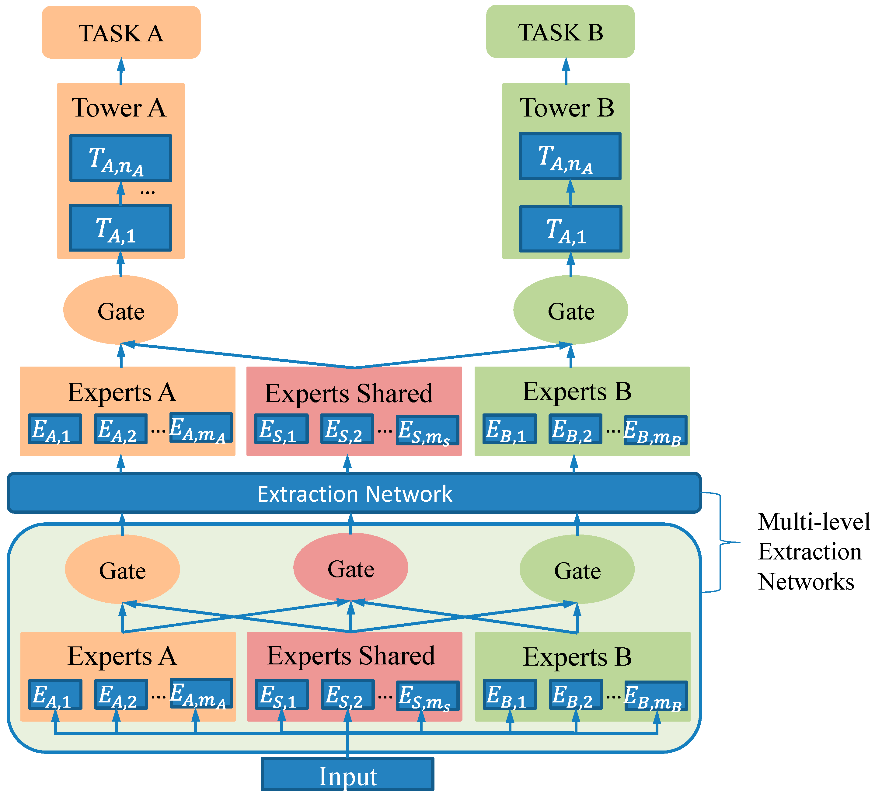
PLE (progressive layered extraction) constructs a feature extraction network through multiple layers of CGC (completely shared gate-controlled) connections to progressively extract higher-order shared information. This network not only designs gating networks for task-specific experts but also introduces gating networks for shared experts to integrate the knowledge of all experts in each layer. In this configuration, the task parameters in PLE are not completely isolated in the initial stages as they are in CGC; instead, they become progressively differentiated through deeper network layers. Moreover, the gating mechanisms in the upper feature extraction layers depend on the integrated outputs from lower-layer gating systems rather than on the direct processing of the raw input, thereby offering more targeted guidance for the abstract representations generated by the higher-level experts. The structure of the PLE network is illustrated in Figure 6.

In PLE, the weight function, selection matrix, and gating network calculations are the same as in CGC. Specifically, in the j-th extraction network of PLE, the gating network for task k is represented as:

$$g^{k,j}\left(x\right)=w^{k,j}{(g}^{k,j-1}\left(x\right)\left)S^{k,j}\right(x)$$

(9)

In the equation, $w^{k,j}$ is the weighting function for the task, and ${g^{k,j-1}S}^k$ serve as the outputs. j represents the matrix selected by task $k$ in the j-th extraction network.

After computing all the gating networks and experts, the final prediction for task k in PLE is given by:

$$y^k\left(x\right)=t^k\left(g^{k,N}\left(x\right)\right)$$

(10)

PLE (progressive layered extraction) adopts a progressive separation routing mechanism, which comprehensively absorbs information from lower-level experts, gradually extracts higher-level shared knowledge, and progressively separates task-specific parameters. During the process of knowledge extraction and transformation, PLE uses higher-level shared experts to jointly extract, aggregate, and route lower-level representations. This not only captures shared knowledge but also progressively allocates it to the tower layers of specific tasks. This mechanism enables more efficient and flexible joint representation learning and knowledge sharing, significantly enhancing the adaptability and performance of multi-task learning.

2.4. LSTM Neural Network

Long short-term memory (LSTM) is a special type of recurrent neural network (RNN) designed to address the vanishing gradient problem faced by traditional RNNs when processing long sequences. It effectively retains and processes long-term dependencies through a unique gating mechanism. The core of LSTM consists of a unit that includes a forget gate, an input gate, and an output gate. Each gate is a special structure that controls the flow of information. Its internal structure is shown below Figure 7.

The computational formula of the LSTM neural network model is as follows:

$$\left\{\begin{array}{c}{i}_t=\sigma (W_x{x}_i+W_{hi}{h}_{i-1}+W_{ci}{c}_{i-1}+b_i)\\ f_t=\sigma (W_{xf}{x}_t+W_{hf}{h}_{i-1}+W_{fi}{c}_{t-1}+b_f)\\ c_t=f_t{h}_{t-1}+i_t\times tanh\left(W_{xc}x+W_{hc}{h}_{i-1}+b_c\right)\\ o_t=\sigma (W_{xo}{x}_t+W_{ho}{h}_{t-1}+W_{co}{c}_i+b_o)\\ h_t=o_{t}tanh\left(c_t\right)\end{array}\right.$$

(11)

Here, $\sigma$ denotes the nonlinear Sigmoid function; $i_t$ represents the input gate; $f_t$ represents the forget gate; $c_t$ is the updated cell state; $o_t$ is the output gate; $x_t$ is the input information; $h_t$ is the output information obtained; $W$ represents the respective weights; and $b$ represents the corresponding bias terms.

LSTM, with its flexible gating mechanism, multi-level nonlinear feature transformations, and efficient capture of temporal dynamic patterns, is able to precisely model complex nonlinear dependencies in long sequences while adapting to the diversity and complexity of the data. Due to these advantages, LSTM excels in many nonlinear data modeling tasks.

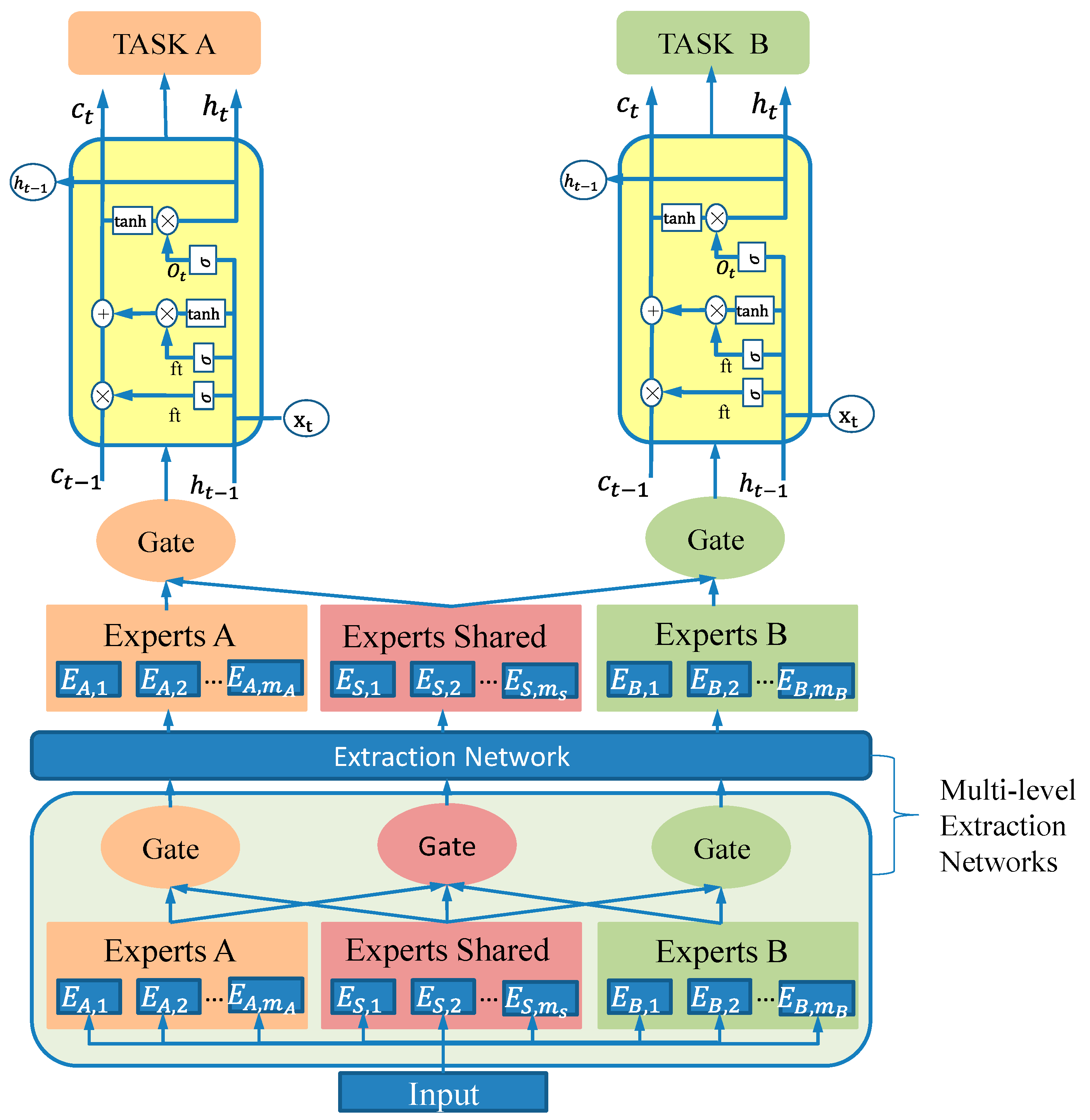
2.5. PLE-LSTM Neural Network

In contrast to the PLE network model framework, PLE-LSTM substitutes the tower layer, which is responsible for fitting the output of each task, with an LSTM neural network. The framework of the PLE-LSTM model is illustrated in Figure 8.

Given that the hyperelastic rubber materials used in gearbox elastic supports exhibit strong nonlinearity and large deformations, replacing the PLE model’s tower layer with an LSTM network can greatly enhance its ability to model such behavior. LSTM’s gating mechanism and nonlinear activation functions allow it to capture complex task-specific nonlinear dependencies. Additionally, its dynamic weighting of short- and long-term information improves robustness to noise and data variability. By leveraging LSTM’s state accumulation, the tower layer can better extract and integrate features from shared and task-specific experts, leading to more representative high-level features and improved multi-task prediction performance.

2.6. Multi-Task Loss Function Based on GradNorm

In multi-task learning, due to significant differences in importance, scale, and other factors between tasks, directly combining losses by linearly weighting the loss functions may cause the loss of certain tasks to dominate, thereby suppressing the learning of other tasks and negatively impacting the overall model performance.

GradNorm is a method that calculates task sample weights based on gradient loss, decreasing the sample weight of tasks with a fast learning speed and increasing the sample weight of tasks with a slow learning speed. This helps to balance the learning speeds of different tasks, thereby improving the sufficiency of task learning. GradNorm dynamically adjusts sample weights based on the learning speed of each task, thus introducing a temporal dimension to the sample weights. The faster the loss decreases, the faster the task converges during the learning process. The basic principle of GradNorm is as follows.

First, the variables $G_W^{\left(i\right)}\left(t\right),\overline{G_W}\left(t\right)$ are introduced, and the gradient of the loss is measured:

$$G_W^{\left(i\right)}\left(t\right)={\left|\left|{\nabla }_{w{W}_i}\left(t\right)L_i\left(t\right)\right|\right|}_2$$

(12)

$$\overline{G_W}\left(t\right)=E_{task}\left[G_W^{\left(i\right)}\left(t\right)\right]$$

(13)

Here: $G_W^{\left(i\right)}\left(t\right)$ is the gradient normalization value of task i, and it is the product of the weight $w_i\left(t\right)$ of task i and loss $L_i\left(t\right)$ of task i, with respect to the L2 norm of parameter W. The larger the value of $G_W^{\left(i\right)}\left(t\right)$, the larger the loss magnitude of that task.

$\overline{G_W}\left(t\right)$ is the global gradient normalization value (i.e., the expected value of the gradient normalization values of all tasks).

Next, variable $r_i\left(t\right)$ is defined to measure the learning speed of task i,

$$\widetilde{L_i}\left(t\right)={\displaystyle \frac{L_i\left(t\right)}{L_0\left(t\right)}}$$

(14)

$$r_i\left(t\right)={\displaystyle \frac{\widetilde{L_i}\left(t\right)}{E_{task}\left[\widetilde{L_i}\left(t\right)\right]}}$$

(15)

where $L_0\left(t\right)$, $L_i\left(t\right)$ represent the loss of task i at steps 0 and t, respectively. $E_{task}\left[\widetilde{L_i}\left(t\right)\right]$ represents the expected backward training speed of each task, $r_i\left(t\right)$ is the relative backward training speed of task i. The larger the value of $r_i\left(t\right)$, the slower task i trains compared to the other tasks.

Finally, the objective function of GradNorm is represented as follows:

$$L_{grad}\left(t;w_i\left(t\right)\right)={\sum }_i{{|G}_W^{\left(i\right)}(t)-\overline{G_W}\left(t\right)\ast {\left[r_i\left(t\right)\right]}^{\alpha }|}_1$$

(16)

As shown in the equation above, when the loss of a task is too large or too small, $G_W^{\left(i\right)}\left(t\right)-\overline{G_W}\left(t\right)$ increases. This leads to an increase in $L_{grad}\left(t;w_i\left(t\right)\right)$. The process of optimizing $L_{grad}\left(t;w_i\left(t\right)\right)$ encourages the model to select the appropriate subtask $w_i$, ensuring that the magnitudes and speeds of the subtasks are approximately balanced. This helps to maintain the synchronization of gradient updates across subtasks. Finally, $L_{grad}\left(t;w_i\left(t\right)\right)$ is used to update the subtask weights $w_i\left(t\right)$.

3. Experiment

In this study, we verified the reliability of the simulation results through an elastic support stiffness test of the gearbox, and we combined optimal Latin hypercube sampling with the simulation experiment to construct a data set for training the neural network model.

3.1. Physical Test

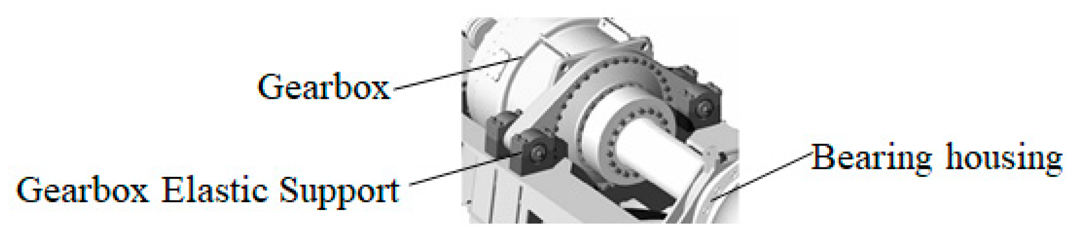
A gearbox elastic support is mainly used in three-point support wind turbine systems and is typically installed in pairs within the support seats on both sides of the gearbox. It primarily bears the weight of the gearbox as well as various loads transmitted from the rotor. Featuring excellent vibration damping performance, it can effectively resist both radial and axial loads while providing a certain degree of displacement compensation. An installation schematic of the gearbox elastic support is shown in Figure 9.

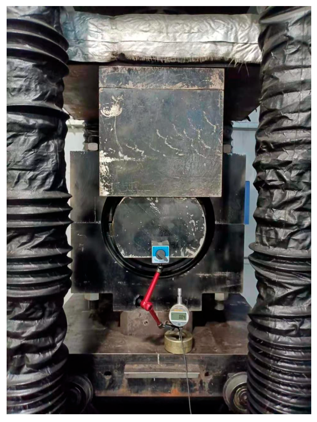
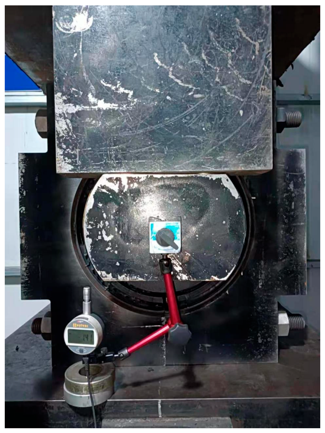
This study investigates the elastic support of a gearbox in a high-power wind turbine from a specific company, with physical tests performed to evaluate its bidirectional stiffness. The vertical and lateral forces acting on the gearbox elastic support are determined by actual operating conditions, both being 1650 kN.

A servo-hydraulic universal testing machine is employed to measure the directional deformation of the gearbox elastic support under varying load values, allowing for the calculation of the bidirectional static stiffness of the entire structure. The experimental setups for evaluating the vertical and lateral stiffness of the gearbox elastic support are shown in Figure 10 and Figure 11, respectively.

The static stiffness of the gearbox elastic support is calculated using the secant method, as follows:

$$K={\displaystyle \frac{F}{S_2-S_1}}$$

(17)

In this equation, $F$ is the measured load value, and $S_2$ is the measured directional displacement of the torque arm (transverse or vertical) under the load value.

$S_1$ is the directional displacement of the torque arm in the vertical direction under pre-compression, and the directional displacement of the torque arm in the lateral direction under pre-compression is 0.

To test the elastic support bidirectional stiffness of the gearbox and simulate the actual operating conditions, a vertical displacement of 10 mm is first applied to the elastic gearbox support, ensuring that the upper and lower supports of the elastic support are in close contact. Then, a load of 1650 kN is applied to the torsion arm of the gearbox elastic support in both the lateral and vertical directions. The vertical and lateral displacements of the torsion arm of the gearbox elastic support are measured to evaluate the stiffness.

3.1.1. Establishment of a 3D Model

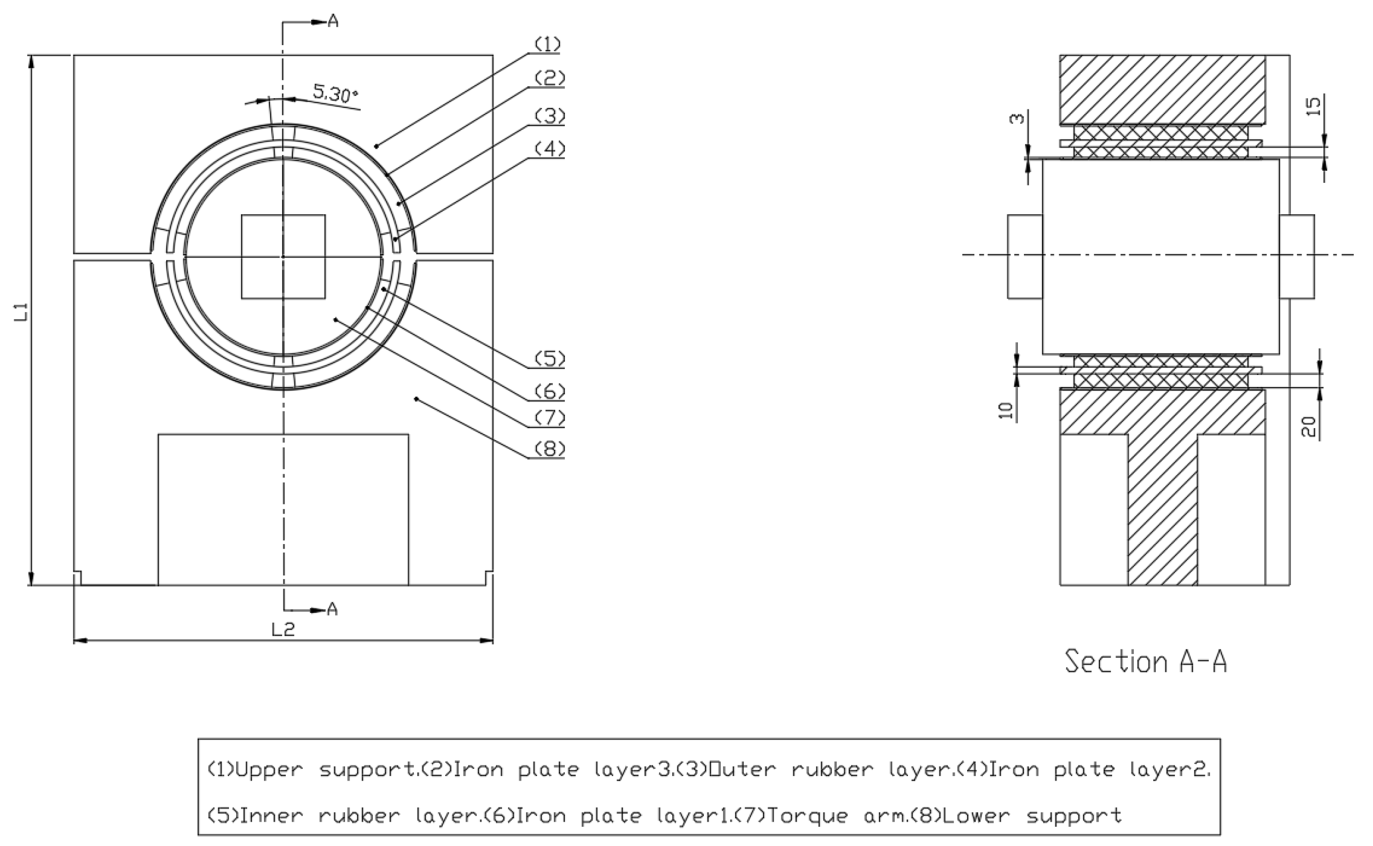
To perform simulation calculations, parametric modeling of the gearbox elastic support is required. A schematic diagram of the gearbox elastic support is shown below (see Figure 12). The metal–rubber composite structure consists of three layers of metal sheets, two layers of rubber, and upper and lower support seats. A metal sheet layer (Layer 1) is placed between the torque arm and the inner rubber layer, while a metal sheet layer (Layer 3) is positioned between the upper and lower support seats and the outer rubber layer. A metal sheet layer (Layer 2) is inserted between the inner and outer rubber layers. The metal layers are bonded to the rubber layers through vulcanization. The thicknesses of Layers 1 and 3 are the same.

Five parameters, namely the thickness of the inner iron sheet D1, the thickness of the inner rubber layer D2, the thickness of iron sheet layer 2 D3, the thickness of the outer rubber layer D4, and the rubber angle $\mathsf{\alpha }$ are selected as design parameters. According to industrial design requirements, the value ranges of these five design variables are as shown in

Table 1. Value ranges of design parameters.

Design Variables	${\mathit{D}}_1$/mm	${\mathit{D}}_2$/mm	${\mathit{D}}_3$/mm	${\mathit{D}}_4$/mm	$\mathsf{\alpha }$/(°)
Maximum value	4.5	16	11	21	8
Initial value	3	15	10	20	5.3
Minimum value	2	14	9	19	4

.

3.1.2. Rubber Material Parameters

The elastic support of the gearbox adopts a metal–rubber composite structure, in which the metal components are made of QT345 material. Its specific parameters are shown in the

Table 2. QT345 metal material parameters.

Material Property	Value
Density (kg·m−3)	7850
Young’s modulus (GPa)	206
Poisson’s ratio	0.28
Yield stress (MPa)	345
Allowable stress (MPa)	230

below. The rubber part uses natural rubber with a Shore hardness of 77. The elastic supports of gearboxes usually have higher requirements for service life during use. Compared with modified rubber, natural rubber has a higher strength and excellent fatigue resistance. Therefore, in the wind power generation industry, natural rubber is the most widely used elastic material.

The yield stress is ${\sigma }_b$ = 345 Mpa, the allowable stress is [$\sigma$] = ${\sigma }_b$/n, and n is the security coefficient. The safety factor is set to 1.5 (the safety factor for QT345 is between 1.5 and 2.0), and allowable stress [$\sigma$] = 230 MPa.

Natural rubber plays a critical role in the stiffness and vibration-damping performance of the gearbox elastic support structure. However, due to its highly nonlinear behavior and large deformation characteristics, the constitutive modeling of rubber is inherently complex, posing significant challenges for the design and engineering application of rubber components [27]. Numerous studies have been conducted to address the selection of appropriate constitutive models for rubber materials [28]. Currently, researchers commonly adopt phenomenological models that treat rubber as a continuous medium, describing its mechanical behavior by constructing a strain energy density function. The general form of the strain energy density function for rubber is expressed as:

$$U=f\left(I_1-3,I_2-3\right)+g\left(J-1\right)$$

(18)

The above equation is expanded using a Taylor series.

$$U=\sum _{i+j=1}^N{C}_{ij}{\left(I_1-3\right)}^i{\left(I_2-3\right)}^j+\sum _{i=1}^N{\displaystyle \frac{1}{D_i}}{\left(J-1\right)}^{2i}$$

(19)

In the equation, $f$ is the deviatoric (shear) strain energy potential;

$g$ is the volumetric (dilatational) strain energy potential;

$N$ is the degree of the polynomial;

$C_{ij}$, $D_i$ are the shear and compressibility parameters of the material, respectively, and are obtained from rubber material experiments. Generally, it is common to deal with rubber materials for most works as incompressible and set $D_i$ to zero. So, a lot of focus on hyperelastic models is awarded to the deviatoric strain potential [29].

$I_1,I_2$ are the first and second strain invariants.

$J$ is the volume ratio after deformation to before deformation. For incompressible materials $J$ = 1 [30].

For Equation (19), if N = 1 and the polynomial model includes only first-order terms, then the strain energy function reduces to the Mooney–Rivlin constitutive model expression:

$$U=C_{10}\left(I_1-3\right)+C_{01}\left(I_2-3\right)$$

(20)

For Equation (19), if N = 1 with i = 1 and j = 0, then the strain energy function reduces to the Neo-Hookean constitutive model expression:

$$U=C_{10}\left(I_1-3\right)$$

(21)

For Equation (19), if N = 3 and i ≠ 0, j = 0, then the strain energy function reduces to the Yeoh constitutive model expression:

$$U=\sum _{i=1}^3{C}_{i0}{\left(I_1-3\right)}^i$$

(22)

The Mooney–Rivlin model features a relatively simple strain energy function and can accurately capture the mechanical behavior of rubber materials under small to moderate deformations. However, it falls short in describing material hardening during large deformations. Similar to the Mooney–Rivlin model, the Neo-Hookean model is also suitable for small to moderate deformation scenarios but exhibits limited adaptability under large deformation conditions. In contrast, the Yeoh model offers higher accuracy in characterizing the mechanical properties of rubber materials, particularly as it provides a more precise and stable representation of the stress–strain relationship under large deformations. Given that the gearbox elastic support undergoes significant strain under normal operating conditions, in this study, the Yeoh model is adopted as the constitutive model for the rubber material, and it is applied in the subsequent numerical simulation analyses.

To ensure the accuracy of the model parameters, in this study, a natural rubber compression sample with a Shore hardness of 77 is used as an example, with the true stress–strain data of the sample obtained through uniaxial compression tests. Data fitting for the constitutive model is carried out using ANSYS 2022 simulation software. These parameters not only accurately reflect the mechanical properties of the rubber material under large strain conditions but also provide a solid foundation for subsequent simulation calculations, which helps improve the predictive accuracy of the model and enhances its reliability in practical engineering applications. The rubber specimen, experimental equipment, and rubber model parameters are detailed below, as shown in Figure 13 and

Table 3. Rubber material parameters.

Rubber Hardness	${\mathbf{C}}_{10}$	${\mathbf{C}}_{20}$	${\mathbf{C}}_{30}$	${\mathbf{D}}_1$	${\mathbf{D}}_2$	${\mathbf{D}}_3$
77	5.5995 × 105	3.6724 × 105	−15,756	0	0	0

.

3.1.3. Finite Element Analysis of Gearbox Elastic Support

Using the statics module in ANSYS Workbench, a force analysis of the gearbox elastic support under-rated working conditions is carried out. In order to simulate the actual working conditions, first, a vertical displacement of 10 mm is applied to the upper support of the gearbox elastic support to ensure that the upper support makes contact with the lower support. The upper and lower supports are set as frictional contact, and the friction coefficient is set to 0.2. Second, the mesh is divided. The sweeping method is adopted for the rubber element of the gearbox elastic support with a mesh size of 14 mm. A tetrahedral mesh is used for both the iron sheet and the upper and lower support pedestals. The mesh size of the upper and lower support pedestals is 35 mm, and that of the iron sheet is 15 mm. Finally, the bottom of the support seat under the elastic support of the gearbox is set as a fixed constraint, and a 1650 kN load is applied to the upper and side surfaces of the torsion arm of the elastic support for simulation. The simulation results are shown below.

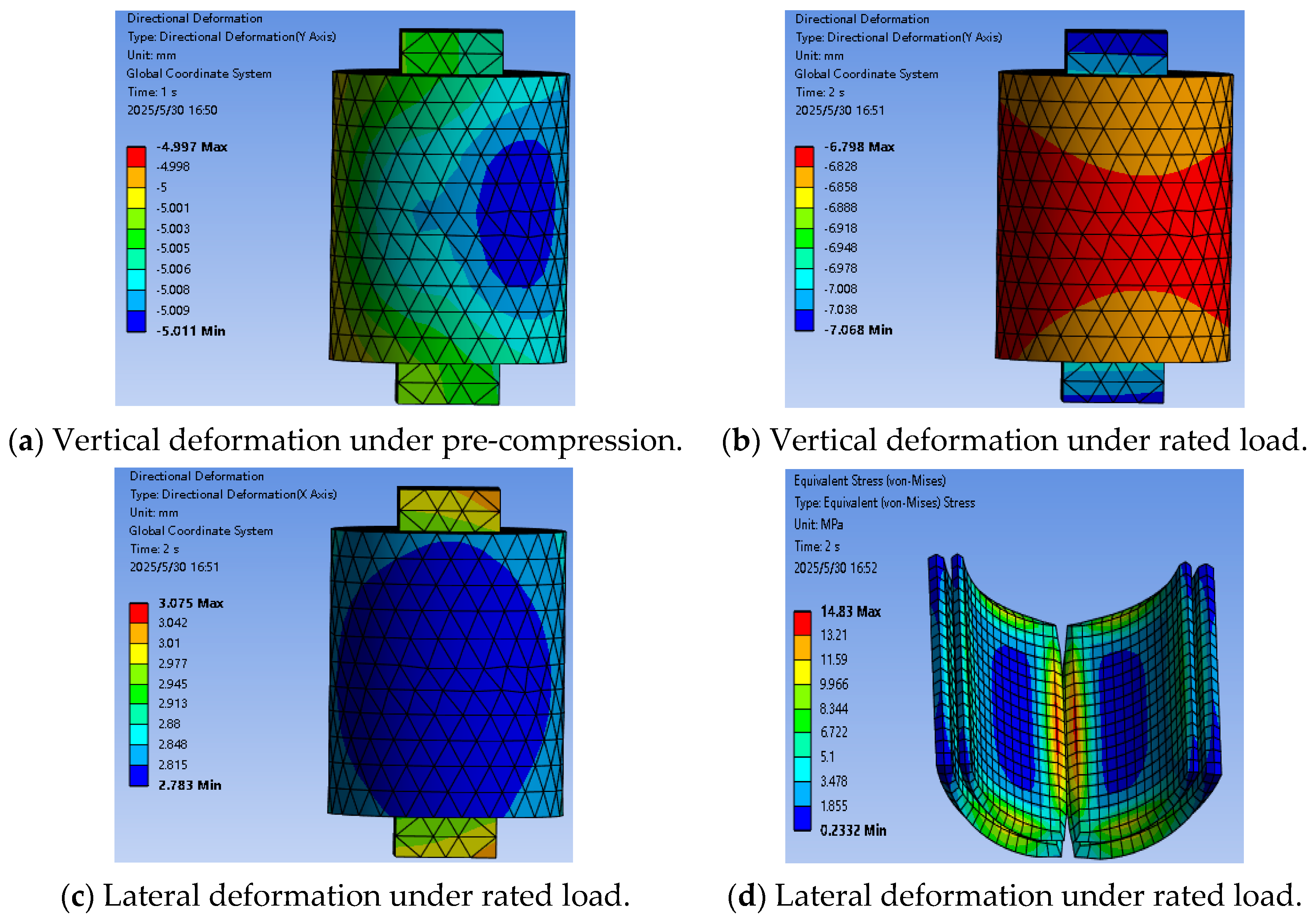
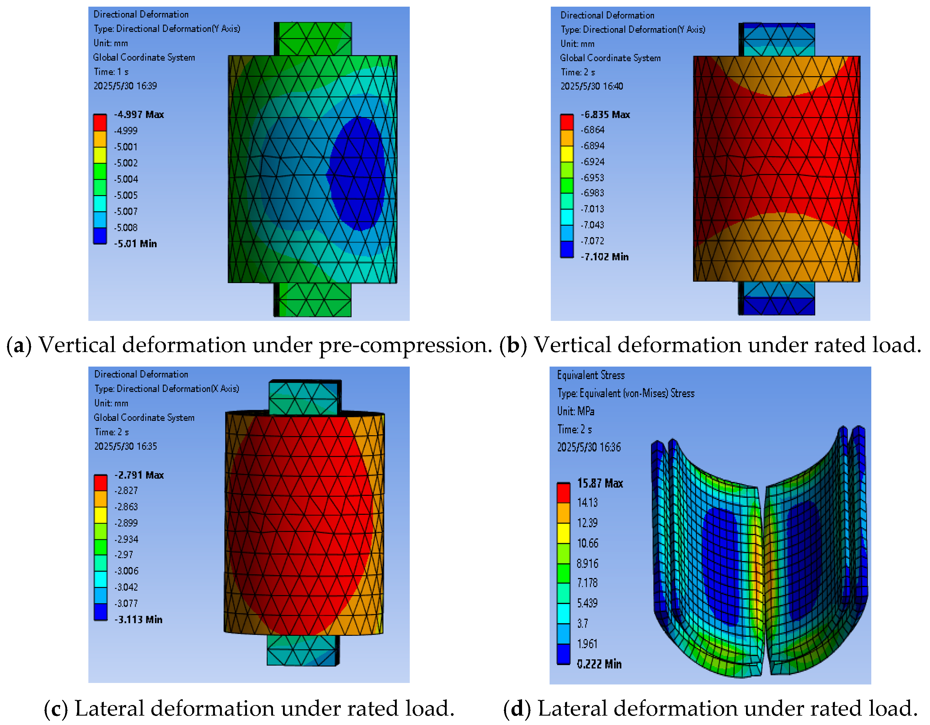
Figure 14 presents the finite element simulation results of the gearbox elastic support under different working conditions, allowing for an evaluation of its stiffness performance and the equivalent stress distribution of the rubber components. Figure 14a illustrates the vertical deformation of the torque arm under pre-compression conditions, Figure 14b and Figure 14c show the deformation of the torque arm in the vertical and horizontal directions, respectively, under a rated load of 1650 kN, and Figure 14d presents the equivalent stress contour of the rubber component under the same load. In the simulation, the average vertical deformation of the torque arm of the elastic support under a rated load is used as the displacement to evaluate the vertical stiffness of the elastic support, while the average horizontal deformation of the torque arm under a rated load is used to evaluate the horizontal stiffness. According to the stiffness calculation formula, the vertical static stiffness obtained from the simulation is 816.83 kN/mm, with an error of 8.5% compared to the physical experimental results; the horizontal static stiffness is 546.35 kN/mm, with an error of 8.7%. The discrepancies between the finite element analysis outcomes and the empirical experimental data are below 10%, effectively confirming the simulation’s reliability.

3.1.4. Experimental Design

An experimental design is employed using the optimal Latin hypercube sampling method combined with a finite element analysis. Input variables are sampled within the specified parameter range, resulting in a total of 500 samples. These 500 samples are then used as design points for a simulation analysis with ANSYS Workbench 2022 to generate a dataset. The hardness of the rubber material in data set 1 is 77, and that of the rubber material in dataset 2 is 75. The two datasets with different rubber hardness values are presented in

Table 4. Data set with hardness of 77.

Serial Number	Design Variables					Performance Indicators
	${\mathbf{D}}_1$/ mm	${\mathbf{D}}_2$/ mm	${\mathbf{D}}_3$/ mm	${\mathbf{D}}_4$/ mm	$\mathsf{\alpha }$/ (°)	${\mathbf{K}}_1$/ KN/mm	$\mathsf{\sigma }/$ Mpa	${\mathbf{K}}_2$/ KN/mm	$\mathbf{M}$/ Kg
1	2.84	14.38	10.13	20.85	4.75	1145.81	18.89	739.91	873.38
2	2.74	14.70	10.48	20.36	7.43	1198.61	18.96	774.64	873.75
3	2.56	15.45	10.96	19.54	4.56	1289.17	18.46	816.84	874.01
…	…	…	…	…	…	…	…	…	…
499	3.38	15.11	9.32	19.85	6.71	1213.23	17.43	881.46	874.07
500	3.23	14.61	9.97	20.03	6.57	1259.52	17.18	812.88	874.72

and

Table 5. Dataset with hardness of 75.

Serial Number	Design Variables					Performance Indicators
	${\mathbf{D}}_1$/ mm	${\mathbf{D}}_2$/ mm	${\mathbf{D}}_3$/ mm	${\mathbf{D}}_4$/ mm	$\mathsf{\alpha }$/ (°)	${\mathbf{K}}_1$/ KN/mm	$\mathsf{\sigma }/$ Mpa	${\mathbf{K}}_2$/ KN/mm	$\mathbf{M}$/ Kg
1	4.02	14.86	9.01	19.14	6.13	1025.45	14.06	697.21	876.01
2	2.22	15.98	10.74	19.86	6.27	905.78	15.17	627.35	872.23
3	2.55	15.45	10.93	19.54	4.55	961.47	14.14	652.01	874.01
…	…	…	…	…	…	…	…	…	…
499	2.42	15.86	10.56	19.78	7.39	921.77	14.33	627.92	872.68
500	3.86	14.00	9.70	19.61	7.76	1045.02	13.81	713.93	876.80

, respectively.

3.2. Data Preprocessing

In this section, two datasets generated using the optimal Latin hypercube sampling method and ANSYS Workbench simulation are processed to meet the needs of multi-task learning model training. The data consist of five design variables as inputs and four performance metrics as outputs, which are used for both model training and evaluation.

Before training the neural network, the data need to be normalized. The purpose of data normalization is to adjust features with different scales or units to the same range in order to improve the efficiency and stability of model training. This helps to prevent certain features from disproportionately affecting the model due to their large or small value ranges, thus accelerating the convergence of the algorithm and enhancing the model’s performance. Normalization is especially important when dealing with features that have different units or value ranges, as it helps to ensure a more balanced contribution from all features to the model. The formula used for data normalization is as follows:

$$X_n={\displaystyle \frac{{X-X}_{min}}{X_{max}-X_{min}}}$$

(23)

In the equation:

$X_n$ represents the normalized values;

$X$ represents raw data;

$X_{max}$ is the maximum value of the data;

$X_{min}$ is the minimum value of the data.

To evaluate the model performance in this study, the mean squared error (MSE) and the coefficient of determination (R²) are employed to assess the predictive results of the network model. The formulas for the MSE and R² are as follows.

$$MSE={\displaystyle \frac{1}{N_P}}\sum _{i=1}^{N_P}{\left(y_i-{\widehat{y}}_i\right)}^2$$

(24)

$$R-squared={\displaystyle \frac{{\displaystyle {\sum }_{i=1}^{N_P}}{\left(\widehat{y}-y_{mean}\right)}^2}{{\displaystyle {\sum }_{i=1}^{N_P}}{\left(y_i-{\widehat{y}}_{mean}\right)}^2}}$$

(25)

Here: ${\widehat{y}}_i$ is the predicted value, $y_i$ is the true value, $y_{mean}$ is the average of the true values, $N_P$ is the sample size.

3.3. Model Comparison Experiment Based on Multi-Task Learning

The multi-task learning model is implemented based on the programming software Pycharm 2023. The model’s input consists of five structural design parameters of the gearbox’s elastic support, while the output includes four structural performance parameters of the elastic support. Specifically, Task 1 is the vertical stiffness of the elastic support, Task 2 is the maximum equivalent stress of the elastic support, Task 3 is the lateral stiffness of the elastic support, and Task 4 is the mass of the elastic support.

The multi-task learning PLE and PLE-LSTM frameworks are both composed of two layers of CGC neural networks. The lower CGC network consists of five expert networks and five gating networks, while the upper CGC neural network is made up of five expert networks, four gating networks, and four tower networks. The upper expert networks receive inputs from the lower gating networks and pass the outputs to the upper gating networks. After processing the received data, the gating networks forward the results to the tower networks, which ultimately process the data and generate predictive outputs. In the multi-task learning PLE framework, both the expert and tower networks are fully connected neural networks, with 64 and 32 neurons in the hidden layers, respectively. For the PLE-LSTM learning framework, the tower networks are replaced by LSTM networks. All other settings remain consistent with those of the PLE framework.

For comparison, MLP and MMOE are introduced as control groups in this experiment. The MLP has a simple structure and is a typical hard parameter-sharing model in multi-task learning. In this experiment, the MLP structure is configured with three hidden layers containing 13, 27, and 13 neurons. The activation function used is ReLU. The MMOE framework consists of five expert networks, four tower networks, and four gating units. The expert networks are fully connected neural networks with two hidden layers containing 64 and 32 neurons

The MLP, PLE, MMOE, and PLE-LSTM network frameworks are used to train the data. The mean square error (MSE) is used as a loss function for each task. After training, the determination coefficients (R²) obtained for the four models on the verification set are shown in

Table 6. Coefficients of determination for multiple neural network models.

TASK	MLP		MMOE		PLE		PLE-LSTM
	77	75	77	75	77	75	77	75
Task 1	0.82	0.84	0.88	0.86	0.92	0.91	0.97	0.96
Task 2	0.76	0.74	0.82	0.81	0.88	0.87	0.95	0.94
Task 3	0.83	0.82	0.91	0.90	0.95	0.94	0.96	0.97
Task 4	0.92	0.91	0.97	0.96	0.97	0.97	0.99	0.99

.

The prediction accuracy pairs of the four tasks under different models are shown in Figure 15.

As shown in the above, PLE-LSTM, which is an improvement of the PLE framework, outperforms the other models in Tasks 1, 3, and 4. However, for the nonlinear features of Task 2, the prediction accuracy remains relatively low. Compared to the linear weighted approach used to optimize the loss function in the PLE-LSTM framework, in this study, dynamic loss weight allocation based on the GradNorm method is implemented, integrating the total loss function. Then, ablation experiments are carried out with other loss function optimization methods on the data set of mechanical properties of elastic support structures. After training, the predictive ability of the network model trained on the verification dataset using various methods is examined, as shown in

Table 7. Comparison experiment of multi-task loss function optimization methods.

TASK	UW		DWA		PCGRD		GradNorm
	MSE	${\mathit{R}}^2$	MSE	${\mathit{R}}^2$	MSE	${\mathit{R}}^2$	MSE	${\mathit{R}}^2$
Task 1	1.4 × 10−3	0.96	4.6 × 10−3	0.82	1.8 × 10−3	0.95	8.2 × 10−4	0.97
Task 2	3.8 × 10−3	0.86	1.8 × 10−2	0.69	5.7 × 10−3	0.82	9.2 × 10−4	0.95
Task 3	1.5 × 10−3	0.94	5.5 × 10−3	0.80	3.5 × 10−3	0.96	2.9 × 10−3	0.96
Task 4	5.2 × 10−4	0.99	6.9 × 10−3	0.90	2.4 × 10−4	0.99	9.8 × 10−5	0.99

.

Under the same PLE-LSTM network architecture and parameter configuration conditions, the loss function optimization strategy proposed in this study is clearly superior to the other methods. As shown in Figure 16, the optimized loss function exhibits a faster convergence rate during training, with the loss value decreasing rapidly, allowing the model to learn more efficiently. Additionally, optimizing the loss function results in a significant reduction in the overall loss value, greatly improving model performance, as reflected by smaller errors. Furthermore, the loss curve of the optimized function is smoother, with less fluctuation, indicating improved stability during the training process. In contrast, the unoptimized loss function curve shows substantial fluctuations. Finally, the optimized loss function enhances the model’s generalization ability, effectively preventing overfitting or underfitting. This ensures that the model continues to perform well when handling new data.

3.4. Method Validation

As shown in previous comparisons conducted by a particular company, the discrepancies between the physical and simulation experimental results are relatively small, indicating that simulations can effectively reflect the actual performance. In this study, the neural network prediction results are also compared with the simulation results to verify the feasibility of the proposed method. The comparison between the neural network predictions and the simulation results is shown in

Table 8. Comparison of neural network prediction results with simulation results.

	${\mathbf{K}}_1$/ KN/mm	$\mathsf{\sigma }/$ Mpa	${\mathbf{K}}_2$/ KN/mm	$\mathbf{M}$/ Kg
Neural network prediction results	842.73	17.03	603.92	874.16
Simulation results	877.66	15.87	574.92	873.90

.

As shown in Table 8 and Figure 17, the prediction errors between the neural network and simulation results for all four tasks are within 8%, fully demonstrating the reliability and effectiveness of the proposed method in performance prediction.

4. Conclusions

This study employs the multi-task learning (PLE) neural network framework, coupled with a dynamic weighting loss function optimization technique, to conduct multi-objective predictions of the mechanical performance indicators for the gearbox elastic support structure of wind turbine systems.

First, this study combines simulation experiments with the optimal Latin hypercube sampling method to generate the dataset required for the neural network. The reliability of the simulation results is validated through a stiffness experiment. The dataset generated using this method effectively avoids the high costs associated with physical experiments, providing reliable data support for the subsequent training of the network model.

Next, it is found that the improved PLE LSTM model based on the multi-task learning PLE network framework can better deal with the nonlinear characteristics of the rubber material in gearbox elastic support. The GradNorm loss function optimization method can dynamically adjust the weight of each task, thus effectively avoiding overfitting problems and unbalanced multi-task loss reduction.

Finally, through ablation experiments on various datasets, it is verified that the PLE-LSTM network architecture introduced in this research surpasses alternative multi-task learning frameworks in modeling the performance metrics of the gearbox elastic support structure. Moreover, the loss optimization strategy utilized herein exhibits exceptional effectiveness in tackling issues of early convergence and uneven loss reduction compared to other optimization approaches.

In conclusion, the method proposed in this study provides a reliable and economical alternative to traditional physical tests of the gearbox elastic support structure. By utilizing simulation experiments and optimized neural network models, our method accurately predicts multi-objective performance at a lower experimental cost. This method provides practical value for the efficient development and optimization of damping elements in wind power systems.