GNSS-RTK-Based Navigation with Real-Time Obstacle Avoidance for Low-Speed Micro Electric Vehicles

Abstract

Autonomous navigation for micro electric vehicles (micro EVs) operating in semi-structured environments—such as university campuses and industrial parks—requires solutions that are cost-effective, low in complexity, and robust. Traditional autonomous systems often rely on high-definition maps, multi-sensor fusion, or vision-based SLAM, which demand expensive sensors and high computational power. These approaches are often impractical for micro EVs with limited onboard resources. To address this gap, a real-world autonomous navigation system is presented, combining RTK-GNSS and 2D LiDAR with a real-time trajectory scoring algorithm. This configuration enables accurate path following and obstacle avoidance without relying on complex mapping or multi-sensor fusion. This study presents the development and experimental validation of a low-speed autonomous navigation system for a micro electric vehicle based on GNSS-RTK localization and real-time obstacle avoidance. The research achieved the following three primary objectives: (1) the development of a low-level control system for steering, acceleration, and braking; (2) the design of a high-level navigation controller for autonomous path following using GNSS data; and (3) the implementation of real-time obstacle avoidance capabilities. The system employs a scored predicted trajectory algorithm that simultaneously optimizes path-following accuracy and obstacle evasion. A Toyota COMS micro EV was modified for autonomous operation and tested on a closed-loop campus track. Experimental results demonstrated an average lateral deviation of 0.07 m at 10 km/h and 0.12 m at 15 km/h, with heading deviations of approximately 3° and 4°, respectively. Obstacle avoidance tests showed safe maneuvering with a minimum clearance of 1.2 m from obstacles, as configured. The system proved robust against minor GNSS signal degradation, maintaining precise navigation without reliance on complex map building or inertial sensing. The results confirm that GNSS-RTK-based navigation combined with minimal sensing provides an effective and practical solution for autonomous driving in semi-structured environments.

1. Introduction

The global push toward sustainable transportation has brought micro electric vehicles (micro EVs) to the forefront of smart mobility solutions. Designed for short-range, low-emission travel, these compact vehicles have become increasingly popular for urban commuting, university campus transit, and operations within industrial facilities [1]. Their small size, energy efficiency, and low environmental impact make them particularly suitable for semi-structured environments, where large vehicles may be impractical. As cities strive to reduce carbon footprints and implement green transportation policies, micro EVs offer a promising path forward [2,3].

One of the key technological advancements to further enhance micro EV utility is autonomous navigation. Equipping these vehicles with the ability to self-navigate not only reduces human intervention but also opens up opportunities for low-cost, flexible transit services. However, autonomous driving demands precise localization and robust obstacle avoidance capabilities, especially in environments where Global Navigation Satellite System (GNSS) signals may be intermittently degraded or obstructed by buildings and trees [4].

Accurate localization is the backbone of any autonomous vehicle system. Traditional GNSS provides meter-level accuracy, which is insufficient for precise navigation in narrow or constrained environments [5]. To address this, real-time kinematic (RTK) GNSS has been widely adopted. RTK enhances GNSS accuracy to the centimeter level by utilizing real-time correction data from a nearby base station [6]. Studies show that RTK-GNSS can maintain reliable positioning in semi-open areas, making it highly suitable for micro EV navigation on campuses and similar environments [7,8].

Several works have assessed the performance of low-cost RTK modules for autonomous driving [9]. For instance, the u-blox ZED-F9P module is a multi-band GNSS receiver that delivers centimeter-level accuracy in seconds, supporting the concurrent reception of all major GNSS constellations [10]. Although GNSS-RTK alone is sometimes affected by signal blockage, its integration with lightweight map-free approaches makes it a practical choice for micro EVs that lack the onboard computation power for multi-sensor fusion [4,11]. Researchers have also explored the fusion of GNSS with other sensors, such as inertial measurement units (IMUs) and light detection and ranging (LiDAR), but the tradeoff often involves increased complexity and cost [5,12].

Equally important as localization is the vehicle’s ability to avoid static and dynamic obstacles. Autonomous micro EVs must respond to unexpected hazards, such as pedestrians, parked vehicles, and construction barriers. Classical methods, like the dynamic window approach (DWA) [13], vector field histogram (VFH) [14], and artificial potential field (APF) [15], have been widely adopted in mobile robot navigation. These techniques use real-time sensor data to evaluate possible paths and select a collision-free direction.

DWA, for example, considers the kinematic constraints of the vehicle to generate a set of feasible trajectories and selects the best one based on a scoring function that balances progress toward the goal and safety [13]. VFH and APF, while computationally efficient, may struggle with narrow passages or local minima. Thus, scoring-based trajectory selection methods have gained traction, as they offer a balance between safety and control performance [16].

Recent work has explored heuristic scoring approaches, where paths are evaluated based on criteria such as heading deviation, lateral deviation, and minimum distance to obstacles [17]. These methods, when paired with 2D LiDAR and RTK-GNSS, can deliver real-time obstacle avoidance with minimal hardware requirements [18].

Advancements in machine learning have further enhanced obstacle avoidance capabilities. Deep reinforcement learning (DRL), for instance, enables vehicles to learn optimal avoidance strategies through interaction with the environment. DRL-based models can adapt to complex and dynamic scenarios, improving safety and efficiency [19]. Additionally, attention mechanisms in neural networks have been applied to optimize path planning and obstacle avoidance, allowing vehicles to focus on relevant environmental features and make informed navigation decisions [20].

Recent studies have also investigated the integration of RTK-GNSS with advanced learning and fusion-based techniques. For example, the authors of [21] proposed a robot navigation system that combines RTK-GNSS for path following with deep learning-based obstacle avoidance. Similarly, the authors of [22] demonstrated high-precision localization for railway inspection using a multi-sensor fusion framework involving RTK-GNSS, IMU, odometry, and laser sensing. These systems, while achieving excellent performance, often require complex hardware setups and significant computational resources.

Furthermore, the authors of [23] addressed the challenges of deploying time-sensitive services in connected and automated vehicles, highlighting the trade-offs between performance and resource constraints. These studies underscore the gap between high-accuracy, resource-intensive systems and practical deployment scenarios for micro EVs. In contrast, this study focuses on a lightweight and cost-effective navigation system optimized for semi-structured environments.

Semi-structured environments, such as university campuses or industrial parks, present unique challenges and opportunities for autonomous systems. These areas are often characterized by partially structured layouts, predictable traffic flows, and intermittent pedestrian activity [3,24]. For such settings, micro EVs are ideal due to their agility and lower speeds (typically 10–15 km/h).

In these contexts, high-definition maps and full 3D LiDAR systems are often unnecessary or impractical. Instead, cost-effective systems that combine RTK-GNSS with real-time obstacle avoidance provide a feasible solution [25]. These systems can maintain path-following accuracy within 10 cm, while successfully navigating around dynamic and static obstacles [18,26].

However, many prior studies on autonomous driving have focused on achieving high accuracy through complex multi-sensor fusion—such as vision-based SLAM or 3D LiDAR—which typically require expensive sensors and high-performance computing platforms. Such solutions may be infeasible for micro electric vehicles operating in structured or semi-structured environments, such as university campuses or industrial areas, where limited onboard processing power, budget constraints, and the absence of full 3D maps necessitate simpler, scalable alternatives.

To address this gap, we propose a GNSS-RTK-based navigation system with minimal sensor requirements, emphasizing low system complexity and practical deployment feasibility. This study addresses these needs by implementing and validating a real-world autonomous navigation system based on GNSS-RTK and a real-time scored predicted trajectory algorithm. The system is designed specifically for micro electric vehicles and has been tested in a real university campus environment using a Toyota COMS platform [18].

The main contributions of this work are as follows:

• Integrated system combining GNSS-RTK and 2D LiDAR for localization and obstacle avoidance, suitable for deployment in micro EVs.
• The development of a trajectory scoring algorithm that evaluates candidate paths using heading error, lateral deviation, and collision distance.
• Real-world validation in a semi-structured environment, demonstrating safe and accurate path following at low speeds.

This research helps close the gap between academic research and practical deployment of micro EV autonomy, contributing toward sustainable, intelligent transportation solutions.

2. System Architecture and Integration

2.1. Micro EV Platform: Toyota COMS and Hardware Modification

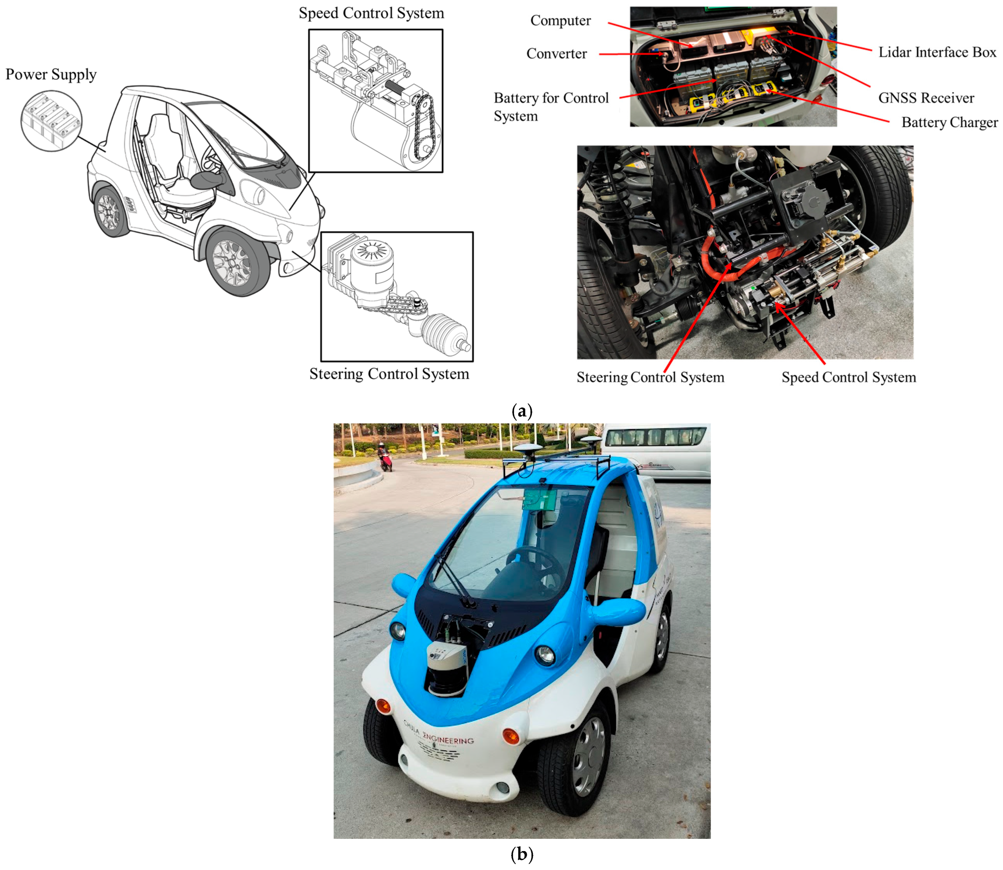
The experimental platform utilized in this study is the Toyota COMS ZAD-TAK30-DS (Toyota Auto Body Co., Ltd., Kariya, Japan), an ultra-compact, single-seat electric vehicle powered by a permanent magnet synchronous motor. With a curb weight of 420 kg and a total length of 2395 mm, the COMS is designed for low-speed urban mobility at typical speeds of 10–15 km/h, making it well-suited for semi-structured environments, such as university campuses [27]. To enable autonomous operation, the vehicle’s conventional controls were extensively modified at the low-level hardware layer. Custom drive-by-wire systems were integrated for steering, acceleration, and braking, while additional sensors and a dedicated power supply system were installed. These modifications not only enable full autonomous control but also preserve the ability for manual operation, ensuring safe testing and easy intervention when necessary. An overview of the modified vehicle is shown in Figure 1.

2.2. Steering Control System

A high-torque DC motor and gearbox assembly is attached to the steering column via a chain-drive (overall ~1:9.8 gear reduction). This actuator can turn the front wheels under computer control. A multi-turn potentiometer is mounted on the steering column to provide feedback from the steering angle. The steering motor driver is an H-bridge controlled by a microcontroller, with the drive voltage limited (~50% duty cycle) to prevent excessive torque for safety [27]. An emergency stop switch and a manual disconnect (circuit breaker) are integrated into the steering power circuit to immediately disable power assist if needed, ensuring the vehicle remains controllable in emergencies. Calibration tests were performed on the steering loop, and the controller gains were tuned so that a step input in the desired angle yields a prompt, critically damped response with minimal overshoot, suitable for precise maneuvers.

2.3. Brake Control System

The stock hydraulic brake line is modified to include a custom electro-hydraulic actuator in series. The added module incorporates dual master cylinders and an electric drive that can pressurize the front and rear brake circuits. In normal conditions, the original brake pedal and master cylinder function are unhindered; during autonomous mode, a lead screw-driven piston pushes fluid to apply the brakes. This in-line brake actuator design allows both the human driver and the autonomy system to generate braking pressure as needed, offering a redundant failsafe design. The brake actuator’s motor is powered at 24 V through an H-bridge driver and is current-limited (to ~75% max) to avoid overstressing the mechanism. Like the steering, the braking system was characterized and tuned—for example, ensuring that when a full brake command is issued, the response is smooth, and the vehicle decelerates at a controlled rate without oscillation.

2.4. Acceleration Control System

The electric accelerator (throttle) interface is achieved by intercepting the accelerator pedal position (APP) sensor signals. The COMS’s pedal has dual analog outputs (for redundancy) that feed the vehicle’s motor controller via the ECU. A custom circuit with a dual 12-bit digital-to-analog converter (DAC) and failsafe relays allows the autonomy system to over-ride these signals. In autonomous mode, the microcontroller-generated analog voltages replace the pedal outputs, commanding motor torque directly; otherwise, the relays default to pass through the driver’s pedal signals. This design permits seamless switching between manual and computer control of acceleration. The vehicle’s actual speed is read from the CAN bus and used in a closed-loop speed controller. The low-level speed controller uses a PID law that coordinates the throttle and brake; if the target speed is higher than current, the throttle DAC is engaged (with brake released), and if lower, the brake actuator is applied (with throttle zeroed). A small deadband around the target prevents oscillation by avoiding simultaneous throttle and brake commands. System response testing of the speed control showed that the vehicle can accelerate and decelerate to track speed setpoints with minimal steady-state error and no undue oscillations (e.g., a 0–30 km/h speed step was achieved with a smooth rise and negligible overshoot in the PID response).

Beyond the primary control modifications, additional electronic interfaces were integrated to support auxiliary functions, such as gear selection and turn indicators. Relay-based circuits allow the onboard computer to operate these controls during autonomous mode, while preserving manual operation by the driver. This design ensures that the micro EV can be fully controlled autonomously when needed yet easily switched back to manual control for safety or testing purposes.

2.5. GNSS-RTK and LiDAR Sensor Setup and Placement

For environmental perception and localization, the vehicle is equipped with a high-precision GNSS receiver and a 2D LiDAR. This sensor suite provides redundant, complementary data; the GNSS with real-time kinematic (RTK) correction provides accurate global position, while the LiDAR yields detailed local obstacle detection. All sensors are ruggedized and mounted to maximize coverage and accuracy in the campus setting. The sensor placement and integration were carefully chosen to support navigation among buildings and pedestrians, ensuring the platform maintains situational awareness and positioning reliability even in semi-structured or partially obstructed areas.

GNSS-RTK: The primary localization system employs a dual-antenna RTK-capable Global Navigation Satellite System (GNSS) receiver, providing centimeter-level positioning and real-time heading estimation [4]. Two antennas are mounted along the vehicle’s centerline to establish a known baseline, allowing orientation to be derived from phase measurements. Operating in differential mode with corrections from a fixed base station, the system consistently achieves centimeter-level accuracy even in the presence of a multipath from the surrounding structures. This high-accuracy localization enables reliable waypoint following in narrow campus pathways, validating the suitability of GNSS-RTK as the primary localization sensor for semi-structured environments.

LiDAR Obstacle Sensor: A SICK LMS511 planar LiDAR is mounted at the front of the vehicle to provide real-time obstacle detection and environment mapping. The sensor offers a wide field-of-view and sufficient range for outdoor navigation, with a 190° horizontal scan and robust operation under various weather conditions [28]. Positioned parallel to the ground, the LiDAR enables a top-down view of the path and surrounding areas, supporting the detection of both static and dynamic obstacles. Campus trials demonstrated reliable obstacle detection performance during both day and night, validating the LiDAR’s suitability for local situational awareness. Together with GNSS-RTK, the LiDAR forms a complementary perception system essential for safe autonomous driving in semi-structured environments.

2.6. Low-Level Control of Steering, Acceleration, and Braking

To translate high-level navigation decisions into vehicle motion, the platform employs dedicated low-level controllers for steering, throttle, and braking. These controllers were developed and calibrated to ensure smooth and stable vehicle response, which is critical for safety and comfort. Each actuator subsystem (steering, acceleration, braking) is governed by a closed-loop control law (PID-based), and extensive bench and field tests were conducted to tune these controllers’ gains and validate the system response. Figure 2 presents an overview of the control architecture, illustrating how sensor feedback and control commands are processed from the high-level computer down to the actuation of steering and brakes.

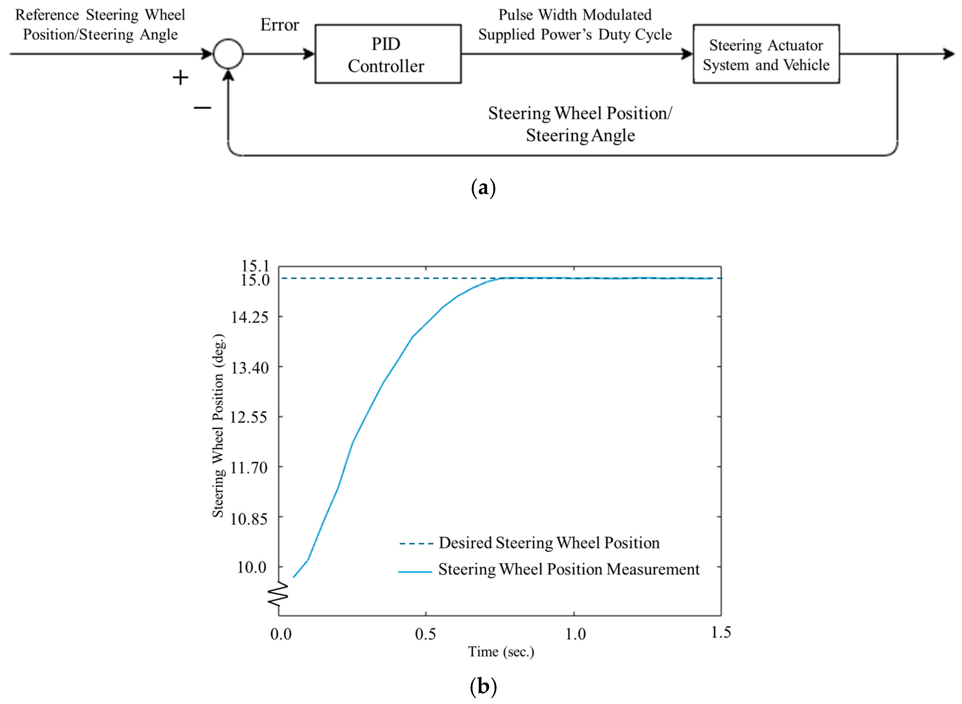
Steering Control: The steering subsystem receives the desired steering angles from the high-level path-following algorithm and adjusts the front wheel angle through a PID-controlled DC motor drive. In this context, the ‘steering angle’ refers to the commanded angle at the steering column actuator, while the ‘wheel angle’ denotes the actual deflection of the front wheels relative to the chassis. Due to the steering linkage ratio, the steering column rotates more than the wheels; however, the control system operates based on calibrated wheel angle measurements.

Wheel angle feedback is obtained via a 16-bit analog-to-digital converter (ADC) reading from a multi-turn potentiometer attached to the steering column. Calibration established that an ADC value of 880 corresponds to approximately −36°, 8800 corresponds to 0°, and 16,720 corresponds to +36°. This linear mapping enables straightforward conversion from raw ADC readings to physical wheel angles, ensuring consistent and accurate feedback across the entire steering range. A closed-loop proportional–integral–derivative (PID) controller is implemented in the microcontroller to ensure that the wheel angle accurately follows the commanded steering angle. The steering control system block diagram is shown in Figure 2a. The controller gains were tuned empirically to achieve a critically damped response with minimal overshoot ($K_p=280,K_i=150,K_d=10)$. Step response tests validated the system’s performance, showing that the steering can quickly and stably track sudden changes in angle, such as 10° and 15° step inputs, with rapid settling and negligible overshoot (Figure 2b).

To enhance prediction during path planning, a data-driven steering response model was developed. Instead of relying on a theoretical model, 729 steering response profiles were recorded empirically, each capturing the time-series wheel angle response to a step input across a grid of initial and target positions within the ±36° range. During operation, the high-level controller references the closest matching profile to predict the vehicle’s real-time steering behavior, improving prediction accuracy, while reducing computational load at the cost of additional memory usage.

Figure 2. Steering control system: (a) steering control system block diagram, (b) step response of a steering control system.

Figure 2. Steering control system: (a) steering control system block diagram, (b) step response of a steering control system.

To ensure safety, mechanical steering limits and actuator torque output were configured so that the system cannot exceed the vehicle’s normal steering range. An emergency stop (E-stop) circuit was also integrated directly into the steering motor power line, allowing immediate manual over-ride if any anomaly is detected during autonomous steering operation.

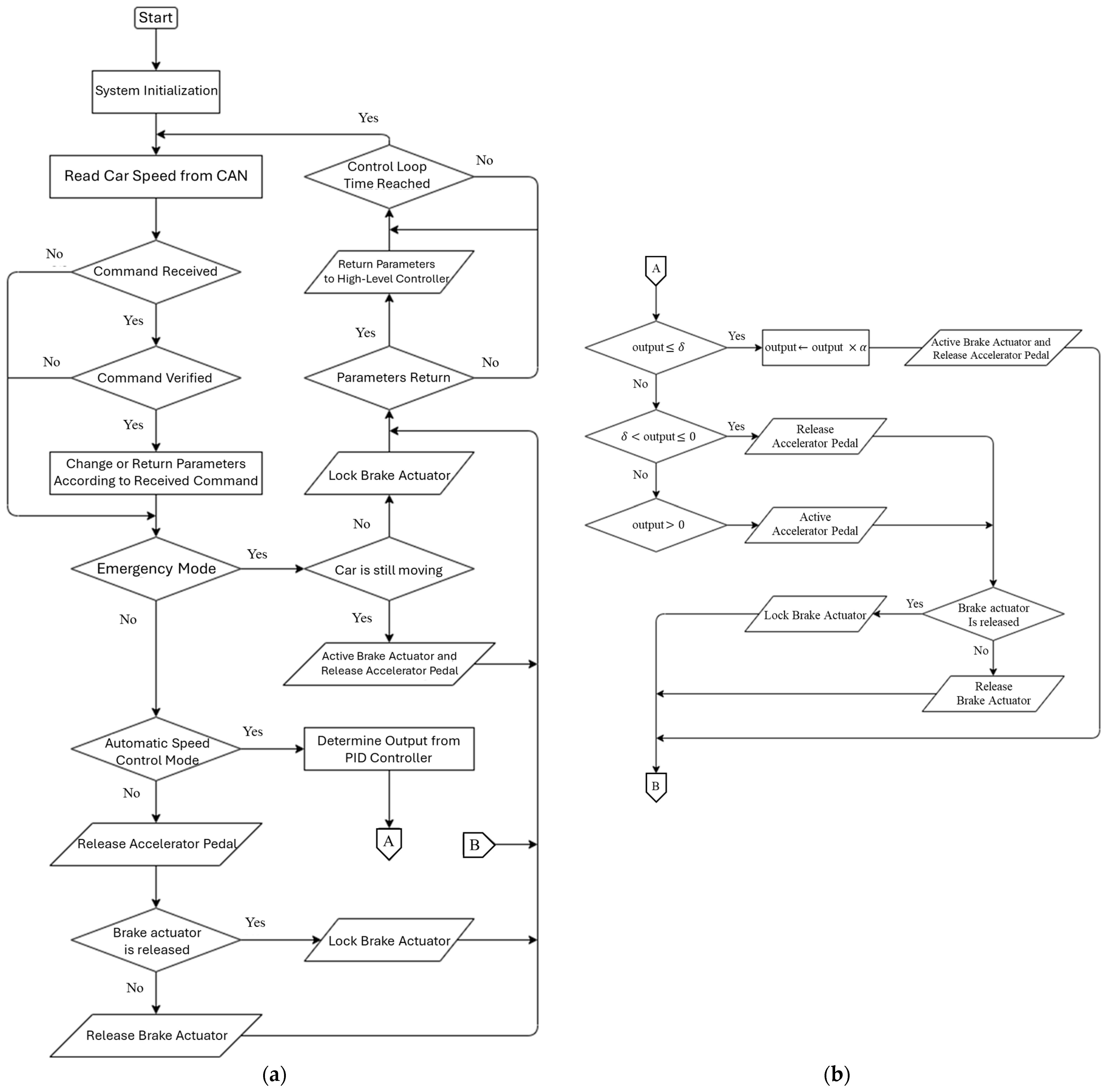
Acceleration and Braking Control: The low-level speed control system regulates the vehicle’s velocity based on the desired and current speeds. As shown in the system architecture diagram (Figure 3a), a PID controller operating at 200 Hz computes the control output, and the system commands either the throttle or the brake actuator accordingly. The throttle is controlled via a dual 12-bit DAC circuit that simulates accelerator pedal signals and sends torque commands to the motor controller (ECU) through the CAN bus, while braking is handled by an electro-hydraulic actuator driven by a DC motor with an H-bridge.

Speed is regulated in a closed-loop fashion using a PID controller operating on the error between the target speed (commanded by the high-level controller) and the measured vehicle speed. The actual vehicle speed is read from the car’s CAN-bus odometry data (with a resolution of 0.004 km/h) and is filtered (using a moving average of recent samples) to reduce sensor noise before feedback is used. The PID controller computes a control output at each cycle to minimize the speed error, and this output is then translated into appropriate throttle or brake commands. The low-level control loop runs at a high update rate of 5 ms (200 Hz), allowing it to react quickly to speed deviations and make fine adjustments for smooth control. This high frequency actuation ensures that any difference between desired and actual speed is corrected with minimal delay, preventing oscillations and providing stable speed tracking.

A discontinuous gain selection logic is employed to ensure that only one actuator (accelerator or brake) is active at any given time, mimicking cautious human driving behavior and avoiding conflicting commands. In essence, the PID output is fed into a piecewise function (implemented with a Heaviside step function and thresholds) that yields either an accelerator command or a brake command depending on the sign and magnitude of the control effort. If acceleration is required (PID output is positive), the system engages the throttle (simulating the accelerator pedal) and guarantees the brake remains fully released; conversely, if strong deceleration is required (PID output is sufficiently negative), the brake actuator is activated, while the throttle output is cut to zero. For small negative errors—indicating a need to slow down gently—neither actuator is driven (a ‘dormant’ interval), allowing the vehicle to coast or use its regenerative braking without applying the mechanical brake. This conditional logic (see Figure 3b) for the piecewise output mapping ensures a smooth transition between acceleration and braking; the accelerator is released before the brake is applied, preventing overlap. By introducing a deadband (dormant zone) and scaling the brake command with a constant gain to account for the brake actuator’s characteristics, the control system avoids jerky responses and reflects a conservative driving strategy. The result is a non-linear control output function that cleanly splits authority between the two actuators, as depicted in Figure 3b.

The effectiveness of this low-level speed control scheme is demonstrated by its step response performance. Figure 3c illustrates the vehicle’s response when commanded to accelerate from an initial speed of 3.6 km/h to a setpoint of 30.0 km/h. The tuned PID controller and gain scheduling ensure that the vehicle accelerates briskly to the target speed with a smooth, well-damped trajectory ($K_p=420,K_i=700,K_d=30,\alpha =2,\delta =1.2\times 10^5$). There is no excessive overshoot in speed; the controller transitions to braking (deceleration) if needed to prevent surpassing the setpoint and then maintains the desired speed with negligible steady-state error. The rise to 30 km/h is prompt and controlled, indicating that the 200 Hz low-level loop can adjust the throttle quickly, while invoking the brake only as necessary to settle at the commanded velocity. In steady-state cruising, the vehicle’s speed closely tracks the reference, validating that the low-level PID loop and actuator logic can achieve accurate and stable speed regulation. This high-frequency, single-actuator-at-a-time control approach, thus, provides fast acceleration, responsive deceleration, and reliable steady-state speed tracking in the autonomous micro EV platform.

Figure 3. Acceleration and braking control: (a) speed control system block diagram, (b) output of the discontinuous gain transfer function, (c) step response of a speed control system.

Figure 3. Acceleration and braking control: (a) speed control system block diagram, (b) output of the discontinuous gain transfer function, (c) step response of a speed control system.

2.7. Power Distribution Architecture for Autonomous Subsystems

A dedicated power distribution network was designed to reliably supply all added autonomous components (sensors, computers, and actuators) without overloading the COMS’s stock electrical system. Rather than drawing from the vehicle’s primary traction battery, the autonomous subsystems are powered by an independent battery pack. As shown in Figure 2b, the autonomous power system uses four 12 V, 45 Ah LiFePO₄ batteries arranged into two 24 V supply lines. One 24 V line is designated for high-demand actuators (the steering motor and brake motor), while the other 24 V line feeds the lower-power electronics. This includes the GNSS receiver, LiDAR scanner, onboard computer, and the microcontroller units. By separating the power domains in this way, voltage drop or noise from the steering/braking motors (which draw significant current during operation) does not disturb the sensitive sensors and computing hardware. Each supply line is equipped with appropriate regulators and protection (fuses and circuit breakers) to maintain stable voltages required by each device (for example, DC-DC converters step down 24 V to 12 V and 5 V for devices as needed). Both 24 V sub-batteries are charged via a single charging system; when the vehicle is plugged in, a charge controller isolates the batteries from the loads and charges all cells in balance. This power architecture ensures that the autonomous kit can run for extended periods; the 45 Ah capacity provides many hours of operation at typical load. Moreover, because the autonomous system’s power is independent, it can be fully powered on and tested without turning on the vehicle’s main motor, and it provides an extra layer of safety; any severe power fault in the autonomy circuit (e.g., short or brown-out) will not directly affect the vehicle’s traction power. In summary, the power distribution is robust and segregated, supplying clean power to sensors and actuators and thereby contributing to the overall reliability of the autonomous platform.

2.8. Overall System Architecture and Data Flow

The integration of all subsystems is structured through a layered control architecture that links sensors, processors, and actuators in real time (Figure 4). The design follows a sense–plan–act paradigm, separating high-level decision making from low-level actuation. An onboard Intel i7-based computer (Micro-Star International Co., Ltd., New Taipei City, Taiwan) runs the navigation software, including GNSS-based path following and obstacle avoidance, and communicates with a low-level microcontroller interfacing with the vehicle hardware.

At the perception layer, the GNSS-RTK receiver and LiDAR scanner continuously provide updated position, heading, and environment scans. GNSS data are converted into local Cartesian coordinates, while LiDAR point clouds are processed to detect obstacles and free space.

At the decision and planning layer, the autonomy software fuses sensor inputs to generate driving commands. Based on the current pose and a predefined waypoint route, the path-following module computes steering and speed commands, while the obstacle avoidance module adjusts trajectories if necessary. These high-level commands are transmitted via a robust serial link to the low-level controller. If commands are lost, the system safely stops the vehicle.

At the actuation layer, the low-level microcontroller executes the received commands. It controls steering via a PID loop and regulates speed by coordinating throttle and braking. Feedback from steering and CAN-bus speed sensors ensures precise execution, while status updates are sent back to the high-level computer for continuous monitoring.

This modular, hierarchical architecture proved highly reliable in campus trials, allowing the Toyota COMS to autonomously navigate dynamic semi-structured environments. The system’s design emphasizes robustness and safety; dual-antenna RTK ensures accurate localization, even near buildings [15], and independent actuator power protects against failures. Thus, the platform demonstrates practical viability for autonomous micro-mobility applications.

Figure 4. Low-level speed control software’s flowchart: (a) main flowchart, (b) sub flowchart.

Figure 4. Low-level speed control software’s flowchart: (a) main flowchart, (b) sub flowchart.

To clarify the software architecture and data flow of the proposed system, a workflow diagram is provided in Figure 5. The diagram illustrates how GNSS-RTK and LiDAR sensor inputs are processed through the real-time trajectory planning module, considering vehicle speed, and subsequently translated into low-level control commands for steering, throttle, and braking. This representation helps visualize the system’s internal coordination and the role of speed-aware planning in ensuring safe and accurate navigation.

3. Scored Predicted Trajectory Algorithm for Micro EV Path Planning

Micro EVs like the Toyota COMS face strict constraints that necessitate a carefully tailored navigation strategy. Unlike full-sized autonomous vehicles equipped with substantial processing power, micro EVs have limited computational and power resources. Additionally, these vehicles often operate in semi-structured environments, such as university campuses, where safe, real-time navigation around pedestrians and obstacles is essential. To address these challenges, a predictive trajectory approach was adopted to meet two critical needs: (1) real-time decision making—the system must determine steering actions quickly without relying on complex global planners or heavy optimizers that could compromise timing requirements; and (2) safe, smooth navigation—accurate path following and responsive obstacle avoidance must be achieved. The method predicts multiple candidate trajectories ahead of time and scores them at each planning cycle. This trajectory rollout approach enables the selection of the safest and most path-compliant maneuver. By simulating short-term vehicle motion, the system plans by preview rather than relying on reactive corrections. A data-driven predictive model is employed to reduce online computation, trading additional memory usage for faster, lightweight execution, which is well suited to the micro EV platform.

3.1. Trajectory Evaluation Metrics

Once a set of candidate trajectories is predicted, the algorithm evaluates each trajectory’s quality using the following three key metrics that reflect path-following accuracy and safety:

• Linear Deviation (Path Distance Error): This metric measures how far the predicted trajectory strays from the desired reference path in a lateral sense. The reference path can be defined by the line connecting the current position to the next waypoint or the preplanned route segment the vehicle should follow. For each point along the candidate trajectory, the shortest distance to the reference path is computed, and the linear deviation is typically quantified as the integral of this distance over the trajectory or the maximum deviation encountered. Effectively, this tells us if the vehicle would veer off course; a smaller value means the trajectory stays close to the intended path. If the micro EV is supposed to follow a campus walkway, for example, linear deviation indicates how well a candidate maneuver keeps it on that walkway centerline. The lateral distance error is denoted by $d_{lat}$.
• Angular Deviation (Heading Error): Even if a trajectory stays near the correct path, it may have the vehicle oriented incorrectly. Angular deviation measures the difference in heading (orientation) between the vehicle’s trajectory and the reference path’s direction. At each point along the trajectory, the vehicle’s heading is compared with the tangent direction of the reference path or the desired heading toward the waypoint. The error in orientation is accumulated (often using absolute values or squared error) to give a total heading discrepancy. This metric (denoted ${\theta }_{err}$) is zero for a trajectory perfectly aligned with the path and grows as the candidate path oscillates or approaches the waypoint at the wrong angle. Minimizing angular deviation is important for smooth path following; a large heading error at the waypoint could require abrupt corrections later.
• Collision Distance (Obstacle Proximity): This safety metric gauges how close the predicted trajectory comes to any detected obstacle. Using the latest 2D LiDAR scan, the system identifies obstacles as a set of points or a contour in the environment. For a given candidate trajectory, the algorithm checks each point along the trajectory against the obstacle map to find the minimum distance between the vehicle’s path and the nearest obstacle. If the vehicle is projected to pass very near an object (or hit it), this minimum distance will be small (or zero). Rather than using distance directly as a ‘cost’ (where larger values are better), a complementary cost is defined to penalize proximity. Specifically, a safe distance threshold $r_0$ (e.g., the vehicle’s radius plus a safety buffer) is set. If the minimum separation is below $r_0$, the trajectory is considered dangerous. In the implementation, any trajectory that violates the threshold is flagged, and later, in scoring, it will receive a very high penalty (effectively removing it from consideration). For distances above $r_0$, the collision metric can be defined as the inverse of the clearance or simply the negative of the minimum distance (so that larger clearances yield a better, lower ‘cost’). The metric $d_{obs}$ represents obstacle proximity, with lower values indicating riskier paths; trajectories violating the safety threshold are assigned infinite cost. This ensures that trajectories brushing too close to obstacles are strongly discouraged or outright eliminated.

By evaluating these three criteria, the algorithm captures the following essential trade-offs: path fidelity (stay on course), orientation (face the right direction), and safety margins (avoid obstacles). All metrics are computed over the finite prediction horizon (e.g., a few seconds or meters of travel). Notably, linear and angular deviations are calculated with respect to the next waypoint or path segment, which continuously updates as the vehicle moves, ensuring the vehicle gradually converges to each waypoint.

3.2. Path Scoring Mechanism

After computing the above metrics for a candidate trajectory, the algorithm combines them into a single score that represents the overall “goodness” of that trajectory. A weighted linear combination is used for this multi-objective evaluation. For trajectory $i$, we define a total score $S_i$ as:

$$S_i=w_d{D}_i+w_{\theta }{\mathsf{\Theta }}_i+w_c{C}_i$$

(1)

where $D_i$ is the linear deviation measure for trajectory $i$, ${\mathsf{\Theta }}_i$ is the angular deviation, and $C_i$ is the collision distance cost (after thresholding). The coefficients $w_d$,$w_{\theta }$, and $w_c$ are weights that determine the relative importance of each term. A lower score $S_i$ means a better trajectory (since smaller deviation and safer clearance yield lower weighted sums). The trajectory with the lowest score is selected for execution in the next time step.

The weight selection is crucial and was tuned empirically. In the implementation, we initially set $w_d$ and $w_{\theta }$ to comparable magnitudes (since both path deviation and heading error affect tracking quality) and set $w_c$ (obstacle term) to a value that strongly prioritizes safety. Safety is enforced via the threshold logic rather than relying purely on $w_c$. Any trajectory with a predicted obstacle distance below $r_0$ is assigned a massive penalty by setting $C_i=\infty$ for that trajectory, over-riding the linear weighted sum. Unsafe trajectories are assigned effectively infinite cost, ensuring hard safety constraints. For trajectories that are all safe (no imminent collision), the weights $w_d$:$w_{\theta }$ determine the bias between staying centered on the path versus aligning orientation. For instance, if the vehicle tends to cut corners, $w_d$ can be increased to penalize lateral offset more heavily. In practice, a balanced weighting (on the order of unity for each, adjusted by units) is effective, and $w_c$ is set large enough so that the planner prefers slightly more deviation if it significantly increases obstacle clearance. The weights remained fixed during the experiments, but they could be adjusted for different scenarios or even tuned automatically in future work. The scoring process evaluates multiple candidate paths at each planning step, selecting the one that minimizes the weighted sum of path deviation, heading error, and collision risk, while rejecting any paths that violate the safety buffer. For clarity, the scoring formula can be interpreted as a cost function being minimized; a concept analogous to optimization-based planners but implemented here in a discrete, heuristic manner.

3.3. Algorithmic Workflow and Pseudocode

The overall prediction–scoring–selection process is executed at each planning cycle (many times per second). It can be summarized in the following pseudocode:

1.

Input retrieval:

• Read current state: vehicle position $p$, heading $\theta$, and steering angle $\alpha$ from sensors.
• Obtain the current speed $v$ (assumed roughly constant during the short horizon).
• Fetch the next waypoint $W$ (or reference path segment) from the route plan.
• Obtain the latest obstacle scan (list of obstacle points $O$) within sensing range.

2.

Generate candidate steering commands:

• Define a discrete set of $M$ target steering angles {${\varphi }_1$, ${\varphi }_2$, $\dots$, ${\varphi }_M$} that the high-level controller could command.
• These typically span left to right limits (e.g., from −30° to +30°) in increments.
• The implementation uses 5° steps, corresponding to 27 profiles.

3.

For each candidate command ${\varphi }_i:$

a. Profile selection: Identify the prerecorded steering profile $\psi$ that best matches the current steering $\alpha$ and target ${\varphi }_i$. (If $\alpha$ exactly equals one of the profile’s initial angles, use that profile with final angle ${\varphi }_i$; otherwise, interpolate between the two profiles bracketing $\alpha$ to create a custom profile.)

b. Trajectory simulation: Starting from the current pose ($p$, $\theta$), simulate the vehicle’s motion forward in time using profile $\psi$ and speed $v$. At each time step $\mathsf{\Delta }t$, update:

$$\begin{gathered} x_{k+1}=x_k+v\mathrm{c}\mathrm{o}\mathrm{s}\left({\theta }_k\right)\mathsf{\Delta }t \\ {y}_{k+1}=y_k+v\mathrm{s}\mathrm{i}\mathrm{n}\left({\theta }_k\right)\mathsf{\Delta }t \\ {\theta }_{k+1}={\theta }_k+{\displaystyle \frac{vtan\left({\delta }_k\right)\mathsf{\Delta }t}{L}} \end{gathered}$$

(2)

where $x_k$ and $y_k$ are the current pose, ${\delta }_k$ is steering angle at time step $k$, and $L$ is the wheelbase.

Record the sequence of predicted points ${\rho }_i\left(t\right)$ making up trajectory $i$.

c. Evaluate deviations:

• Compute the lateral distance error from each trajectory point to the reference path $W$.
• Sum or integrate these errors to obtain the linear deviation score $D_i$.
• Similarly, compute the vehicle’s heading error relative to the path and integrate to obtain the angular deviation score ${\mathsf{\Theta }}_i$.

d. Evaluate obstacle clearance:

• For each trajectory point, find the nearest obstacle in $O$.
• Determine the minimum distance $d_{min}$ over the trajectory.
• If $d_{min}<r_0$ (safety threshold), mark this trajectory as unsafe by setting $C_i\to \infty$
• Otherwise, set $C_i=-d_{min}$ or apply another inverse function to reward greater clearances.

  $$C_i=\left\{\begin{array}{c}\infty ,if{d}_{min}<r_0\\ -d_{min},otherwise\end{array}\right.$$

  (3)

e. Compute weighted score:

For each trajectory, compute the total score, as follows:

$$S_i=w_d{D}_i+w_{\theta }{\mathsf{\Theta }}_i+w_c{C}_i$$

(4)

where $w_d$, $w_{\theta }$, and $w_c$ are the respective weights.

4.

Select optimal trajectory:

Identify the trajectory with the minimum score as follows:

$$S_{min}=\underset{i}{\min }{S}_i$$

(5)

and let ${\varphi }^{\ast }$ be the associated steering command, as follows:

$${\varphi }^{\ast }=arg\underset{i}{\min }{S}_i$$

(6)

5.

Output:

• Send ${\varphi }^{\ast }$ as the steering command to the vehicle’s low-level controller.
• Simultaneously, output the desired speed, adjusted if necessary, based on obstacle proximity.
• Repeat the cycle at the next planning step with updated sensor data.

This procedure ensures that at each decision moment, the vehicle considers a spread of possible futures and chooses the path that best balances staying on course and staying safe. In essence, it is a real-time heuristic search in the space of feasible steering actions, evaluated against multi-objective criteria.

3.4. Implementation Considerations

Real-Time Performance: The algorithm was implemented on the vehicle’s onboard computer (an Intel Core i7-based embedded PC (Micro-Star International Co., Ltd., New Taipei City, Taiwan)), which runs the high-level navigation software. Even though 27 candidate trajectories are evaluated at each cycle, the computation is efficient; the use of lookup profiles means that updating a trajectory is just a series of table lookups and algebraic updates, which our PC can easily handle at >10 Hz planning rate. We found that a cycle time of 100 ms (10 Hz) was sufficient for the vehicle moving at ~5–10 km/h, giving about a 1–2 m lookahead distance. This real-time performance was achieved without GPU or heavy parallelization; the code (in C++ for efficiency) runs in a single thread and could be further optimized with multi-threading if needed (each trajectory simulation is independent). One challenge was ensuring synchronization with sensor inputs; the GNSS-RTK and LiDAR updates arrive at different rates, so the software uses a buffered pipeline. At each planning step, the most recent localization and obstacle data are fused to evaluate trajectories. If the LiDAR scan indicates a new obstacle suddenly appearing, the scoring mechanism responds immediately by penalizing trajectories that would hit it, causing the vehicle to either adjust its path or come to a stop. In tests, the planner reliably recomputed trajectories within ~10 ms, leaving ample margin in the 100 ms cycle.

Memory Management: Storing 729 steering profiles (each a time series of wheel angles over 10 s) requires memory, but the total size is modest (on the order of a few hundred kilobytes). We stored the profiles in a structured array indexed by initial and target steering indices for constant time access. At runtime, retrieving a profile or interpolating between two profiles is very fast. The memory resident profile table allowed us to avoid file I/O or complex model calculations during operation. One must take care to load this table into memory at startup and, if using interpolation, precompute any necessary interpolation coefficients to save time during the cycle.

Hardware/Software Interface: The high-level algorithm outputs steering angle commands ${\varphi }^{\ast }$ (and a desired speed). These are sent via a CAN bus interface to the microcontroller that drives the steering motor (the low-level PID controller will then actuate the steering to reach ${\varphi }^{\ast }$). Similarly, speed commands are sent to the throttle/brake controller. We integrated this planning algorithm within a ROS-like architecture, with separate threads for sensor handling and control output. Ensuring thread safety and determinism in the high-level loop was important; a mutex is used to lock the sensor data, while copying it for trajectory evaluation, preventing partial updates. The final system follows a classic sense–plan–act structure, with the scored predicted trajectory algorithm serving as the core of the ‘plan’ module.

Robustness and Tuning: In deploying the system on the actual micro EV, we encountered a few practical challenges. First, slight mismatches between the recorded profiles and real behavior (due to tire slip or different vehicle load) could accumulate error in the predicted position. To mitigate this, we limited the prediction horizon to a few seconds and re-planned frequently, so any error is corrected in the next cycle. A small bias term was introduced in the linear deviation calculation to prefer trajectories that maintain a margin from the edges of the drivable path for safety. The critical distance threshold $r_0$ was chosen as 1.0 m based on the vehicle dimensions and LiDAR noise; this created an invisible “bubble” around obstacles. The vehicle will not choose a path that penetrates this bubble. In terms of software, managing 729 profiles was straightforward, but we ensured that the profile data structure is read-only during operation (loaded once) to avoid any risk of corruption. The entire high-level planner runs on Linux, and logs were collected to verify that the scoring behaves as expected (e.g., when an obstacle appears, trajectories going straight scored much worse than those turning to avoid). This scoring behavior was consistent with our design; the vehicle naturally reduces speed and deviates from the path slightly to avoid obstacles, then returns to the path, a result of the weighted scoring that we set up. The next section will demonstrate the efficacy of this algorithm, with the micro EV successfully following a GNSS waypoint route and dynamically avoiding obstacles in the campus environment.

Summary: Through the scored predicted trajectory algorithm, our micro EV can plan feasible, safe paths in real time, despite limited computation. By precomputing steering response profiles, using clear evaluation metrics (lateral and angular deviation, obstacle clearance), and applying a weighted scoring, the resulting system is both computationally light and behaviorally robust. This method effectively bridges precise path tracking with reactive obstacle avoidance, tailored for the constraints of a low-speed micro electric vehicle. The design motivation and implementation choices described above were validated in on-campus trials, as discussed in the following section. Accurate localization is also essential for the trajectory planning process, motivating the following calibration procedure.

3.5. Geographic Conversion Factor Calibration

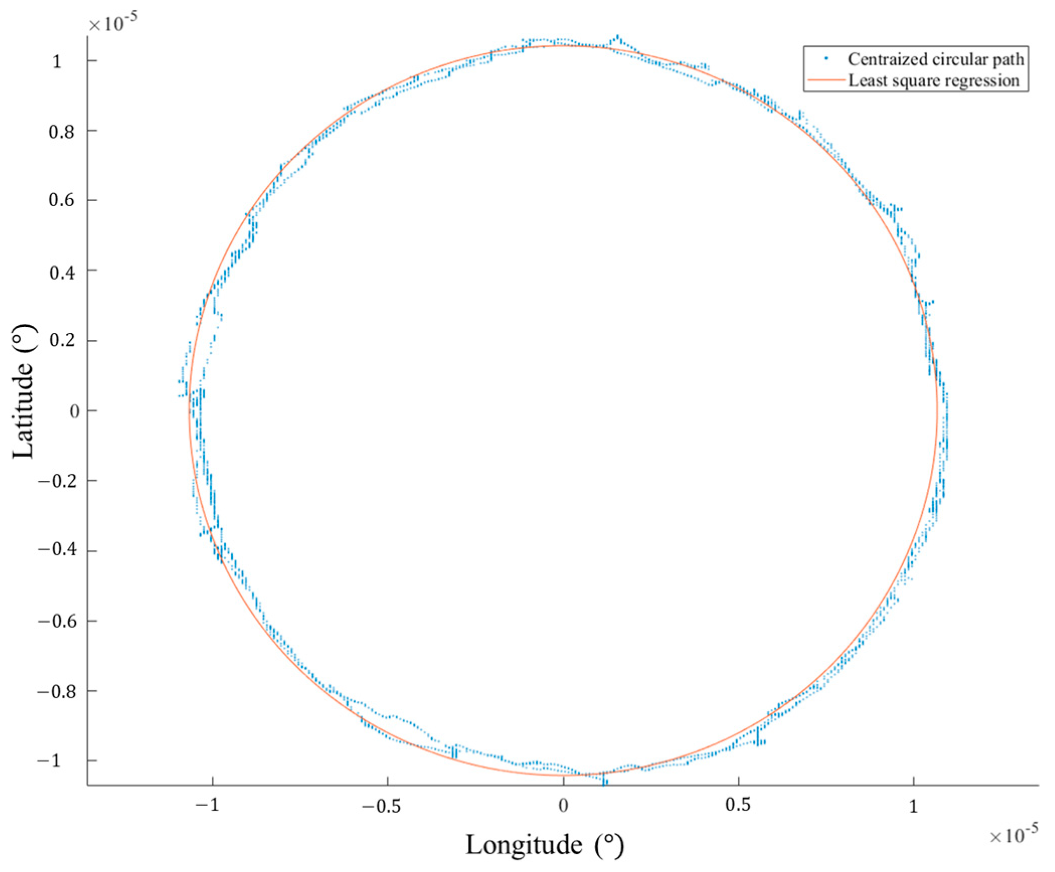
To ensure accurate localization in local Cartesian coordinates, a calibration procedure was performed to convert GNSS latitude–longitude data into a planar coordinate frame suitable for path planning. The micro EV was driven along a circular path, and the recorded GNSS points were fitted using ellipse least squares regression to determine the geographic conversion factors. This calibration enabled precise local mapping with minimal distortion.

Accurate geographic conversion is critical for trajectory prediction and waypoint tracking. If the GNSS data were directly used without calibration, small distortions in the coordinate transformation could lead to cumulative errors in vehicle localization and, consequently, in path-following accuracy. By establishing an accurate local frame, the predicted trajectories align consistently with the physical environment, improving both linear and angular deviation metrics during planning. This ensures that the planned candidate trajectories remain valid and that obstacle avoidance decisions are based on precise positional data. An example of the recorded GNSS trajectory and the fitted ellipse used for calibration is shown in Figure 6.

4. Experimental Setup

This section outlines the experimental setup used to evaluate the proposed autonomous navigation system. All tests were conducted on a closed-course environment to assess the vehicle’s path-following accuracy and obstacle avoidance capability under controlled conditions. The following subsections describe the test platform and environment, followed by the design of the path following and obstacle avoidance experiments.

4.1. Vehicle Platform and Test Environment

The test vehicle is a compact electric car retrofitted for autonomous control. It features an electronic steering actuator and dedicated throttle/brake systems, managed by an onboard high-level controller. Localization relies on a high-precision GNSS receiver with RTK correction, using a dual-antenna setup as shown in Figure 7a; the primary antenna is mounted near the rear axle, and a secondary antenna is positioned 1 m ahead along the centerline. A two-dimensional LIDAR scanner at the vehicle’s front provides complementary obstacle detection. All sensor data and control functions are handled by the onboard computer running custom navigation software.

All experiments were conducted on a closed-loop test track at Chulalongkorn University, shown in Figure 7b. The circular track allows the vehicle to start and end at the same point. The route was defined by manually driving the vehicle once to record a sequence of GNSS waypoints. Testing took place at night to minimize interference from traffic and pedestrians. Parts of the track are bordered by trees and buildings, creating areas of degraded GNSS quality, while most of the route remains open to the sky. Overall, the environment represents a typical low-speed campus road with a mix of open and partially obstructed conditions.

Figure 7. Experiment Setup: (a) test vehicle with the 2D laser scanner and the GNSS receiver installed, (b) test track located in Chulalongkorn University.

Figure 7. Experiment Setup: (a) test vehicle with the 2D laser scanner and the GNSS receiver installed, (b) test track located in Chulalongkorn University.

4.2. Path-Following Experiment

In the first phase of testing, the vehicle’s autonomous path-following ability was evaluated without obstacles. This phase established baseline tracking performance and allowed parameter tuning for later obstacle avoidance. Before field testing, the navigation algorithm, including the scored predicted trajectory planner, was validated in a custom simulator. The simulator assumed perfect trajectory tracking and was used to calibrate the control loop timing (~0.2 s) and initial scoring weights. These parameters served as the basis for real-world trials.

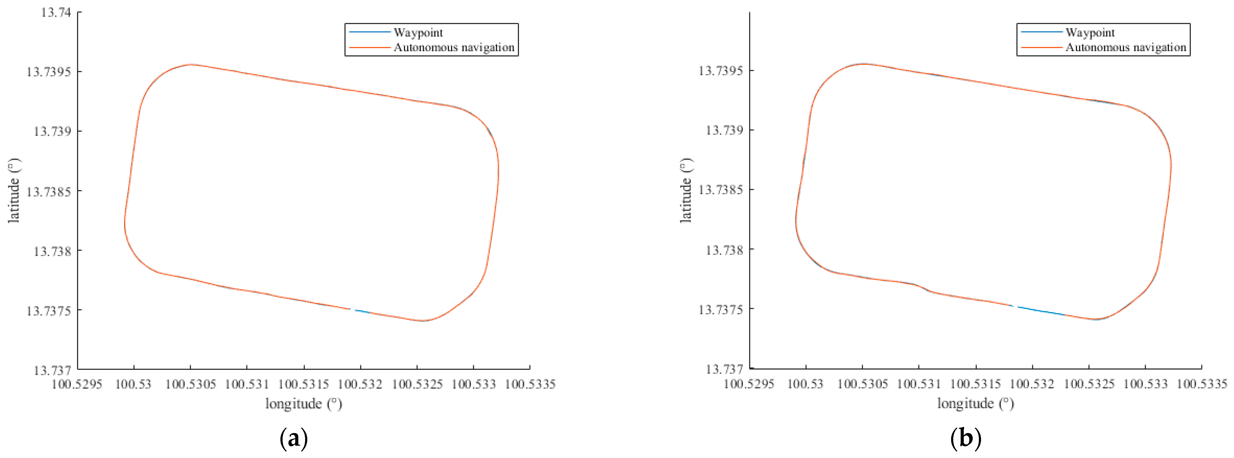
For field tests, the vehicle was placed at an arbitrary point on the closed-loop track and switched to the autonomous mode to follow prerecorded waypoints. The following two fixed speeds were tested: 10 km/h (nominal) and 15 km/h (system limit). The onboard controller managed speed and steering without manual intervention; a safety driver was present but never needed to intervene. During each trial, the GNSS position and heading were logged continuously for postprocessing. Tracking performance was analyzed by comparing the actual trajectory with the target waypoints, evaluating lateral deviations and heading errors. Figure 8a shows the recorded path at 10 km/h, closely matching the reference route, with similar results at 15 km/h as illustrated in Figure 8b.

4.3. Obstacle Avoidance Experiment

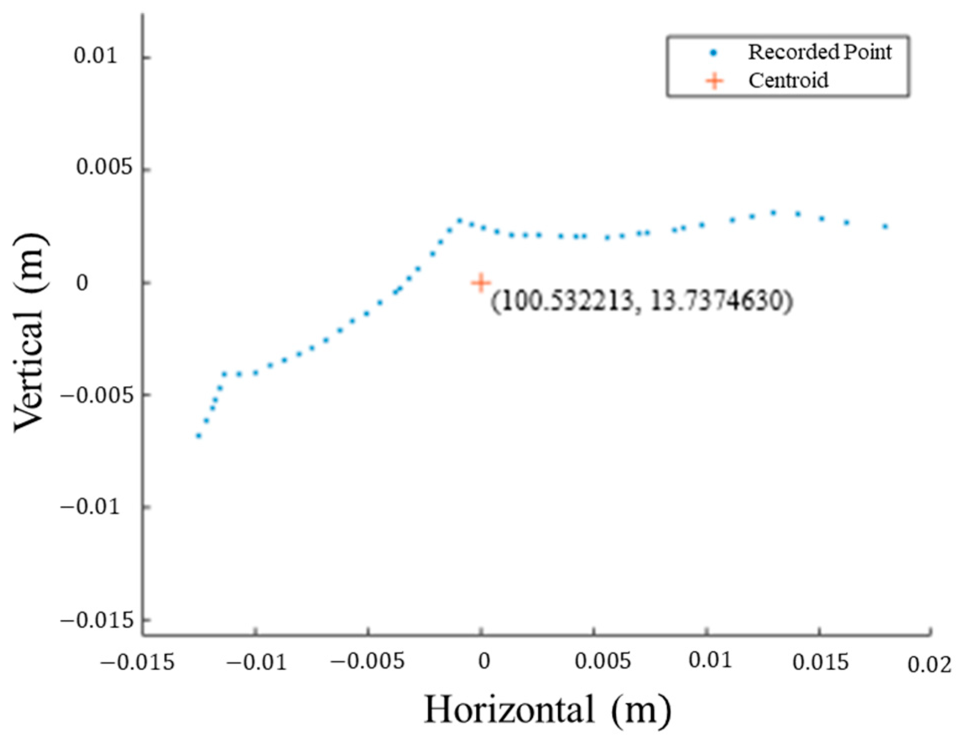
The second phase of experimentation evaluated the system’s obstacle avoidance capability. Trajectory-tracking parameters, including scoring weights, were set based on tuned values from the path-following tests. A single stationary obstacle was introduced onto the course to block the vehicle’s path and trigger an avoidance maneuver. Specifically, a traffic cone (or similar object) of approximately 0.4 m diameter was placed in the center of the lane along the waypoint route. The obstacle’s position was measured using the GNSS receiver to ensure precise placement relative to the predefined path. Multiple GNSS readings showed a variation of only about 4 cm horizontally and 2 cm vertically, indicating consistent positioning. In the vehicle’s internal map, the obstacle was modeled as a circular object of 0.4 m diameter, matching its physical size, for the path planner to avoid. The recorded GNSS position of the obstacle is shown in Figure 9.

In each obstacle avoidance trial, the autonomous vehicle followed the same looped route at 15 km/h. As it approached the obstacle, the onboard LIDAR detected the object, prompting the high-level controller’s scored predicted trajectory algorithm to dynamically adjust the course. The vehicle deviated from the original waypoints to steer around the obstacle and automatically merged back onto the predefined path afterward. This process tested the system’s ability to autonomously swerve and rejoin the route in real time. The obstacle avoidance scenario was executed in at least two runs to verify consistency and repeatability. In all trials, the vehicle successfully performed the avoidance maneuver without human intervention, demonstrating the effectiveness of the integrated GNSS-based path-following and LIDAR-based obstacle avoidance system.

This test environment was selected to emulate typical use cases of micro electric vehicles in semi-structured areas, where predefined routes and moderate obstacle density are common. The controlled layout ensures repeatability and consistency for evaluating localization accuracy and obstacle avoidance under realistic low-speed conditions.

5. Results

The autonomous navigation system was evaluated on a closed-loop test track in a campus environment. Experiments were conducted in the following two phases: first, to assess path-following accuracy at constant speeds (10 km/h and 15 km/h) and, second, to evaluate obstacle avoidance performance. Key quantitative results are presented below, with representative outcomes illustrated in Figure 10 and Figure 11 for path-following deviation analysis and Figure 12, Figure 13, Figure 14 and Figure 15 for obstacle avoidance behavior.

5.1. Path-Following Accuracy

In the path-following trials (with no obstacles), the vehicle consistently tracked the predefined waypoints with high accuracy. At 10 km/h, the lateral (linear) deviation from the target path had an average of approximately 0.13 m, while at 15 km/h, the average deviation was about 0.20 m. The distribution of lateral errors is depicted in Figure 10a and Figure 10b as histograms for 10 km/h and 15 km/h runs, respectively. These deviations are very small relative to the typical lane width (3.6 m), amounting to only about 3.6% of a lane’s width at 10 km/h (and ~5.6% at 15 km/h). The vehicle’s actual trajectory closely followed every recorded waypoint, as also evidenced by Figure 8a,b) (showing the GPS track overlaying the desired route).

Figure 10. The distribution of lateral errors: (a) speed at 10 km per hour, (b) speed at 15 km per hour.

Figure 10. The distribution of lateral errors: (a) speed at 10 km per hour, (b) speed at 15 km per hour.

Heading alignment was also maintained within acceptable limits. Figure 11 shows the distribution of heading (angular) deviation between the vehicle and the path. At 10 km/h, 95% of the heading error samples fell within ±2.65° to 1.85°, and for 15 km/h, within ±4.02° to 4.04°, indicating only a slight increase in heading error at the higher speed. In practice, the vehicle’s heading oscillated mildly around the path’s heading; this minor oscillation could cause a slight jerkiness in ride feel, but the magnitude of heading error (~3–4°) is negligible for navigation purposes and did not compromise lane-keeping accuracy. Overall, the path-following controller kept the vehicle well-aligned on the route, demonstrating the precise tracking of the waypoints.

Figure 11. Autonomous path following heading angle: (a) heading angle at 10 km per hour, (b) the distribution of heading errors at 10 km per hour, (c) heading angle at 15 km per hour, (d) the distribution of heading errors at 15 km per hour.

Figure 11. Autonomous path following heading angle: (a) heading angle at 10 km per hour, (b) the distribution of heading errors at 10 km per hour, (c) heading angle at 15 km per hour, (d) the distribution of heading errors at 15 km per hour.

As expected, increasing the speed from 10 km/h to 15 km/h had a small effect on the tracking performance. The standard deviation of the lateral deviation grew from about 0.07 m at 10 km/h to 0.12 m at 15 km/h, indicating slightly more variability at the higher speed. Similarly, the typical heading error range widened by a couple of degrees at 15 km/h. These results suggest that while the system remains accurate at 15 km/h, the vehicle’s dynamics (which begin to diverge from the pure kinematic model at higher speeds) introduce a bit more error. The kinematics-based trajectory model was sufficient for low-speed operation, but the degradation in precision at 15 km/h hints that a more complex vehicle model might be required to maintain the same level of accuracy at even higher speeds. Importantly, even in portions of the test loop where GNSS signals were partially obstructed by trees or adjacent buildings, the RTK-enabled localization maintained its accuracy; the vehicle still held roughly 10 cm average lateral error in those segments. This consistency under mild signal degradation highlights the robustness of the GNSS-based path following in the tested semi-structured environment.

5.2. Obstacle Avoidance Performance

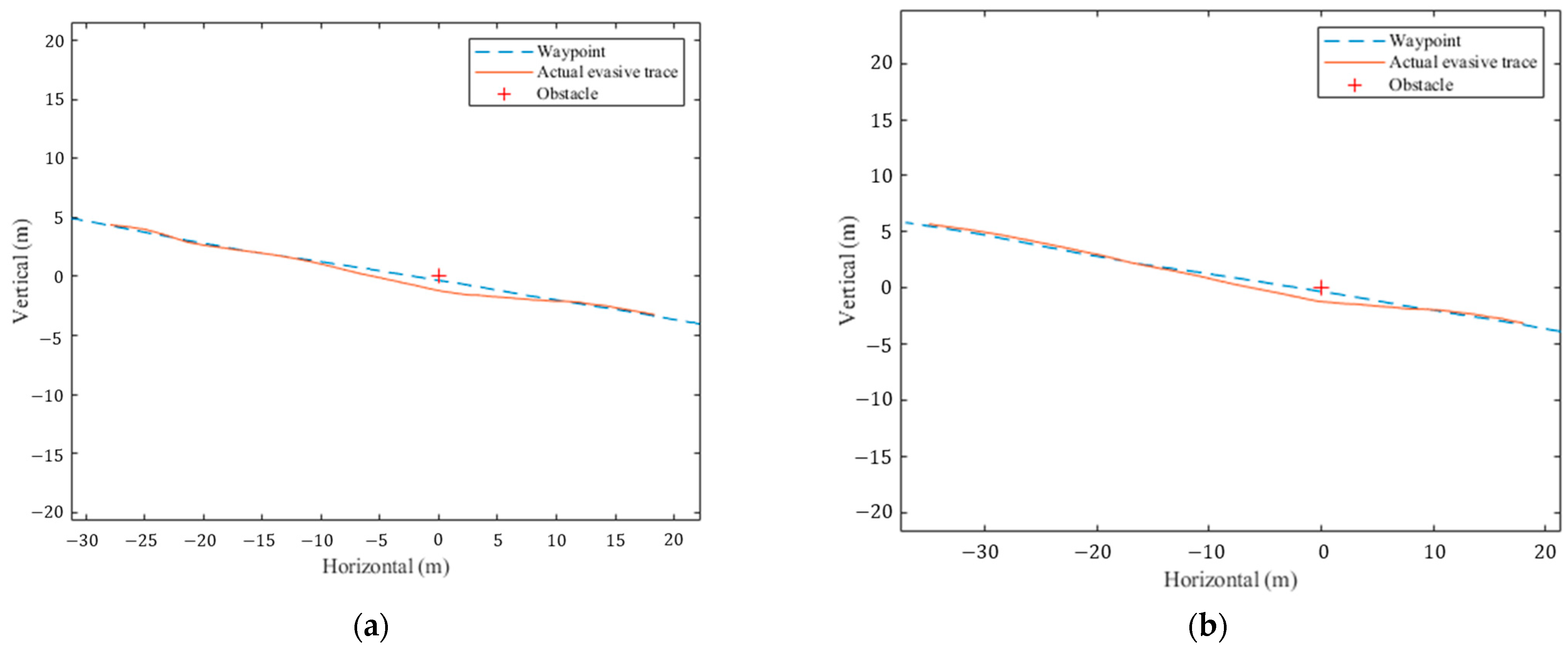
The obstacle avoidance functionality was validated by placing a static obstacle directly on the path and observing the vehicle’s response. Two trial runs were conducted (at 15 km/h) where the vehicle started following the waypoints normally until an obstacle was detected ahead. Figure 12 illustrates the vehicle’s trajectory during these trials. Initially, the autonomous car tracks along the right side of the path (moving from right to left in the figure). Upon detecting the obstacle in its forward path, the vehicle deviates from the waypoint trajectory, steering to the left to avoid a collision. After successfully passing the obstacle, the vehicle then steers back to the right and converges back onto the predefined path, resuming nominal tracking in the latter part of the run. This behavior is exactly as designed; the planner temporarily “ignores” the exact predefined path when a collision is imminent, then returns to the path once the obstacle no longer obstructs it.

Figure 12. Autonomous path following with obstacle avoidance result: (a) 1st experiment, (b) 2nd experiment.

Figure 12. Autonomous path following with obstacle avoidance result: (a) 1st experiment, (b) 2nd experiment.

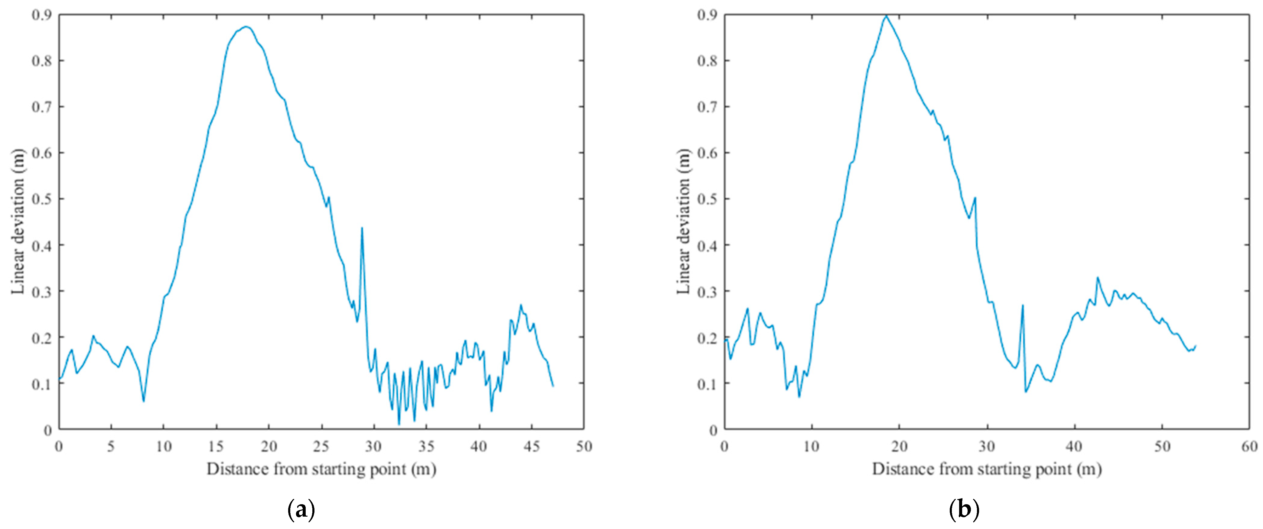
Quantitatively, the system’s performance during obstacle avoidance met the safety and path-following objectives. Figure 13 shows the lateral deviation from the path as a function of distance along the track for the two runs. At the beginning of each run, the lateral deviation stayed around 0.15–0.20 m (similar to the baseline path-following accuracy). However, at roughly 10 m before reaching the obstacle’s position along the route, the lateral error began to increase markedly. This corresponds to the point where the obstacle came within the vehicle’s predicted trajectory horizon (10 m), and the avoidance algorithm was triggered. The path-following controller yielded to the obstacle avoidance behavior at this point, causing the vehicle to depart from the waypoint—hence the spike in deviation. The peak deviation occurred as the vehicle passed the obstacle on a safe detour. After the obstacle, around 35 m beyond the point of deviation, the lateral deviation rapidly decreased as the vehicle merged back onto the original route. By the end of each trial, the steady-state deviation returned to near zero, indicating that the vehicle successfully re-aligned with the planned path after the evasive maneuver.

Figure 13. The lateral deviation from the path as a function of distance along the track: (a) 1st experiment, (b) 2nd experiment.

Figure 13. The lateral deviation from the path as a function of distance along the track: (a) 1st experiment, (b) 2nd experiment.

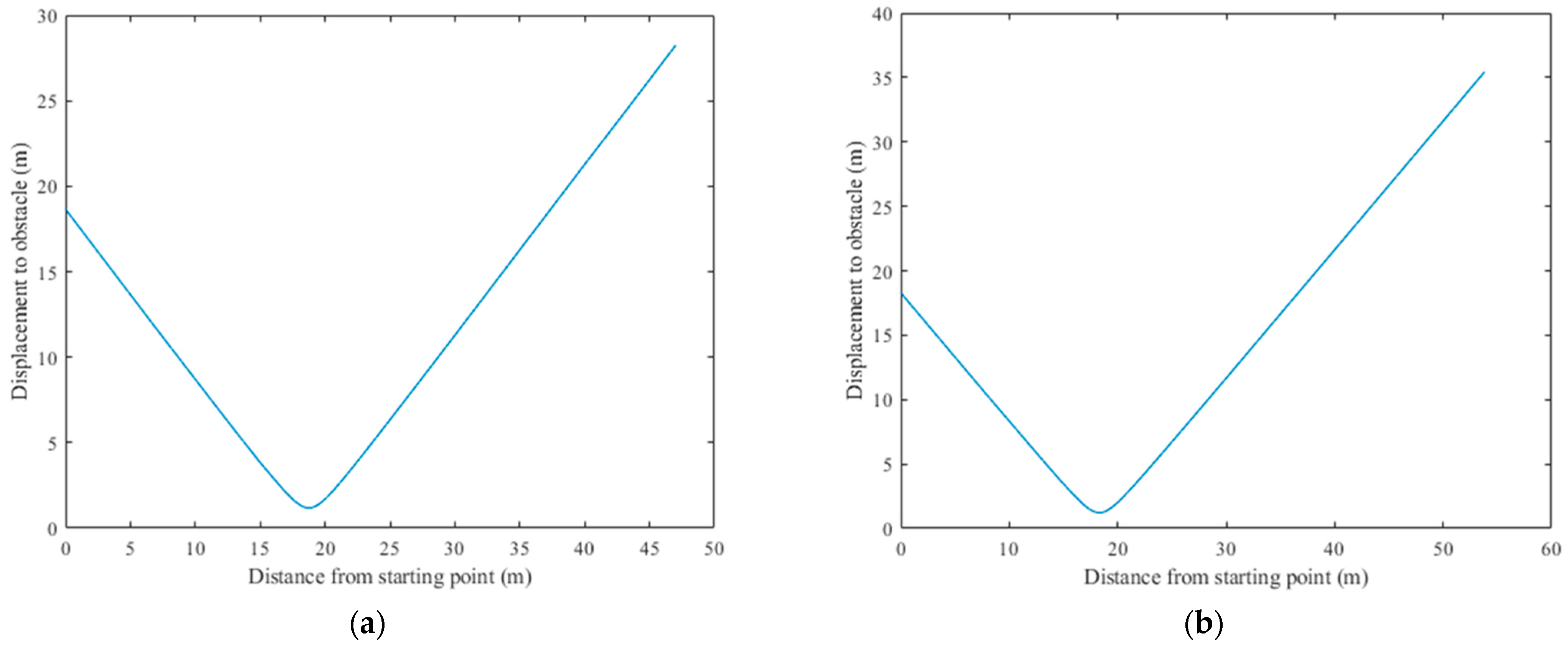
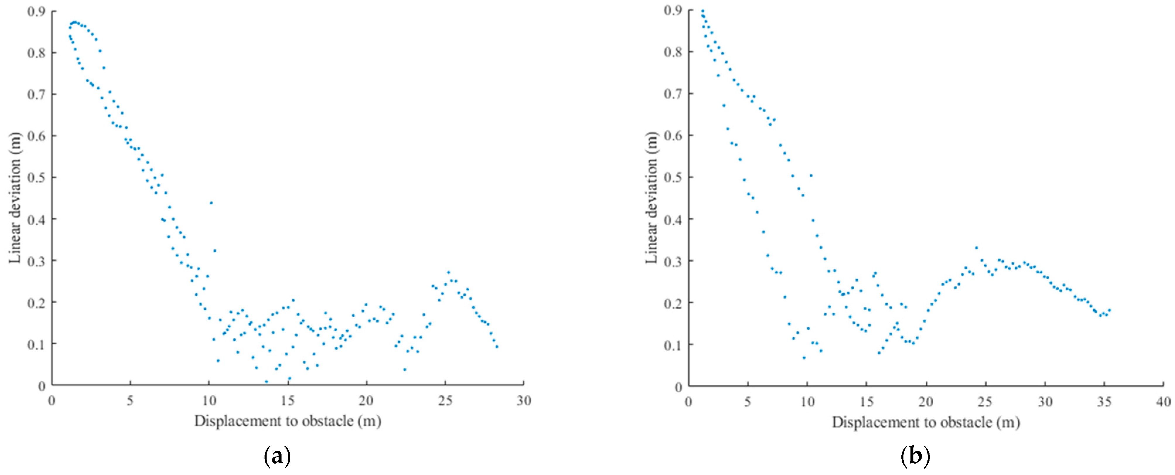
The distance to the obstacle throughout the encounter is plotted in Figure 14 for the two experiments. The minimum distance between the vehicle and the obstacle was maintained at approximately 1.2 m, never dropping below about 1.19 m in either trial. This clearance matches the configured safety buffer in the system’s parameters (1.2 m) and demonstrates that the vehicle passed the obstacle with the intended margin of safety. The relationship between path deviation and obstacle proximity is further illustrated in Figure 15, which plots lateral deviation versus distance to the obstacle. These figures confirm that as soon as the obstacle came within roughly 10 m of the vehicle, the lateral deviation began to increase (i.e., the vehicle started to veer off the original path), and conversely, once the obstacle was beyond the vehicle (distance increasing again), the deviation came down. In effect, the obstacle avoidance module took over control authority at about a 10 m threshold of obstacle distance, which corresponds to the chosen lookahead (trajectory length) of the planner. The vehicle then kept a wide berth around the object and smoothly returned to the path after clearing it. Overall, the obstacle avoidance experiments demonstrated that the scored predicted trajectory approach successfully balances path tracking with reactive evasion; the car avoided the obstacle in both trials without any collision or stall, and it rejoined the original path with only a transient deviation. The results validate that the system can handle sudden obstacles on the route, maintaining safety (no contact, minimum ~1.2 m clearance), while eventually achieving the navigation goal.

Figure 14. Displacement to obstacle at any instance: (a) 1st experiment, (b) 2nd experiment.

Figure 14. Displacement to obstacle at any instance: (a) 1st experiment, (b) 2nd experiment.

Figure 15. Path deviation and obstacle proximity: (a) 1st experiment, (b) 2nd experiment.

Figure 15. Path deviation and obstacle proximity: (a) 1st experiment, (b) 2nd experiment.

To evaluate the system’s robustness under different operating conditions, multiple test scenarios were conducted, including varying vehicle speeds (10 km/h and 15 km/h) and obstacle configurations. The system’s performance was assessed based on lateral deviation, heading error, and minimum obstacle clearance. The results demonstrate consistent path-following accuracy and safe obstacle avoidance behavior across all configurations. A summary of these experimental outcomes is provided in

Table 1. Summary of system performance under different test configurations.

Configuration	Lateral Deviation (m)	Heading Error (deg.)	Obstacle Clearance (m)
10 km/h, no obstacle	0.13 (mean), 0.07 (std)	~1.13 (mean), within ±2.65	-
15 km/h, no obstacle	0.20 (mean), 0.12 (std)	~2.02 (mean), within ±4.04	-
15 km/h, with obstacle (trial 1/2)	0.15–0.20 (peak)	~3.5–4.0	1.2 m

.

5.3. Robustness Under GNSS Degradation

An important aspect of performance is how the system handles GNSS signal degradation, as localization primarily relies on GNSS with RTK corrections. During field tests, sections of the track bordered by trees and buildings impaired satellite reception. Despite this, the vehicle maintained precise navigation, with average waypoint tracking errors around 10 cm even under canopy cover. The RTK-enabled GNSS provided robust position fixes, and short-term occlusions or multipath effects did not significantly impact accuracy. This demonstrates resilience to moderate GNSS obstruction in semi-structured environments.

However, the system’s robustness has limits. No prolonged GNSS outages occurred during testing—the vehicle never lost the RTK fix. The current architecture lacks odometry or inertial navigation to bridge coverage gaps. A severe or extended GNSS dropout, such as in tunnels or urban canyons, would challenge the system. Supplementary simulations showed that even a one-minute GNSS loss could cause positional uncertainty to grow unbounded. In practice, complete signal loss is unlikely in the intended environments (e.g., campus roads), and minor degradations had minimal impact. Nonetheless, achieving full reliability under GNSS-denied conditions would require additional sensors or techniques, which is beyond the scope of this design. In summary, the system proved robust within GNSS-friendly, semi-structured settings but remains dependent on continuous GNSS availability for long-term navigation.

6. Discussion

The experimental results demonstrate that the proposed GNSS-based autonomous navigation system achieves a practical balance of accuracy, safety, and simplicity. Using high-precision RTK GNSS, the system achieved ~0.1–0.2 m path-following error without complex map building or camera-based perception, reaching accuracy comparable to SLAM systems with a simpler method. Safety is ensured through a 2D LiDAR for obstacle detection and a conservative avoidance strategy, maintaining about 1.2 m clearance from obstacles. The system’s simplicity—minimal sensors and lightweight predictive trajectory scoring—reduces cost and complexity, making it easier to implement and maintain than many advanced platforms. Thus, the system provides adequate accuracy and safety for low-speed autonomous driving in structured environments at a relatively low cost.

This GNSS-centric navigation approach is well-suited to semi-structured environments like university campuses, industrial parks, or factory roads, where low speeds, predefined routes, and moderate obstacle density are common. Open skies enable RTK GNSS use, and the predictable environment makes a 2D LiDAR sufficient for obstacle detection. The campus test track exemplified this, confirming the system’s suitability for controlled domains where deploying high-end sensors may not be practical. It offers a cost-effective solution for applications like campus shuttles, gated communities, or factory logistics, where GNSS corrections are feasible, and predefined mapping suffices.

Despite its strengths, the system has limitations. It relies entirely on GNSS for localization; while RTK GNSS is robust outdoors, it degrades in urban canyons, in dense foliage, or indoors. Without odometry or inertial backup, prolonged GNSS outages would compromise navigation. The 2D LiDAR restricts perception to a horizontal plane, missing overhead or terrain variations, and its limited range may not suffice for faster vehicles or complex environments. The control and planning algorithms, based on a kinematic bicycle model, are tuned for low speeds (~15 km/h), with slight tracking degradation observed at higher speeds. Additionally, obstacle avoidance was tested only against static obstacles; more complex scenarios with dynamic obstacles would require algorithmic improvements.

When compared to ROS-based SLAM systems, which build maps and localize without GPS, our approach avoids the need for expensive 3D LiDARs or high computational resources, though it cannot operate in GNSS-denied areas. Visual–inertial odometry (VIO) systems provide greater autonomy without external signals but suffer from drift over time. Our GNSS-based system benefits from absolute localization without drift, ideal for repetitive routes, though pure VIO would outperform it indoors or under dense canopies. Hybrid systems combining GNSS with IMU or odometry could enhance robustness, and such integration is a potential future improvement.

Compared to full-stack autonomous systems, which use multi-modal sensors and heavy computing for high-speed, complex driving, our minimalist design achieves reliable autonomy with only RTK GNSS, a low-cost LIDAR, and lightweight algorithms. This makes it attractive for applications where cost, power, and simplicity are priorities, such as factories or private campuses.

The proposed navigation system was implemented on an Intel Core i7-based embedded PC, selected for its balance between performance and power efficiency. The trajectory planning algorithm evaluates 27 candidate paths per cycle using a memory resident profile table and algebraic scoring, enabling efficient real-time execution. The full sense–plan–act cycle runs at 10 Hz, with average planning latency around 10 ms, allowing timely response to dynamic obstacles. Despite involving multiple modules—GNSS-RTK processing, LiDAR-based obstacle detection, and predictive trajectory scoring—the system maintains CPU usage at a manageable level without relying on GPU acceleration. These results demonstrate the suitability of the proposed architecture for real-time deployment in micro EV platforms with limited computational resources.

Although no direct experimental comparisons were performed against specific baseline planners, such as DWA, SLAM, or DRL-based methods, the achieved performance under different configurations was analyzed. The system was evaluated at two speeds (10 km/h and 15 km/h), with and without static obstacles. Results showed average lateral deviations ranging from 0.07 m to 0.20 m, heading errors from ~1.1° to 4°, and consistent obstacle clearance of 1.2 m. Table 1 summarizes the performance under each condition. The achieved performance of our system demonstrates that low-complexity, GNSS-based navigation can be viable for micro EVs operating in semi-structured environments. While many recent studies have focused on more advanced techniques—such as deep learning-based obstacle avoidance, multi-sensor fusion with IMU and LiDAR, or cloud-coordinated frameworks for connected vehicles—these often come at the cost of increased hardware and computational demands. For example, approaches involving RTK-GNSS combined with inertial or visual sensors [3,4,14,21,22] provide high precision but require tight sensor integration and robust processing capabilities. In contrast, the proposed system utilizes only RTK-GNSS and a 2D LiDAR sensor, achieving lateral accuracy within 0.2 m and maintaining a 1.2 m clearance from obstacles. This validates the potential of minimal-sensor configurations for reliable low-speed autonomy in structured outdoor scenarios. Future work will explore direct benchmarking with these more complex frameworks to further quantify trade-offs.

From a safety perspective, deploying autonomous systems in public environments requires reliable failsafe mechanisms, consistent behavior under uncertain conditions, and real-time responsiveness to pedestrians and other road users. Although our system was validated in a closed campus setting, further testing under varied environmental conditions, including more unpredictable and dynamic scenarios, is necessary to ensure safety compliance. Incorporating redundant sensing or emergency braking logic may also be required before real-world deployment.

The experimental setup was intentionally designed to match the system’s target application domain—low-speed autonomous navigation in semi-structured environments such as university campuses, factory roads, or gated communities. The use of a closed-loop track with predefined waypoints and static obstacles enabled controlled evaluation of path following and obstacle avoidance performance. Although this setting may appear limited, it reflects common real-world deployment conditions for micro EVs, where routes are known, and dynamic hazards are relatively infrequent. We acknowledge that the current experimental content is narrow in scope; future work will include testing under more diverse conditions, such as dynamic obstacles, variable terrain, GNSS-degraded areas, and higher speeds, to fully evaluate system robustness.

In summary, the proposed system achieves a practical trade-off, combining precise satellite-based localization with basic yet effective obstacle avoidance. Its experimental validation confirms high path-following accuracy and safe navigation with minimal infrastructure. Although limited to GNSS-friendly, structured environments, it offers a compelling balance of performance, simplicity, and cost-effectiveness for targeted autonomous applications.

7. Conclusions

This research successfully achieved the three major objectives of developing an autonomous navigation system for a micro electric vehicle. First, a low-level control system for steering, acceleration, and braking was designed and integrated into the Toyota COMS platform, enabling full autonomous control, while retaining manual over-ride capability. Second, a high-level navigation system based on GNSS-RTK localization and a scored predicted trajectory planning algorithm was developed, allowing accurate waypoint tracking with minimal computational requirements. Third, real-time obstacle avoidance was implemented and validated, ensuring safe navigation in the presence of unexpected hazards.

The system was experimentally validated under multiple real-world configurations, including vehicle speeds of 10 km/h and 15 km/h and scenarios with static obstacles. Results demonstrated lateral tracking errors between 0.07 m and 0.20 m and heading deviations ranging from ~1.1° to 4°, with a consistent minimum obstacle clearance of 1.2 m. The system maintained robust navigation even in areas with partial GNSS signal degradation. These results confirm that the proposed approach achieves reliable, accurate, and safe performance using only RTK-GNSS and a 2D LiDAR sensor—without reliance on complex sensor fusion or high-performance computing. Compared to SLAM- or IMU-integrated systems, this setup offers a simpler yet competitive alternative for structured and semi-structured environments.

However, the system’s reliance on GNSS and 2D LiDAR imposes limitations in GNSS-denied environments or highly dynamic scenes. For future improvements, incorporating low-cost inertial sensors or wheel odometry could enhance robustness during GNSS outages. Replacing the relatively expensive 2D LiDAR with more cost-effective alternatives and integrating a more advanced vehicle dynamics model may further extend the system’s applicability to higher-speed operations. Future work will also include testing the system with dynamic obstacles to assess real-time responsiveness under more complex conditions.

In terms of regulatory considerations, the public deployment of autonomous micro EVs may require compliance with local vehicle automation standards, safety certification, and operational restrictions (e.g., speed limits, geofencing). While the current system shows promise in controlled domains, adapting it for public roads will require additional validation and regulatory alignment.

Overall, the proposed solution presents a practical, low-cost framework for low-speed autonomous navigation in semi-structured environments, such as campuses, gated communities, and industrial areas.