Abstract
This study proposes a hybrid framework for rolling bearing fault diagnosis by integrating a Variational Mode Decomposition–Discrete Wavelet Transform (VMD-DWT) with a Hybrid Attention-Based Depthwise Separable CNN-BiLSTM (HADS-CNN-BiLSTM) to address noise interference and low diagnostic accuracy under complex conditions. The vibration signals are first reconstructed using a genetic algorithm (GA)-optimized VMD and particle swarm optimization (PSO)-optimized DWT for noise suppression. Subsequently, the denoised signals undergo multimodal feature fusion through depthwise separable convolution, triple attention mechanisms, and BiLSTM temporal modeling. The hybrid model incorporates dynamic learning rate scheduling and a two-stage progressive training strategy to accelerate convergence. The experimental results on the Case Western Reserve University (CWRU) dataset demonstrate 99.58% fault diagnosis accuracy in precision, recall, and the F1 Score, while achieving 100% accuracy on the Xi’an Jiaotong University (XJTU-SY) dataset, confirming superior generalization and robustness under varying signal-to-noise ratios. The framework provides an effective solution for enhancing rolling bearing fault diagnosis technologies.
1. Introduction
Bearings serve as critical components in rotating machinery, widely implemented in mechanical transmission systems of large-scale equipment such as electric motors, gearboxes, and cranes [1]. The increasing complexity of mechanical structures and progressively extreme operating conditions have subjected rolling bearings to more severe operational loads, thereby heightening their susceptibility to failure [2]. The operational state of bearings directly governs equipment functionality, reliability, and safety, with potential failures potentially triggering system breakdowns and substantial economic losses [3]. Consequently, continuous reliability monitoring of rolling bearings has become imperative [4,5]. Vibration signals constitute essential information sources for condition monitoring, and are recognized as the most accurate indicators of bearing performance and the prevalent choice for fault diagnostics [6]. Researchers often employ Fourier transform, envelope analysis, spectral kurtosis, Wavelet Transform, and Empirical Mode Decomposition to process bearing vibration signals [7]. Bearing fault detection methodologies primarily consist of two sequential stages: feature extraction and fault identification [8].
Fault characteristics can be extracted from temporal and frequency domains. However, the non-stationary and nonlinear nature of bearing vibration signals under actual operating conditions complicates accurate feature extraction, adversely affecting diagnostic accuracy [9]. Time-frequency analysis serves as a prevalent signal processing approach for characterizing signal variations across both domains. Commonly employed techniques include Short-Time Fourier Transform (STFT), Empirical Mode Decomposition (EMD), Variational Mode Decomposition (VMD), and Wavelet Transform (WT). Classical bearing fault diagnosis methods include Hilbert transform-based (envelope analysis) and the SPM (Shock Pulse Method). Wang et al. [10] directly used the entire Hilbert envelope spectrum of the resampled signal as a feature vector to characterize bearing fault types and established a DBN classifier model to identify bearing faults. However, background noise in the original vibration signal may persist in the envelope spectrum after Hilbert transform, particularly high-frequency noise, which could be misinterpreted as fault features. Zhang et al. [11] combined the Shock Pulse Method with frequency analysis for early bearing fault detection. However, the Shock Pulse Method is highly dependent on rotational speed. At low speeds, the impact signals may be too weak for reliable detection, while at high speeds, increased noise may mask genuine fault signals.
Geraei et al. [12] developed a bearing fault detection methodology integrating Adaptive Local Binary Patterns (ALBPs) with STFT. Unlike conventional Fourier analysis providing global frequency information, STFT dissects signals into short-duration segments through window functions (e.g., Hann, rectangular) that decay to zero beyond specified intervals, followed by Fourier transformation of each segment. This localized analysis enables spatiotemporal fault localization within mechanical systems.
Wang et al. [13] also utilized STFT to convert one-dimensional time-domain vibration signals of bearings into two-dimensional time-frequency images, which were then input into a generative adversarial network for bearing fault diagnosis. Nevertheless, STFT’s efficacy critically depends on predefined window parameters (shape and length), which remain fixed regardless of signal characteristics. As STFT essentially constitutes superposed windowed Fourier transforms, noise contamination inevitably corrupts time-frequency distributions—particularly detrimental under low signal-to-noise ratio conditions. Qi et al. [14] utilized EMD to decompose bearing vibration signals, subsequently feeding the IMFs into a hierarchical 1D Convolutional Neural Network (1D-CNN) for fault classification. However, high-frequency impact components in bearing fault signals may spectrally overlap with low-frequency background noise within the same IMF, resulting in frequency masking that compromises diagnostic precision. Taibi et al. [15] implemented VMD to disassemble raw bearing vibration signals into multiple IMFs, followed by Discrete Wavelet Transform (DWT) for noise-IMF filtration and feature extraction in motor bearing diagnostics. Notably, VMD requires predefined parameters (decomposition mode count k and penalty factor α), whose selection lacks theoretical guidance and relies on empirical or trial-and-error approaches. Li et al. [16] employed genetic algorithms to optimize the decomposition level and penalty factor in VMD for rolling bearing fault diagnosis across the full life cycle. Compared to other optimization algorithms such as the whale optimization algorithm (WOA), genetic algorithms leverage population diversity (through crossover and mutation operations) and global parallel search mechanisms to explore multiple potential optimal solutions in multidimensional parameter spaces, effectively avoiding local optima and making them an excellent choice for VMD parameter optimization. Liu et al. [17] proposed an interpretable domain-adaptive Transformer (IDAT) method for cross-condition and cross-machine bearing fault diagnosis. The core of this approach involves using a multi-layer domain-adaptive Transformer to extract useful features, with interpretation provided through multi-head attention maps. However, processing multiple feature subspaces in parallel via multi-head attention leads to exponentially increasing computational demands for bearing vibration signals, particularly with long time series or high-resolution time-frequency images, significantly increasing the computational burden. Yu et al. [18] developed a post-processing time-frequency analysis (TFA) method termed a Wavelet-Based Time Synchro Extracting Transform (WTSET) to precisely capture fault characteristic frequencies in flexible thin-walled bearings. This technique enhances time-frequency representation (TFR) energy concentration while maintaining signal invertibility. Lu et al. [19] employed wavelet thresholding (WT) denoising to process the acquired bearing vibration signals, effectively reducing noise interference. The diagnostic efficacy of wavelet-based methods inherently depends on wavelet basis function selection (ψ) and the decomposition level (L). Different combinations of ψ and L exhibit significant variability in feature representation capabilities, yet their optimization lacks systematic theoretical frameworks and requires empirical determination.
Following feature extraction from vibration signals, the subsequent fault classification phase typically employs diagnostic models including Decision Trees, support vector machines (SVMs), k-nearest neighbors (K-NNs), Naive Bayes classifiers, convolutional neural networks (CNNs), and long short-term memory (LSTM) networks. Briglia et al. [20] implemented Decision Tree technology for motor bearing fault detection using power current signatures, where tree structures are inductively learned from observational data to enable straightforward fault categorization through path traversal. The Decision Tree algorithm recursively partitions the feature space, yet its performance diminishes significantly in high-dimensional spaces while tending to generate overcomplex structures prone to overfitting. Wang et al. [21] proposed a rolling bearing fault diagnosis technique based on recurrence quantification analysis (RQA) and a Bayesian-optimized support vector machine (RQA-Bayes-SVM). The Bayesian optimization algorithm was employed to search for the optimal penalty factor C and kernel function parameter g of the SVM, thereby establishing an optimal Bayes-SVM model. Maincer et al. [22] applied SVM and K-NN methodologies for robotic manipulator fault diagnosis, employing Gaussian kernel-based SVM optimized via particle swarm optimization (PSO) to maximize diagnostic accuracy. Sun et al. [23] developed a k-NN attention-enhanced Video Vision Transformer (k-ViViT) network for action recognition, substituting conventional self-attention with k-NN attention to mitigate noise interference from irrelevant tokens. SVM performance critically depends on kernel selection (linear, polynomial, radial basis function) and parameter tuning (regularization parameter C, kernel coefficient γ). Suboptimal parameter combinations degrade model efficacy, necessitating computationally intensive cross-validation and grid search procedures. In contrast, K-NN suffers from computational inefficiency in high-dimensional feature spaces and large datasets due to its exhaustive distance calculation requirements between query instances and all training samples. Peretz et al. [24] proposed an enhanced naïve Bayes classifier method for multidimensional and multivariate datasets, termed the Naïve Bayes Enrichment Method (NBEM). This method employs multiple naïve Bayes classifiers based on different distributions and their combinations to classify new observations. However, as a probabilistic model, naïve Bayes classifiers rely on the probability distribution of the training data; significant discrepancies between the distributions of training and testing data may limit the model’s generalization capability.
Ni et al. [25] constructed a dual-stream convolutional neural network (CNN) model for bearing fault diagnosis. The first stream processes 1D vibration signal spectra, while the second stream handles 2D time-frequency representations derived from the same signals. CNNs extract local features through convolutional layers, which may inadequately capture global features or complex spatiotemporal relationships in certain fault diagnosis scenarios. Chen et al. [26] designed a neural network model called multi-scale CNN-LSTM (convolutional neural network-long short-term memory) combined with a deep residual learning model for rolling bearing fault diagnosis. This architecture integrates multi-scale wide CNN-LSTM modules with deep residual modules. Han et al. [27] proposed a hybrid diagnostic method combining convolutional neural networks (CNNs), long short-term memory (LSTM) networks, and gated recurrent unit (GRU) models. In this approach, the output processing of the CNN embeds LSTM networks to analyze long-sequence variation characteristics of rolling bearing vibration signals, enabling long-term time series prediction by capturing long-range dependencies in the sequences. Xu et al. [28] developed a multi-level residual convolutional neural network with dynamic feature fusion (MRCNN-DFF) for mechanical fault diagnosis. The MRCNN-DFF incorporates depthwise separable (DS) convolution to reduce the number of trainable parameters, offering advantages in model optimization and improving optimization efficiency.
In the CNN-LSTM architecture, unidirectional LSTM may overlook reverse causal relationships, whereas BiLSTM can simultaneously capture both forward and backward temporal dependencies in fault signals. The dense convolutional layers in CNN typically involve a large number of parameters. This computational burden can be reduced by decomposing standard convolution into depthwise convolution and pointwise convolution. The static convolution operations in CNN-LSTM demonstrate limited effectiveness in suppressing noise interference. To address this limitation, a Hybrid Attention module integrating channel attention and spatial attention can be employed. This module dynamically enhances critical fault features through energy gating. Regarding hyperparameter tuning in CNN-LSTM, the manual adjustment of learning rates and other parameters often lacks precision. This challenge can be mitigated by implementing a random search for automated hyperparameter optimization and adopting dynamic learning rate scheduling. Building upon the CNN-BiLSTM fault classification framework, we propose an enhanced architecture: the Hybrid Attention-Based Depthwise Separable CNN-BiLSTM (HADS-CNN-BiLSTM) model.
Based on the comprehensive analysis above, this study proposes a bearing fault diagnosis method integrating algorithm-optimized VMD-DWT with the HADS-CNN-BiLSTM model to address the challenges of low diagnostic accuracy. To reduce strong noise interference and resolve parameter configuration difficulties in VMD and DWT decomposition, the genetic algorithm (GA) is utilized to optimize VMD parameters (decomposition modes k and penalty factor α) using permutation entropy (PE)–kurtosis (K) as the objective function. The correlation coefficients between each IMF and the original signal are calculated. IMFs with coefficients less than or equal to 0.1 are directly discarded. Those with coefficients between 0.1 and 0.8 undergo further wavelet transformation, while components with coefficients greater than 0.8 are retained. The PSO algorithm optimizes the DWT parameters (optimal wavelet basis and decomposition level) based on the minimum Root Mean Square Error (RMSE) criterion to perform secondary denoising on IMFs with coefficients in the 0.1 to 0.8 range. The denoised IMFs and retained components are then reconstructed. After feature extraction from the reconstructed signals, the features are input into the HADS-CNN-BiLSTM model for fault diagnosis. The experimental results demonstrate that this method effectively improves bearing fault diagnosis accuracy and exhibits promising application prospects. The main contributions of this study are as follows:
- (1)
- GA-optimized VMD parameters: addressing the difficulty in selecting decomposition modes k and penalty factor α, GA automates parameter optimization, eliminating reliance on empirical selection through extensive manual experimentation.
- (2)
- PSO-optimized DWT parameters: solving the challenge of wavelet basis and decomposition level selection in DWT denoising, PSO prevents incomplete noise reduction.
- (3)
- VMD-DWT signal reconstruction: the proposed reconstruction method significantly reduces strong noise interference on useful vibration signals, providing reliable data support for bearing fault diagnosis and condition monitoring.
- (4)
- The HADS-CNN-BiLSTM framework is constructed by integrating advanced techniques such as depthwise separable convolution, hybrid attention mechanisms, and BiLSTM. Specifically optimized for industrial fault diagnosis tasks, the proposed method is validated on two public datasets to demonstrate its effectiveness.
The remainder of this paper is organized as follows: Section 2 “ Signal processing methods”: introduces the noise reduction process of raw signals through GA-optimized VMD and PSO-optimized DWT, followed by signal reconstruction. Section 3 “The proposed model”: details the complete workflow of the improved VMD-DWT and HADS-CNN-BiLSTM fault diagnosis framework. Section 4 “Experimental validation”: validates the diagnostic accuracy of the method using the CWRU and XJTU-SY bearing datasets. Section 5 “Conclusions”: summarizes the key research findings.
2. Signal Processing Methods
2.1. Parameter-Optimized Variational Mode Decomposition Using Genetic Algorithm
Suppose we have an observed signal . The objective of VMD is to decompose it into k ode signals (k = 1, 2, ⋯, K), each with distinct center frequencies. These modes must satisfy the following two conditions: (a) The spectral distribution of each mode is concentrated within a specific frequency band. (b) The modes are mutually orthogonal, i.e., their spectra exhibit sufficient separation in the frequency domain. The VMD formulation aims to minimize the sum of estimated bandwidths for all modes while satisfying the constraint that the sum of all modes equals the original signal. The variational problem is expressed as follows:
where denotes the partial derivative with respect to time, is the Dirac delta function, ∗ represents the convolution operator, and is the imaginary unit.
To solve the aforementioned constrained optimization problem, we transform it into an unconstrained formulation by introducing a Lagrange multiplier and a quadratic penalty parameter α. The augmented Lagrangian function is derived as follows:
where ∗ denotes the convolution operation. The Alternating Direction Method of Multipliers (ADMMs) is employed to iteratively update the mode signals , center frequencies , and Lagrange multiplier . The mathematical formulation is expressed as follows:
the iterations are repeated until the objective function converges or the preset precision tolerance (tol) is reached, as follows:
As evident from the VMD decomposition process, the mode number k and penalty factor α are two critical parameters governing the quality of VMD results. An improperly chosen k may lead to over-decomposition or under-decomposition, while an inappropriate α could cause information loss or spectral redundancy. The optimization of VMD parameters presents distinct challenges; the mode number k requires integer values while the penalty factor α is continuous. Genetic algorithms (GAs) inherently support mixed encoding schemes, naturally accommodating both parameter types. In contrast, the whale optimization algorithm (WOA) and gray wolf optimizer (GWO) necessitate the artificial discretization of k, potentially introducing quantization errors. This fundamental difference gives GA a natural advantage for VMD parameter optimization. To address this issue, this paper proposes a GA-driven optimization strategy to determine the optimal (k,α) combination.
We establish a PE–kurtosis parameter optimization criterion. PE, a statistical measure for quantifying the complexity of time series signals, is calculated by determining the occurrence probability of each permutation pattern π. This is achieved by counting the frequency of each permutation pattern across all reconstructed vectors. The PE is defined as follows:
where the summation extends over all possible permutation patterns π.
Kurtosis (K) measures the peakedness of a signal waveform and is commonly used to detect anomalies or impulsive components in signals. For a dataset , the K is defined as follows:
where denotes the expected value operator, μ is the mean of dataset X, σ is the standard deviation of X, and σ is defined as follows:
Considering the respective advantages of both approaches, this paper proposes a permutation entropy–kurtosis parameter optimization criterion that synergistically combines .
The definition is calculated as follows:
where is the average permutation entropy of each IMF under the current (k, α) parameters, and is the average kurtosis of each IMF component under the current (k, α) parameters. This not only considers the correlation between components and the original signal but also effectively reflects the degree of periodic pulses and impact components in the signal, more comprehensively preserving fault information. Compared to single indicators that only focus on impact strength or correlation, it combines the advantages of both indicators. A larger kurtosis value indicates stronger impact characteristics of the signal; a smaller permutation entropy indicates better correlation and periodicity of the signal. Therefore, a smaller value represents richer fault features and better noise reduction effects. The permutation entropy–kurtosis parameter optimization criterion uses genetic algorithms to obtain the minimum value, at which point (k, α) becomes the optimal combination of parameters for the VMD decomposition of the current signal.
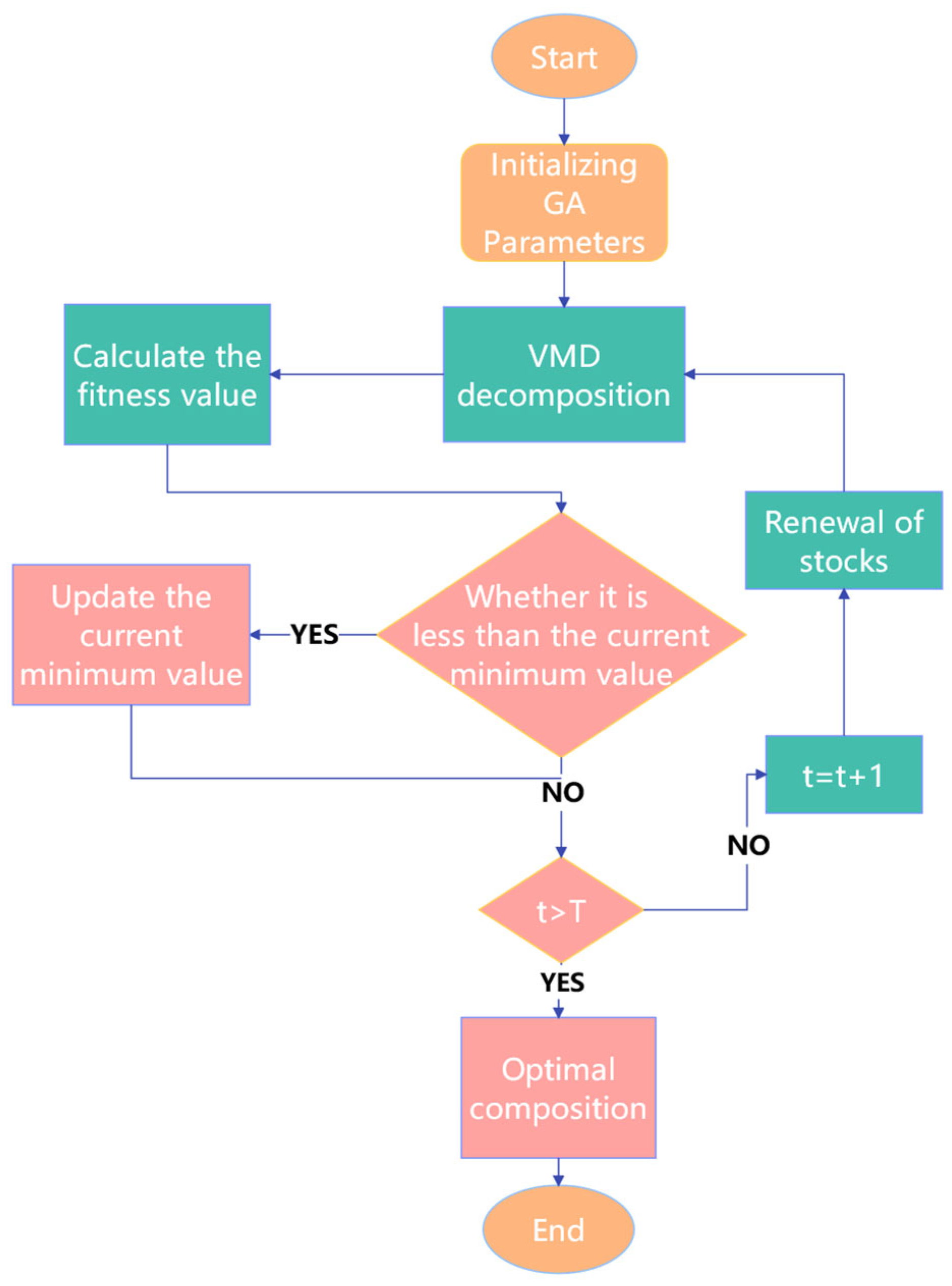
The flowchart of VMD parameter optimization using the GA is shown in Figure 1. First, initialize the population with decomposition level k encoded as integers and penalty factor α encoded as floating-point numbers, with the following value ranges: k ∈ [3, 11], α ∈ [300, 5000]. Next, perform VMD decomposition on the acquired signal to obtain IMF components, then calculate the fitness values for different parameter combinations (k, α). Subsequently, perform selection, crossover, and mutation operations. Determine whether the current (k, α) is smaller than the historical minimum value; if so, update the minimum value and record this combination. Check if the maximum iteration count has been reached. If not, repeat the previous steps until reaching the maximum iteration count of 50, then output the optimal parameter combination values.
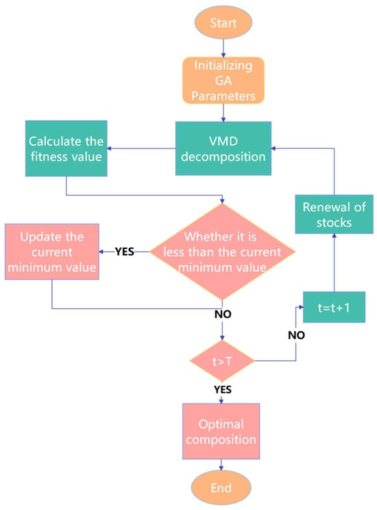
Figure 1.
Flowchart of VMD parameter optimization using the GA.
2.2. Parameter-Optimized Discrete Wavelet Transform Using Particle Swarm Optimization
The mathematical formulation of the DWT is expressed as follows:
where is the discrete wavelet coefficient at scale j and position k. x[n] is the original signal. is the discrete wavelet function derived from the mother wavelet u[n] through scaling and translation.
The correlation coefficients between each IMF component and the original signal under the optimal solution of the GA-optimized VMD are calculated, defined by the following formula:
where : correlation coefficient between signals x and y; E: expectation operator (Roman font); : mean values of signals x and y, respectively; : standard deviations of signals x and y, respectively. A value approaching 1 indicates a strong positive correlation between the two variables, demonstrating that most of the original signal’s fault characteristic information has been preserved. Conversely, a value closer to 0 suggests a weak correlation between them, meaning that little of the primary fault characteristic information from the original signal has been retained.
In this study, signals are classified as follows: are defined as useless signals and directly discarded; are categorized as partially useful signals and subjected to PSO-optimized DWT for secondary denoising; and are retained as useful signals. The denoising performance is evaluated using the minimum RMSE criterion, where smaller RMSE values indicate superior denoising. The RMSE is defined as follows:
Figure 2 illustrates the parameter optimization workflow for the Discrete Wavelet Transform (DWT) using particle swarm optimization (PSO). The algorithm proceeds through the following steps: initialize the particle swarm population; randomize particle velocities within predefined bounds; and define search space parameters: decomposition levels: L ∈ [1, 10] and wavelet basis functions: db, sym, coif, and bior families. The optimization procedure is as follows: perform DWT decomposition on selected signal components, compute RMSE as the fitness criterion for each parameter combination, and update particle velocities and positions according to PSO dynamics. The current RMSE value is compared with the historical minimum. If it is lower than the historical minimum, the minimum value is updated and the corresponding combination is recorded. The iteration continues until the maximum number of iterations (50) is reached, at which point the optimal combination is output.
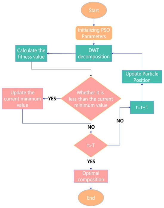
Figure 2.
Flowchart of PSO-optimized DWT parameters.
2.3. Signal Reconstruction Using the Parameter-Optimized VMD-DWT
The signal reconstruction process of VMD-DWT based on algorithm optimization is shown in Figure 3.
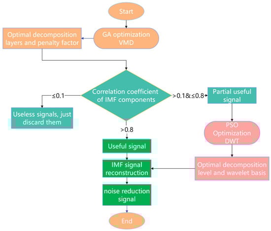
Figure 3.
Flowchart of algorithm-optimized VMD-DWT signal reconstruction process.
The processing flow is as follows: First, optimize VMD parameters using the genetic algorithm and calculate the of IMFs under optimal decomposition parameters. Then, discard IMFs with , and apply PSO-optimized DWT to IMFs with . Retain IMFs with for signal reconstruction. Finally, reconstruct the signal by combining DWT-denoised IMFs and retained IMFs with .
3. The Proposed Model
3.1. Network Model of CNN-BILSTM
3.1.1. CNN Theory
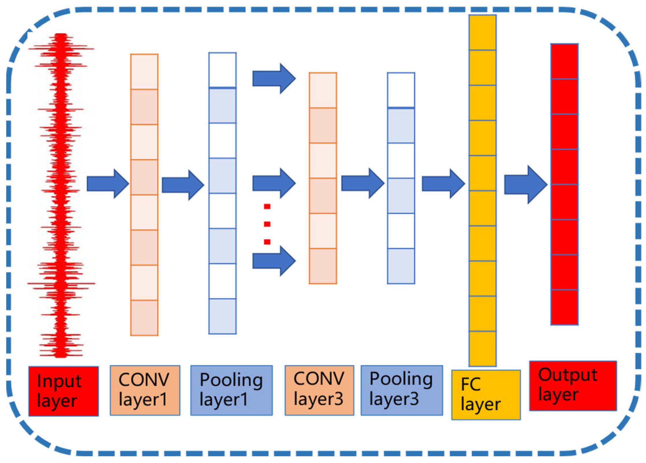
A CNN is a multi-layer neural network composed of an input layer, convolutional (CONV) layers, pooling layers, and fully connected (FC) layers. Its typical architecture is illustrated in Figure 4.

Figure 4.
CNN network architecture.
The CONV serves as the core component of CNN. Its primary function is to execute convolution operations on input data using convolutional kernels and propagate the resulting feature maps to the subsequent network layer. The convolution operation is mathematically expressed as follows:
In the above equation, represents the i-th feature at layer l, f denotes the non-linear activation function (e.g., ReLU), is the convolutional kernel weight matrix for the i-th filter at layer l, ∗ indicates the convolution operator, corresponds to the output from the (l − 1)-th layer, and is the bias term for the i-th channel at layer l.
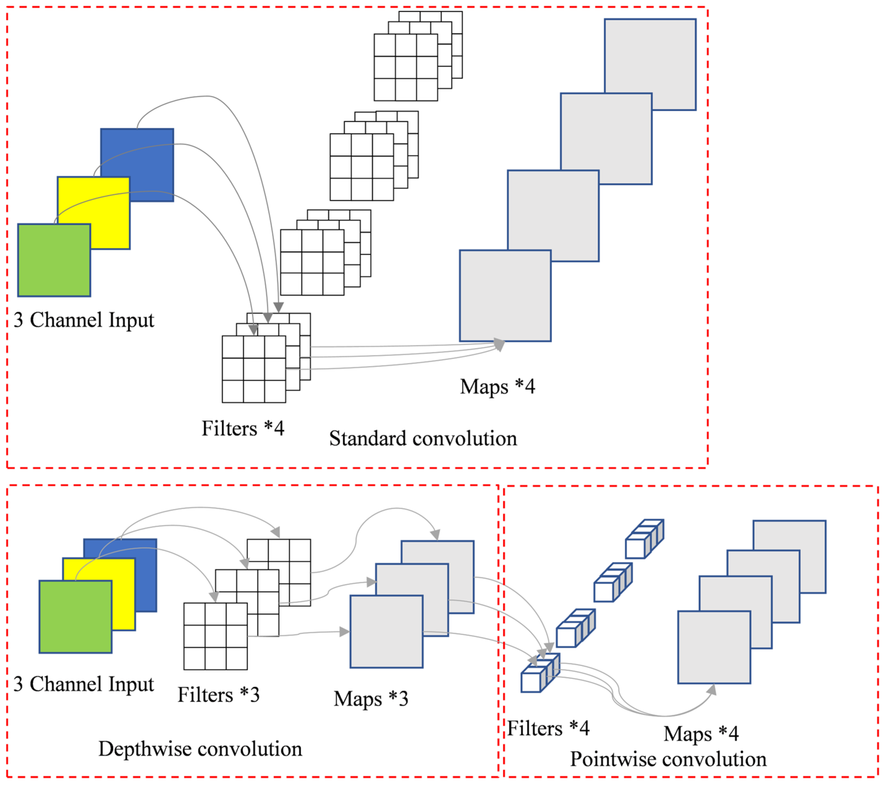
A depthwise separable convolution (dsc) comprises two sequential operations: depthwise convolution and pointwise convolution. The mathematical formulation of dsc is expressed as follows:
where , , denotes the number of input channels and k represents the convolution kernel size, is the bias of the depthwise convolution, , is the feature mapping matrix, denotes the number of output channels, and is the bias of the pointwise convolution. By decomposing the standard convolution into depthwise convolution (channel expansion) and 1 × 1 convolution, the computational complexity is reduced to of the original.
Figure 5 illustrates the schematic architecture of a depthwise separable convolution. Consider an input layer with three channels processed by a convolutional layer containing four filters, producing four output feature maps while maintaining identical spatial dimensions as the input. Parameter analysis reveals the following: Standard convolution: parameters = 4 filters × 3 input channels × 3 × 3 kernel = 108. Depthwise separable convolution: depthwise convolution: parameters = 3 channels × 3 × 3 kernel = 27. Pointwise convolution: parameters = 1 × 1 kernel × 3 input channels × 4 filters = 12. The total parameters are 39. This implementation achieves a 63.9% reduction in parameter count (39 vs. 108), demonstrating the computational efficiency of depthwise separable convolutions. The decomposed structure maintains equivalent input–output dimensionality while significantly decreasing model complexity.
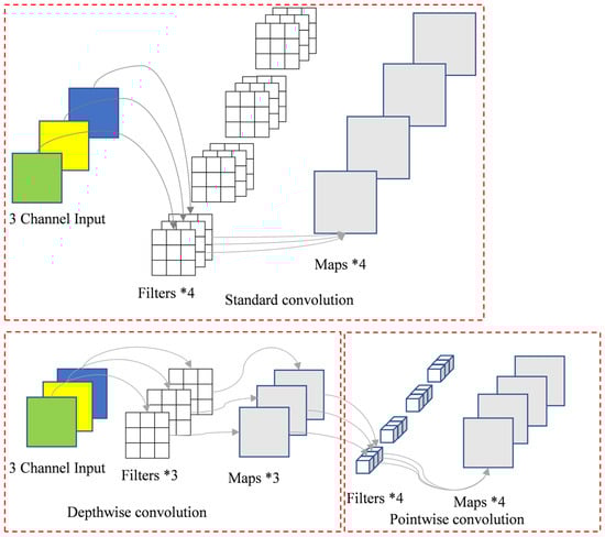
Figure 5.
Schematic diagram of depthwise separable convolution architecture.
3.1.2. BILSTM Theory
The BiLSTM neural network introduced in this study features two opposing-directional temporal outputs (denoted as for the forward network and for the backward network). The computational expressions for the forward and backward outputs are as follows:
the final output is a combined result of the forward and backward network outputs, which can be mathematically expressed as follows:
3.1.3. Hybrid Attention Theory
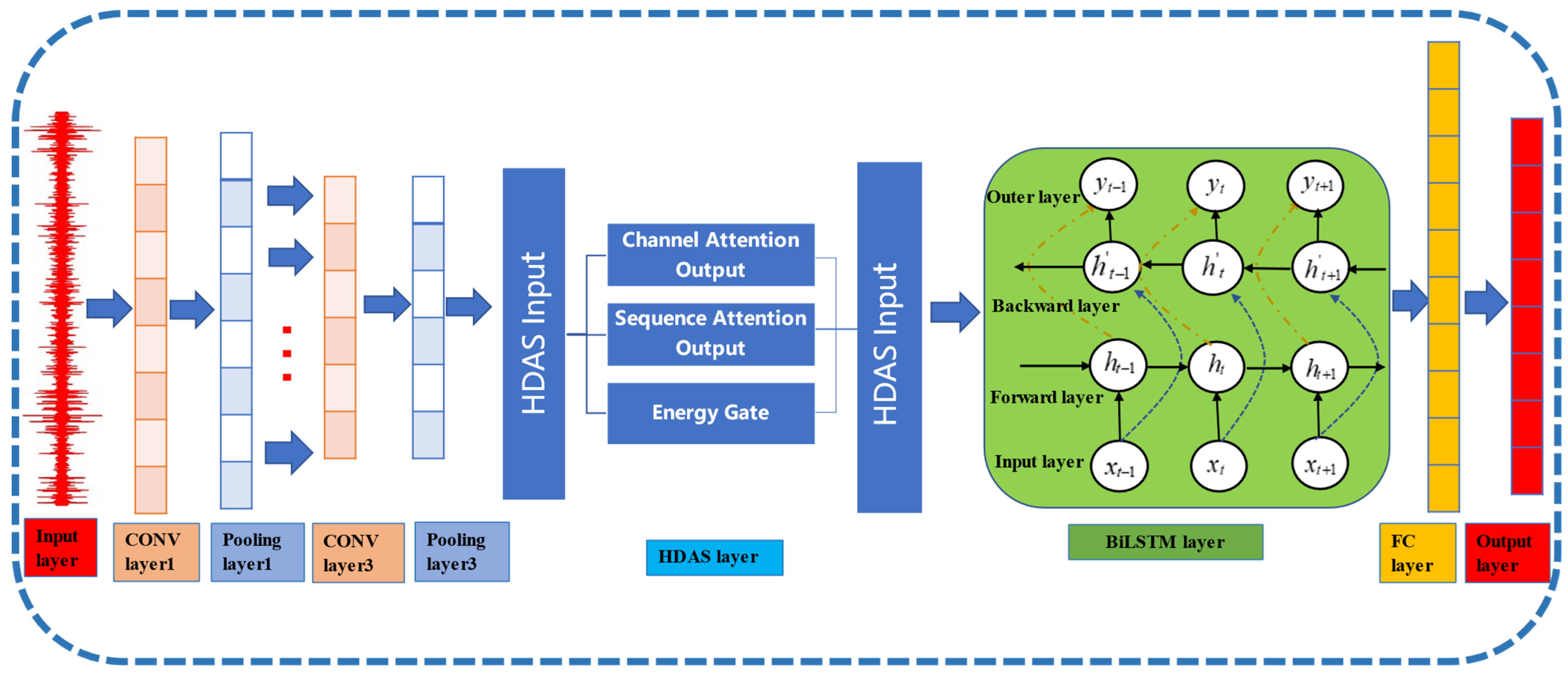
Hybrid attention dynamically fuses input features by integrating channel-wise features and spatial-temporal features. It consists of three components: channel attention, which quantifies the importance of different input channels; spatial attention, which captures local temporal correlations; and energy gating, which dynamically adjusts attention weights based on signal energy. Let the input feature tensor be denoted as , where N is the number of samples, C is the number of input channels, and T is the time series length. The channel attention module is structured as follows:
where GAP(X) denotes the global average pooling operation, yielding an output dimension of , and are the weight matrices of the first and second fully connected layers, respectively, and represents the Swish activation function, as follows:
The spatial attention module is the following:
where , 3 × 1 convolutional kernel weight matrix, and ∗ denotes the convolution operation. The energy gating mechanism is as follows:
where E represents the average energy vector along the time axis, 0.7 is an empirical coefficient to regulate gating sensitivity, and denotes the normalized energy gating vector. The final hybrid attention output is expressed as follows:
the output dimensionality is preserved as , enabling feature-weighted fusion.
3.1.4. HADS-CNN-BILSTM Structure
Combining the CNN architecture from Figure 4 with the theoretical descriptions of BiLSTM and hybrid attention provided in the text, the network structure of HADS-CNN-BiLSTM is illustrated in Figure 6.
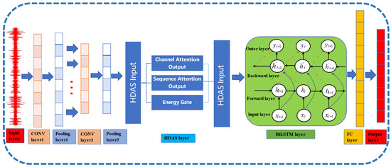
Figure 6.
Architecture of the HADS-CNN-BiLSTM network.
The feature propagation path of HADS-CNN-BiLSTM is as follows: input shape , processed by DSCNN to , hybrid attention processing to , BiLSTM processing to , and final output . Table 1 describes the dimensional transformations of feature matrices across different network layers.

Table 1.
The dimensional transformations of feature matrices across different network layers.
In the HADS-CNN-BiLSTM system, an exponentially decaying learning rate scheduler is employed, with its mathematical formulation defined as follows:
where (initial learning rate) is set to , (decay rate) is 0.95, and t denotes the training epoch starting from 0. A log-uniform sampling strategy within the range [3 × 10⁻⁴, 1 × 10⁻³] significantly enhances search efficiency compared to linear methods. Additionally, a two-stage progressive training strategy is introduced: Hyperparameter search phase: identifies optimal network configurations (e.g., kernel size, filters) and training policies by selecting the best-performing architecture from candidate models based on validation metrics. Precision fine-tuning phase: Fully trains the optimal architecture to maximize its diagnostic potential under limited computational resources.
3.2. Feature Extraction
The VMD-DWT-reconstructed signals, optimized by the proposed algorithm, undergo feature extraction with a sliding window of 512 data points per sample. For each sample, 15 time-domain features are computed. A total of 200 samples per bearing type are generated, constructing the feature dataset. The 15 feature parameters listed in Table 2 are utilized to build this dataset. The signal parameters are defined as follows: = signal mean value; = signal variance; = signal mean square value; = signal root mean square value; = signal maximum value; = signal minimum value; = signal peak value; = signal peak-to-peak value; = signal mean absolute amplitude; = signal skewness; = signal kurtosis; = signal waveform factor; = signal crest factor; = signal skewness factor; = signal kurtosis factor.
Table 2.
Definitions of feature formulas.
3.3. Technological Routine
The bearing fault diagnosis workflow based on the algorithm-optimized VMD-DWT and HADS-CNN-BiLSTM hybrid model is schematically illustrated in Figure 7.

Figure 7.
Fault diagnosis process.
Step 1: Collect vibration signals under different operational states of bearings.
Step 2: The vibration signal is first decomposed using VMD. The resulting IMF components are classified into three categories based on correlation coefficients: useless signals, partially useful signals, and useful signals. The partially useful signals undergo noise reduction via DWT, after which they are combined with the useful signals to reconstruct the final signal.
Step 3: Feature extraction was performed on the reconstructed signals to create a dataset. The dataset contains 200 samples for each of four bearing conditions, labeled as 0, 1, 2, and 3, respectively. The dataset was randomly divided into training and testing sets with a 7:3 ratio.
Step 4: Industrial-grade feature standardization is applied to the feature data to eliminate the influence of varying feature scales and suppress outlier interference.
Step 5: The processed data from Step 4 were fed into the HADS-CNN-BiLSTM model, which integrates a hybrid attention mechanism, depthwise separable convolution, and BiLSTM, to extract discriminative features and perform fault diagnosis.
Step 6: Classification labels are outputted to predict rolling bearing fault types.
4. Experimental Validation
In this section, the CWRU bearing dataset [29] is employed to validate the effectiveness of the proposed model, while the XJTU-SY dataset [30] is utilized to assess its generalization capability.
4.1. Case A: CWRU Datasets Experiment
4.1.1. Description of the CWRU Dataset
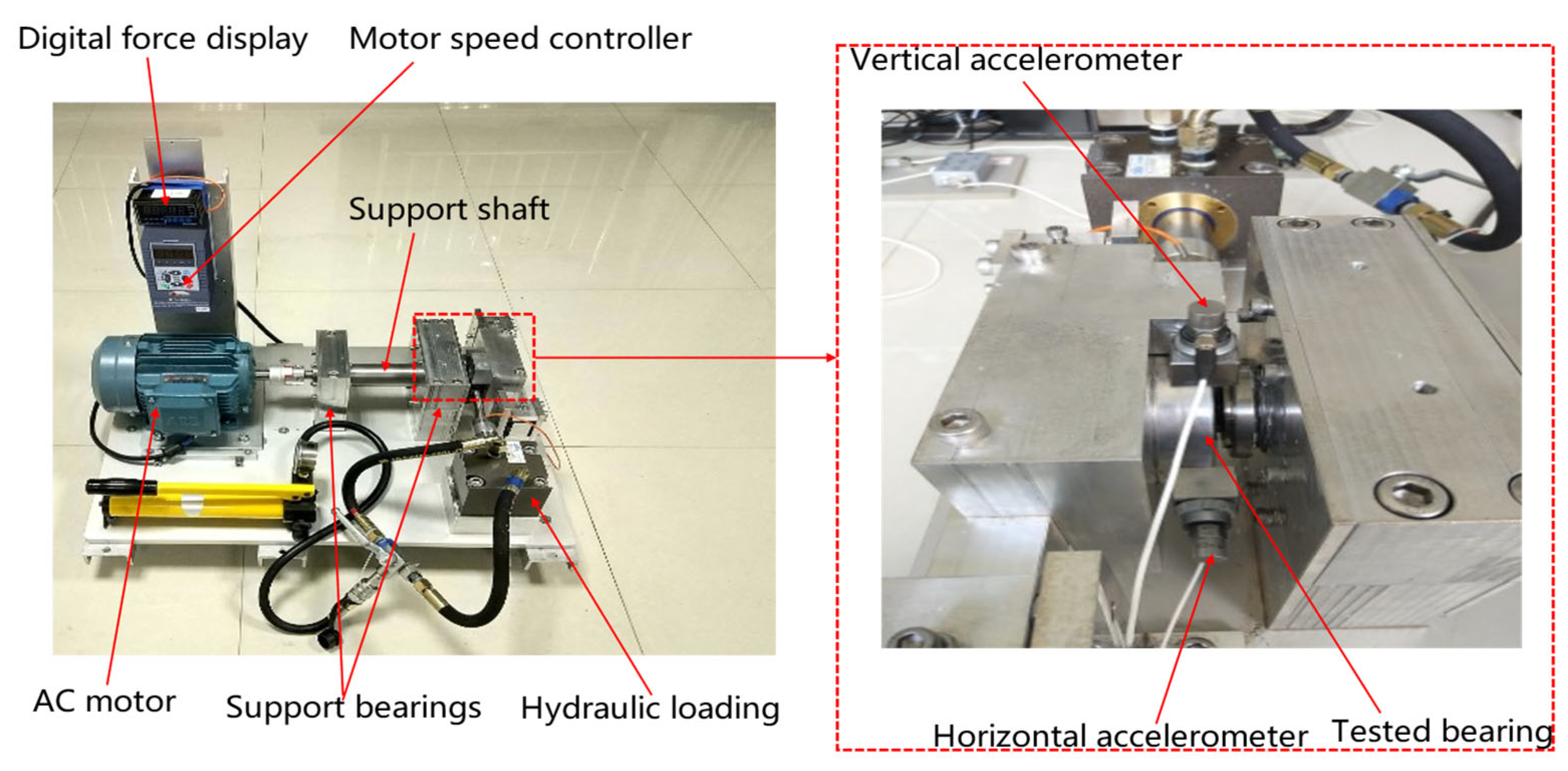
The dataset originates from the CWRU Bearing Data Center at Case Western Reserve University. The experiments focus on diagnosing motor drive-end bearings and fan-end bearings, covering four conditions: Normal Condition (NC), Inner Race Fault (IF), Outer Race Fault (OF), and Rolling Element Fault (RF). The fault diameters were 7 mils, 14 mils, 21 mils, and 28 mils (1 mil = 0.001 inches). The test bearings operated under four rotational speeds: 1730 rpm, 1750 rpm, 1772 rpm, and 1797 rpm. The bearing fault diagnosis test rig is illustrated in Figure 8.
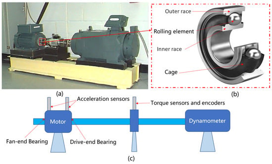
Figure 8.
(a) Test rig photo, (b) rolling bearing structure, and (c) test rig schematic.
This study utilizes vibration data from the drive-end bearing with a sampling frequency of 12 kHz, a rotational speed of 1730 rpm, and a fault diameter of 0.014 inches.
4.1.2. Signal Reconstruction
The GA-VMD method is sequentially applied to decompose signals from the Rolling Elements, Inner Race, Outer Race, and Normal Condition bearings, yielding the optimal decomposition level K and penalty factor α for each bearing state under VMD. The results are summarized in Table 3.
Table 3.
Optimal decomposition level k and penalty factor a for VMD decomposition.
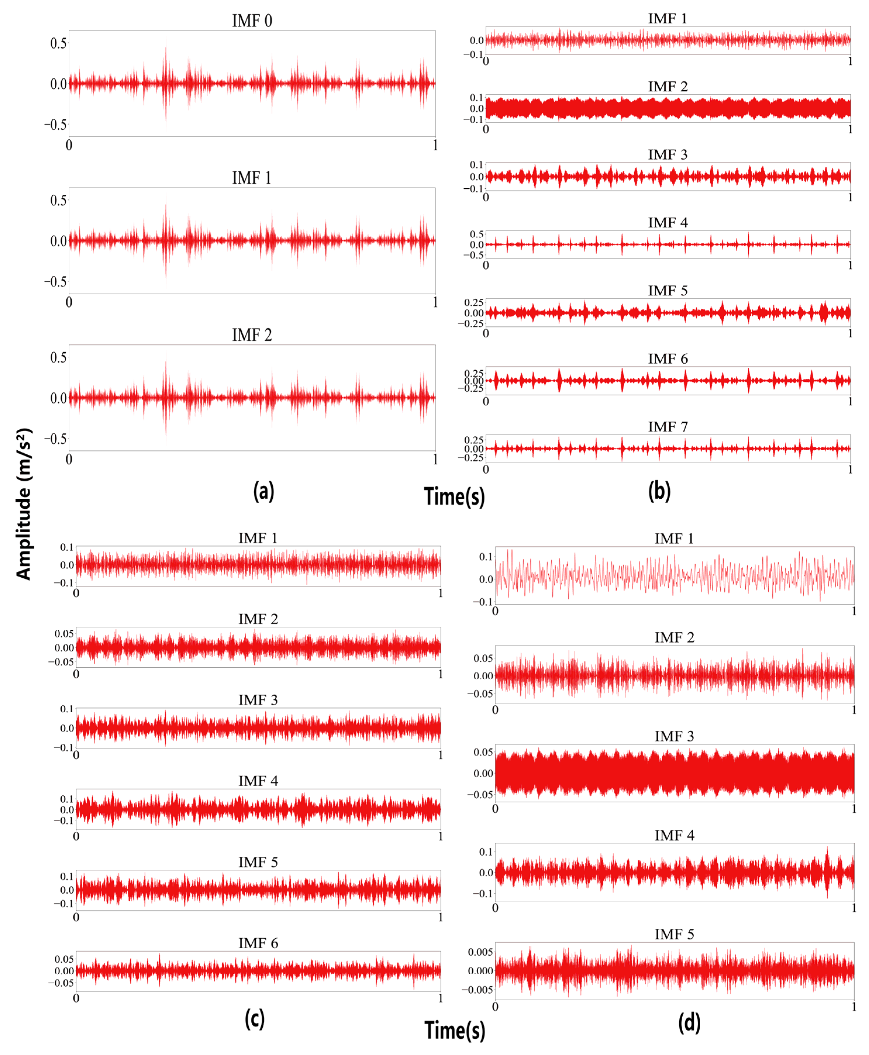
The time-domain waveforms of the IMFs derived from vibration signals under optimal VMD parameters are plotted and illustrated in Figure 9.

Figure 9.
After VMD decomposition: (a) RF, (b) IF, (c) OF, and (d) NC.
The correlation coefficients of the Intrinsic Mode Functions (IMFs) in Figure 8 are calculated and summarized in Table 4.
Table 4.
Correlation coefficients between IMFs and raw signals.
The optimal decomposition level (L) and wavelet basis functions (ψ), determined based on the minimum RMSE criterion, are summarized in Table 5.
Table 5.
Optimal decomposition Ψ and L.
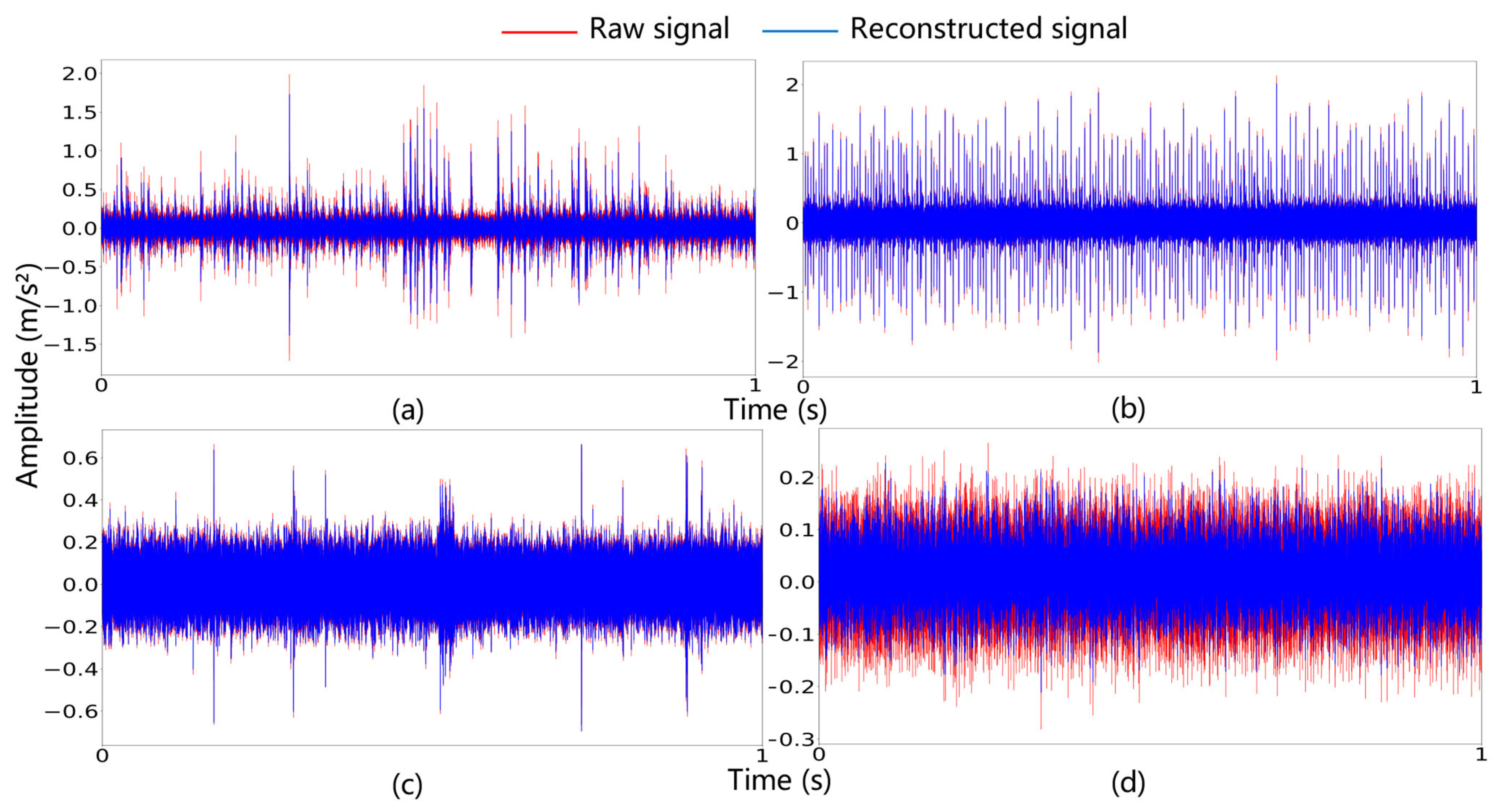
The time-domain waveforms of the reconstructed signals and raw signals are plotted in Figure 10. The reduced vibration amplitudes evident in the figure validate the method’s significant noise-suppression capability.
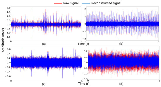
Figure 10.
Time-domain waveforms of raw and reconstructed signals: (a) RF, (b) IF, (c) OF, and (d) NC.
4.1.3. Bearing Fault Identification
In fault diagnosis, accuracy is defined as the ratio of correctly predicted samples (both true positives and true negatives) to the total number of samples, reflecting the model’s overall predictive capability. Recall (sensitivity) represents the proportion of actual positive samples correctly identified as positive by the model. Precision quantifies the proportion of true positive predictions among all samples predicted as positive. The F1 Score, a harmonic mean of precision and recall, provides a balanced evaluation of model performance. The mathematical expressions are defined as follows:
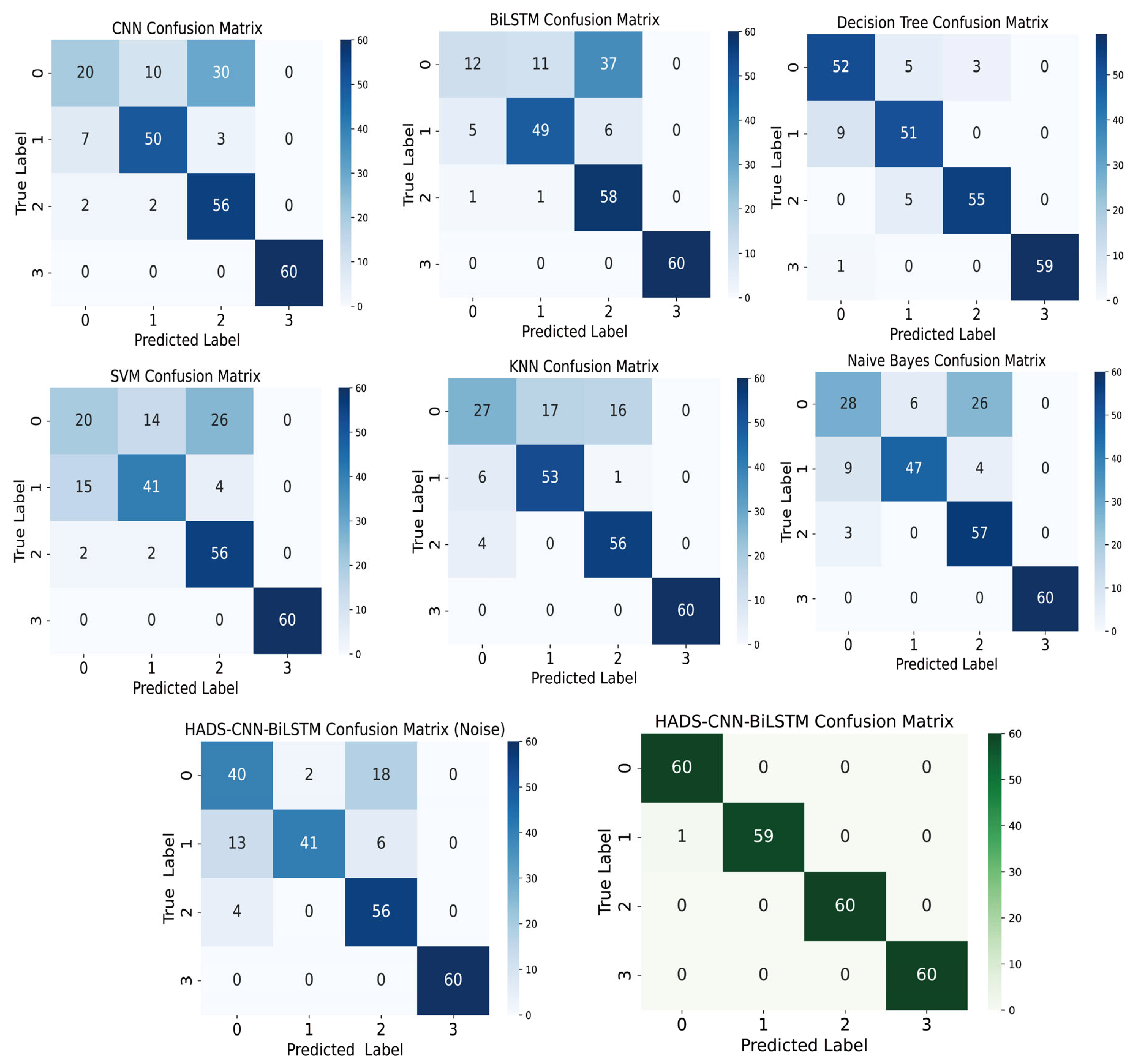
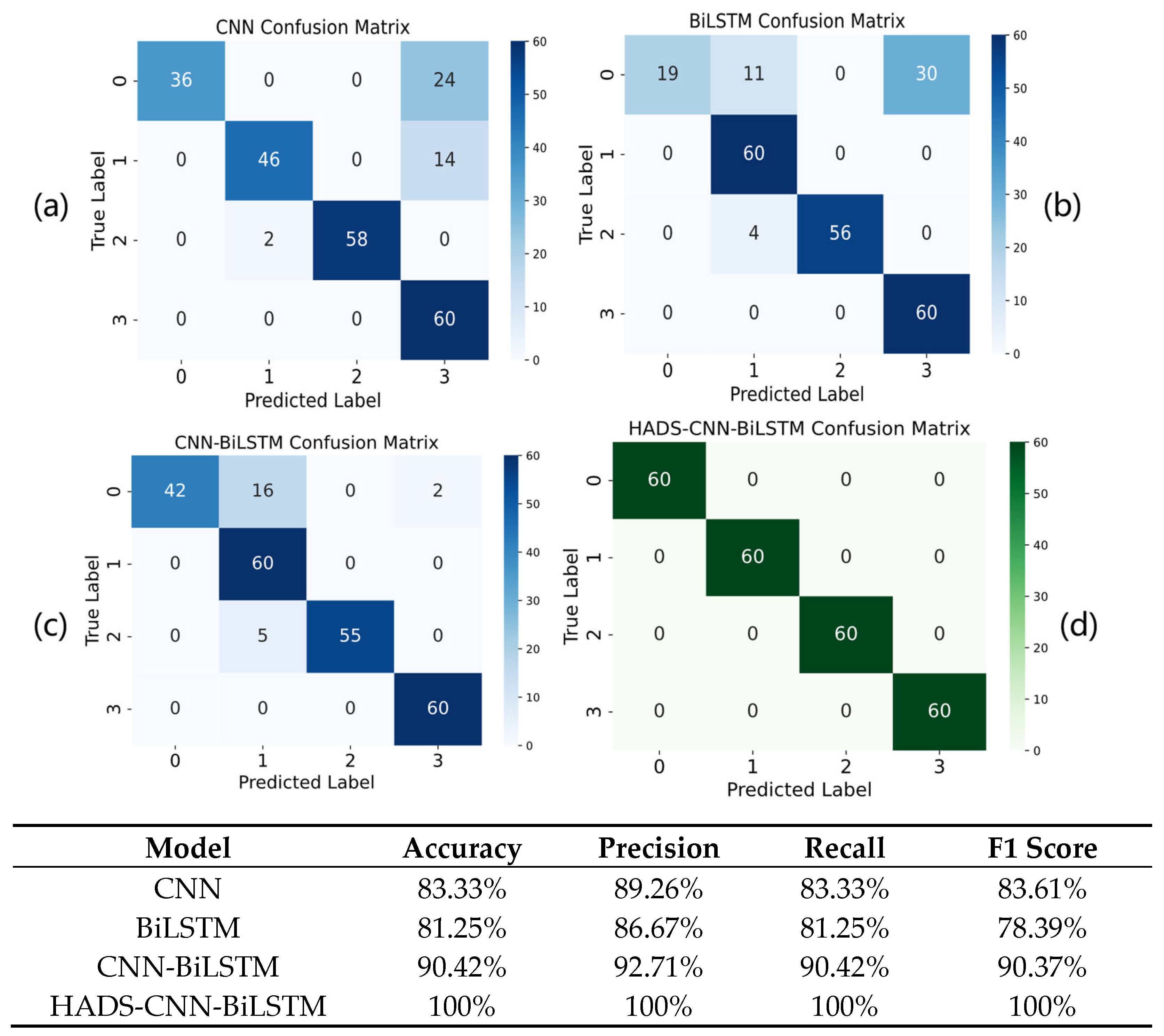
The reconstructed signals processed by VMD-DWT were fed into the HADS-CNN-BiLSTM model, which was then systematically replaced with standalone CNN, BiLSTM, and widely used comparative models (Decision Tree, SVM, KNN, and Naive Bayes) to validate the superiority of the proposed architecture. Concurrently, raw unprocessed data were directly input into the HADS-CNN-BiLSTM model to verify the effectiveness of the VMD-DWT signal reconstruction method. The confusion matrix results for all models are presented in Figure 11.
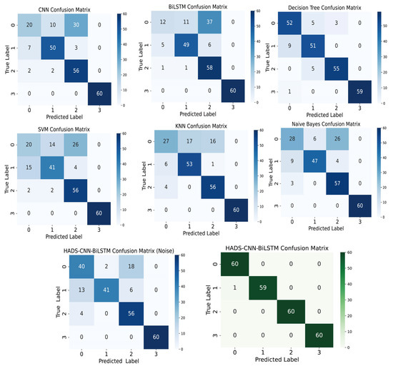
Figure 11.
Confusion matrix plot for CNN, BiLSTM, Decision Tree, SVM, KNN, Naive Bayes, HADS-CNN-BiLSTM (Noise), and HADS-CNN-BiLSTM models.
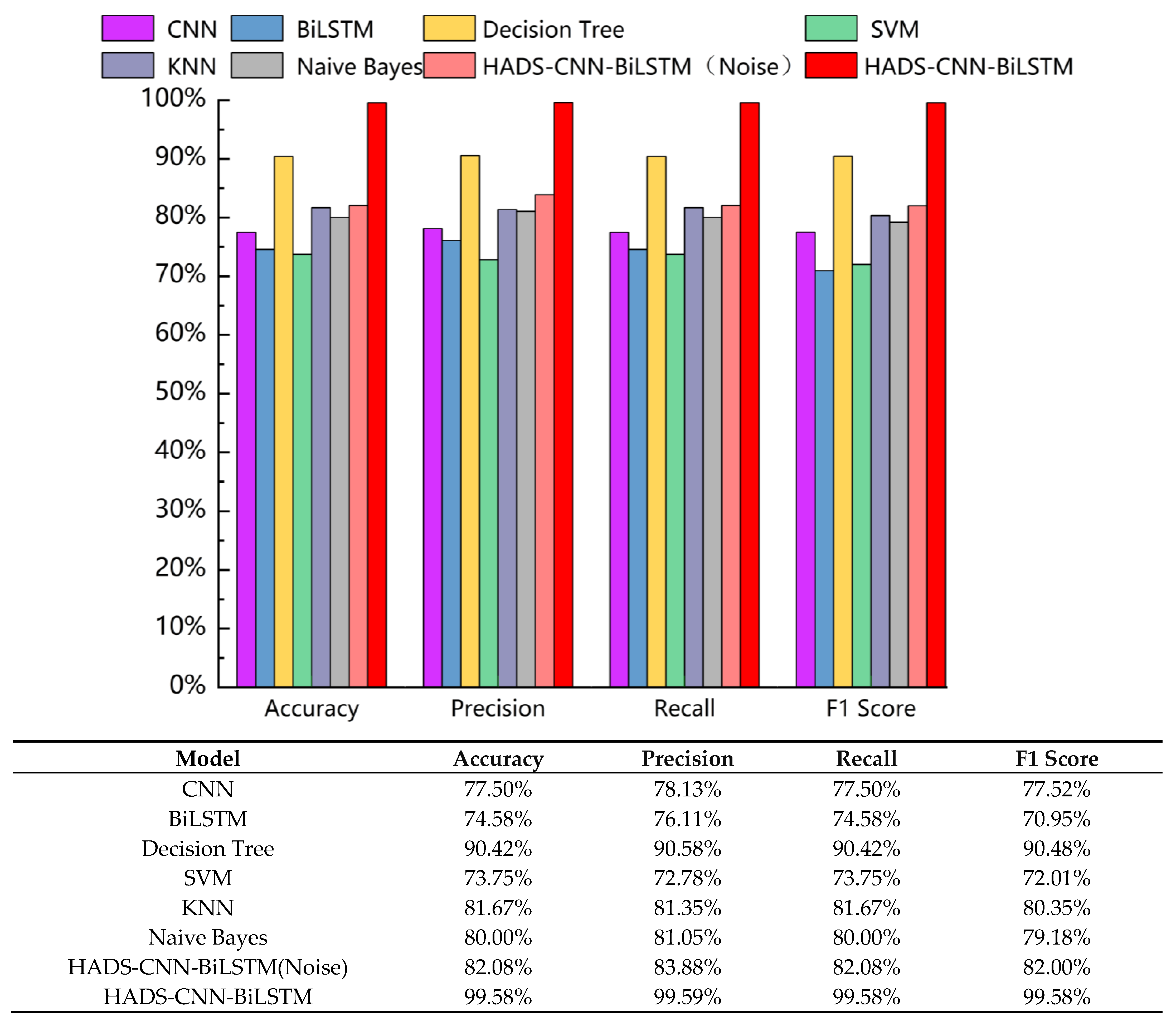
Based on the confusion matrices in Figure 11, the accuracy, precision, recall, and F1 Score of each model were calculated. The statistical results are summarized in Figure 12.

Figure 12.
The accuracy, precision, recall, and F1 Score of various models.
As shown in Figure 12, the HADS-CNN-BiLSTM model achieves superior performance in accuracy, precision, recall, and F1 Score compared to other models. When raw data without VMD-DWT joint denoising was directly input into the HADS-CNN-BiLSTM model, the accuracy, precision, recall, and F1 Score are 82.08%, 83.88%, 82.08%, and 82.00%. These results demonstrate that the diagnostic performance of the HADS-CNN-BiLSTM model deteriorates significantly when processing unprocessed raw data, highlighting the critical role of VMD-DWT noise reduction in improving fault detection reliability. Compared to the standalone CNN, the HADS-CNN-BiLSTM model improves accuracy by 22.08% and the F1 Score by 22.06%. Against the BiLSTM model, accuracy and the F1 Score are enhanced by 25% and 28.63%, respectively. Among the four conventional models (Decision Tree, SVM, KNN, and Naive Bayes), Decision Tree performs best, while SVM performs worst. The HADS-CNN-BiLSTM model surpasses Decision Tree by 9.16% in accuracy and 9.1% in F1 Score, and outperforms SVM by 25.83% in accuracy and 27.57% in F1 Score. This improvement is attributed to the VMD-DWT joint denoising method, which integrates time-domain and frequency-domain techniques to effectively suppress noise interference in feature signals. Furthermore, the HADS-CNN-BiLSTM model has stronger feature extraction and temporal modeling capabilities, enabling more effective handling of complex time-series data and enhancing fault diagnosis accuracy and efficiency.
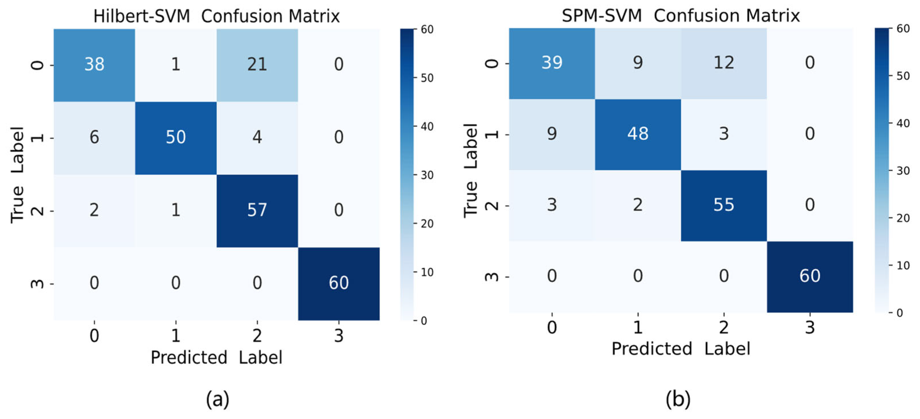
This study conducted comparative experiments on the original vibration data using two classical bearing fault diagnosis methods: Hilbert transform and the Shock Pulse Method (SPM). For the Hilbert transform approach, fault characteristic information was extracted from the envelope after transformation, including features such as envelope peak values, envelope kurtosis, and waveform complexity, which were then classified using SVM. The SPM method involved extracting shock pulse characteristics, including pulse amplitude, energy, and pulse count, followed by SVM classification. The classification results of these two classical methods are presented in Figure 13 below. As shown in Figure 13, the Hilbert-based method achieved an accuracy of 85.42%, while the SPM method reached 84.17%. Both traditional approaches demonstrated inferior performance compared to the proposed method in this study.
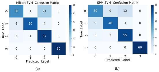
Figure 13.
Confusion matrix plot for (a) Hilbert-SVM and (b) SPM-SVM.
To ensure the statistical robustness of the HADS-CNN-BiLSTM model and mitigate potential randomness, the experimental data were validated through 10 independent trials. The mean values and variability of the diagnostic results across these trials are summarized in Table 6. As indicated by the results in Table 6, the HADS-CNN-BiLSTM model achieves average values exceeding 99.58% for accuracy, precision, recall, and F1 Score across all 10 experimental trials, demonstrating excellent diagnostic performance.
Table 6.
Diagnostic results under 10 experiments.
4.2. Case B: XJTU-SY Bearing Datasets Experiment
4.2.1. Description of the XJTU-SY Dataset
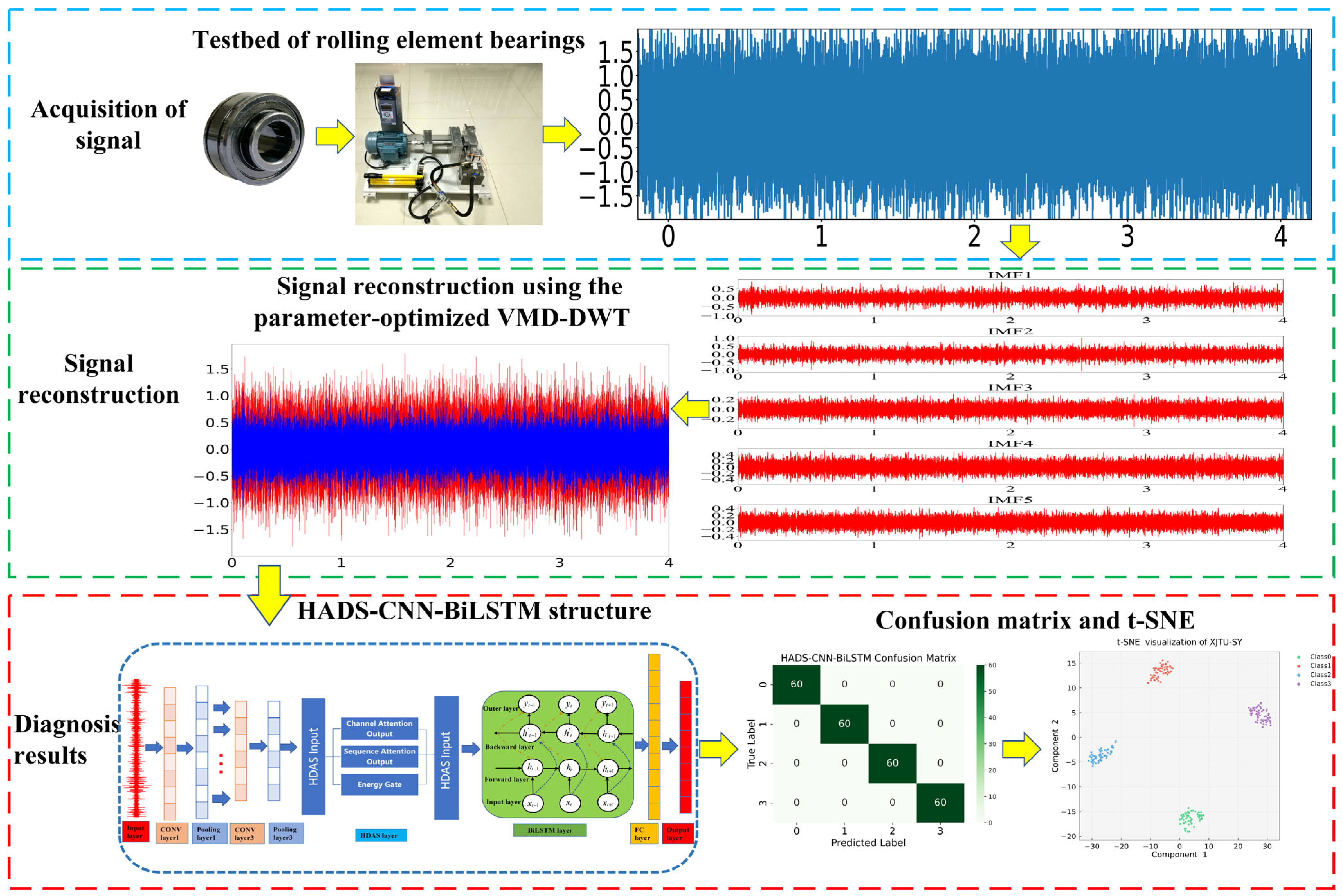
The XJTU-SY bearing datasets are provided by the Institute of Design Science and Basic Component at Xi’an Jiaotong University (XJTU), Xi’an, China. Two PCB 352C33 uniaxial accelerometers were mounted via magnetic bases on the horizontal and vertical directions of the test bearing to monitor four distinct operational modes: Normal Condition (NC), Inner Race Fault (IF), Outer Race Fault (OF), and Cage Fault (CF). The dataset encompassed three operational conditions with varying parameters: the first condition at 2100 rpm with a 12 kN radial load, the second at 2250 rpm with an 11 kN radial load, and the third at 2400 rpm with a 10 kN radial load. The bearing fault diagnosis test rig is illustrated in Figure 14. This study utilizes bearing data acquired under a sampling frequency of 25.6 kHz, rotational speed of 2250 rpm, and radial force of 11 KN.

Figure 14.
Testbed of Rolling Element bearings.
4.2.2. Signal Reconstruction
Processed using the same methodology, the time-domain waveforms of the algorithm-optimized VMD-DWT reconstructed signals and the raw signals were plotted. The signal reconstruction parameters of the optimized VMD-DWT algorithm are summarized in Table 7.
Table 7.
VMD-DWT signal reconstruction parameters optimized by algorithm.
Using the parameters listed in Table 7, the raw signals were reconstructed, and the time-domain waveforms of both the raw signals and the reconstructed signals are shown in Figure 15.
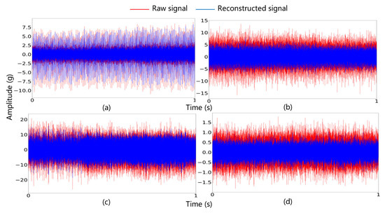
Figure 15.
Time-domain waveforms of raw and reconstructed signals: (a) IF, (b) CF, (c) OF, and (d) NC.
4.2.3. Bearing Fault Identification
The HADS-CNN-BiLSTM model is compared with CNN, BiLSTM, and CNN-BiLSTM models to further validate the effectiveness of the proposed method, with the results illustrated in Figure 16.
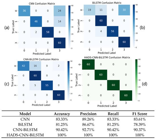
Figure 16.
Confusion matrix plot for (a) CNN, (b) BiLSTM, (c) CNN-BiLSTM, and (d) HADS-CNN-BiLSTM models.
As shown in Figure 16, the HADS-CNN-BiLSTM model achieves a 100% diagnostic accuracy rate on the XJTU-SY dataset. Compared to the standalone CNN, it improves accuracy by 16.67% and the F1 Score by 16.39%. Against the BiLSTM model, accuracy and the F1 Score are enhanced by 18.75% and 21.61%, respectively. When compared to the CNN-BiLSTM model, the HADS-CNN-BiLSTM demonstrates improvements of 9.58% in accuracy and 9.63% in the F1 Score.
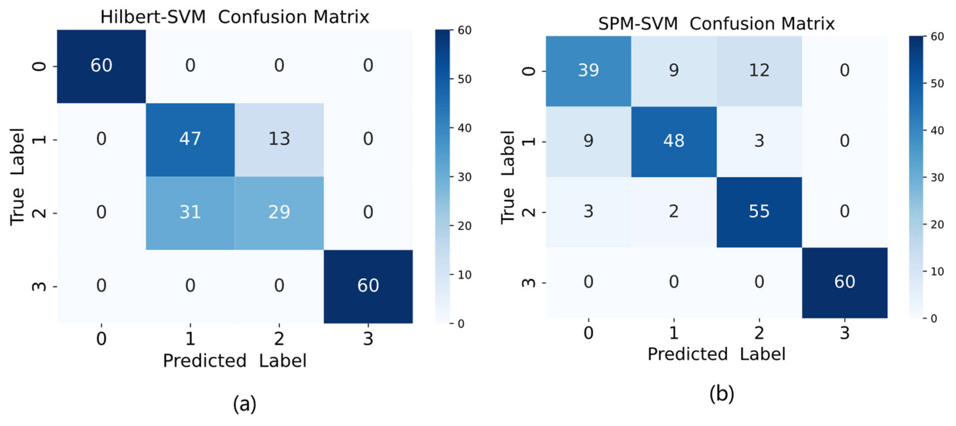
Consistent with the methodology described in Section 4.1.3, the XJTU-SY dataset was also evaluated using both Hilbert transform-based and SPM methods, with the comparative results presented in Figure 17. As shown in Figure 17, the Hilbert method achieved an accuracy of 81.67%, while the SPM method attained 77.5% accuracy, both demonstrating inferior performance compared to the proposed model in this study.

Figure 17.
Confusion matrix plot for (a) Hilbert-SVM and (b) SPM-SVM.
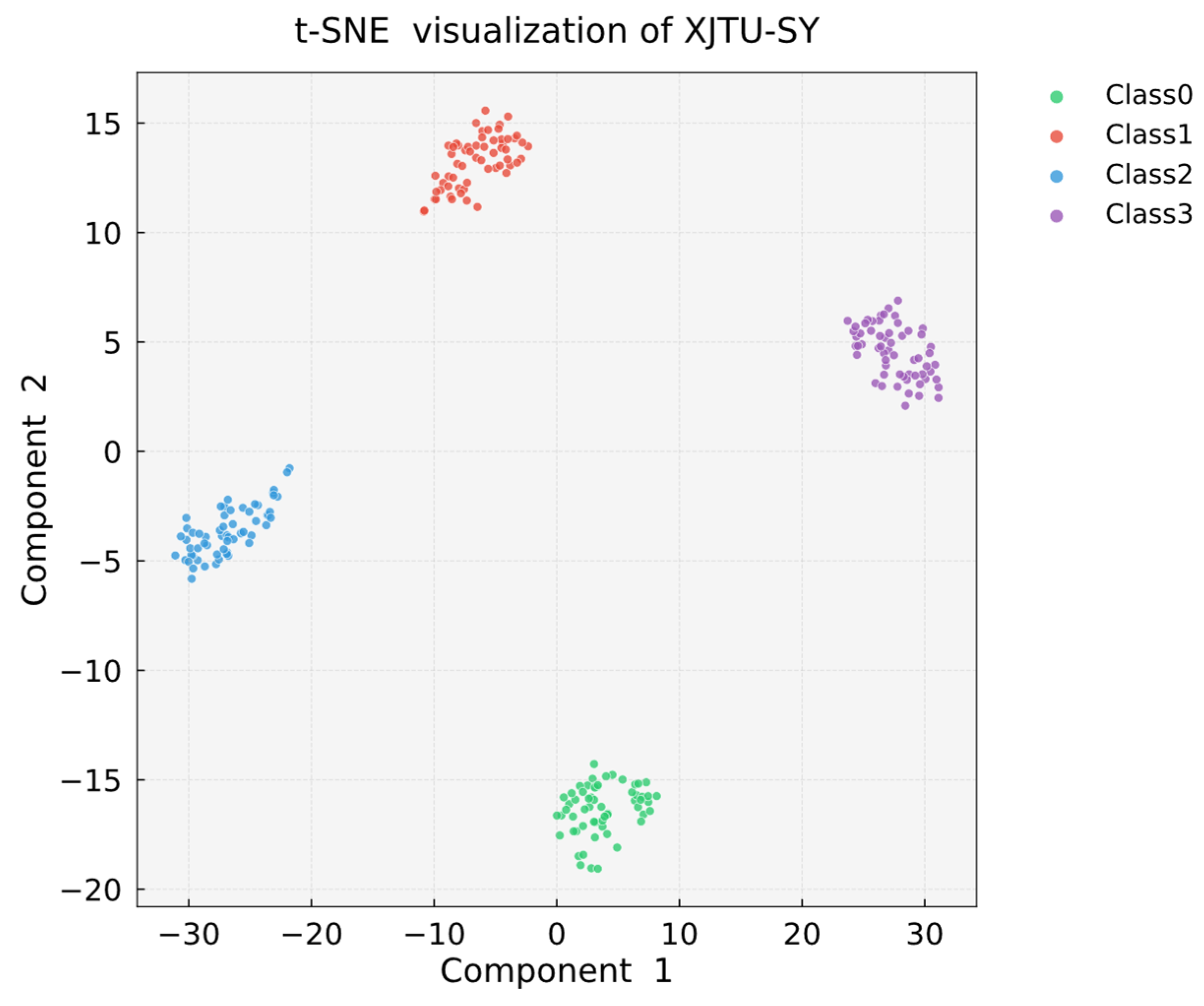
As demonstrated by the t-SNE visualization results in Figure 18, faults of the same category exhibit high intra-class clustering with distinct inter-class separation boundaries, further validating the robust performance of the proposed model on the XJTU-SY dataset.
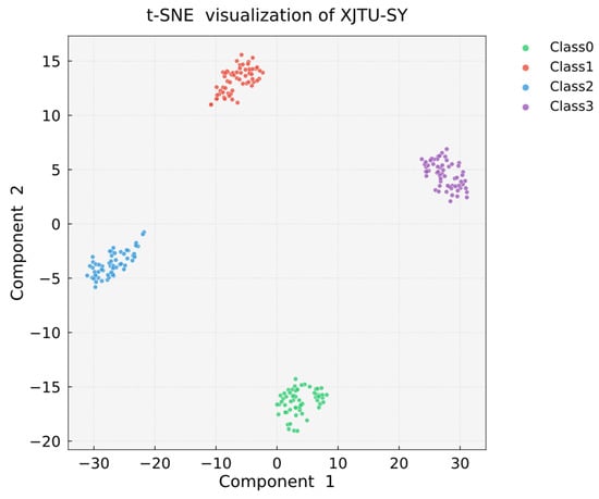
Figure 18.
T-SNE visualization of XJTU-SY.
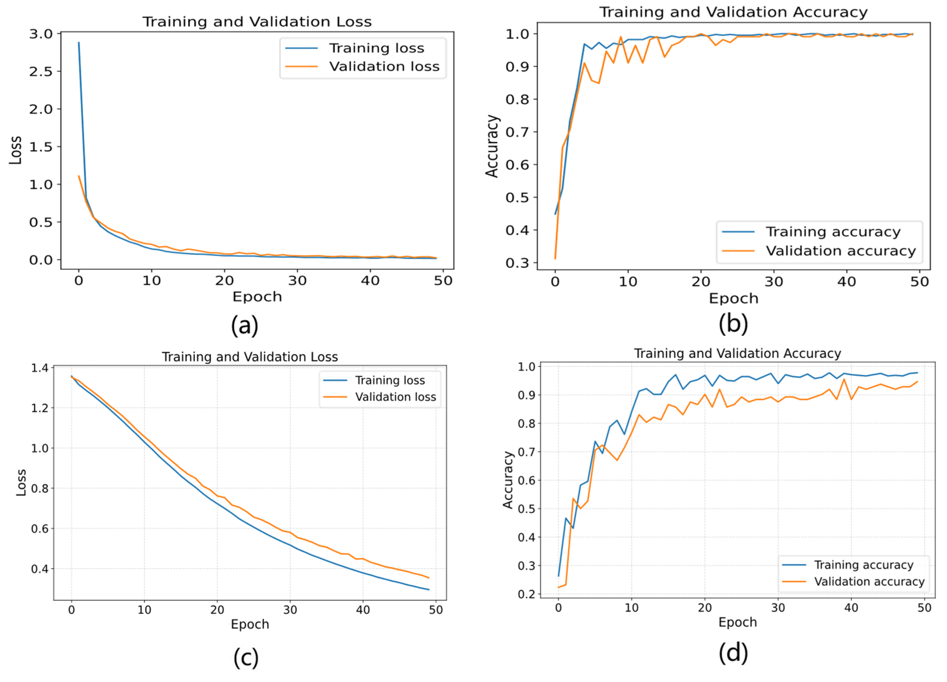
Using the denoised XJTU-SY dataset, the HADS-CNN-BiLSTM model was compared with and without dynamic learning rate scheduling and two-phase progressive training by plotting the loss variations and accuracy on both training and validation sets, demonstrating that these mechanisms accelerate convergence and improve model performance. As shown in Figure 19, panels (a) and (b) display the loss and accuracy curves for the model with dynamic learning rate scheduling and two-phase progressive training. After 30 epochs, the accuracy reached 100% on both training and validation sets and stabilized with further training, while the loss function also stabilized after 30 epochs. In contrast, panels (c) and (d) show that the model without these mechanisms achieved only about 90% accuracy after 30 epochs, and the loss function failed to converge even after 50 epochs. The results confirm that dynamic learning rate scheduling and two-phase progressive training effectively accelerate convergence and enhance model performance.
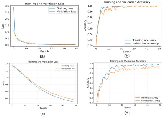
Figure 19.
Training curves with/without dynamic learning rate scheduling and two-stage progressive training: (a) loss (with), (b) accuracy (with), (c) loss (without), and (d) accuracy (without).
To validate the noise resistance performance of HADS-CNN-BiLSTM, noise resistance experiments were conducted. White noise of varying intensities was added to the original signals to generate contaminated signals, simulating vibration signals under different disturbance environments. The standard formula for calculating the SNR is defined as follows:
where is the signal power, is the noise power, is the signal amplitude, and is the noise amplitude. The formula indicates that a lower SNR value corresponds to less noise in the signal. White noise with SNR levels of −6 dB, −4 dB, −2 dB, 0 dB, and 2 dB was added to the original signals to generate five noisy datasets. Time-domain plots of the first 1024 vibration points under different SNR conditions are shown in Figure 20.
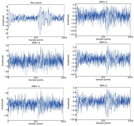
Figure 20.
Time-domain images with different SNRs.
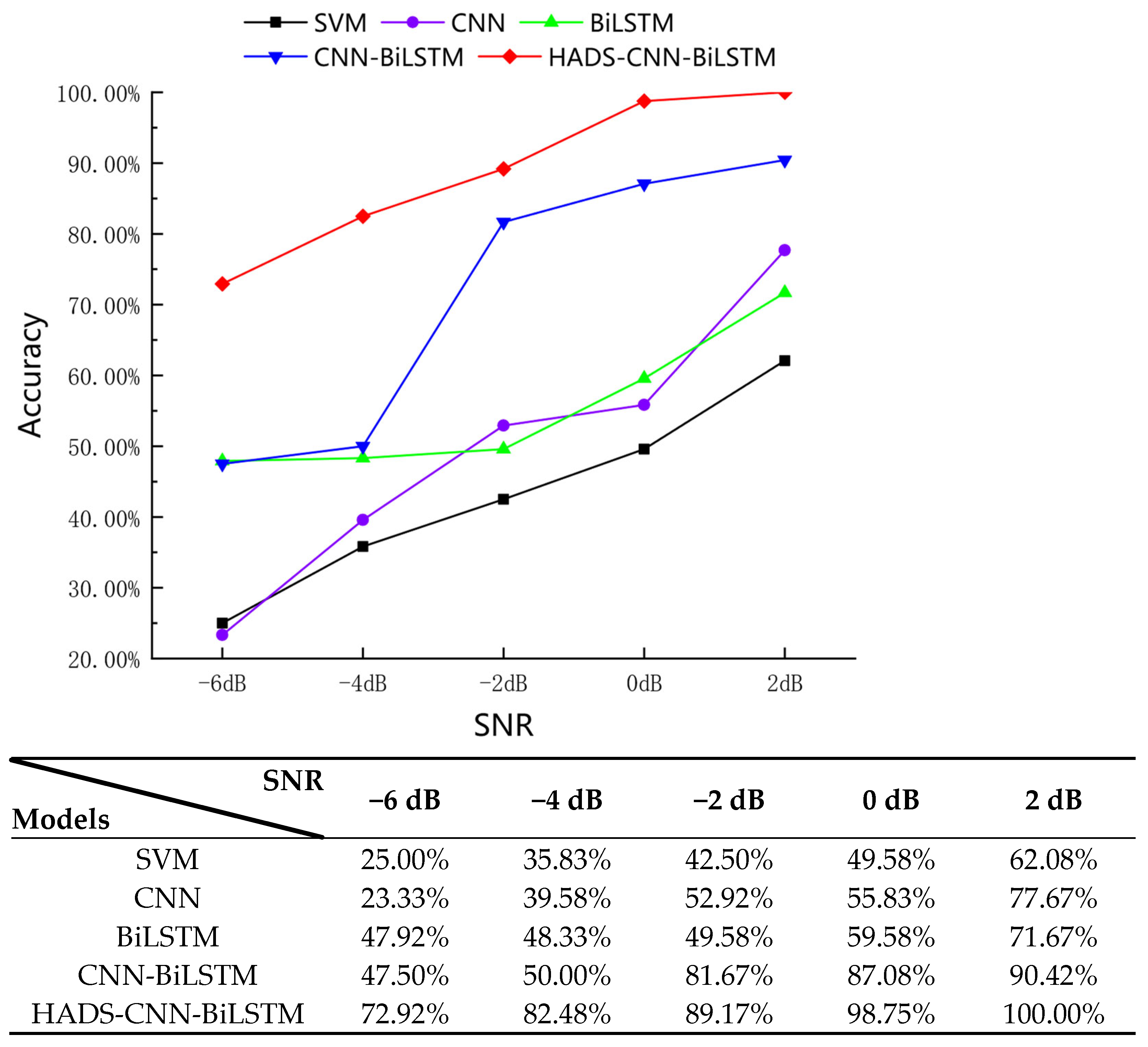
In noisy environments, certain characteristics of fault signals are obscured, increasing the difficulty of fault feature extraction. Comparative noise resistance experiments were conducted between the HADS-CNN-BiLSTM model and SVM, CNN, BiLSTM, and CNN-BiLSTM models. For each noisy dataset, experiments were repeated 10 times across all models, with the mean accuracy values from the 10 trials taken as the final results. The experimental outcomes are shown in Figure 21.
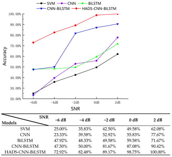
Figure 21.
Diagnostic accuracy of multiple models under varying SNR conditions.
As shown in Figure 21, the HADS-CNN-BiLSTM model demonstrates strong diagnostic accuracy across varying SNRs. At an SNR of −6 dB, the diagnostic accuracy of HADS-CNN-BiLSTM reaches 72.92%, significantly outperforming other comparable models. When the SNR increases to 2 dB, the accuracy achieves 100%. This improvement stems from the hybrid attention module, which integrates channel attention and spatial attention mechanisms to dynamically enhance critical fault features through energy gating. Compared to the static convolution in CNN-LSTM, it demonstrates superior noise suppression and adaptive feature weighting capabilities, indicating that the HADS-CNN-BiLSTM model, through its innovative integration of depthwise separable convolution, hybrid attention mechanisms, dynamic learning rate scheduling, and a two-stage progressive training strategy, delivers exceptional performance in fault diagnosis tasks.
5. Conclusions
A hybrid robust denoising method is proposed by integrating vibration signals processed through GA-optimized VMD and PSO-optimized DWT, effectively addressing the challenge of manual parameter selection in traditional VMD- and DWT-based signal denoising. This method synergizes time-domain and frequency-domain techniques to suppress noise interference on critical feature signals. Furthermore, the HADS-CNN-BiLSTM model is developed with innovative architectural designs to achieve multimodal feature fusion through a hybrid neural network. Key innovations include the following: (1) industrial-adapted depthwise separable convolution layers, which decompose standard convolution into depthwise convolution and 1 × 1 pointwise convolution to reduce computational complexity; (2) industrial-grade hybrid attention mechanisms that integrate channel-wise and spatiotemporal features, incorporating energy-based gating to dynamically adjust attention weights according to signal energy; and (3) optimized temporal modeling in BiLSTM through dynamic threshold gating units, where learnable threshold parameters autonomously regulate the activity of forget and input gates. Additionally, novel training strategies are implemented, including dynamic learning rate scheduling and a two-stage progressive training approach, enabling accelerated convergence and enhanced model performance.
The proposed method achieves fault diagnosis rates of 99.58% and 100% on the CWRU and XJTU-SY datasets, respectively. Experimental validation on these two public datasets confirms the model’s high generalization capability and robustness. Under strong noise interference conditions, comparative experiments with several common fault diagnosis models demonstrate the proposed method’s superior noise resistance.
Author Contributions
Conceptualization, L.S. and B.Z.; methodology, L.S.; software, L.S.; validation, L.S., B.Z. and X.K.; formal analysis, L.S.; investigation, L.S.; resources, B.Z.; data curation, L.S.; writing—original draft preparation, L.S.; writing—review and editing, B.Z.; visualization, L.S.; supervision, X.K.; project administration, B.Z.; funding acquisition, B.Z. All authors have read and agreed to the published version of the manuscript.
Funding
This study was funded by the Qinghai Province 2025 Key Research and Development and Transformation Plan Project (Grant No. 2025-QY-209).
Data Availability Statement
The data used in this study were sourced from publicly available datasets, and the methodology for accessing and obtaining these data resources has been thoroughly described in the manuscript.
Conflicts of Interest
The authors declare that they have no conflicts of interest.
References
- Fu, G.H.; Wei, Q.J.; Yang, Y.S.; Li, C.F. Bearing fault diagnosis based on CNN-BiLSTM and residual module. Meas. Sci. Technol. 2023, 34, 125050. [Google Scholar] [CrossRef]
- Wu, C.M.; Zheng, S.P. Fault Diagnosis Method of Rolling Bearing Based on MSCNN-LSTM. Comput. Mater. Contin. 2024, 79, 4395–4411. [Google Scholar] [CrossRef]
- Liang, P.F.; Wang, W.H.; Yuan, X.M.; Liu, S.Y.; Zhang, L.J.; Cheng, Y.W. Intelligent fault diagnosis of rolling bearing based on wavelet transform and improved ResNet under noisy labels and environment. Eng. Appl. Artif. Intell. 2022, 115, 105269. [Google Scholar] [CrossRef]
- Fernandes, M.; Corchado, J.M.; Marreiros, G. Machine learning techniques applied to mechanical fault diagnosis and fault prognosis in the context of real industrial manufacturing use-cases: A systematic literature review. Appl. Intell. 2022, 52, 14246–14280. [Google Scholar] [CrossRef]
- Yan, G.X.; Chen, J.; Bai, Y.; Yu, C.Q.; Yu, C.M. A Survey on Fault Diagnosis Approaches for Rolling Bearings of Railway Vehicles. Processes 2022, 10, 724. [Google Scholar] [CrossRef]
- He, Y.C.; Fang, H.S.; Luo, J.Q.; Pang, P.F.; Yin, Q. A hybrid method for fault diagnosis of rolling bearings. Meas. Sci. Technol. 2024, 35, 125012. [Google Scholar] [CrossRef]
- Wang, Z.; Xu, X.; Song, D.; Zheng, Z.; Li, W. A Novel Bearing Fault Diagnosis Method Based on Improved Convolutional Neural Network and Multi-Sensor Fusion. Machines 2025, 13, 216. [Google Scholar] [CrossRef]
- Tian, Y.L.; Liu, X.Y. A Deep Adaptive Learning Method for Rolling Bearing Fault Diagnosis Using Immunity. Tsinghua Sci. Technol. 2019, 24, 750–762. [Google Scholar] [CrossRef]
- Qin, A.S.; Mao, H.L.; Hu, Q. Cross-domain fault diagnosis of rolling bearing using similar features-based transfer approach. Measurement 2021, 172, 108900. [Google Scholar] [CrossRef]
- Wang, X.Q.; Li, Y.F.; Rui, T.; Zhu, H.J.; Fei, J.C. Bearing fault diagnosis method based on Hilbert envelope spectrum and deep belief network. J. Vibroeng. 2015, 17, 1295–1308. [Google Scholar]
- Zhang, X.H.; Zhao, J.M.; Kang, J.S.; Li, H.P.; Teng, H.Z. Bearing prognostics with non-trendable behavior based on shock pulse method and frequency analysis. J. Vibroeng. 2014, 16, 3963–3976. [Google Scholar]
- Geraei, H.; Rodriguez, E.A.V.; Majma, E.; Habibi, S.; Al-Ani, D. A Noise Invariant Method for Bearing Fault Detection and Diagnosis Using Adapted Local Binary Pattern (ALBP) and Short-Time Fourier Transform (STFT). IEEE Access 2024, 12, 107247–107260. [Google Scholar] [CrossRef]
- Wang, H.X.; Zhu, H.; Li, H.F. Multi-Mode Data Generation and Fault Diagnosis of Bearings Based on STFT-SACGAN. Electronics 2023, 12, 1910. [Google Scholar] [CrossRef]
- Qi, B.W.; Li, Y.Y.; Yao, W.; Li, Z.B. Application of EMD Combined with Deep Learning and Knowledge Graph in Bearing Fault. J. Signal Process. Syst. 2023, 95, 935–954. [Google Scholar] [CrossRef]
- Taibi, A.; Touati, S.; Aomar, L.; Ikhlef, N. Bearing fault diagnosis of induction machines using VMD-DWT and composite multiscale weighted permutation entropy. Compel 2024, 43, 649–668. [Google Scholar] [CrossRef]
- Li, J.N.; Luo, W.G.; Bai, M.S.; Song, M.K. Fault diagnosis of high-speed rolling bearing in the whole life cycle based on improved grey wolf optimizer-least squares support vector machines. Digit. Signal Process. 2024, 145, 104345. [Google Scholar] [CrossRef]
- Liu, D.D.; Cui, L.L.; Wang, G.; Cheng, W.D. Interpretable domain adaptation transformer: A transfer learning method for fault diagnosis of rotating machinery. Struct. Health Monit. 2025, 24, 1187–1200. [Google Scholar] [CrossRef]
- Yu, Y.J.; Zhao, X.Z.; Yu, C.F. Wavelet-Based Time-Reassigned Synchroextracting Transform with Application to Fault Diagnosis of Flexible Thin-Wall Bearing. IEEE T Instrum. Meas. 2023, 72, 3524412. [Google Scholar] [CrossRef]
- Lu, J.T.; Yin, Q.T.; Li, S.M. Rolling Bearing Composite Fault Diagnosis Method Based on Enhanced Harmonic Vector Analysis. Sensors 2023, 23, 5115. [Google Scholar] [CrossRef]
- Briglia, G.; Immovilli, F.; Cocconcelli, M.; Lippi, M. Bearing Fault Detection and Recognition From Supply Currents with Decision Trees. IEEE Access 2024, 12, 12760–12770. [Google Scholar] [CrossRef]
- Wang, B.; Qiu, W.T.; Hu, X.; Wang, W. A rolling bearing fault diagnosis technique based on recurrence quantification analysis and Bayesian optimization SVM. Appl. Soft Comput. 2024, 156, 111506. [Google Scholar] [CrossRef]
- Maincer, D.; Benmahamed, Y.; Mansour, M.; Alharthi, M.; Ghonein, S.S.M. Fault Diagnosis in Robot Manipulators Using SVM and KNN. Intell. Autom. Soft Co. 2023, 35, 1957–1969. [Google Scholar] [CrossRef]
- Sun, W.R.; Ma, Y.J.; Wang, R.L. k-NN attention-based video vision transformer for action recognition. Neurocomputing 2024, 574, 127256. [Google Scholar] [CrossRef]
- Peretz, O.; Koren, M.; Koren, O. Naive Bayes classifier-An ensemble procedure for recall and precision enrichment. Eng. Appl. Artif. Intell. 2024, 136, 108972. [Google Scholar] [CrossRef]
- Ni, Z.; Tong, Y.F.; Song, Y.X.; Wang, R.K. Enhanced Bearing Fault Diagnosis in NC Machine Tools Using Dual-Stream CNN with Vibration Signal Analysis. Processes 2024, 12, 1951. [Google Scholar] [CrossRef]
- Chen, H.M.; Meng, W.; Li, Y.J.; Xiong, Q. An anti-noise fault diagnosis approach for rolling bearings based on multiscale CNN-LSTM and a deep residual learning model. Meas. Sci. Technol. 2023, 34, 045013. [Google Scholar] [CrossRef]
- Han, K.X.; Wang, W.H.; Guo, J. Research on a Bearing Fault Diagnosis Method Based on a CNN-LSTM-GRU Model. Machines 2024, 12, 927. [Google Scholar] [CrossRef]
- Xu, H.; Xiao, Y.C.; Sun, K.; Cui, L.L. Improved Depthwise Separable Convolution for Transfer Learning in Fault Diagnosis. IEEE Sens. J. 2024, 24, 33606–33613. [Google Scholar] [CrossRef]
- Smith, W.A.; Randall, R.B. Rolling element bearing diagnostics using the Case Western Reserve University data: A benchmark study. Mech. Syst. Signal Process. 2015, 64–65, 100–131. [Google Scholar] [CrossRef]
- Wang, B.; Lei, Y.G.; Li, N.P.; Li, N.B. A Hybrid Prognostics Approach for Estimating Remaining Useful Life of Rolling Element Bearings. IEEE T Reliab. 2020, 69, 401–412. [Google Scholar] [CrossRef]


Disclaimer/Publisher’s Note: The statements, opinions and data contained in all publications are solely those of the individual author(s) and contributor(s) and not of MDPI and/or the editor(s). MDPI and/or the editor(s) disclaim responsibility for any injury to people or property resulting from any ideas, methods, instructions or products referred to in the content. |
© 2025 by the authors. Licensee MDPI, Basel, Switzerland. This article is an open access article distributed under the terms and conditions of the Creative Commons Attribution (CC BY) license (https://creativecommons.org/licenses/by/4.0/).