Feasibility Assessment of Novel Multi-Mode Camshaft Design Through Modal Analysis

Abstract

Camshafts in internal combustion engines are critical components not only for mechanical functionality but also for dynamic performance and vibration characteristics. This study aims to present a comprehensive modal analysis of the camshaft by integrating both computational and experimental approaches, followed by the design of an innovative multi-mode camshaft mechanism that enhances fuel efficiency and optimizes engine performance. First, a computational model of the camshaft is built with a proper mesh structure with a mesh size of 2 mm. Modal analysis is performed on the computational model, and the critical modal parameters of the camshaft are obtained. Second, modal tests are performed on the camshaft, which reveal an error of 15% on the computationally predicted natural frequencies. Third, a model updating procedure is applied to improve the accuracy of the computational model. The critical material properties are determined based on a sensitivity analysis, and the structural optimization process is performed accordingly. The optimized model solution is compared to the experimental data, and the computational model is validated based on both natural frequencies and mode shapes. The comparison of experimentally and computationally estimated natural frequencies reveal a difference below 2%. Mode shapes are compared based on Modal Assurance Criteria (MAC), and it is determined that the values of the elements in the main diagonal of the MAC matrix are around 0.9. Finally, the validated model is used as a basis for an innovative camshaft mechanism. The proposed mechanism offers enhanced flexibility by integrating multiple valve actuation methods, including Variable Valve Timing (VVT), Variable Valve Lift (VVL), Variable Valve Duration (VVD), Cylinder Deactivation, and Skip Cycle methods into a single camshaft for the first time in the literature. Modal analysis is performed on the proposed multi-mode design, and it is observed that the modified design resembles the modal properties of the original design.

1. Introduction

Valve control mechanisms play a crucial role in improving engine efficiency and fuel economy. Generally, the main focus of valve control studies is to overcome the limitations caused by constant operating conditions throughout the speed range of the engine, both at part and full load operating regimes. In conventional valvetrains, the kinematic relationships among the valve, camshaft, and crankshaft limits the flexibility in controlling the combustion phenomena. Although some modern valve control mechanisms have provided additional flexibility in valve operations, existing engine designs and previous works in the literature are conducted to evaluate individual applications of valve control strategies; such as Variable Valve Timing (VVT), Variable Valve Lift (VVL), Variable Valve Duration (VVD), Cylinder Deactivation (CDA), and Skip Cycle (SC) as well as only limited combinations of these strategies, such as CDA with VVT or VVL with VVT [1,2,3,4,5,6,7,8,9,10,11,12]. The proposed mechanism integrates all of these strategies (or valve control methods) to reduce fuel consumption into a single camshaft, presenting a more comprehensive and unified approach.

Integrating multiple functionalities into a single camshaft structure may introduce new loading conditions and vibration scenarios that can significantly influence the system’s dynamic behavior. Therefore, a comprehensive modal analysis is required to prevent local resonances, ensure mechanical integrity, and prove the accuracy of the mechanism under advanced engine control strategies.

The finite element method (FEM) is a powerful numerical technique used for solving complex engineering problems, and it is widely used to investigate modal parameters, which accurately reflect the dynamic properties of a given system. The finite element method provides significant flexibility in predicting dynamic and structural properties, such as natural frequencies, mode shapes, and stress distributions. However, any FEM-based computational model requires experimental validation [13]. Therefore, methods such as experimental modal analysis (EMA) are critical to ensure the reliability of FEM models by verifying and refining computational predictions.

Model updating is used as a systematic approach to improve the accuracy of FEM models and to minimize discrepancies between computational predictions and experimental results. The primary objective of model updating is to minimize the difference between model-predicted and experimentally determined modal parameters. Hence, the accuracy of the FEM model is improved in terms of representing the actual behavior of the structure. Consequently, the overall reliability and the correspondence to real-world structural performance of the FEM model is enhanced.

Sensitivity analysis is the first step of model updating to determine the effect of specific model parameters on the dynamic properties of a structure. Identifying the effect of these parameters on the results provides the basis for model refinement and optimization [14,15]. In this study, sensitivity analysis is performed to evaluate the effect of certain material properties, i.e., Young’s modulus, Poisson’s ratio, and density, on the dynamic behavior of the camshaft. This process guided the optimization to align the FEM results with the experimental data.

Optimization has been widely applied in engineering disciplines as it focuses on critical parameters such as material properties, boundary conditions, and geometric properties to enhance the accuracy of FEM models [16,17]. Among all the widely adopted techniques, Genetic Algorithm (GA) and Particle Swarm Optimization (PSO) have shown significant effectiveness in the optimization of complex numerical models [18,19,20,21,22,23,24,25,26,27,28,29], especially those involving dynamic behavior predictions. In this study, both techniques (GA and PSO) are employed to fine-tune the aforementioned material properties and to provide accurate predictions of natural frequencies and mode shapes. This iterative process significantly improved the correlation between FEM-based predictions and experimental results. Hence, the reliability of the FEM model results is increased through experimental validation.

Modal indicators provide essential information about the physical properties of mode shape vectors and facilitate the interpretation of modal parameters. Among these indicators, Modal Assurance Criteria (MAC) is widely used to compare the mode shape estimates with their analytical counterparts and to verify the consistency of the results in the model updating processes [30,31,32,33,34,35,36,37,38,39,40,41,42,43,44]. Cross Modal Assurance Criteria (CrossMAC) is utilized for checking the consistency of mode shape vectors that are obtained from different estimations, and these estimations are usually numerical predictions and measurements from FEM models and modal tests, respectively. A value close to 1 for a CrossMAC indicates that the two mode shapes are highly correlated and almost identical. Mottershead et al. investigated the natural frequencies and mode shapes of a structure and compared the data obtained from the finite element method (FEM) model with the experimental modal tests. Through modal analysis and sensitivity studies, the FEM model is refined, resulting in better alignment (greater consistency, improved agreement) between the computed natural frequencies and mode shapes with the experimental data. In the study, the similarity between the experimental and computational modal vectors is evaluated based on MAC analysis. The MAC values obtained demonstrate the accuracy of the model and the consistency of the mode shapes. This method plays a crucial role in the refinement process of the FEM model and significantly contributes to a better understanding of the dynamic characteristics of the structure [45]. Cuadrado et al. focused on experimental modal data, numerical modeling (FEM), and parameter updating techniques to accurately model the dynamic behavior of carbon/epoxy composite plates. In the study, a reference model was developed using modal analysis, where natural frequencies and corresponding mode shapes were identified. The FEM model was improved with optimization techniques in order to minimize discrepancies in the model and achieve alignment with the experimental data. The MAC analysis was again applied to evaluate the consistency between the mode shapes. In addition, sensitivity analysis was used to determine the most effective material/design parameters such as Young’s modulus, density, and laminate thickness. Hence, the error in the updated model was reduced approximately from $10\%$ to $0.6\%$. Therefore, the updated model provides better accuracy in terms of the prediction of dynamic behavior and a strong basis for quality control and damage detection in composite structures [46].

As evident from the literature, accurate identification of modal parameters (natural frequencies, mode shapes, etc.) is crucial in the design of a system. A comprehensive analysis of these properties plays a critical role in preventing vibration problems, optimizing integrated mechanism designs, and increasing system efficiency [47]. The chief objective of this study is to assess the vibration performance of different camshaft designs from the perspective of resonance phenomenon and critical vibration modes. Hence, the objectives of this study are as follows: (1) develop a computational model of an existing camshaft design with a proper mesh structure and obtain key modal parameters; (2) perform modal tests on the existing camshaft and compare the measured and calculated modal properties; (3) investigate the sensitivity of material properties on natural frequencies and determine the key material properties to be utilized in model updating; (4) update the computational model of the camshaft by optimizing the material properties and validate the updated model with the data from modal tests; (5) utilize the validated computational model to develop a new camshaft mechanism with multiple modes of operation; (6) investigate the modal characteristics of the new design to determine the existence of any resonance phenomenon and vibration modes, which are critical for its operation; and (7) investigate the non-uniform camshaft journal bearing positions and determine the manufacturing process. Even though the computational and experimental techniques used in this study are well recognized, the results of the study lay a solid foundation for the proper design of a camshaft mechanism, which can perform several different valve actuation operations. Hence, the novelty of this study is the proposed camshaft design, which enables multiple modes of operation in a unified structure for an internal combustion engine for the first time. The proposed design is investigated from the perspective of modal characteristics, and its compatibility with the original design is shown from the perspective of vibration performance, demonstrating that the additional valve functionalities can be incorporated without compromising the dynamic behavior of the system.

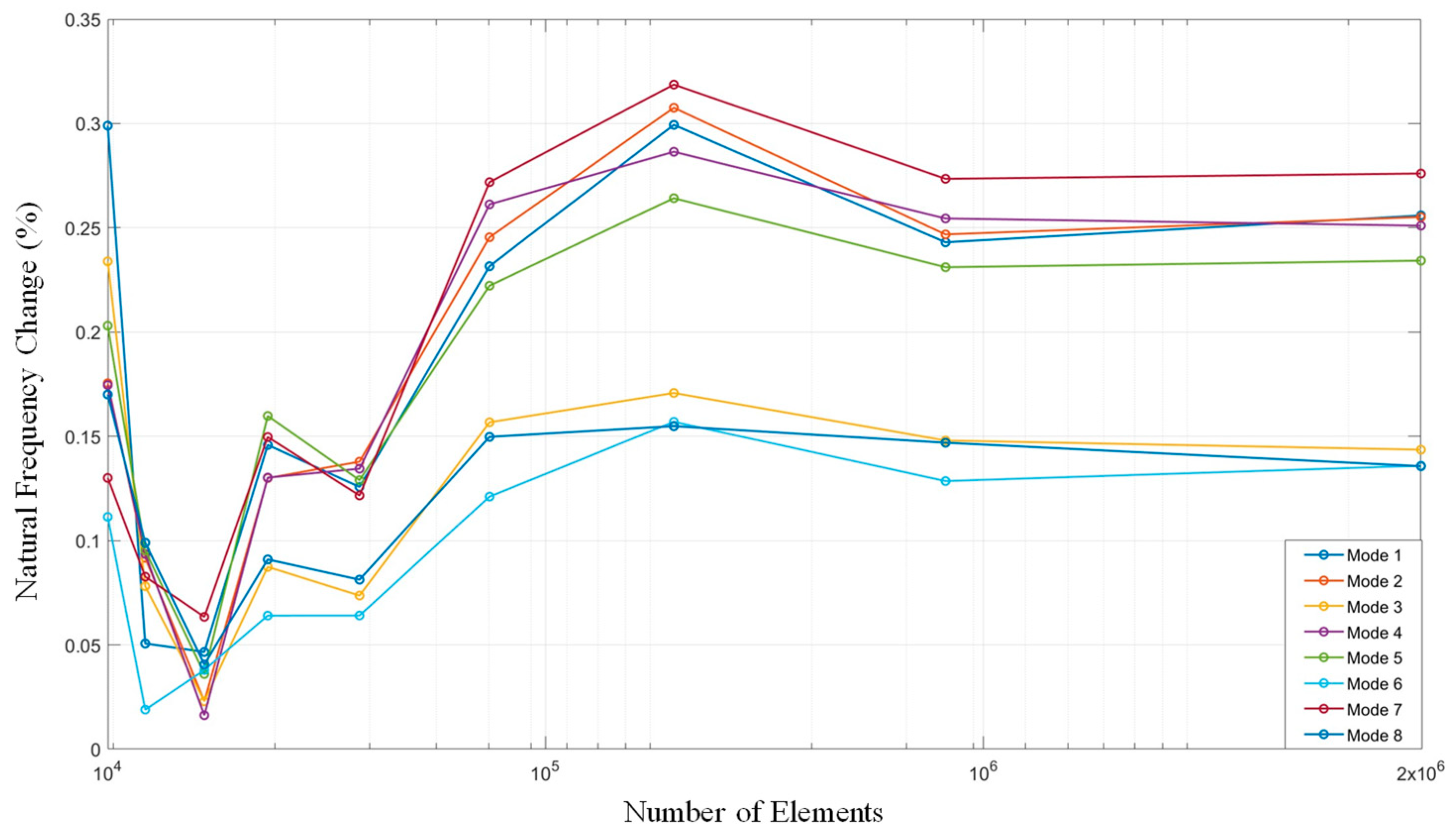
2. Computational Modal Analysis of Camshaft

The modal analysis, comprising both experimental and numerical approaches, is conducted as a cornerstone of this study to achieve precise material properties of the camshaft. This analysis provides crucial information on the essential modal parameters of the camshaft, i.e., natural frequencies and mode shapes. In this study, first, finite element method (FEM)-based computational numerical modal analysis is utilized. Next, experimental modal analysis (EMA) is performed to validate the FEM model. Hence, a comprehensive understanding of the dynamic behavior of the camshaft is obtained. In this study, solid models are developed in Autodesk Inventor platform, and FEM-based computational analyses are performed in Ansys. In the FEM model, the material properties, such as density ($\rho$), Young’s modulus ($E$), and Poisson’s ratio ($\nu$), of the camshaft are initially selected as $\rho =7200 \mathrm{k}\mathrm{g}/{\mathrm{m}}^3$, $E=110 \mathrm{G}\mathrm{P}\mathrm{a}$, and $\nu =0.29$, respectively.

In order to enhance the accuracy of the FEM model, first, a mesh refinement process is applied via mesh convergence analysis. Mesh convergence analysis is an essential step that evaluates the sensitivity of the computational model results to mesh density. Hence, it ensures the accuracy and reliability of the FEM results, i.e., accurate mesh generation and mesh density values are critical in determining the stability of the solution [48]. In this study, the mesh size is systematically decreased from 10 mm to 1 mm, where the mesh sizes of 10 mm and 1 mm correspond to $8320$ and $\mathrm{2,726,855}$ number of elements, respectively. Natural frequencies of the camshaft at the frequency range of interest, which is adopted as $0–8 \mathrm{k}\mathrm{H}\mathrm{z}$ due to constraints of the experimental setup in EMA, are calculated for each mesh size; the percental change in natural frequencies with respect to number of elements, which is inversely related to the mesh size, are depicted in Figure 1.

As observed in Figure 1, the values of the natural frequencies stabilize for the mesh size of $2 \mathrm{m}\mathrm{m}$ and below, i.e., the change in natural frequencies is minimal as the mesh size is reduced from $2 \mathrm{m}\mathrm{m}$. Hence, the mesh size in this study is selected as $2 \mathrm{m}\mathrm{m}$, which corresponds to a total number of $355$,$065$ elements, in order to reduce the computational cost. Furthermore, the average skewness value of the mesh structure is found to be below $0.5$ for $95\%$ of the elements, which suggests a high mesh quality over the entire structure. Consequently, the modal analysis is performed based on a mesh size of $2 \mathrm{m}\mathrm{m}$; the computationally calculated natural frequencies ($f_{i,FEM}$) are listed in the next section in comparison with those predicted experimentally.

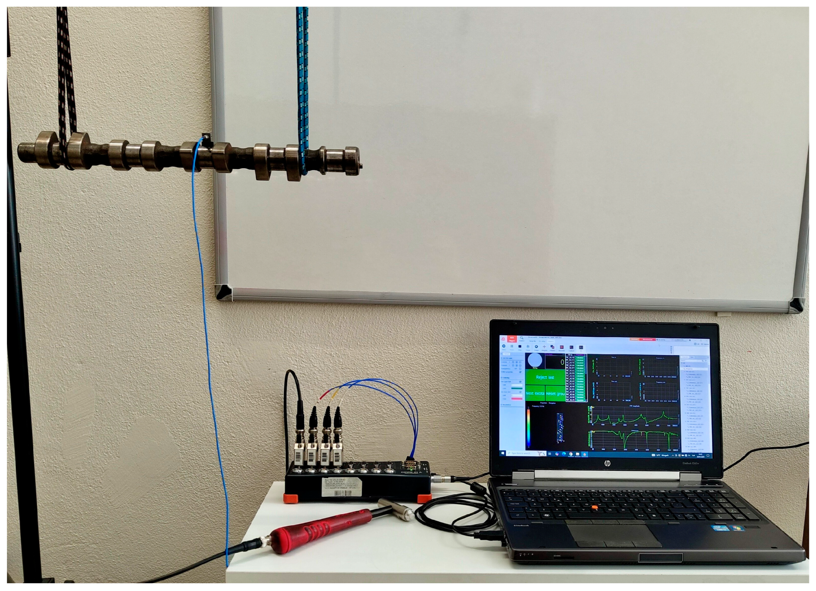
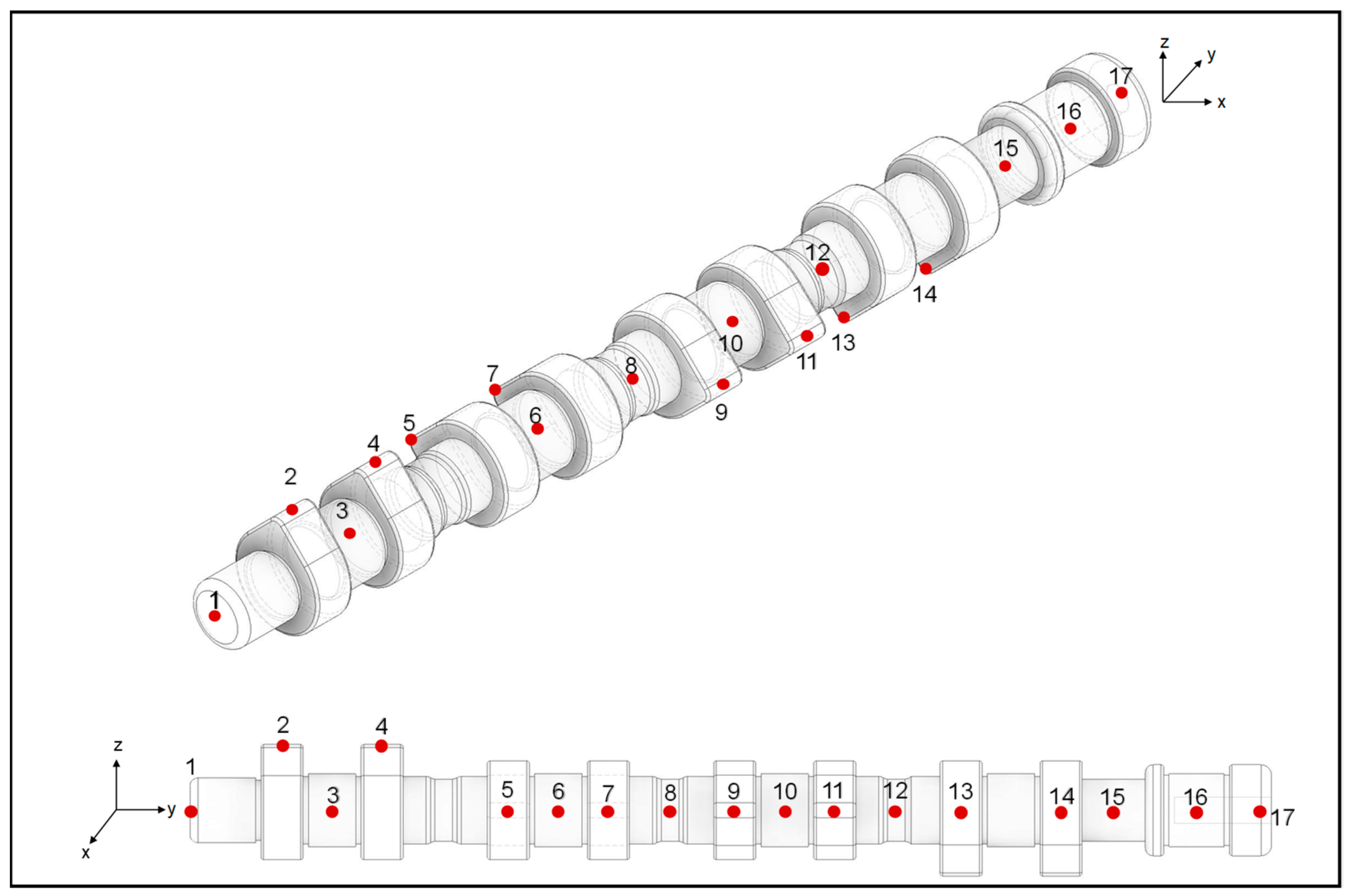
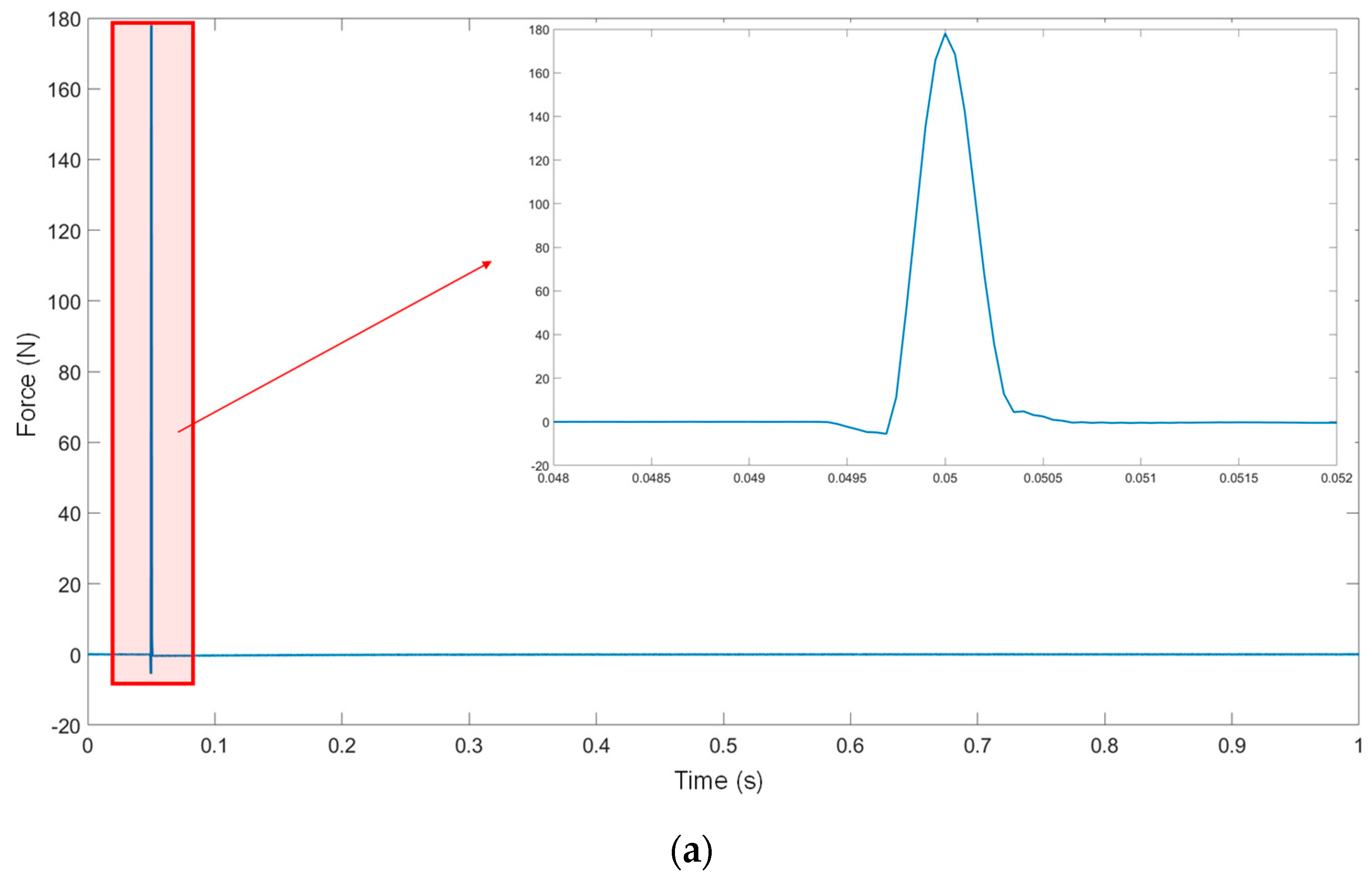
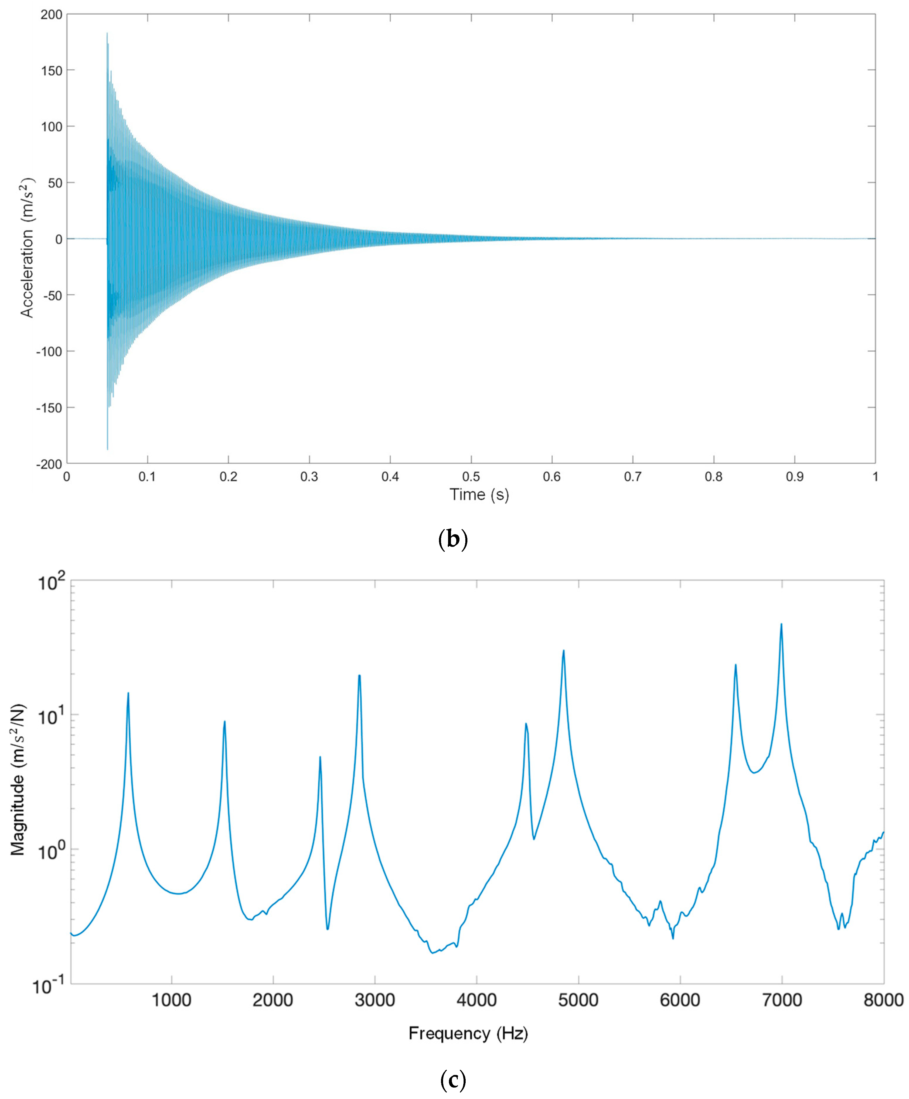
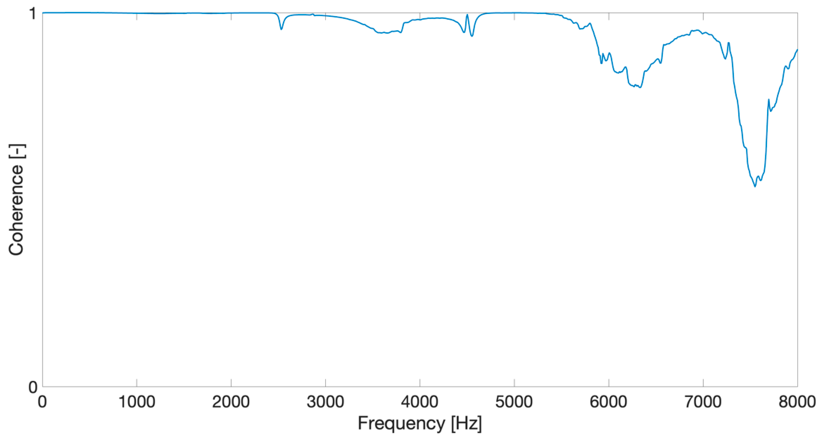
3. Experimental Modal Analysis of Camshaft

Experimental modal analysis (EMA) is performed to determine the natural frequencies and corresponding mode shapes of the camshaft, providing essential data for material property identification and numerical validation. Experimental modal analysis is a widely used technique that enables the study of a structure’s vibrational behavior under controlled conditions. In this study, the EMA technique is carefully applied to ensure high accuracy and repeatability.

In this study, the existing camshaft is tested under free–free boundary conditions to ensure that its dynamic response was not influenced by external constraints. Tests are performed with DEWE-43A Data Acquisition System and the corresponding DewesoftX (2025.1) software. Hence, the camshaft is suspended using thin, flexible ropes, which allow it to move freely in all directions. The suspension setup minimizes unwanted damping and ensures accurate representation of the camshaft’s natural vibrational behavior under free–free boundary conditions. The experimental setup for the modal analysis is illustrated in Figure 2.

The roving hammer technique is utilized during the modal tests. A modal hammer equipped with a medium tip and vinyl cover is used during excitation, and vibratory responses are measured with a triaxial accelerometer. The brand of the modal hammer used is Endevco 2302-10, which has a sensitivity of $2.25 \mathrm{m}\mathrm{V}/\mathrm{N}$. The brand of the triaxial accelerometer is PCB 356B21, which has a sensitivity of $10 \mathrm{m}\mathrm{V}/\mathrm{g}.$ During the tests, impact-type excitations are applied on 17 different points, which are distributed along the camshaft, as shown in Figure 3. The impact locations are carefully selected (eight on the camshaft profiles and nine on the shaft) to ensure that the mode shapes in the frequency range of interest are captured comprehensively. Impacts are applied in all directions that the geometry of the structure allows, i.e., three orthogonal directions at 10 points and two directions at 7 points that can be seen from the detailed list in

Table 1. List of directions of impacts applied during modal tests at all impact locations.

Impact Location	Impact Direction
1	$-x$$,+y$$,-z$
2	$-x$$,+y$$,-z$
3	$-x$$,+z$
4	$-x$$,-y$$,+z$
5	$-x$$,+y$$,+z$
6	$-x$$,-z$
7	$-x$$,-y$$,-z$
8	$-x$$,-z$
9	$-x$$,+y$$,-z$
10	$-x$$,+z$
11	$-x$$,-y$$,-z$
12	$-x$$,-z$
13	$-x$$,+y$$,+z$
14	$-x$$,-y$$,+z$
15	$-x$$,-z$
16	$-x$$,-z$
17	$-x$$,-y$$,-z$

. Furthermore, the triaxial accelerometer is positioned at point 10 in Figure 3.

Modal tests are performed with a sampling rate of $20 \mathrm{k}\mathrm{H}\mathrm{z}$, which provides a theoretical frequency range of interest of $0–10 \mathrm{k}\mathrm{H}\mathrm{z}$. However, due to the frequency range of the triaxial accelerometer, the frequency range is limited to $0–8 \mathrm{k}\mathrm{H}\mathrm{z}$, i.e., the triaxial accelerometer utilized on the setup has linear characteristics up to $8 \mathrm{k}\mathrm{H}\mathrm{z}$. Each impact event is recorded for $1 \mathrm{s}$, and recording is started with a trigger from the hammer signal. Furthermore, impacts at all excitation locations are repeated three times in order to minimize the uncorrelated noise. Hence, a total of $132$ impacts are applied during the modal test.

Data collected during modal tests (force excitation from hammer and acceleration responses from triaxial accelerometer) are recorded and transformed to the frequency domain to obtain the frequency response functions (FRFs). Transformation of time domain data to frequency domain is performed in MATLAB (R2024b), i.e., FRFs and coherence functions are calculated in MATLAB. The frequency response function represents the magnitude of the system’s response (acceleration) to input excitation (force) as a function of frequency, revealing distinct peaks corresponding to the natural frequencies of the camshaft. These peaks represent the resonance points where the camshaft exhibits significantly high vibration amplitudes. Even though a total of $132$ FRFs are calculated, only the FRF calculated based on the driving point measurement (measurement at which the excitation and response signals are collected at the same point) is depicted in Figure 4 in terms of $H_1\left(\omega \right)$ estimate, as shown below.

$$H_1\left(\omega \right)={\displaystyle \frac{S_{fx}\left(\omega \right)}{S_{ff}\left(\omega \right)}}={\displaystyle \frac{F\left(\omega \right)X^{*}\left(\omega \right)}{F\left(\omega \right)F^{*}\left(\omega \right)}}$$

(1)

where $S_{fx}\left(\omega \right)$ is the cross-spectrum of the input and output signals, $S_{ff}(\omega$) is the auto-spectrum of the input signal, $F\left(\omega \right)$ and $X\left(\omega \right)$ are the frequency spectra of the input and output signals, respectively, and * is the complex conjugate operator.

Natural frequency estimations are performed based on the Ibrahim Time Domain Method, which is a time domain approach for single input–multi-output systems [49]. This method relies on the impulse response of the system, which is essentially the case in the modal test. As is known, the displacement response of a system with $N$ degrees of freedom at the $i^{th}$ degree of freedom and at time $t=t_j$ is given as follows:

$$x_i\left(t_j\right)=\sum _{r=1}^{2N}{\Psi }_{ir}{e}^{s_r{t}_j}$$

(2)

where $s_r$ represents the eigenvalues, and ${\Psi }_{ir}$ denotes the $i^{th}$ element of the eigenvector defined as ${\Psi }_r$. In discrete time, Equation (2) can be written as follows:

$$\left[\begin{array}{cccc}{x}_1\left(t_1\right)& x_1\left(t_2\right)& \dots & x_1\left(t_L\right)\\ x_2\left(t_1\right)& x_2\left(t_2\right)& \dots & x_2\left(t_L\right)\\ ⋮& ⋮& \ddots & ⋮\\ x_q\left(t_1\right)& x_q\left(t_2\right)& \dots & x_q\left(t_L\right)\end{array}\right]=\left[\begin{array}{cccc}{\Psi }_{11}& {\Psi }_{12}& \dots & {\Psi }_{12N}\\ {\Psi }_{21}& {\Psi }_{22}& \dots & {\Psi }_{22N}\\ ⋮& ⋮& \ddots & ⋮\\ {\Psi }_{q1}& {\Psi }_{q1}& \dots & {\Psi }_{q2N}\end{array}\right]\left[\begin{array}{cccc}{e}^{s_1{t}_1}& e^{s_1{t}_2}& \dots & e^{s_1{t}_L}\\ e^{s_2{t}_1}& e^{s_2{t}_2}& \dots & e^{s_2{t}_L}\\ ⋮& ⋮& \ddots & ⋮\\ e^{s_{2N}{t}_1}& e^{s_{2N}{t}_2}& \dots & e^{s_{2N}{t}_L}\end{array}\right]$$

(3)

Note that Equation (3) can be represented in matrix form as $X=\Psi \Lambda$. Here, $q$ represents the number of signals collected from the system, and $L$ denotes the total number of discrete time steps ($t=L\Delta t$). Similarly, for $t=t_j+\Delta t$, Equation (2) takes the following form:

$$x_i\left(t_j+\Delta t\right)=\sum _{r=1}^{2N}{\Psi }_{ir}{e}^{s_r\left(t_j+\Delta t\right)}=\sum _{r=1}^{2N}\left({\Psi }_{ir}{e}^{s_r∆t}\right)e^{s_r{t}_j}$$

(4)

Defining ${\widehat{x}}_i\left(t_j\right)=x_i\left(t_j+∆t\right)$ and ${\widehat{\Psi }}_{ir}={\Psi }_{ir}{e}^{s_r∆t}$, Equation (4) becomes the following:

$${\widehat{x}}_i\left(t_j\right)=\sum _{r=1}^{2N}{\widehat{\Psi }}_{ir}{e}^{s_r{t}_j}$$

(5)

which can be written in matrix form as $\widehat{X}=\widehat{\Psi }\Lambda$. The square matrix, $A$, which is known as the system matrix, relates the matrices $\Psi$ and $\widehat{\Psi }$ through the expression $A\Psi =\widehat{\Psi }$. As a result of multiplying the expression $X=\Psi \Lambda$ by the $A$ matrix:

$$AX=A\Psi \Lambda =\widehat{\Psi }\Lambda =\widehat{X}$$

(6)

As seen in Equation (6), the system matrix $A$ relates two response states of the system at different time steps ($t_j$ and $t_j+\Delta t$), represented by the matrices $X$ and $\widehat{X}$. Since the system response matrices $X$ and $\widehat{X}$ are known, $A$ can be obtained from the solution of Equation (6). Since, the matrices $X$ and $\widehat{X}$ are not square, Equation (6) cannot be solved as $A=\widehat{X}{X}^{-1}$. Hence, two different approaches are commonly used to improve the accuracy of the modal parameter estimation [49]. These approaches are based on post multiplication of Equation (6) by the matrices $X^T$ and ${\widehat{X}}^T$ and matrix inversion. Consequently, the system matrix $A$ is obtained in two different forms as follows:

$$A=(\widehat{X}{X}^T){(X{X}^T)}^{-1}$$

(7a)

$$A=(\widehat{X}{\widehat{X}}^T){(X{\widehat{X}}^T)}^{-1}$$

(7b)

Finally, the system matrix $A$ is obtained as the arithmetic mean of Equations (7a) and (7b), as given in Equation (8).

$$A={\displaystyle \frac{1}{2}}\left[\left(\widehat{X}{X}^T\right){\left(X{X}^T\right)}^{-1}+\left(\widehat{X}{\widehat{X}}^T\right){\left(X{\widehat{X}}^T\right)}^{-1}\right]$$

(8)

From the eigenvalue solution of the system matrix $A$, natural frequencies are obtained as tabulated in

Table 2. Experimentally and computationally identified natural frequencies of camshaft.

Mode	${\mathit{f}}_{\mathit{i},\mathit{F}\mathit{E}\mathit{M}}$ [Hz]	${\mathit{f}}_{\mathit{i},\mathit{E}\mathit{M}\mathit{A}}$ [Hz]	${\mathit{ϵ}}_{\mathit{i}}$
1	488.4	576.1	17.96%
2	1293.3	1523.4	17.79%
3	2158.9	2460.9	13.99%
4	2430.2	2851.5	17.34%
5	3841.5	4482.4	16.68%
6	4193.2	4853.5	15.75%
7	5614.3	6542.9	16.54%
8	6115.0	6992.2	14.35%

together with the computationally calculated natural frequencies ($f_{i,FEM}$). Furthermore, the absolute percentage errors (${ϵ}_i$) of the $f_{i,FEM}$ are also given in Table 2, which are calculated as follows:

$${ϵ}_i=\left|{\displaystyle \frac{f_{i,FEM}-f_{i,EMA}}{f_{i,EMA}}}\right|\times 100$$

(9)

As seen from the table, a total of eight natural frequencies are identified within the frequency range of interest, and the maximum value of ${ϵ}_i$ is around 18%, which requires model updating to reduce the error, as evident from related studies in the existing literature [23,50].

In order to assess the quality of the modal test, coherence functions are also calculated at each excitation points and directions, which is a metric that reveals if the input and output signals are coherently related or not. A coherence value close to 1 indicates a strong linear relationship between the input excitation and the measured response, signifying high data quality. As seen in Figure 5, the coherence value is satisfactorily high at the frequency range of $0–6 \mathrm{k}\mathrm{H}\mathrm{z}$ for the driving point measurement (the coherence value is at the vicinity of 1), which confirms the accuracy of the conducted modal test. Beyond $6 \mathrm{k}\mathrm{H}\mathrm{z}$, the coherence value descends and deviates from 1. However, the reduction in coherence value is not significant enough to disturb the accuracy of modal parameter estimation. One reason for this deviation can be that the structure could not be excited enough at high frequencies.

4. Model Updating and Validation of Computational Model

As seen in Table 2 of the previous section, the computational (FEM) model needs to be updated for increased accuracy. Hence, the aforementioned key material parameters (density, Young’s modulus, and Poisson’s ratio) are optimized.

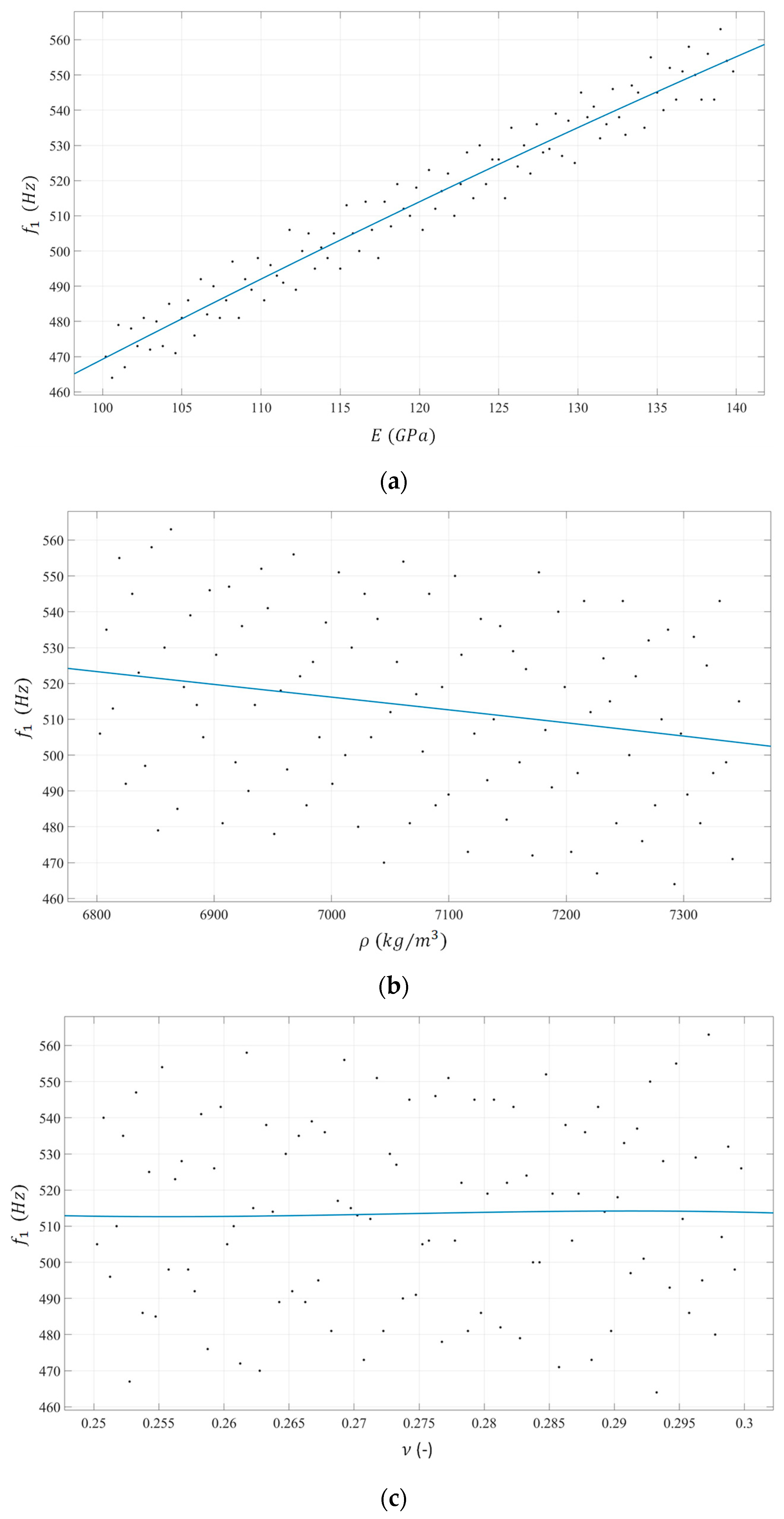
4.1. Sensitivity Analysis of Material Properties on Natural Frequencies

Sensitivity analysis is conducted as the first step of the model updating process to identify the material properties that have the most significant impact on the natural frequencies. This method focuses on the linearization of the generally nonlinear relationship between the measurable outputs and the structural model parameters that require updating [51]. Therefore, it is crucial to identify the parameters to be optimized, the tuning of which have the most effective impact on the natural frequencies, to reduce the computational cost.

The sensitivity analysis approach is based on truncated Taylor series expansion, i.e., the nonlinear terms in the series (second order and higher) are all ignored. Hence, the linear Taylor series approximation of the ith natural frequency is written as follows:

$$f_{i,FEM}\left({\rho }_j+\Delta \rho ,E_j+\Delta E,{\nu }_j+\Delta \nu \right)=f_{i,FEM}\left({\rho }_j,E_j,{\nu }_j\right)+{\left.{\displaystyle \frac{\partial f_{i,FEM}}{\partial \rho }}\right|}_{{\rho }_j,E_j,{\nu }_j}\Delta \rho +{\left.{\displaystyle \frac{\partial f_{i,FEM}}{\partial E}}\right|}_{{\rho }_j,E_j,{\nu }_j}\Delta E+{\left.{\displaystyle \frac{\partial f_{i,FEM}}{\partial \nu }}\right|}_{{\rho }_j,E_j,{\nu }_j}\Delta \mathsf{\nu }$$

(10)

where $f_{i,FEM}$ is computationally predicted ith natural frequency. Note that the linearization is carried out at a certain point of the parameter space, which is $\left[\rho ,E,\nu \right]=\left[{\rho }_j,E_j,{\nu }_j\right]$. The residual $r_i$ is defined as follows:

$$r_i=f_{i,FEM}\left(\rho +\Delta \rho ,E+\Delta E,\nu +\Delta \nu \right)-f_{i,FEM}\left(\rho ,E,\nu \right)$$

(11)

$$r_i=S_i\left\{\begin{array}{c}\Delta \rho \\ \Delta E\\ \Delta \nu \end{array}\right\}$$

(12)

where $S_i$ is expressed as follows:

$$S_i=\left[\begin{array}{ccc}{\left.{\displaystyle \frac{\partial f_{i,FEM}}{\partial \rho }}\right|}_{{\rho }_j,E_j,{\nu }_j}& {\left.{\displaystyle \frac{\partial f_{i,FEM}}{\partial E}}\right|}_{{\rho }_j,E_j,{\nu }_j}& {\left.{\displaystyle \frac{\partial f_{i,FEM}}{\partial \nu }}\right|}_{{\rho }_j,E_j,{\nu }_j}\end{array}\right]$$

(13)

Consequently, the sensitivity matrix $S$ is defined as follows based on eight natural frequencies:

$$S=\left[\begin{array}{ccc}{\left.{\displaystyle \frac{\partial f_{1,FEM}}{\partial \rho }}\right|}_{{\rho }_j,E_j,{\nu }_j}& {\left.{\displaystyle \frac{\partial f_{1,FEM}}{\partial E}}\right|}_{{\rho }_j,E_j,{\nu }_j}& {\left.{\displaystyle \frac{\partial f_{1,FEM}}{\partial \nu }}\right|}_{{\rho }_j,E_j,{\nu }_j}\\ {\left.{\displaystyle \frac{\partial f_{2,FEM}}{\partial \rho }}\right|}_{{\rho }_j,E_j,{\nu }_j}& {\left.{\displaystyle \frac{\partial f_{2,FEM}}{\partial E}}\right|}_{{\rho }_j,E_j,{\nu }_j}& {\left.{\displaystyle \frac{\partial f_{2,FEM}}{\partial \nu }}\right|}_{{\rho }_j,E_j,{\nu }_j}\\ ⋮& ⋮& ⋮\\ {\left.{\displaystyle \frac{\partial f_{8,FEM}}{\partial \rho }}\right|}_{{\rho }_j,E_j,{\nu }_j}& {\left.{\displaystyle \frac{\partial f_{8,FEM}}{\partial E}}\right|}_{{\rho }_j,E_j,{\nu }_j}& {\left.{\displaystyle \frac{\partial f_{8,FEM}}{\partial \nu }}\right|}_{{\rho }_j,E_j,{\nu }_j}\end{array}\right]$$

(14)

In this study, the sensitivity of natural frequencies to the three material properties (density, Young’s modulus, and Poisson’s ratio) are examined on a wide range of parameter space. As stated before, the initial material properties of the camshaft material are selected as $\rho =7200 \mathrm{k}\mathrm{g}/{\mathrm{m}}^3$, $E=110 \mathrm{G}\mathrm{P}\mathrm{a}$, and $\nu =0.29$. In the sensitivity analysis, these key material properties are altered in the following intervals: $6800 \mathrm{k}\mathrm{g}/{\mathrm{m}}^3\le \rho \le 7350 \mathrm{k}\mathrm{g}/{\mathrm{m}}^3$; $100 \mathrm{G}\mathrm{P}\mathrm{a}\le E\le 140 \mathrm{G}\mathrm{P}\mathrm{a}$; and $0.25\le \nu \le 0.30$. These ranges are determined based on the given initial (base) values and engineering judgment. Even though there are various types of parameter sampling techniques in sensitivity analysis, such as Latin Hypercube Sampling, Advanced Latin Hypercube Sampling, Space-Filling Latin Hypercube Sampling, Sobol Sequence, etc., the Space-Filling Latin Hypercube Sampling method is adopted in this study. This method provides a more homogeneous coverage of the input parameter space, which ensures both accuracy and diversity in the results. The space-filling characteristics of this method are particularly suitable for analyses that demand extensive sampling and comprehensive exploration of parameters [52].

For the sake of conciseness, the results of the sensitivity analysis are depicted in Figure 6 only for the first natural frequency. As observed from the figure, Young’s modulus has a significant impact on the first natural frequency, i.e., the natural frequency increases almost linearly with the increase in the Young’s modulus (Figure 6a). However, Poisson’s ratio exhibits comparatively minimal influence (Figure 6c). Furthermore, the same trend is observed for all natural frequencies at the frequency range of interest ($0–8 \mathrm{k}\mathrm{H}\mathrm{z}$).

4.2. Optimization of Material Properties

Optimization is a fundamental tool in scientific research that enables the identification of optimal solutions within defined constraints [53]. In this study, two different optimization techniques, which are Genetic Algorithm (GA) and Particle Swarm Optimization (PSO), are utilized to align the natural frequencies obtained from the computational modal analysis of the camshaft with the experimental modal analysis. Here, the chief aim is to compare the performance of these approaches (PSO and GA). Therefore, the computational cost is not a primary concern. However, the PSO approach is observed to be faster than the GA approach, which is also supported in the literature [26,50]. These methods are well suited for solving complex and nonlinear optimization problems and ensure that the developed model more accurately reflects the real-world behavior [54]. As observed in the sensitivity analysis, only two of the three material properties, namely density and Young’s modulus, are found to have a significant effect on natural frequencies. Hence, the Poisson’s ratio is kept intact in the optimization process, and the optimization is performed by tuning the density and Young’s modulus parameters of the camshaft material. Note that the optimization problem in this study is a constraint optimization problem, where the feasible set (parameter space where all constraints are satisfied) is bounded with the upper and lower boundaries of the optimization parameters (density and Young’s Modulus). Hence, the optimized parameters are expected to be the global optimum in the feasible set.

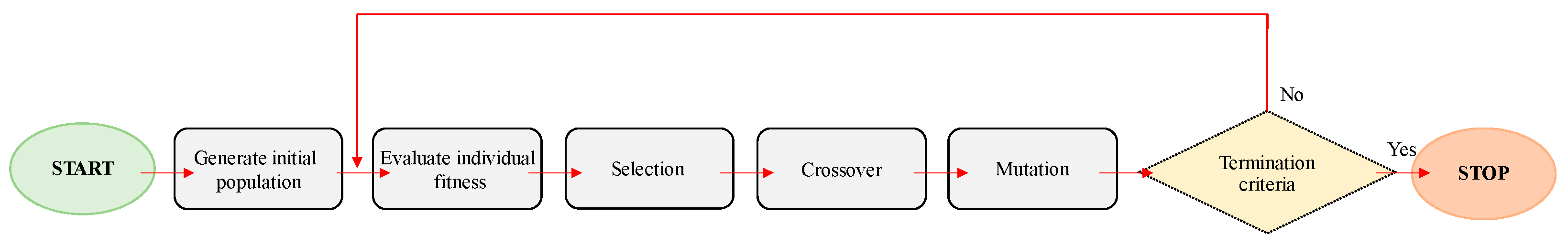
4.2.1. Genetic Algorithm

Genetic Algorithm, which was introduced by Holland [55], represents a stochastic global searching technique based on global evaluation process. The fundamental principles of evolutionary algorithms are based on the concepts of natural selection and genetic variation. In this process, the strongest individuals in a population are more likely to survive and reproduce, therefore transmitting their genetic material to the next generation [53]. Evolutionary Algorithm (EA) has been widely used in various disciplines, including modal analysis due to their robust problem-solving capabilities [56,57,58,59].

The application of GA is initiated by generating the individuals (i.e., density and Young’s modulus) in the solution space as a genetic sequence. Next, the initial population is created to comprehensively represent the solution space and new individuals are produced by the combination of randomly selected parent chromosomes with using crossover operations, therefore providing a broader exploration of the solution space. Finally, mutation is performed by randomly changing certain parts of the parent chromosomes in order to add new information to the population. This step prevents convergence at an early stage by preserving diversity and increases the local search ability of the algorithm. Depending on the convergence of the FEM-based modal analysis results to the EMA data, individuals with low objective function values are given a greater chance of being selected for the next generations. Furthermore, the objective function used in this study aims to minimize the differences between the experimental and analytical natural frequencies for all eight vibration modes. Hence, the objective function is defined in terms of the root mean square error, as given in Equation (15).

$$minimize\sqrt{{\displaystyle \frac{{\sum }_{i=1}^8{\left(f_{i,EMA}-f_{i,FEM}\right)}^2}{8}}}$$

(15)

where $f_{i,EMA}$ and $f_{i,FEM}$ are the $i^{th}$ natural frequency obtained based on modal tests and FEM-based modal analysis, respectively. The stopping criterion for the GA-based optimization process is selected as the maximum number of iterations, taken as $100$, which is found to be satisfactory based on the optimization results. The flowchart of the optimization process based on GA is depicted in Figure 7.

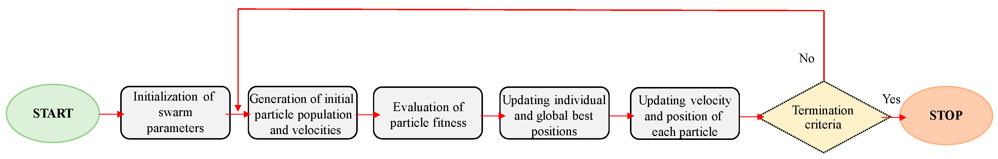
4.2.2. Particle Swarm Optimization

Particle Swarm Optimization, which was introduced by Kennedy and Eberhart [60], is inspired by food foraging, social behavior, and movement patterns of bird flocks and fish schools. Particle swarm optimization aims to optimize the balance between global and local solutions by simulating the movement of a particle swarm towards a specific target. Each particle represents a candidate solution in the solution space of the problem and updates its movement based on both its own experience and the best experience of the swarm [61,62].

In this study, the position of each particle represents a unique combination of the selected material properties (density and Young’s modulus). Velocity refers to the rate at which the particles are moving in the space, determining the particle’s position at the next moment. Hence, the moving process of particles is equivalent to the optimization of the material properties of the camshaft. During the movement of particles in the search space, particles perform two types of learning: social and cognitive learning. Each particle learns from the experiences of other particles (social learning) and from its own individual experiences (cognitive learning). As an outcome of cognitive learning, every particle records its best position, referred to as $pbest$. While engaging in social learning, particles also identify the best solution encountered within the global neighborhood, known as $gbest$, which is the best position of the swarm. During the iterations, the best position reached by each particle ($pbest$) and the best overall position reached by the swarm ($gbest$) are recorded. This information is used to update the particle velocities and hence their positions. This process is mathematically explained with the following equations:

$$v_i^{t+1}=w\times v_i^t+c_1\times r_1\left(x_{pbest,i}^t-x_i^t\right)+c_2\times r_2\left(x_{gbest,i}^t-x_i^t\right)$$

(16a)

$$x_i^{t+1}=x_i^t+v_i^{t+1}$$

(16b)

where $v_i^t$ and $v_i^{t+1}$ are the current and updated velocities of the ith particle, respectively. Similarly, $x_i^t$ refers to the current and $x_i^{t+1}$ represents the updated positions of the ith particle. Furthermore, the $pbest$ of the ith particle and the $gbest$ of the swarm are represented with $x_{pbest,i}^t$ and $x_{gbest}^t$, respectively. The parameters $c_1$ and $c_2$ are acceleration coefficients, $w$ refers to the inertia factor, and $r_1$ and $r_2$ indicate the random numbers drawn from the interval of (0,1) using uniform distribution. As in GA-based optimization, the same objective function (Equation (15)) is used in PSO. Consequently, the fitness of each particle is evaluated based on the defined objective function, and particle velocities and positions are updated. Finally, the process completes when the stopping criterion is met, yielding the optimal values for Young’s Modulus and density. Similarly to the GA-based optimization process, the stopping criterion is again selected as the maximum number of iterations. The flowchart of the PSO-based optimization process is given below in Figure 8.

4.2.3. Results of Optimization Process

Based on the application of the GA and PSO techniques, the optimum values of the material properties are calculated and listed in

Table 3. The values of the material properties based on the optimization process.

Material Property	Initial Value	Genetic Algorithm		Particle Swarm Optimization
		Updated Value	Relative Change	Updated Value	Relative Change
$\rho$ $[\mathrm{k}\mathrm{g}/{\mathrm{m}}^3$]	$7200$	$6833.98$	$5.08\%$	$6826.94$	$5.18\%$
$E$ $[\mathrm{G}\mathrm{P}\mathrm{a}$]	$110$	$140.00$	$27.27\%$	$139.88$	$27.17\%$

. As seen from the table, both optimization approaches provide similar results for both material properties. The optimum density value is found to be approximately $6830 \mathrm{k}\mathrm{g}/{\mathrm{m}}^3$, which implies a relative change (reduction) of $5.10\%$. Furthermore, the optimum value of the Young’s modulus is calculated as $140 \mathrm{G}\mathrm{P}\mathrm{a}$, which is a relative change (increase) of $27.17\%$.

Finally, the computational model is updated with the optimized parameters, and the calculated natural frequencies with the optimized parameters are given in

Table 4. Natural frequencies of updated camshaft model.

$\mathit{i}$	${\mathit{f}}_{\mathit{i},\mathit{E}\mathit{M}\mathit{A}}$ $\mathbf{[}\mathbf{H}\mathbf{z}$]	Genetic Algorithm		Particle Swarm Optimization
		${\mathit{f}}_{\mathit{i},\mathit{F}\mathit{E}\mathit{M},\mathit{G}\mathit{A}}$ $\mathbf{[}\mathbf{H}\mathbf{z}$]	${\mathit{ϵ}}_{\mathit{i},\mathit{G}\mathit{A}}$ $\mathbf{[}\mathbf{\%}$]	${\mathit{f}}_{\mathit{i},\mathit{F}\mathit{E}\mathit{M},\mathit{P}\mathit{S}\mathit{O}}$ $\mathbf{[}\mathbf{H}\mathbf{z}$]	${\mathit{ϵ}}_{\mathit{i},\mathit{P}\mathit{S}\mathit{O}}$ $\mathbf{[}\mathbf{\%}$]
$1$	$576.1$	$566.0$	$1.7$	$566.1$	$1.7$
$2$	$1523.4$	$1498.8$	$1.6$	$1498.9$	$1.6$
$3$	$2460.9$	$2490.3$	$1.2$	$2490.5$	$1.2$
$4$	$2851.5$	$2816.0$	$1.2$	$2816.3$	$1.2$
$5$	$4482.4$	$4450.6$	$0.7$	$4451.0$	$0.7$
$6$	$4853.5$	$4858.3$	$0.1$	$4858.8$	$0.1$
$7$	$6542.9$	$6503.6$	$0.6$	$6504.3$	$0.6$
$8$	$6992.2$	$7053.9$	$0.9$	$7054.6$	$0.9$

. As observed from the table, the maximum relative error in the updated model is reduced below $2\%$, which is around $18\%$ based on the initial values of the parameters. Hence, it is concluded that the optimization process successfully determines the desired material properties.

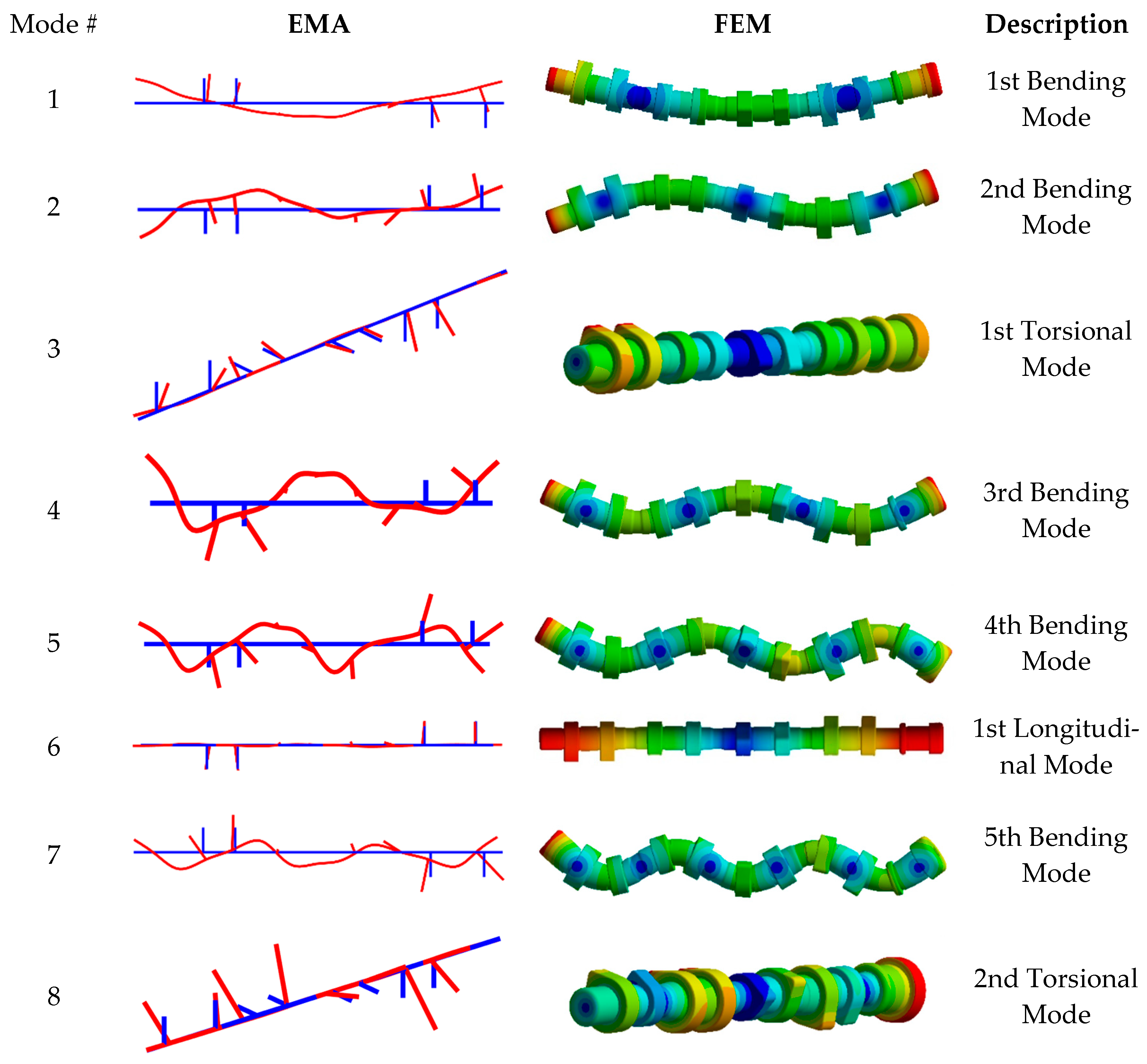
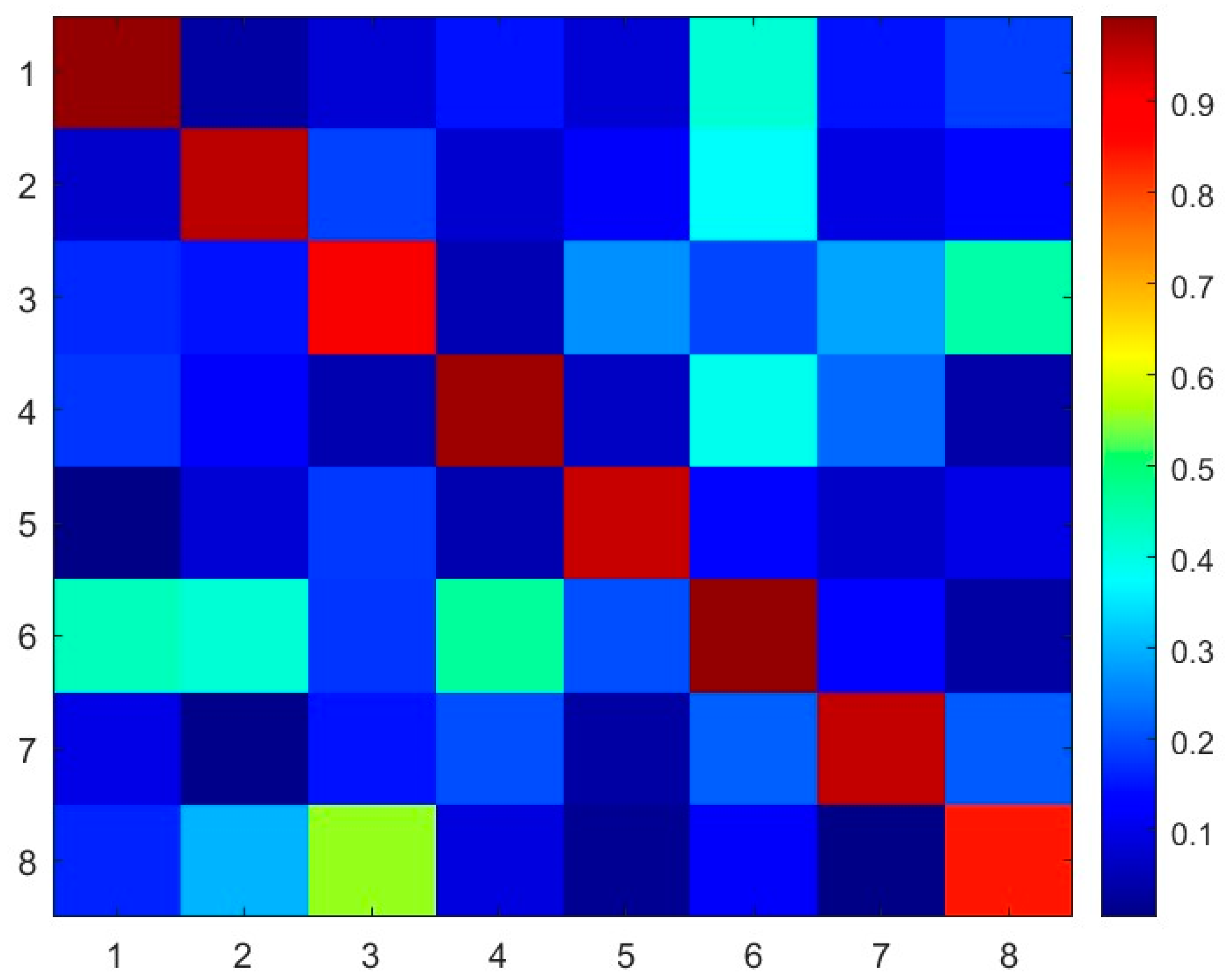
4.3. Comparison of Mode Shapes via Modal Assurance Criteria

As explained in the optimization section of this study, the computational model of the camshaft is successfully validated with the experimental data based on the natural frequencies at the frequency range of interest. However, it is crucial to assess the order of the mode shapes for in-depth validation. Hence, first, the mode shapes of the EMA- and FEM-based modal analysis are obtained and depicted in Figure 9. The process of mode shape estimation of EMA data is performed with a homemade MATLAB script prepared in this study. As seen from Figure 9, the mode shapes estimated computationally successfully resemble the experimental counterparts, and the frequency range of interest is dominated by bending, torsional, and longitudinal modes.

Even though the resemblance between the experimental and computational mode shapes are visually seen in Figure 9, they are also compared mathematically via Modal Assurance Criterion (MAC).

Modal Assurance Criterion, which is a commonly used tool for the quantitative comparison of modal vectors, compares the similarity of eigenvectors based on Equation (17). Hence, MAC is used as an indicator in this study to measure the consistency between experimentally and analytically obtained mode shapes, which is a common approach in the existing literature [37,38,39,40]. The value of MAC is bounded between 0 and 1, where 1 indicates that the compared mode shapes are identical and 0 indicates no similarity. In general, an MAC value greater than 0.9 indicates that modal shapes are completely consistent [31,63]. The calculation of the MAC value is given in Equation (17). The symbol $\phi$ in Equation (17) corresponds to mode shapes and the subscripts EMA and FEM denote the approach that the mode shapes are calculated. Hence, ${\phi }_{EMA}$ is the mode shapes estimated via experimental data (modal test) and ${\phi }_{FEM}$ is the mode shapes calculated computationally through the FEM approach. Furthermore, subscripts $r$ and $q$ point out the rth and qth modes of the EMA and FEM approaches, respectively, and the superscript $T$ is the transpose operator.

$$MAC\left(r,q\right)={\displaystyle \frac{{\left|{\left\{{\phi }_{EMA}\right\}}_r^T{\left\{{\phi }_{FEM}\right\}}_q\right|}^2}{\left({\left\{{\phi }_{EMA}\right\}}_r^T{\left\{{\phi }_{EMA}\right\}}_r\right)\left({\left\{{\phi }_{FEM}\right\}}_q^T{\left\{{\phi }_{FEM}\right\}}_q\right)}}$$

(17)

The comparison of mode shapes based on MAC values are shown in Figure 10. As seen, the MAC values on the main diagonal of the MAC table are at the vicinity of 0.9, which indicates a strong correlation between the two eigenvectors.

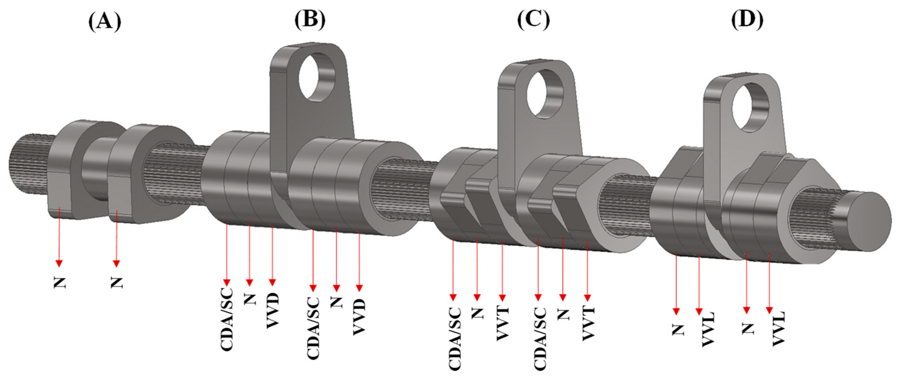
5. Modified Camshaft Mechanism with Multiple Operating Modes

The camshaft mechanism developed in this study aims to provide a functionally flexible system that can adapt to different load and speed conditions of the engine by integrating multiple valve control strategies. While existing systems in the literature are designed to implement only a limited combination of such strategies, the configuration presented in this study enables incremental application of multiple methods such as Variable Valve Timing (VVT), Variable Valve Lift (VVL), Variable Valve Duration (VVD), Cylinder Deactivation (CDA), and Skip Cycle (SC) within a single camshaft design.

This multi-mode configuration allows different operating modes to be applied individually to each cylinder, thus optimizing the fuel consumption and efficiency of the engine based on driving conditions. In particular, the skip cycle mode enables a reduction fuel consumption of up to approximately 25% at low engine speeds [64].

The proposed mechanism is based on a modular cam profile system that enables multiple operating modes. As shown in Figure 11, the proposed mechanism consists of optimized four modules (A, B, C, and D). Each module is designed with different cam profiles corresponding to a specific valve control strategy. These modules are positioned on a spline shaft, i.e., cam profile groups in modules B, C, and D can slide axially along the shaft. The sliding motion of these cam profile groups are applied through different forks which are driven by ball screw mechanisms. Hence, it is crucial to minimize any vibration of the shaft in the longitudinal and radial axes to guarantee the proper operation of the mechanism.

As opposed to the original design, the proposed mechanism supports five distinct operating modes and the combinations. These modes include the normal mode (N), which utilizes a standard cam profile representing conventional operation; the Variable Valve Duration (VVD) mode, which alters the time duration that the valve remains open; the Variable Valve Timing (VVT) mode, which adjusts the timing of valve opening and closing events; the Variable Valve Lift (VVL) mode, which modifies the valve lift; and the Cylinder Deactivation/Skip Cycle (CDA/SC) mode, which uses a flat base circle profile to prevent valve opening entirely. Even though CDA and SC modes utilize the same cam profile, they differ significantly in operation. Cylinder Deactivation (CDA) completely disables selected cylinders for extended operation periods. Skip Cycle (SC) selectively disables valve actuation only for specific engine cycles [65].

As depicted in Figure 11 and

Table 5. List of operation modes on different modules.

Module	Profile 1	Profile 2	Profile 3
$\mathrm{A}$	$N$	$-$	$-$
$\mathrm{B}$	$CDA/SC$	$N$	$VVD$
$\mathrm{C}$	$CDA/SC$	$N$	$VVD$
$\mathrm{D}$	$N$	$VVL$	$-$

, the mechanism relies on cascading a group of different cam profiles and sliding them over the camshaft in order to activate different modes of operations. For example, no modifications are applied to module A, i.e., module A operates in normal mode (N) since it has a single profile, which is the same as the original design in Figure 3. In module B, three different cam profiles are used which can active the modes of CDA/SC, N, and VVD. In module C, again, three different cam profiles are utilized, and these profiles are used to activate the modes of CDA/SC, N, and VVT. Finally, only two cam profiles are selected for module D, which can initiate the modes of N and VVL.

Note that all cam profiles should be designed for the activation of the corresponding mode of operation. However, the cam profile for the CDA/SC mode is simply the base circle, which does not excite valves. Due to the existence of two valves in the engine, the cam profiles are implemented to the modules in two sets. Furthermore, transition between modes is provided by the axial movement of the modules. As evident from the available literature [66,67,68], this configuration aims to optimize engine efficiency by selecting the appropriate mode based on driving conditions.

It is important to highlight that the variable number of cam profiles designed for each cylinder in the modules leads to structural asymmetry in the camshaft. This asymmetric distribution requires careful dynamic analysis, especially in terms of vibration characteristics, and it is critical for the reliability and operational integrity of the mechanism. Furthermore, under asymmetrical valve system loading conditions, modal analysis provides critical information about the proper selection of non-uniform camshaft journal bearing locations and dimensions.

In addition to structural and operational asymmetry, another critical aspect arises from the axial motion of the cams on the shaft of the mechanism used for selectable mode switching by the individually driven cams. As the mechanism relies on axial motion for different mode switching, its dynamic behavior in the longitudinal direction (y axis in Figure 3) must be carefully evaluated. In particular, vibrations at high engine speeds could cause unintended module shifts or valve timings and displacement inaccuracies during transitions. Hence, a detailed modal analysis, i.e., investigation of modal parameters such as natural frequencies and mode shapes, is conducted during the design process. Considering these critical aspects, a validated dynamic model is essential not only for understanding vibration characteristics but also for ensuring reliable mechanism operation beside the combustion process under realistic operating conditions.

The optimization process yields a validated model by aligning the original camshaft’s modal analysis results with experimental data. Hence, the validated model serves as a basis for the modified camshaft design in order to investigate its dynamic characteristics. Subsequently, the natural frequencies and mode shapes of the modified mechanism are obtained computationally based on the FEM model, which is developed as an extension of the validated model. The natural frequencies of the modified design are listed in

Table 6. Natural frequencies of modified camshaft with multiple operating modes.

$\mathit{i}$	${\mathit{f}}_{\mathit{i}}$ $\left[\mathbf{H}\mathbf{z}\right]$	$\mathit{i}$	${\mathit{f}}_{\mathit{i}}$ $\left[\mathbf{H}\mathbf{z}\right]$
$1$	$583.8$	$6$	$4718.7$
$2$	$1582$	$7$	$5116.6$
$3$	$2086.7$	$8$	$5471$
$4$	$2804.9$	$9$	$5883.3$
$5$	$3787.8$	$10$	$7136.2$

, and the corresponding mode shapes are depicted in Figure 12. First, it should be mentioned that a total number of 10 natural frequencies are calculated in the frequency range of $0–8 \mathrm{k}\mathrm{H}\mathrm{z}$, which is two more than the original design. Furthermore, the value of the first natural frequency, which is $583.8 \mathrm{H}\mathrm{z}$, is found to be intact (around $2\%$ higher) when compared to the original design. This frequency is still well above the maximum operating speed of the engine. Hence, it is not expected to observe resonance phenomenon due to engine speed excitation. In terms of the mode shapes, the modified design exhibits a mode (mode #6) which is a combination of the shaft and the attached mechanisms. Furthermore, three modes (mode #7, 8, 9) are observed to be purely related to fork motion. Brief explanations of these mode shapes are provided in Figure 12. It is observed that the first torsional mode frequency of the modified camshaft is reduced; the deviations of the third and fourth bending mode frequencies of the modified camshaft are minimal; and the first longitudinal mode frequency is shifted to higher frequencies (beyond the frequency range of interest). Particularly, the shift in longitudinal mode frequency is of importance, since it may disturb the shifting operation of cam profile groups.

6. Conclusions

This study investigates the modal performance of an existing camshaft design computationally, utilizes experimental modal analysis for validating the existing computational model, and develops a novel camshaft mechanism based on the validated model that integrates multiple engine control strategies into a single structure.

A mesh convergence analysis determines that an element size of $2 \mathrm{m}\mathrm{m}$ provides a balance between accuracy and computational cost. A validated FEM model is obtained by aligning computational results with experimental modal analysis through sensitivity-based model updating and optimization using GA and PSO algorithms, leading to a maximum relative frequency error from an initial 18% to below 2%. The MAC analysis further confirms consistency between the experimental and computational mode shapes, with the main diagonal elements of the MAC matrix reaching values around 0.9. As a result, a validated computational model of the existing camshaft is obtained.

Finally, the validated model is used as a basis for a modified camshaft system design, which integrates multiple modes of operations, i.e., different VVA, Cylinder Deactivation, and Skip Cycle strategies are enabled on the internal combustion engine with this mechanism. The new design is investigated from the perspective of modal characteristics, and its natural frequencies and mode shapes are obtained. Even though the mode shapes of the modified mechanism resemble the original design, some of the modes are shifted beyond the frequency range of interest. In particular, the longitudinal mode frequency is now shifted to a higher band. This suggests that the mechanism’s dynamic behavior will not interfere with its functional operation, especially during longitudinal displacement. In this context, modal analysis provides both a verification method and a useful tool to evaluate possible resonance risks in the proposed system. Hence, it is guaranteed that the operation of the mechanism is not disturbed by the elastic modes, while the vibration performance of the proposed design remains compatible with the original system, confirming that additional valve functionalities can be integrated without compromising its dynamic behavior. In conclusion, the modified mechanism has advantages in terms of fuel economy and efficiency while exhibiting similar modal characteristics [64,65,66,67]. This integrated design approach, which combines multiple engine control strategies within a single camshaft architecture, constitutes one of the key technical contributions of this study.

In summary, the major outcomes of the study are as follows: (1) The $2 \mathrm{m}\mathrm{m}$ mesh size is found to be the optimal dimension for both computational cost and natural frequency prediction accuracy. (2) It is observed that the Poisson’s ratio does not significantly affect the natural frequencies. (3) Even though both optimization algorithms (PSO and GA) give similar results, it is seen that the PSO approach is superior from the perspective of computational cost. (4) Modal studies performed reveal that both designs do not have a resonance problem which could be triggered by engine operation. (5) It is shown for the new design that the longitudinal vibration mode is moved to a higher frequency band, which is critical for the operation of new design, ensuring safe implementation.

In this study, the new design is not manufactured. Hence, the validation of the computational model is performed on the existing design, which is also physically available. However, it is expected to achieve a reduction in fuel consumption with this proposed mechanism based on prior studies [64,65]. As future work, first, it is aimed to develop a one-dimensional engine model to assess the fuel consumption performance of the proposed design. Furthermore, the proposed optimal design can be manufactured and installed on the engine for testing.

References

1. Douglas, K.J.; Milovanovic, N.; Turner, J.; Blundell, D. Fuel Economy Improvement Using Combined CAI and Cylinder Deactivation (CDA)—An Initial Study; SAE Technical Paper; SAE International: Warrendale, PA, USA, 2005; p. 2005-01-0110. [Google Scholar] [CrossRef]
2. Rebbert, M.; Kreusen, G.; Lauer, S. A New Cylinder Deactivation by FEV and Mahle; SAE Technical Paper; SAE International: Warrendale, PA, USA, 2008; p. 2008-01-1354. [Google Scholar] [CrossRef]
3. Zhao, J.; Xi, Q.; Wang, S.; Wang, S. Improving the Partial-Load Fuel Economy of 4-Cylinder SI Engines by Combining Variable Valve Timing and Cylinder-Deactivation through Double Intake Manifolds. Appl. Therm. Eng. 2018, 141, 245–256. [Google Scholar] [CrossRef]
4. Flierl, R.; Lauer, F.; Breuer, M.; Hannibal, W. Cylinder Deactivation with Mechanically Fully Variable Valve Train. SAE Int. J. Engines 2012, 5, 207–215. [Google Scholar] [CrossRef]
5. Falkowski, A.; McElwee, M.; Bonne, M. Design and Development of the DaimlerChrysler 5.7L HEMI® Engine Multi-Displacement Cylinder Deactivation System; SAE Technical Paper; SAE International: Warrendale, PA, USA, 2004; p. 2004-01-2106. [Google Scholar] [CrossRef]
6. Hatano, K.; Iida, K.; Higashi, H.; Murata, S. Development of a New Multi-Mode Variable Valve Timing Engine. SAE Trans. 1993, 102, 930878. [Google Scholar] [CrossRef]
7. Hosaka, T.; Hamazaki, M. Development of the Variable Valve Timing and Lift (VTEC) Engine for the Honda NSX; SAE Technical Paper; SAE International: Warrendale, PA, USA, 1991; p. 910008. [Google Scholar] [CrossRef]
8. Huber, R.; Klumpp, P.; Ulbrich, H. Dynamic Analysis of the Audi Valvelift System. SAE Int. J. Engines 2010, 3, 839–849. [Google Scholar] [CrossRef]
9. Millo, F.; Mirzaeian, M.; Luisi, S.; Doria, V.; Stroppiana, A. Engine Displacement Modularity for Enhancing Automotive s.i. Engines Efficiency at Part Load. Fuel 2016, 180, 645–652. [Google Scholar] [CrossRef]
10. Fukui, T.; Nakagami, T.; Endo, H.; Katsumoto, T.; Danno, Y. Mitsubishi Orion-MD—A New Variable Displacement. SAE Trans. 1983, 92, 362–370. [Google Scholar]
11. Maas, G.; Neukirchner, H.; Dingel, O.; Predelli, O. Potential of an Innovative, Fully Variable Valvetrain; SAE Technical Paper; SAE International: Warrendale, PA, USA, 2004; p. 2004-01-1393. [Google Scholar] [CrossRef]
12. Brüstle, C.; Schwarzenthal, D. VarioCam Plus—A Highlight of the Porsche 911 Turbo Engine; SAE Technical Paper; SAE International: Warrendale, PA, USA, 2001; p. 2001-01-0245. [Google Scholar] [CrossRef]
13. Azarniya, O.; Forooghi, A. Integrated Analysis of Free Vibrations in Hyperelastic Beams: Numerical Methods, Experimental Validation, and Neural Network Predictions. Multiscale Multidiscip. Model. Exp. Des. 2025, 8, 85. [Google Scholar] [CrossRef]
14. Borgonovo, E.; Plischke, E. Sensitivity Analysis: A Review of Recent Advances. Eur. J. Oper. Res. 2016, 248, 869–887. [Google Scholar] [CrossRef]
15. Bakir, P.G.; Reynders, E.; De Roeck, G. Sensitivity-Based Finite Element Model Updating Using Constrained Optimization with a Trust Region Algorithm. J. Sound Vib. 2007, 305, 211–225. [Google Scholar] [CrossRef]
16. Bianconi, F.; Salachoris, G.P.; Clementi, F.; Lenci, S. A Genetic Algorithm Procedure for the Automatic Updating of FEM Based on Ambient Vibration Tests. Sensors 2020, 20, 3315. [Google Scholar] [CrossRef]
17. Marwala, T. Finite-Element-Model Updating Using Computional Intelligence Techniques; Springer: London, UK, 2010. [Google Scholar] [CrossRef]
18. Villa, M.; Ferreira, B.; Cruz, N. Genetic Algorithm to Solve Optimal Sensor Placement for Underwater Vehicle Localization with Range Dependent Noises. Sensors 2022, 22, 7205. [Google Scholar] [CrossRef] [PubMed]
19. Boonlong, K. Vibration-Based Damage Detection in Beams by Cooperative Coevolutionary Genetic Algorithm. Adv. Mech. Eng. 2014, 6, 624949. [Google Scholar] [CrossRef]
20. Tu, Z.; Lu, Y. FE Model Updating Using Artificial Boundary Conditions with Genetic Algorithms. Comput. Struct. 2008, 86, 714–727. [Google Scholar] [CrossRef]
21. Girardi, M.; Padovani, C.; Pellegrini, D.; Robol, L. A Finite Element Model Updating Method Based on Global Optimization. Mech. Syst. Signal Process. 2021, 152, 107372. [Google Scholar] [CrossRef]
22. Park, G.; Hong, K.-N.; Yoon, H. Vision-Based Structural FE Model Updating Using Genetic Algorithm. Appl. Sci. 2021, 11, 1622. [Google Scholar] [CrossRef]
23. Liu, T.; Zhang, Q.; Zordan, T.; Briseghella, B. Finite Element Model Updating of Canonica Bridge Using Experimental Modal Data and Genetic Algorithm. Struct. Eng. Int. 2016, 26, 27–36. [Google Scholar] [CrossRef]
24. Alkayem, N.F.; Cao, M.; Zhang, Y.; Bayat, M.; Su, Z. Structural Damage Detection Using Finite Element Model Updating with Evolutionary Algorithms: A Survey. Neural Comput. Appl. 2018, 30, 389–411. [Google Scholar] [CrossRef]
25. Mojtahedi, A.; Baybordi, S.; Fathi, A.; Yaghubzadeh, A. A Hybrid Particle Swarm Optimization and Genetic Algorithm for Model Updating of A Pier-Type Structure Using Experimental Modal Analysis. China Ocean. Eng. 2020, 34, 697–707. [Google Scholar] [CrossRef]
26. Tran-Ngoc, H.; Khatir, S.; De Roeck, G.; Bui-Tien, T.; Nguyen-Ngoc, L.; Abdel Wahab, M. Model Updating for Nam O Bridge Using Particle Swarm Optimization Algorithm and Genetic Algorithm. Sensors 2018, 18, 4131. [Google Scholar] [CrossRef]
27. Wang, S.; Xiang, B.; Wang, W.; Lian, P.; Zhao, Y.; Cui, H.; Lin, S.; Zhou, J. Finite Element Model Updating Method for Radio Telescope Antenna Based on Parameter Optimization with Surrogate Model. Appl. Sci. 2024, 14, 5620. [Google Scholar] [CrossRef]
28. Shabbir, F.; Omenzetter, P. Model Updating Using Genetic Algorithms with Sequential Niche Technique. Eng. Struct. 2016, 120, 166–182. [Google Scholar] [CrossRef]
29. Levin, R.I.; Lieven, N.A.J. Dynamic Finite Element Model Updating Using Simulated Annealing and Genetic Algorithms. Mech. Syst. Signal Process. 1998, 12, 91–120. [Google Scholar] [CrossRef]
30. Allemang, R.J. The Modal Assurance Criterion—Twenty Years of Use and Abuse. Sound Vib. 2003, 37, 14–23. [Google Scholar]
31. Pastor, M.; Binda, M.; Harčarik, T. Modal Assurance Criterion. Procedia Eng. 2012, 48, 543–548. [Google Scholar] [CrossRef]
32. Jin, S.-S.; Cho, S.; Jung, H.-J.; Lee, J.-J.; Yun, C.-B. A New Multi-Objective Approach to Finite Element Model Updating. J. Sound Vib. 2014, 333, 2323–2338. [Google Scholar] [CrossRef]
33. Zárate, B.A.; Caicedo, J.M. Finite Element Model Updating: Multiple Alternatives. Eng. Struct. 2008, 30, 3724–3730. [Google Scholar] [CrossRef]
34. Zhou, X.; Kim, C.-W.; Zhang, F.-L.; Chang, K.-C. Vibration-Based Bayesian Model Updating of an Actual Steel Truss Bridge Subjected to Incremental Damage. Eng. Struct. 2022, 260, 114226. [Google Scholar] [CrossRef]
35. Simoen, E.; De Roeck, G.; Lombaert, G. Dealing with Uncertainty in Model Updating for Damage Assessment: A Review. Mech. Syst. Signal Process. 2015, 56–57, 123–149. [Google Scholar] [CrossRef]
36. Arora, V. Comparative Study of Finite Element Model Updating Methods. J. Vib. Control. 2011, 17, 2023–2039. [Google Scholar] [CrossRef]
37. Jung, D.-S.; Kim, C.-Y. Finite Element Model Updating on Small-Scale Bridge Model Using the Hybrid Genetic Algorithm. Struct. Infrastruct. Eng. 2013, 9, 481–495. [Google Scholar] [CrossRef]
38. Lin, X.; Zhang, L.; Guo, Q.; Zhang, Y. Dynamic Finite Element Model Updating of Prestressed Concrete Continuous Box-Girder Bridge. Earthq. Eng. Eng. Vib. 2009, 8, 399–407. [Google Scholar] [CrossRef]
39. Sehgal, S.; Kumar, H. Structural Dynamic Model Updating Techniques: A State of the Art Review. Arch. Comput. Methods Eng. 2016, 23, 515–533. [Google Scholar] [CrossRef]
40. Xu, Y.; Zhou, J.; Di, L.; Zhao, C.; Guo, Q. Active Magnetic Bearing Rotor Model Updating Using Resonance and MAC Error. Shock. Vib. 2015, 2015, 263062. [Google Scholar] [CrossRef]
41. Wu, Y.; Zhu, R.; Cao, Z.; Liu, Y.; Jiang, D. Model Updating Using Frequency Response Functions Based on Sherman–Morrison Formula. Appl. Sci. 2020, 10, 4985. [Google Scholar] [CrossRef]
42. Hurtado, O.D.; Ortiz, A.R.; Gomez, D.; Astroza, R. Bayesian Model-Updating Implementation in a Five-Story Building. Buildings 2023, 13, 1568. [Google Scholar] [CrossRef]
43. Dong, F.; Shi, Z.; Zhong, R.; Jin, N. FE Model Updating of Continuous Beam Bridge Based on Response Surface Method. Buildings 2024, 14, 960. [Google Scholar] [CrossRef]
44. Hasani, H.; Freddi, F. Artificial Neural Network-Based Automated Finite Element Model Updating with an Integrated Graphical User Interface for Operational Modal Analysis of Structures. Buildings 2024, 14, 3093. [Google Scholar] [CrossRef]
45. Mottershead, J.E.; Link, M.; Friswell, M.I. The Sensitivity Method in Finite Element Model Updating: A Tutorial. Mech. Syst. Signal Process. 2011, 25, 2275–2296. [Google Scholar] [CrossRef]
46. Cuadrado, M.; Artero-Guerrero, J.A.; Pernas-Sánchez, J.; Varas, D. Model Updating of Uncertain Parameters of Carbon/Epoxy Composite Plates from Experimental Modal Data. J. Sound Vib. 2019, 455, 380–401. [Google Scholar] [CrossRef]
47. Kumar, D.; Goyal, A.; Barmola, A.; Kushwaha, N.; Singha, S. Vibration Analysis of The Camshaft Using Finite Element Method. In Proceedings of the National Conference on Knowledge, Innovation in Technology and Engineering, Kerala, India, 10–11 April 2015; pp. 251–254. [Google Scholar]
48. Patil, H.; Jeyakarthikeyan, P.V. Mesh Convergence Study and Estimation of Discretization Error of Hub in Clutch Disc with Integration of ANSYS. IOP Conf. Ser. Mater. Sci. Eng. 2018, 402, 012065. [Google Scholar] [CrossRef]
49. Ibrahim, S.R.; MikuIcik, E.C. A method for the direct identification of vibration parameters from the free response. Shock Vib. Bull. 1997, 47, 183–196. [Google Scholar]
50. Tran, M.Q.; Sousa, H.S.; Matos, J.; Fernandes, S.; Nguyen, Q.T.; Dang, S.N. Finite Element Model Updating for Composite Plate Structures Using Particle Swarm Optimization Algorithm. Appl. Sci. 2023, 13, 7719. [Google Scholar] [CrossRef]
51. Sensitivity Analysis in Practice: A Guide to Assessing Scientific Models; Reprinted; Saltelli, A., Ed.; Wiley: Chichester, UK; Weinheim, Germany, 2007. [Google Scholar]
52. Lin, C.D.; Tang, B. Latin Hypercubes and Space-Filling Designs; Chapman and Hall/CRC: Boca Raton, FL, USA, 2015. [Google Scholar]
53. Arora, J.S. Introduction to Optimum Design, 4th ed.; Elsevier: Amsterdam, The Netherlands; Academic Press: Boston, MA, USA, 2017. [Google Scholar]
54. Mangla, C.; Ahmad, M.; Uddin, M. Optimization of Complex Nonlinear Systems Using Genetic Algorithm. Int. J. Inf. Tecnol. 2021, 13, 1913–1925. [Google Scholar] [CrossRef]
55. John, H. Holland—Adaptation in Natural and Artificial Systems: An Introductory Analysis with Applications to Biology, Control, and Artificial Intelligence; The MIT Press: Cambridge, MA, USA, 1992. [Google Scholar]
56. Russotto, S.; Di Matteo, A.; Pirrotta, A. An Innovative Structural Dynamic Identification Procedure Combining Time Domain OMA Technique and GA. Buildings 2022, 12, 963. [Google Scholar] [CrossRef]
57. Tang, K.S.; Man, K.F.; Kwong, S.; He, Q. Genetic Algorithms and Their Applications. IEEE Signal Process. Mag. 1996, 13, 22–37. [Google Scholar] [CrossRef]
58. Guan, X.; Xie, S.; Chen, G.; Qu, M. Modal Parameter Identification by Adaptive Parameter Domain with Multiple Genetic Algorithms. J. Mech. Sci. Technol. 2020, 34, 4965–4980. [Google Scholar] [CrossRef]
59. Jung, B.K.; Cho, J.R.; Jeong, W.B. Sensor Placement Optimization for Structural Modal Identification of Flexible Structures Using Genetic Algorithm. J. Mech. Sci. Technol. 2015, 29, 2775–2783. [Google Scholar] [CrossRef]
60. Kennedy, J.; Eberhart, R. Particle Swarm Optimization. In Proceedings of the ICNN’95—International Conference on Neural Networks, Perth, Australia, 27 November–1 December 1995; IEEE: Perth, WA, Australia, 1995; Volume 4, pp. 1942–1948. [Google Scholar] [CrossRef]
61. Gad, A.G. Particle Swarm Optimization Algorithm and Its Applications: A Systematic Review. Arch. Comput. Methods Eng. 2022, 29, 2531–2561. [Google Scholar] [CrossRef]
62. Wang, D.; Tan, D.; Liu, L. Particle Swarm Optimization Algorithm: An Overview. Soft Comput. 2018, 22, 387–408. [Google Scholar] [CrossRef]
63. Mottershead, J.E.; Link, M.; Friswell, M.I.; Schedlinski, C. Model Updating. In Handbook of Experimental Structural Dynamics; Allemang, R., Avitabile, P., Eds.; Springer New York: New York, NY, USA, 2020; pp. 1–53. [Google Scholar] [CrossRef]
64. Baykara, C.; Akin Kutlar, O.; Dogru, B.; Arslan, H. Skip Cycle Method with a Valve-Control Mechanism for Spark Ignition Engines. Energy Convers. Manag. 2017, 146, 134–146. [Google Scholar] [CrossRef]
65. Kutlar, O.A.; Arslan, H.; Calik, A.T. Skip Cycle System for Spark Ignition Engines: An Experimental Investigation of a New Type Working Strategy. Energy Convers. Manag. 2007, 48, 370–379. [Google Scholar] [CrossRef]
66. Fridrichová, K.; Drápal, L.; Vopařil, J.; Dlugoš, J. Overview of the Potential and Limitations of Cylinder Deactivation. Renew. Sustain. Energy Rev. 2021, 146, 111196. [Google Scholar] [CrossRef]
67. Campos, C.H.F.; Hanriot, S.D.M.; Amorim, R.J.; Mazzaro, R.S. Cylinder Deactivation Strategy for Fuel Consumption Reduction. J. Braz. Soc. Mech. Sci. Eng. 2022, 44, 547. [Google Scholar] [CrossRef]
68. Kuruppu, C.; Pesiridis, A.; Rajoo, S. Investigation of Cylinder Deactivation and Variable Valve Actuation on Gasoline Engine Performance; SAE Technical Paper; SAE International: Warrendale, PA, USA, 2014; p. 2014-01-1170. [Google Scholar] [CrossRef]
Figure 1. Change in natural frequencies with respect to number of elements in computational model.
Machines 13 00407 g001
Figure 2. Modal test setup.
Machines 13 00407 g002
Figure 3. Distribution of impact locations on camshaft.
Machines 13 00407 g003
Figure 4. Driving point measurement results. (a) Time history for hammer excitation. (b) Time history for acceleration response. (c) Estimated H 1 transfer function.
Machines 13 00407 g004aMachines 13 00407 g004b
Figure 5. Coherence function.
Machines 13 00407 g005
Figure 6. Results of sensitivity analysis. (a) Dependence of f 1 to E . (b) Dependence of f 1 to ρ . (c) Dependence of f 1 to ν .
Machines 13 00407 g006
Figure 7. The flowchart of the Genetic Algorithm-based optimization process.
Machines 13 00407 g007
Figure 8. The flowchart of the Particle Swarm Optimization-based optimization process.
Machines 13 00407 g008
Figure 9. Experimentally and computationally determined mode shapes of camshaft. Blue and red frames in experimental mode shapes denote non-deformed and deformed mode shapes, respectively.
Machines 13 00407 g009
Figure 10. Calculated MAC values based on experimental and computational mode shapes.
Machines 13 00407 g010
Figure 11. Camshaft mechanism design with multiple modes of operations.
Machines 13 00407 g011
Figure 12. Computationally determined mode shapes of modified camshaft design.
Machines 13 00407 g012