Abstract
Vertical-axis wind turbines (VAWTs) offer key advantages such as independence from wind direction, low manufacturing costs, and reduced noise levels, making them highly suitable for urban and offshore wind energy applications. Among various VAWT designs, the J-shaped VAWT demonstrates improved energy capture at low and medium tip speed ratios (TSRs) compared to symmetrical blade VAWTs, which has garnered increased interest in recent years. However, the mechanisms by which J-shaped blades enhance VAWT performance remain insufficiently explored. In this paper, the high-resolution three-dimensional Improved Delayed Detached Eddy Simulation was employed to investigate the evolution and interaction of complex vortex systems in J-shaped and symmetrical blade VAWTs at varying TSRs, aiming to deepen the understanding of J-shaped blade effects on wind turbine aerodynamic performance. The results indicate that the tip vortex plays a role in inhibiting flow separation, while the J-shaped blade generates a stronger tip vortex, conferring upon it an advantage in suppressing flow separation and delaying dynamic stall. Additionally, the smaller pressure differential between the root and tip of the J-shaped blade reduces cross-flow on the blade surface, thereby reducing susceptibility to flow separation. Therefore, as the blade enters the dynamic stall region at low and medium TSRs, the J-shaped blade achieves a higher lift coefficient than the symmetrical blade, yielding greater torque, and enhancing wind energy utilization.
1. Introduction
In recent years, the development and utilization of clean and renewable energy sources have notably increased worldwide. Wind energy has emerged as a commercially viable clean energy source due to its vast reserves, extensive distribution, and low cost [1]. Wind turbines are the main devices used to harness wind energy and are classified according to the position of the main axis in relation to the ground: horizontal-axis wind turbines (HAWTs) and vertical-axis wind turbines (VAWTs) [2]. Compared to HAWTs, VAWTs operate independently of wind direction and do not require a yaw system. Furthermore, VAWT blades use a similar airfoil design, which has low manufacturing costs. Additionally, VAWTs generate less noise and have a reduced impact on the environment [3,4,5]. These advantages have led to the widespread use of VAWTs in urban areas [6] and offshore [7].
Compared to HAWTs, the aerodynamics of VAWTs are more complex. For instance, the downstream blades of the VAWT are influenced by the wake of upstream blades [8]. Additionally, the effective angle of attack of VAWT blades at a low tip speed ratio (TSR) varies continuously [9], leading to severe dynamic stall and significantly impacting aerodynamic performance [10]. To address these challenges, extensive research has been conducted over the past few decades using both experimental and numerical methods [11,12,13,14,15] to explore the complex aerodynamic characteristics of VAWTs. For example, Fouest et al. [16] conducted systematic experimental investigations on dynamic stall phenomena over VAWT blades, classifying the stall states into three categories: no stall, mild stall, and deep dynamic stall. They also established corresponding criteria for stall state identification. Ferreira et al. [17] employed particle image velocimetry (PIV) techniques to study the dynamic stall behavior of VAWTs under various TSRs and Reynolds numbers, analyzing the vortex structures generated during the stall process and their impacts on blade loads and power output, and subsequently developed a database for model validation. Deijl et al. [18] experimentally investigated the wake characteristics of VAWTs and found that the wake exhibited pronounced three-dimensional features.
With the advancement of CFD technology, CFD has become the most popular choice to study VAWT. Buchner et al. [19] compared CFD simulation results with experimental data and demonstrated good agreement, thereby validating the reliability of the CFD approach. Since tip effects and struts significantly impact VAWT simulation results, three-dimensional simulations are necessary to account for these factors [10]. Furthermore, the choice of turbulence modeling significantly affects the precision of VAWT simulation outcomes. While Reynolds-Averaged Navier–Stokes (RANS) modeling offers lower computational cost, its accuracy is limited; in contrast, Large Eddy Simulation (LES) modeling provides high-fidelity results but at a significantly higher computational expense [20]. Therefore, some scholars have proposed combining the RANS model with the LES model, leading to the development of a Detached Eddy Simulation (DES) [21], Delayed Detached Eddy Simulation (DDES) [22], and Improved Delayed Detached Eddy Simulation (IDDES) [23]. Lei et al. [24] employed the SST-IDDES model for three-dimensional VAWT simulations and compared the results with SST-URANS. They found that the IDDES model shows more vortices under dynamic stall and produces simulation results closer to experimental values. This suggests that IDDES is a reliable model for analyzing the aerodynamic performance of VAWTs.
One significant challenge with VAWTs is their relatively lower wind energy utilization compared to HAWTs. To enhance wind energy utilization by VAWTs, scholars have used the aforementioned methods to optimize blade geometry, including airfoil profile [25], solidity [26], pitch angle [27], aspect ratio [28], and other factors. Additionally, they have studied the impact of different operating environments on VAWT aerodynamic performance, such as Reynolds number [29], and turbulence intensity [30]. Besides these studies, active control [31] and passive control [32] methods have been employed to delay flow separation and improve wind energy utilization. Compared to active control, which requires an additional energy input, passive control is widely used for VAWTs by altering blade configuration to delay flow separation [33,34].
Another significant challenge with VAWTs is the difficulty in reconciling self-starting functionality with high efficiency. The Savonius wind turbine, which operates by drag, has a notable self-starting capacity but performs suboptimally at a high TSR. Conversely, the Darrieus wind turbine, which operates by lift, performs well at a high TSR but has limited self-starting capability. To address this issue, the hybrid VAWT combining Savonius and Darrieus wind turbines has been proposed to leverage both lift and drag. While the hybrid VAWT shows enhanced self-starting performance, its wind energy utilization diminishes at high TSRs [35,36,37]. More recently, Ghafoorian et al. [38] constructed a hybrid Darrieus–Savonius VAWT with a dual-shaft configuration. This configuration showed an enhanced power coefficient and operational range compared to previous hybrid VAWTs.
Furthermore, Zamani et al. [39] devised a J-shaped blade to address the aforementioned contradiction. As shown in Figure 1, this blade removes part of one side of the airfoil, enabling the concurrent use of lift and drag, thus enhancing wind energy efficiency. In 2016, Zamani et al. [39,40] conducted two-dimensional and three-dimensional simulations, discovering that J-shaped blades can enhance the self-starting capability of VAWTs, increase torque and power coefficients, and mitigate fatigue stresses in the shafts and bearings. Mohamed [41] subsequently published a critical study of the J-shaped VAWT, conducting two-dimensional simulations of three wind turbines with different cross-sectional airfoils and investigating the impact of the J-shaped cut ratio, speed ratio, and turbine solidity. His findings revealed that the performance of the J-shaped VAWT is consistently reduced in all cases. Furthermore, Pan et al. [42], Auyanet et al. [43], and Celik et al. [44] have researched the optimal J-shaped blade profile, but their studies are two-dimensional simulations. Recently, Farzadi et al. [45] conducted three-dimensional numerical simulations of a J-shaped VAWT to examine the impact of varying wind speeds, TSRs, and turbulence intensities. Their findings revealed that the torque generated by the J-shaped blade increased by 26.9% and 37.6% under self-starting conditions at wind speeds of 10 m/s and 5 m/s, respectively.
Figure 1.
Geometric model of J-shaped blades.
The aforementioned studies show that the J-shaped VAWT performs well with commendable self-starting capability at a low TSR. Thus, it is a promising candidate for deployment in low-wind-energy areas, such as urban locations, and holds significant potential for micro-wind power generation. However, research on J-shaped VAWTs is scarce, with most studies focusing on comparisons of aerodynamic forces and moments. The distinctive geometrical configuration of the J-shaped blade leads to a more intricate vortex system structure. This intricate vortex system structure has not been comprehensively analyzed in previous studies. Additionally, the J-shaped VAWT typically operates at low TSR with severe dynamic stall. The detailed characteristics of the dynamic stall of the J-shaped blade and the flow structures around the blade during stall have not been deeply investigated by previous authors. Moreover, the different aerodynamic performance between the J-shaped and symmetrical blade VAWTs at different TSRs is simply attributed to the J-shaped blade utilizing both lift and drag, but in-depth investigation has not been conducted on the reasons for this.
To address the above issues, this paper has three research objectives: (1) The IDDES model was employed to investigate the evolution and interaction processes of the complex vortex system in the J-shaped VAWT. (2) A comparison of the flow structures around the blades in the dynamic stall region was conducted to investigate the J-shaped blade effects on the dynamic stall at different TSRs. (3) The differences in aerodynamic performance between the two types of wind turbines at different TSRs are studied in depth from three aspects: aerodynamic load, flow field structure and pressure distribution, and the reasons for these differences were analyzed in detail.
2. Physical Model and Numerical Method
2.1. Baseline Solver
All cases in this work are solved using the MPI parallel hybrid unstructured-mesh-based three-dimensional (3D) Navier–Stokes solver HUNS3D, independently developed by our research group [46], which has been rigorously validated through numerical simulations of turbulent flow [47], buffet flow [48,49], flows around high-lift configurations [46], and multidisciplinary coupled simulation [50,51]. It employs the cell-centered finite volume method (FVM) for numerical discretization and supports various grid cell types, including tetrahedron, prism, pyramid, hexahedron, and their mixtures. The integral form of the flow control equations, described by the Arbitrary Lagrange-Euler (ALE) method, is adopted in the HUNS3D solver. The governing equations are given as follows:
where t is the time, is the control body, is the conservative variable, is the density of the fluid, are the velocities of the fluid in x, y and z directions, respectively, and E is the total internal energy of the control volume. and respectively, represent convective and viscous flux terms. The specific details of the above terms can be found in reference [52].
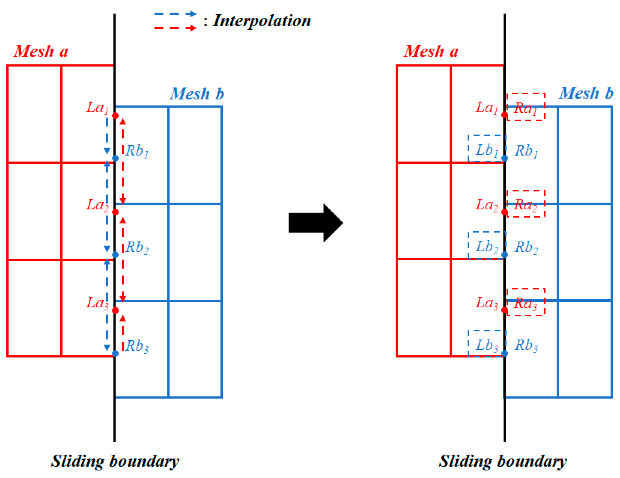
To accurately simulate the flow characteristics and aerodynamic performance of vertical axis wind turbines, this paper developed sliding mesh technology in the CFD solution program HUNS3D. To achieve communication of calculation data on both sides of the sliding boundary, this paper adopts the sliding mesh algorithm strategy shown in Figure 2. Taking surface element as an example: the closest surface element on the other side of the sliding boundary is used as the contribution element, and the flow field values of the contribution element and all adjacent surface elements are used as the interpolation basis to obtain the flow field values on the outer side of the sliding surface , and then proceed with subsequent flux calculations.
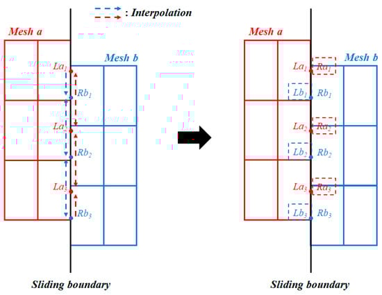
Figure 2.
Sliding mesh strategy.
2.2. Turbulence Modeling
2.2.1. Shear Stress Transport Model
For turbulence closure, this paper uses the k-ω Shear Stress Transport (SST) model and its corresponding DES method. The k-ω SST model is a two-equation turbulence model proposed by Menter et al. [53]. The k-ω SST model consists of two partial differential transport equations that describe turbulent kinetic energy and turbulent energy dissipation. Its differential form is as follows:
where k is the turbulent kinetic energy, is the velocity component in the direction , is turbulent eddy viscosity coefficient, is the vorticity magnitude, and are the model constant related to the destruction term and its modification, respectively. , , , , , are the specific dissipation rate, molecular viscosity, model constant related to the diffusion of and , model constant related to the production of ω, empirical constant, respectively.
After calibrating the empirical coefficients in the above model equations, the transition and fusion of the k-ε model and k-ω model were implemented in the following way:
where , ,
, , , , are the auxiliary variables for blending function, and d is the distance to the nearest wall, is empirical constant, and is the cross-diffusion term coefficient. The details of the terms and constants in the above model equations can be found in ref. [53].
2.2.2. Improved Delayed Detached Eddy Simulation
The IDDES method [23] is a high-fidelity CFD approach that has been widely employed for simulating various types of complex flows. By integrating Wall-modeled LES with the DDES framework, the IDDES method effectively addresses issues such as log-layer mismatch and grid-induced separation that are commonly observed in traditional DES and DDES models. This enables a more accurate prediction of flow separation regions and near-wall behaviors. In the SST-IDDES formulation, the dissipation term in Equation (2) is modified by introducing a hybrid length scale , given by
The IDDES mixing length is written as
where the and the are the length scales of the RANS and the LES, respectively. They are defined as
where is a constant in the k-ω SST model, is the grid scale, is a constant, d is the distance to the nearest wall, the grid maximum scale is , and . The definition of the blending function and elevating function can be found in ref. [23].
2.3. Geometry and Flow Condition
This paper uses simplified symmetrical blade VAWT and J-shaped VAWT as geometrical models, as shown in Figure 3. Since this paper primarily investigates the effect of airfoil shape on the performance of the VAWT, the effects of the shaft and the support arm are ignored. Both the symmetrical blade VAWT and the J-shaped VAWT are based on the NACA0015 airfoil design, with specific parameters shown in Table 1. In this paper, the symmetrical blade is referred to as the S-shaped blade, and the J-shaped blade is designed by eliminating one side of the S-shaped blade from the maximum thickness [39], as shown in Figure 1.
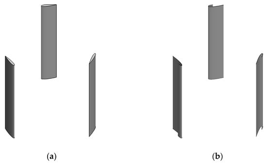
Figure 3.
Geometric model of VAWT: (a) S-shaped VAWT, (b) J-shaped VAWT.

Table 1.
Specific parameters of VAWT.
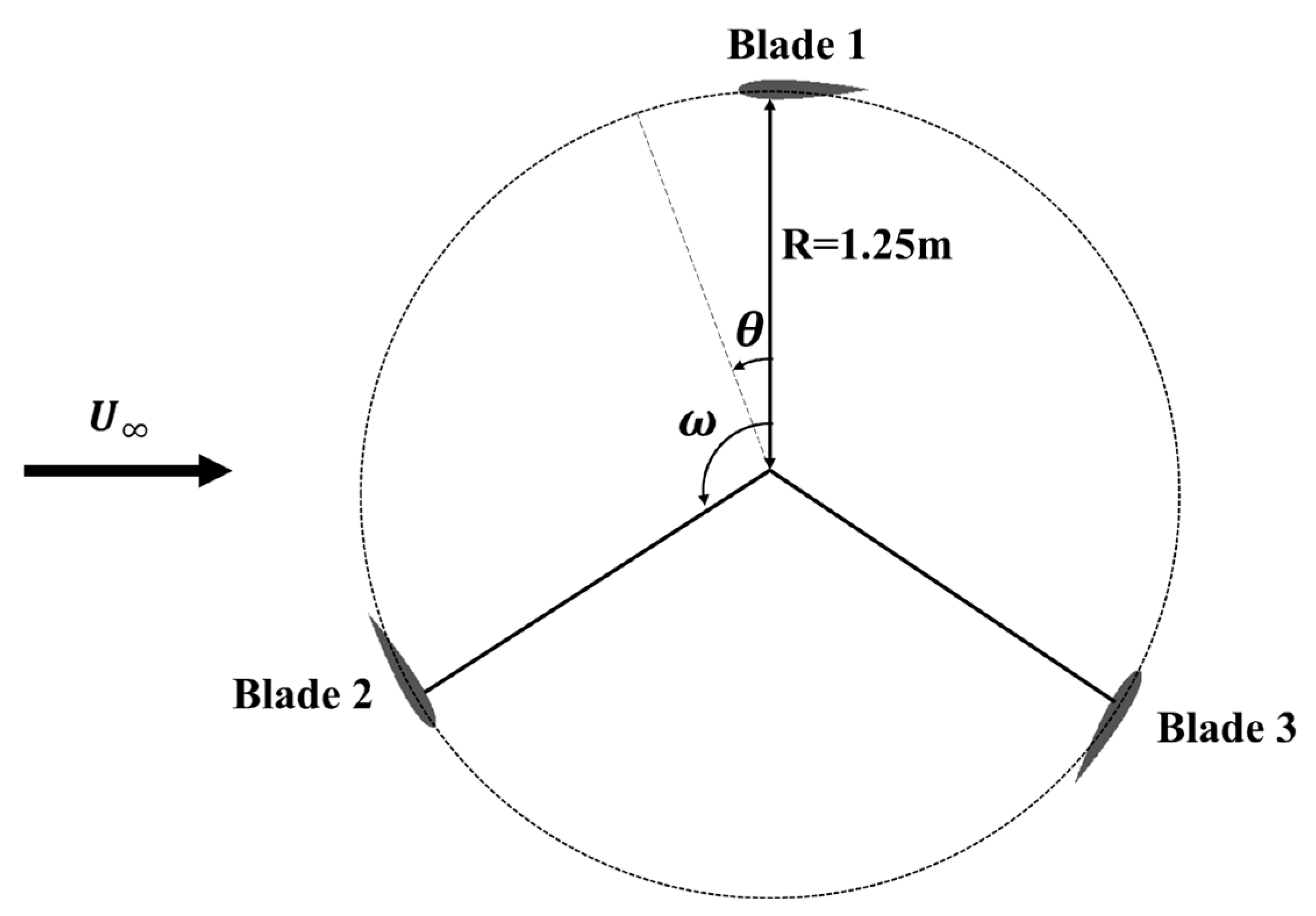
The top view of the S-shaped VAWT is shown in Figure 4, the free incoming flow direction, the blade’s azimuth angle and the rotor’s angular velocity are also given in Figure 4. In order to describe the motion process of the wind turbine in a simple way, the blade motion in this paper is divided into four regions: upwind (), leewind (), downwind (), and windward () [54]. This paper examines four-blade TSRs, designated 1, 1.6, 1.8, and 2, respectively. The TSR can be defined as , where D is the turbine diameter and is the incoming flow velocity. In this paper, the is maintained at a constant value of 10 m/s. The flow density is 1.225 kg/m3, the dynamic viscosity is 1.789 × 10⁻⁵ kg/(m·s), and the Reynolds number is about Rechord = 2.7 × 10⁵ ~ 5.5 × 10⁵.

Figure 4.
Top view of the S-shaped VAWT model.
2.4. Computational Mesh and Numerical Setup
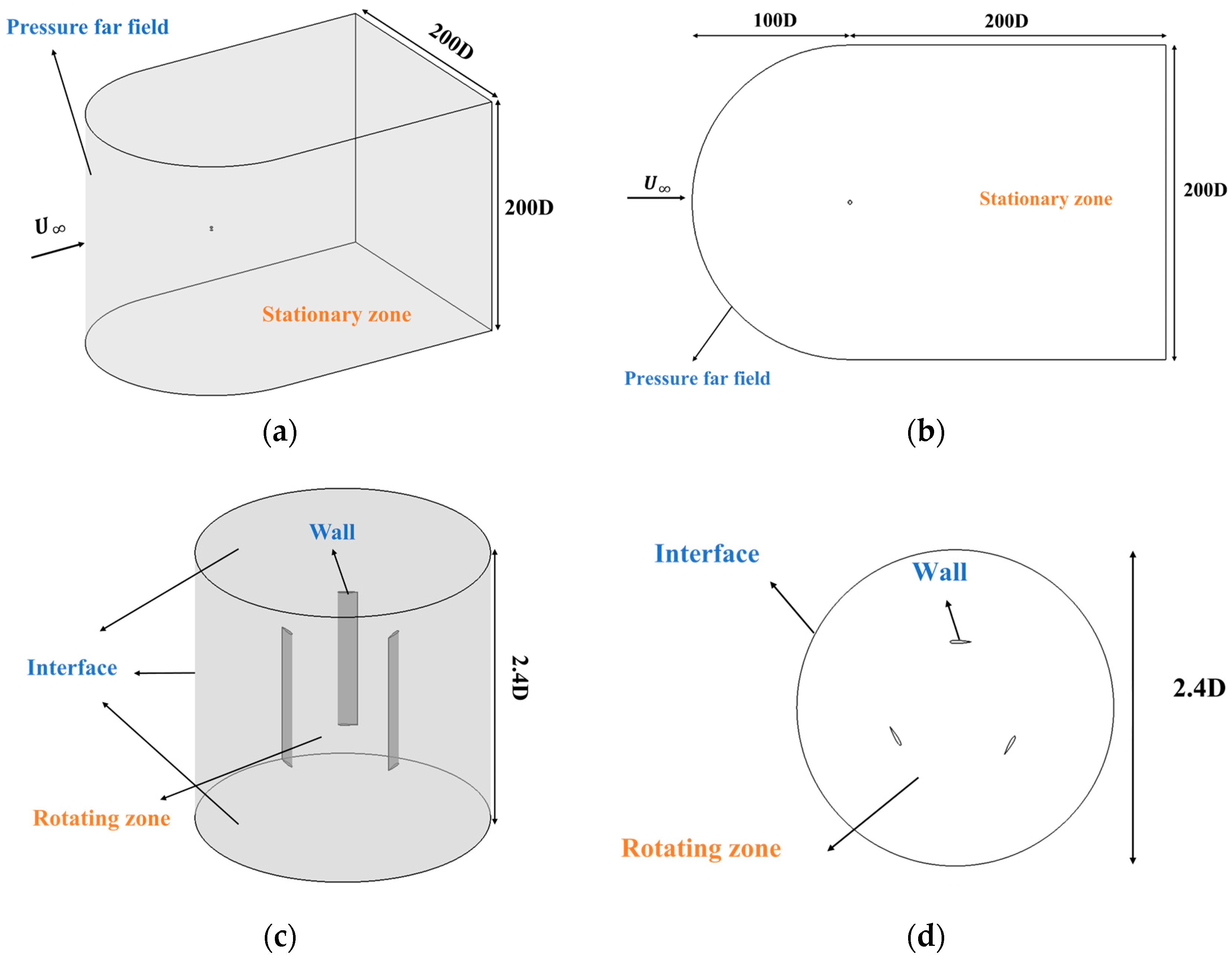
The computational domain of this paper is shown in Figure 5. It consists of a rotating zone and a stationary zone. The rotating zone has a diameter and height of 2.4D. The stationary zone consists of a semi-cylinder and a square, both with diameters and lengths of 200D. The far-field boundary condition uses a non-reflecting pressure far field. The intersection of the rotational and stationary domains uses a slip interface, and the blades use a viscous wall boundary condition.
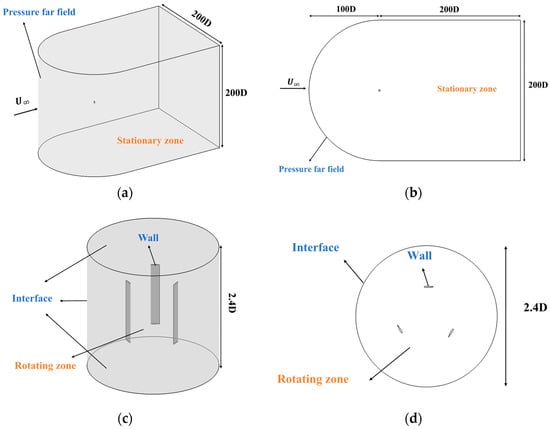
Figure 5.
Computational domain: (a) 3D view of the stationary zone, (b) top view of the stationary zone, (c) 3D view of the rotating zone, and (d) top view of the rotating zone.
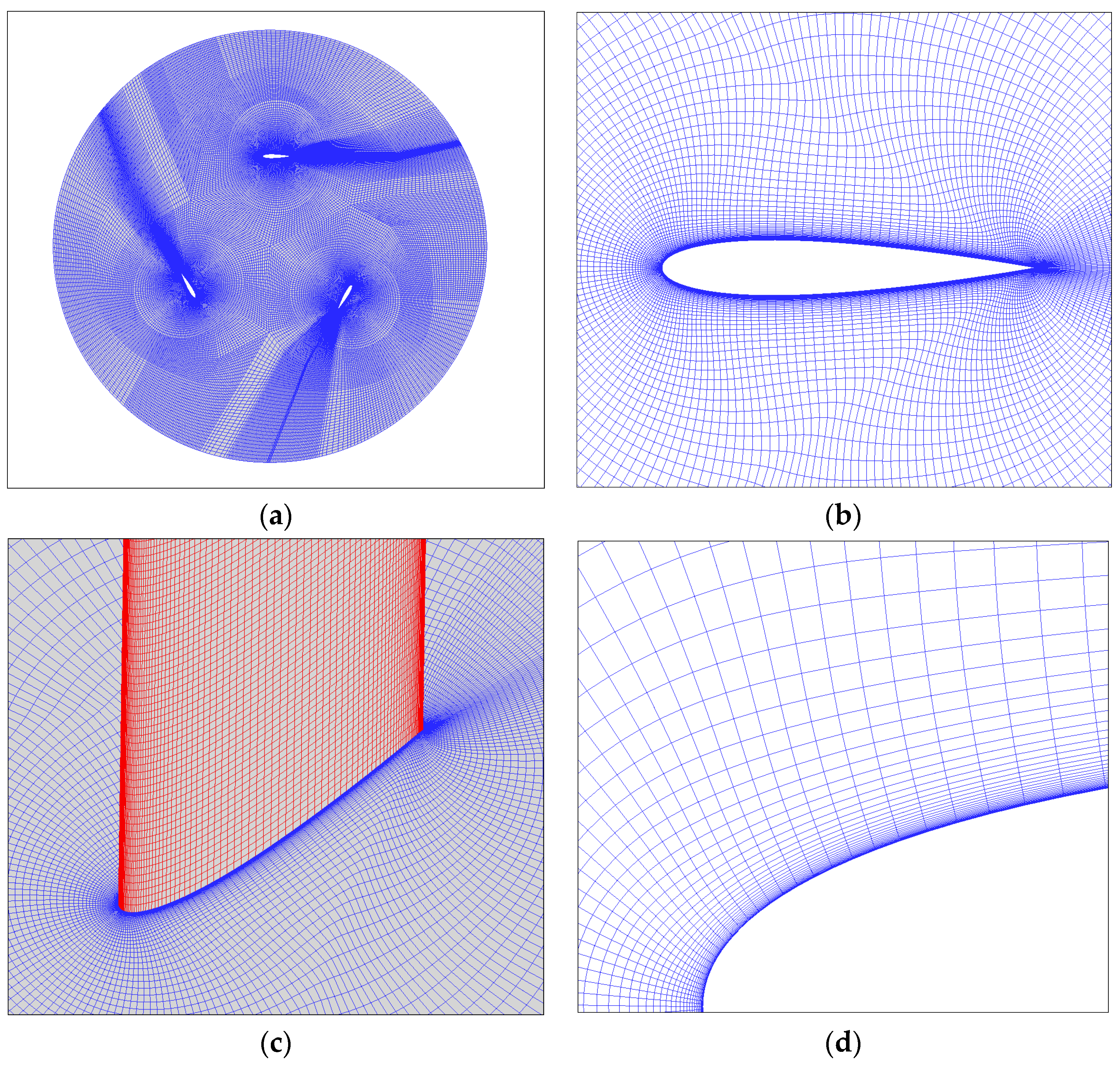
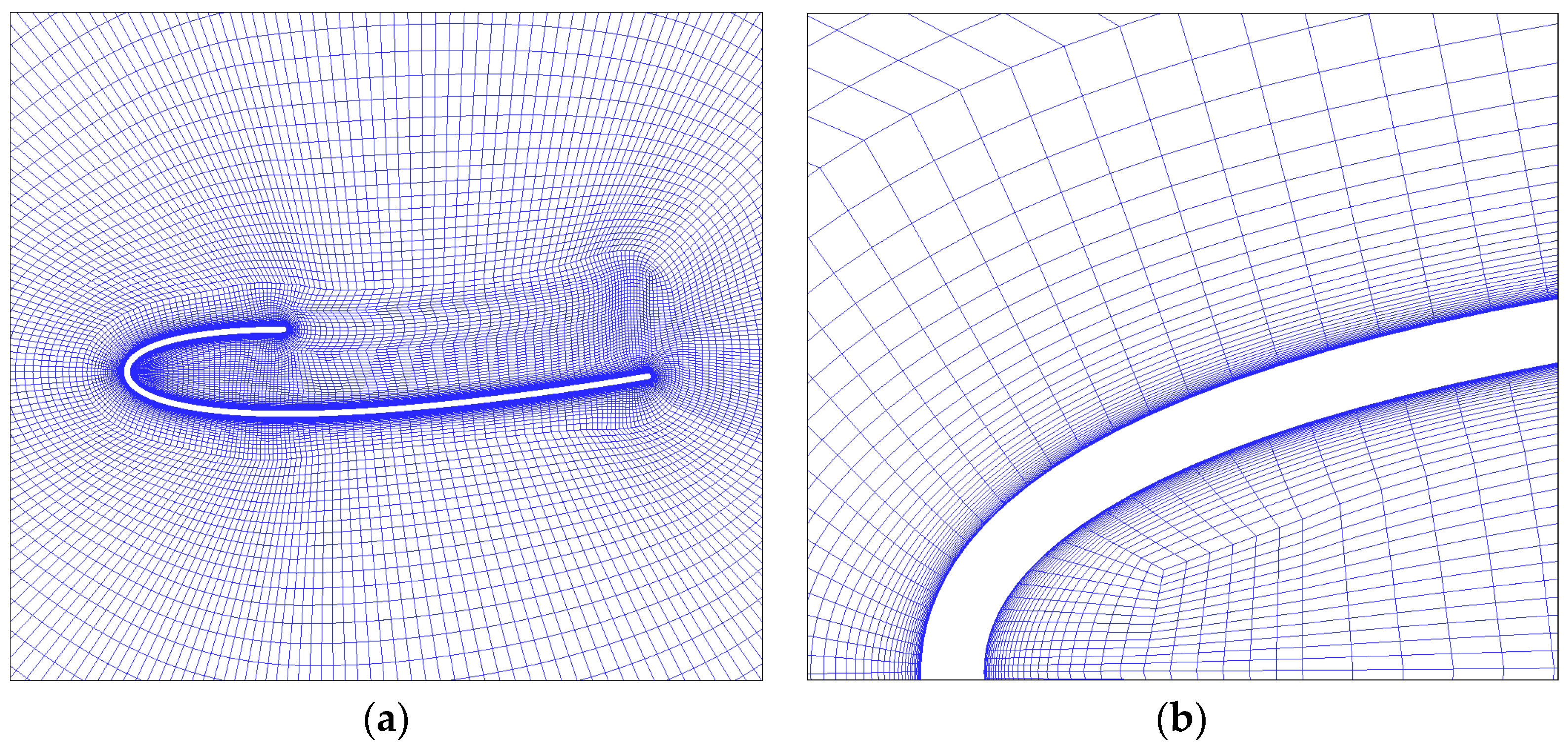
Figure 6a shows the mesh structure at the rotating zone, and it has a fully structured mesh with refinement in the wake region to capture the complex flow structure. Figure 6b shows the grids around the blade, with 240 × 200 grid nodes in circumferential and spanwise. To ensure accurate simulation of the boundary layer, the height of the first layer is m to meet the requirement of the SST-IDDES model, with a growth rate of 1.2. The mesh topology of the J-shaped blade is shown in Figure 7, with the same boundary layer setup as the S-shaped blade, and it has 340 × 200 grid nodes in circumference and spanwise. The S-shaped VAWT has 32,666,558 meshes, and the J-shaped VAWT has 34,184,216 meshes. The grid resolution employed in this study is deemed sufficient for conducting the IDDES simulations based on comparative evaluations with previous studies [55,56,57]. Specifically, ref. [55] investigated the VAWT wake using overlapping grids, and performed grid independence analysis with six sets of grids, the densest of which contained approximately 7 million cells. In contrast, the present study utilizes grids exceeding 30 million cells, providing a much finer resolution. Ref. [56] adopted structured grids for VAWT wake simulations, achieving grid independence with their densest grid at 4.1 million cells, again considerably lower than the current study. Additionally, ref. [57] carried out a detailed grid convergence study using the Grid Convergence Index (GCI) method, where grid sizes corresponding to chordwise element lengths of 6.5%, 2.5%, and 1.5% of the chord were analyzed. The corresponding grid size is 2.8 million, 16.9 million, and 55.1 million, respectively. Their results indicate convergence when the element size is 2.5% of the chord length. In the present study, the maximum chordwise element size was maintained below 2.5% of the chord length, satisfying the established convergence criteria. Therefore, based on mesh size, mesh resolution, and convergence criteria, the present grid configuration was confirmed to be sufficiently fine for accurate IDDES simulations of VAWTs.
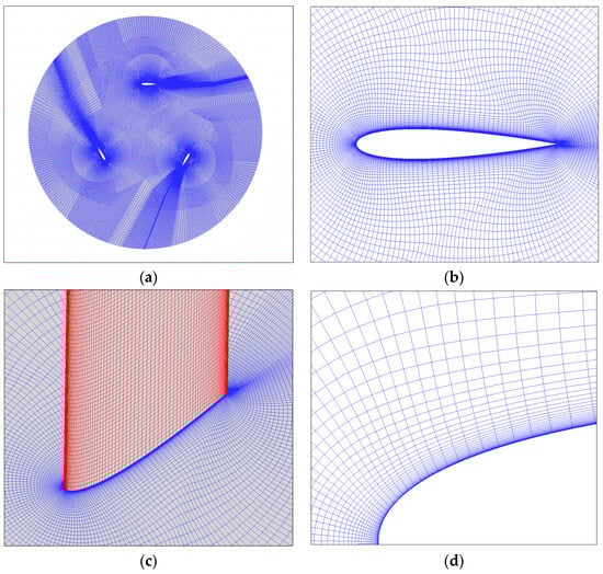
Figure 6.
Rotating zone grid topology: (a) grids at the rotating zone, (b) grids around the blade, (c) grids near the blade (the blade grids is stained with red), (d) boundary layer grids.
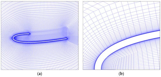
Figure 7.
Grids around the J-shaped blade: (a) grids on blade surface, (b) boundary layer grids.
To rapidly diminish the influence of initial conditions, unsteady computations begin with the steady-state solution as the initial condition. The steady case is simulated using the SST-RANS model, whereas the SST-IDDES model is applied for the unsteady case. The unsteady time step interval corresponds to a rotor rotation of 3°, which has been validated as sufficient for simulating VAWT [19,42]. Each time step undergoes up to 500 iterations to ensure the residual is sufficiently small. Figure 8 shows the variation in the instantaneous torque coefficient of one S-shaped blade with a time step at TSR = 1.6. The peak torque coefficient values at the third and fourth revolutions are 0.3647 and 0.3623, respectively, resulting in a relative error of approximately 0.66%. This error falls within the acceptable threshold (less than 1%) based on the convergence criterion proposed in ref. [24]. Therefore, the data from the fourth revolution are utilized for the aerodynamic performance analysis in this study. All simulations use 960 partitions for MPI-parallel computing to speed up the calculation speed, which takes about 46 h to calculate four revolutions. The numerical setup for the current calculations is summarized in Table 2.
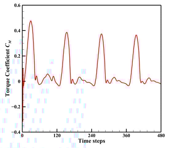
Figure 8.
Variation in the instantaneous torque coefficient of one S-shaped blade with a time step at TSR = 1.6.
Table 2.
Numerical setup.
2.5. Validation
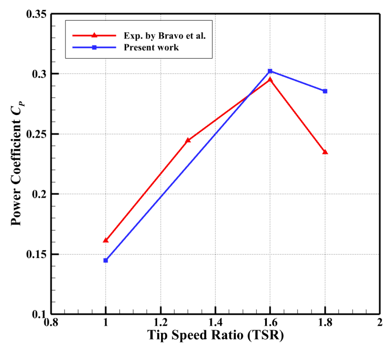
The power coefficient serves as a key parameter in evaluating the performance of the VAWT and is defined as
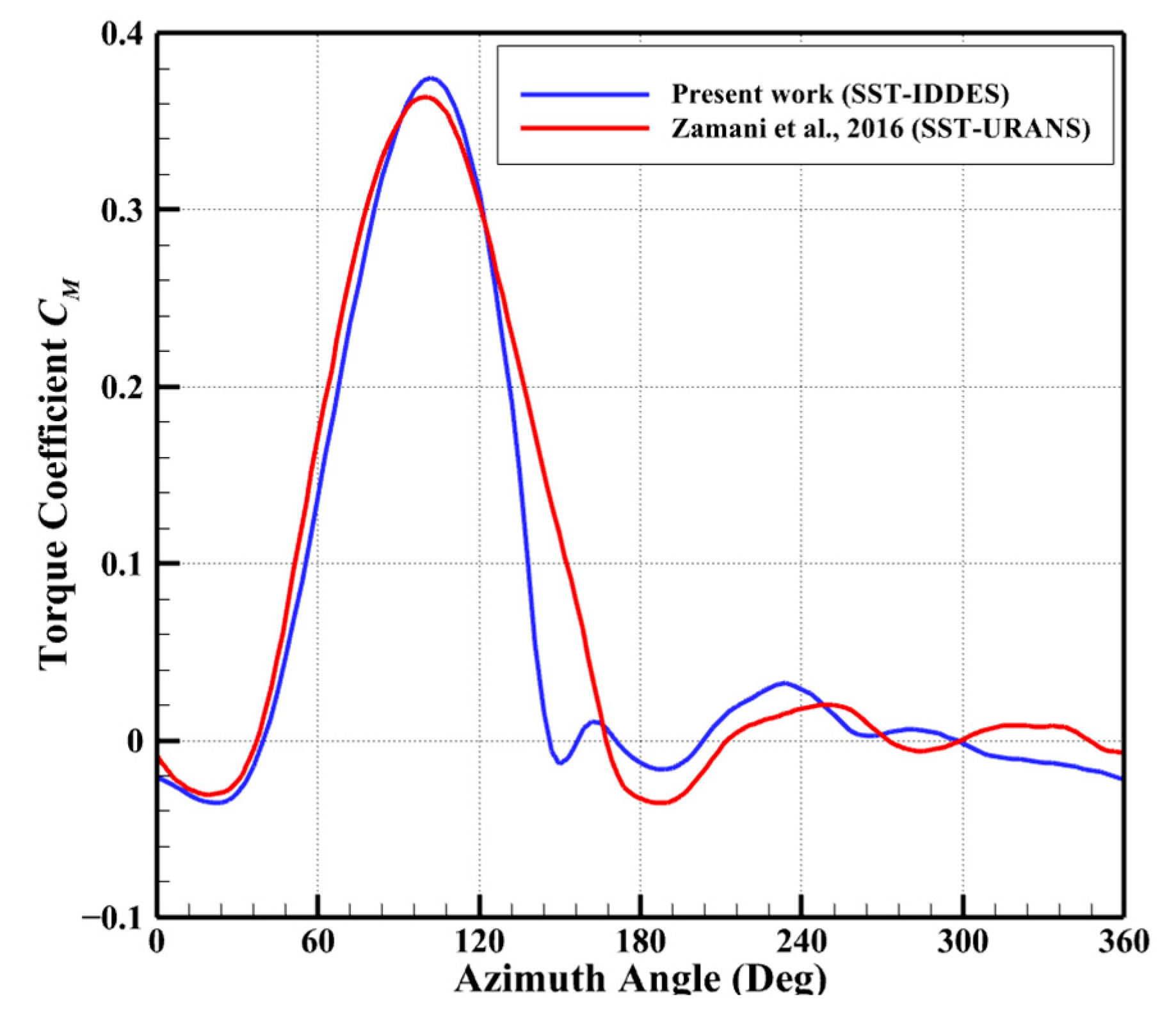
where and A are the rotor torque, rotational angular velocity, incoming flow density, incoming flow velocity, and swept area of the rotor, respectively. To validate the current numerical findings, computed power coefficient CP values were compared with experimental data from Bravo et al. [58], as shown in Figure 9. It can be seen that the variation in Cp with TSR obtained by the current numerical method is in good agreement with the experimental values. However, when TSR = 1.8, the numerical results have a large error with the experimental values, which is due to the fact that the numerical simulation does not consider the friction and the aerodynamic loss of the strut [59]. Since the experiments only have data on average power coefficient and TSRs, Figure 10 shows the torque coefficient of a single blade rotating for one cycle at TSR = 1.6 and compares it with the results of Zamani et al. [40]. The results show better agreement between the two numerical simulations, but discrepancies remain between the maximum and minimum torque values. These differences primarily stem from Zamani et al. [40] using the URANS model, while the current study employed the IDDES model.

Figure 9.
Comparison of the present work and experimental results [58].
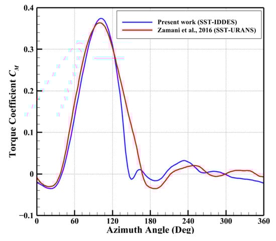
Figure 10.
Comparison of the present work and Zamani et al. [40] results for the torque coefficient at TSR = 1.6.
3. Results and Discussion
The magnitude of the torque coefficient directly affects the of the VAWT, and its variation is critical to the aerodynamic performance of the wind turbine. The torque coefficient is defined as
Figure 11 compares the time-averaged of the S-shaped and J-shaped VAWTs over one week of rotation at different TSRs. It can be observed that the of both types of VAWTs initially increased with TSR before peaking at TSR = 1.6, after which it decreased. Furthermore, the of the J-shaped VAWT was higher than that of the S-shaped VAWT at low (TSR = 1) and medium (TSR = 1.6) TSRs, but became lower at a high TSR (TSR = 2). To understand the underlying causes of these variations, this study will conduct a comprehensive analysis of the aerodynamic performance of the two VAWTs at different TSRs. Specifically, the investigation will focus on aerodynamic loads, pressure distributions, and flow field structures to provide deeper insights into the mechanisms influencing VAWT efficiency.
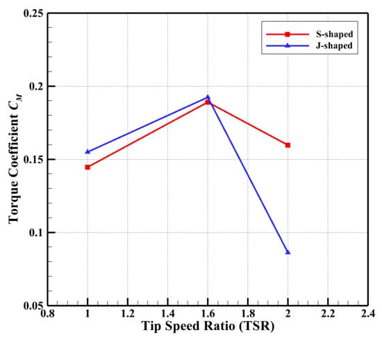
Figure 11.
Comparison of the time-averaged power coefficient.
3.1. Aerodynamic Loads
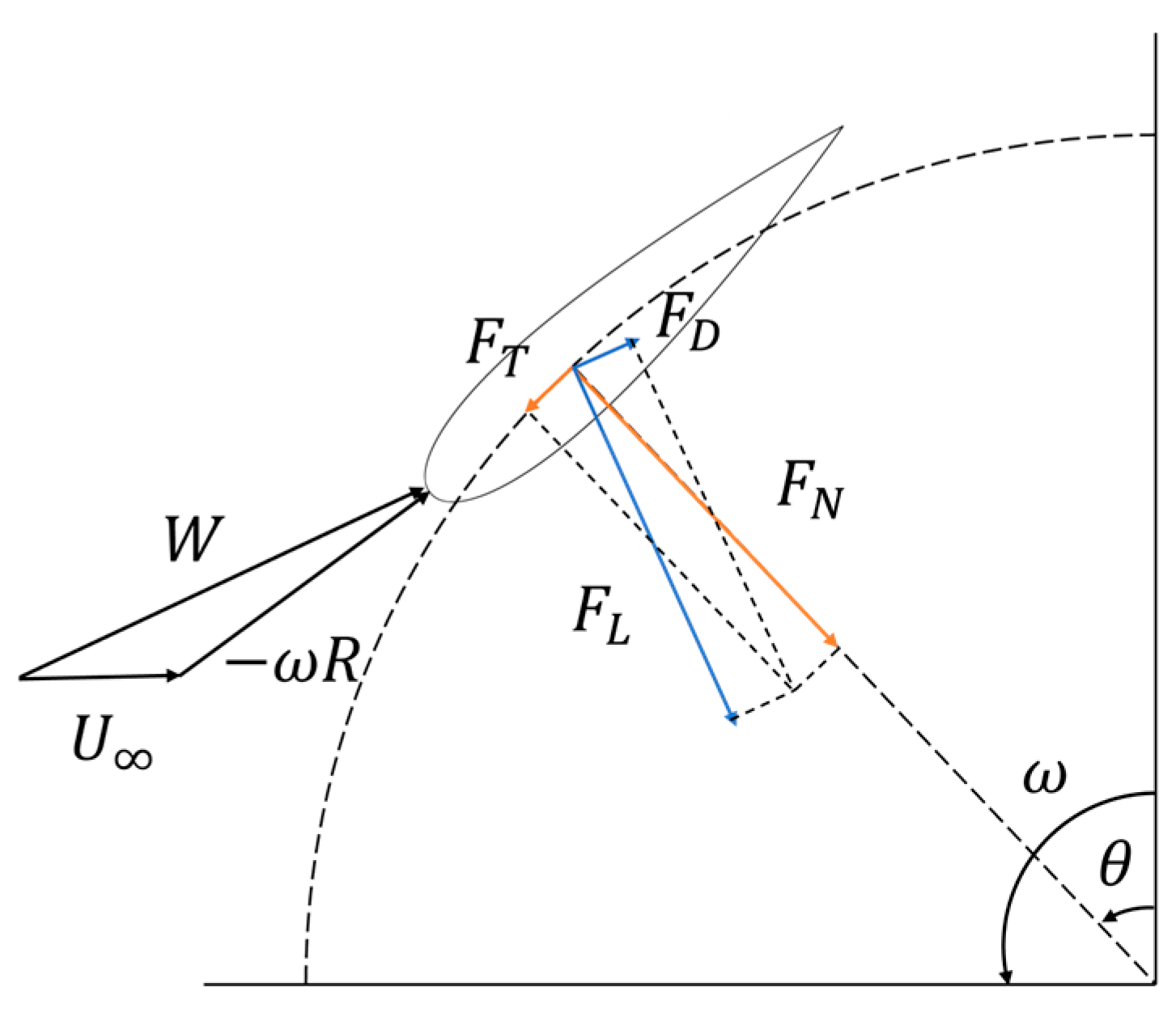
The measurement of aerodynamic load is of paramount importance in the assessment of the aerodynamic performance of a wind turbine. The force exerted by the wind turbine blade is illustrated in Figure 12. and
are the tangential force, normal force, lift and drag, respectively. In which the tangential force is the main force to provide the rotational torque of the rotor. This section illustrates the variations of force coefficients for the two VAWTs at low, medium, and high TSRs.
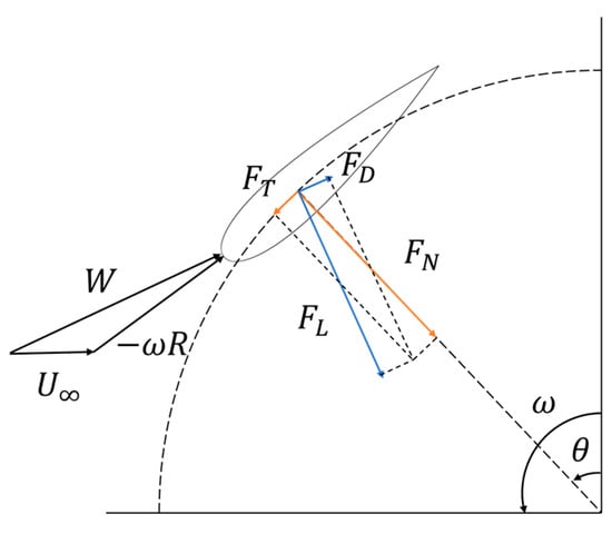
Figure 12.
The forces applied to the blade.
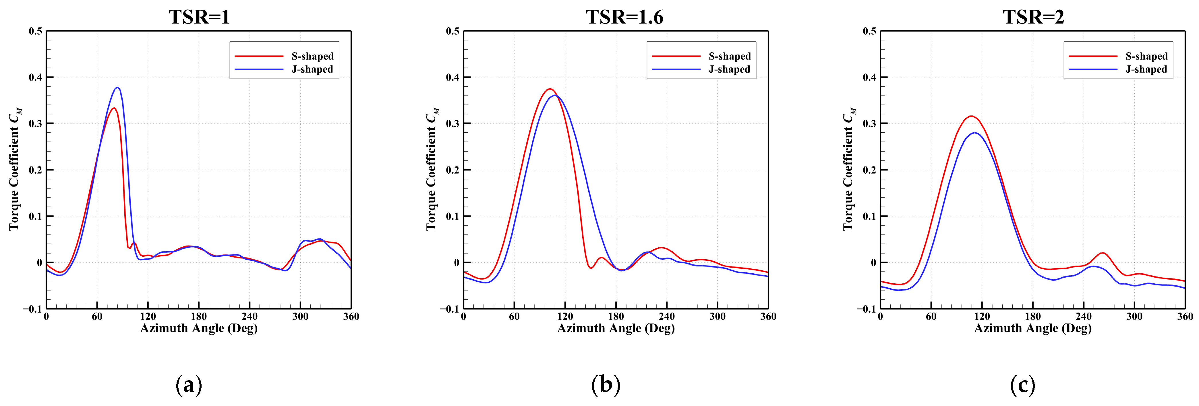
Figure 13 illustrates the variations of the torque coefficient CM of a single blade with azimuth angle at different TSRs. It can be observed that the J-shaped blade does not significantly affect the overall distribution of the CM over one rotation cycle. However, its effect on the CM varies across different TSRs. At a low TSR, the CM of the J-shaped blade is consistently higher than that of the S-shaped blade in most of the upwind region. The maximum value of the CM for the J-shaped blade is 0.3787, which occurs at an azimuth angle of 84°. In contrast, the maximum value of CM for the S-shaped blade is 0.3334, which occurs at an azimuth angle of 80°. The J-shaped blade delays the occurrence of the peak CM and increases its magnitude, enhancing the aerodynamic performance of the wind turbine in this region.
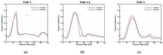
Figure 13.
The variations in the torque coefficient versus azimuthal angle at different TSRs: (a) TSR = 1, (b) TSR = 1.6, (c) TSR = 2.
At a medium TSR, the time-averaged torque coefficient CM of the J-shaped blade was 0.1923, slightly higher than the CM of the S-shaped blade, which was 0.1889. As shown in Figure 13b, in most leewind regions (), the CM of the J-shaped blade was higher than that of the S-shaped blade. Notably, the minimum CM for the S-shaped blade was −0.013 at = 150°, while the CM for the J-shaped blade is 0.140, significantly higher. Furthermore, the azimuth angle at which the CM of the J-shaped blade starts to decrease also lags behind that of the S-shaped blade, similar to observations at low TSR. However, in all other regions, the CM of the J-shaped blade is lower than that of the S-shaped blade. Consequently, the power coefficient of the J-shaped blade is only slightly higher than that of the S-shaped blade.
At a high TSR, the time-averaged torque coefficient CM of the J-shaped blade was considerably lower than that of the S-shaped blade. As shown in Figure 13c, at all azimuth angles, the CM of the J-shaped blade was lower than that of the S-shaped blade. In most leewind regions, the CM of the J-shaped blade experienced a smaller reduction than in other regions. This indicates that the J-shaped blade plays a positive role in this region, but not enough to counteract its negative effect. Consequently, the time-averaged torque coefficient of the J-shaped blade is significantly reduced.
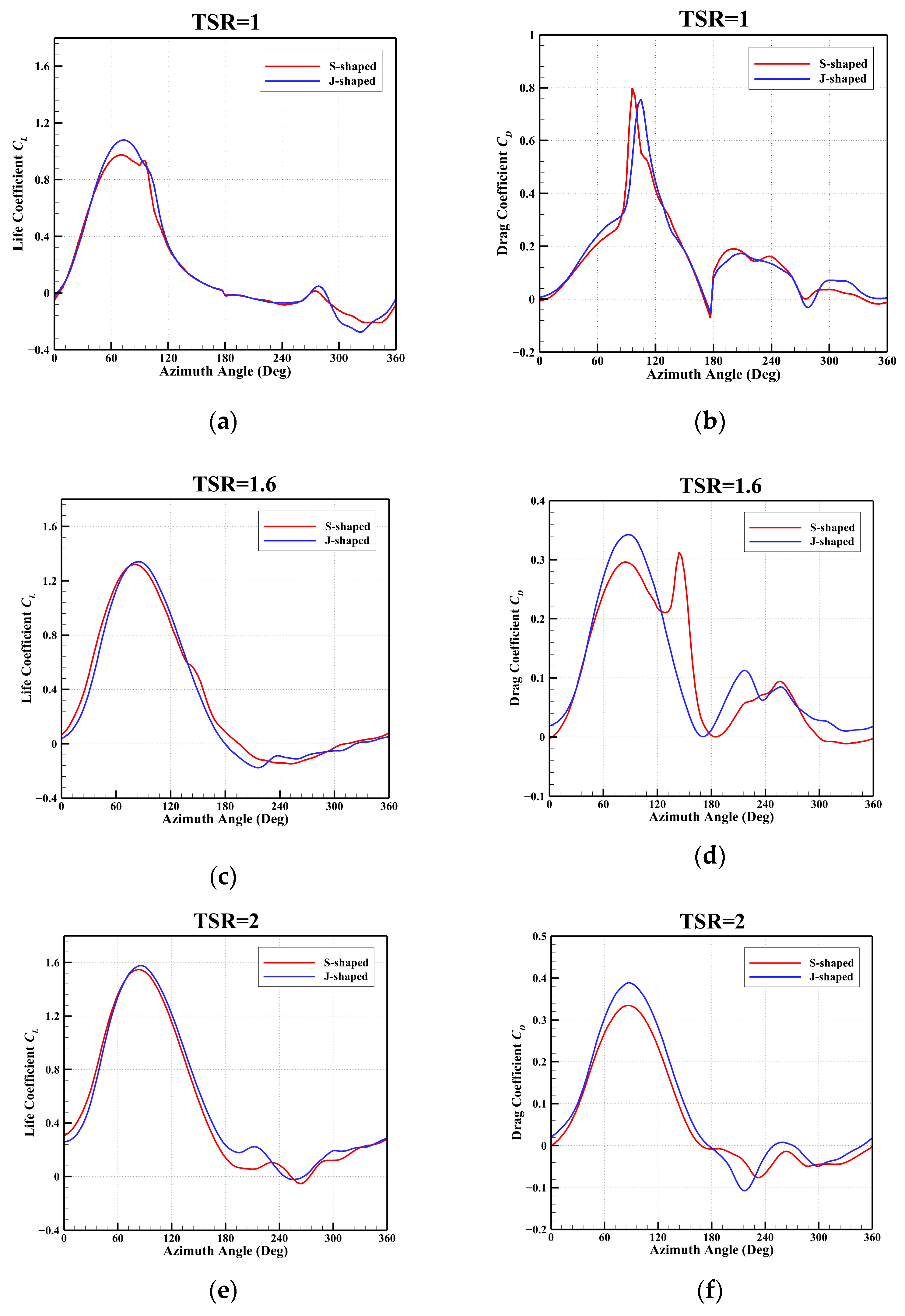
Furthermore, the variations in the lift coefficient CL and the drag coefficient CD provide additional insight into torque fluctuations. Figure 14 illustrates the variations in the CL and the CL with azimuth angle for both blade types at different TSRs. As depicted in the figure, the general trend of the CL for both blades remains consistent. The CL of the blade increases linearly with azimuth angle as the blade begins to rotate, and then decreases rapidly after reaching the maximum value due to dynamic stall. At a low TSR, near the peak (), the CL of the J-shaped blade is higher than that of the S-shaped blade. The peak CL for the J-shaped blade was 1.0790, which is 11% higher than that of the S-shaped blade (0.9738). Moreover, the peak CL for the J-shaped blade occurs at a later azimuth angle () than for the S-shaped blade (). This indicates that the J-shaped blade effectively delays dynamic stall. At medium and high TSRs, the maximum CL value of the J-shaped blade is slightly higher, and the azimuth angle at which dynamic stall occurs lags behind that of the S-shaped blade. This suggests that the J-shaped blade continues to contribute to delaying dynamic stall at medium and high TSRs.
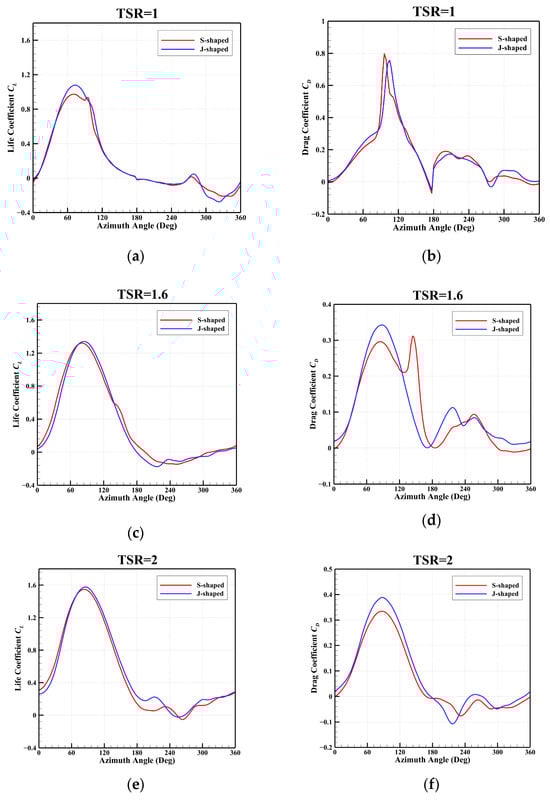
Figure 14.
Variations in the lift coefficient and the drag coefficient versus azimuthal angle at different TSRs: (a) CL at TSR = 1; (b) CD at TSR = 1; (c) CL at TSR = 1.6; (d) CD at TSR = 1.6; (e) CL at TSR = 2; (f) CD at TSR = 2.
The fluctuation in the drag coefficient for both blade types is particularly pronounced. As shown in Figure 14b, at low TSR, the CD of the S-shaped blade increases linearly after . In contrast, the increase in CD for the J-shaped blade is delayed relative to the S-shaped blade, and its maximum CD is lower. This further supports the conclusion that the J-shaped blade enhances dynamic stall performance. However, at medium and high TSRs, the peak CD of the J-shaped blade was significantly higher than that of the S-shaped blade, likely due to its unique geometric configuration.
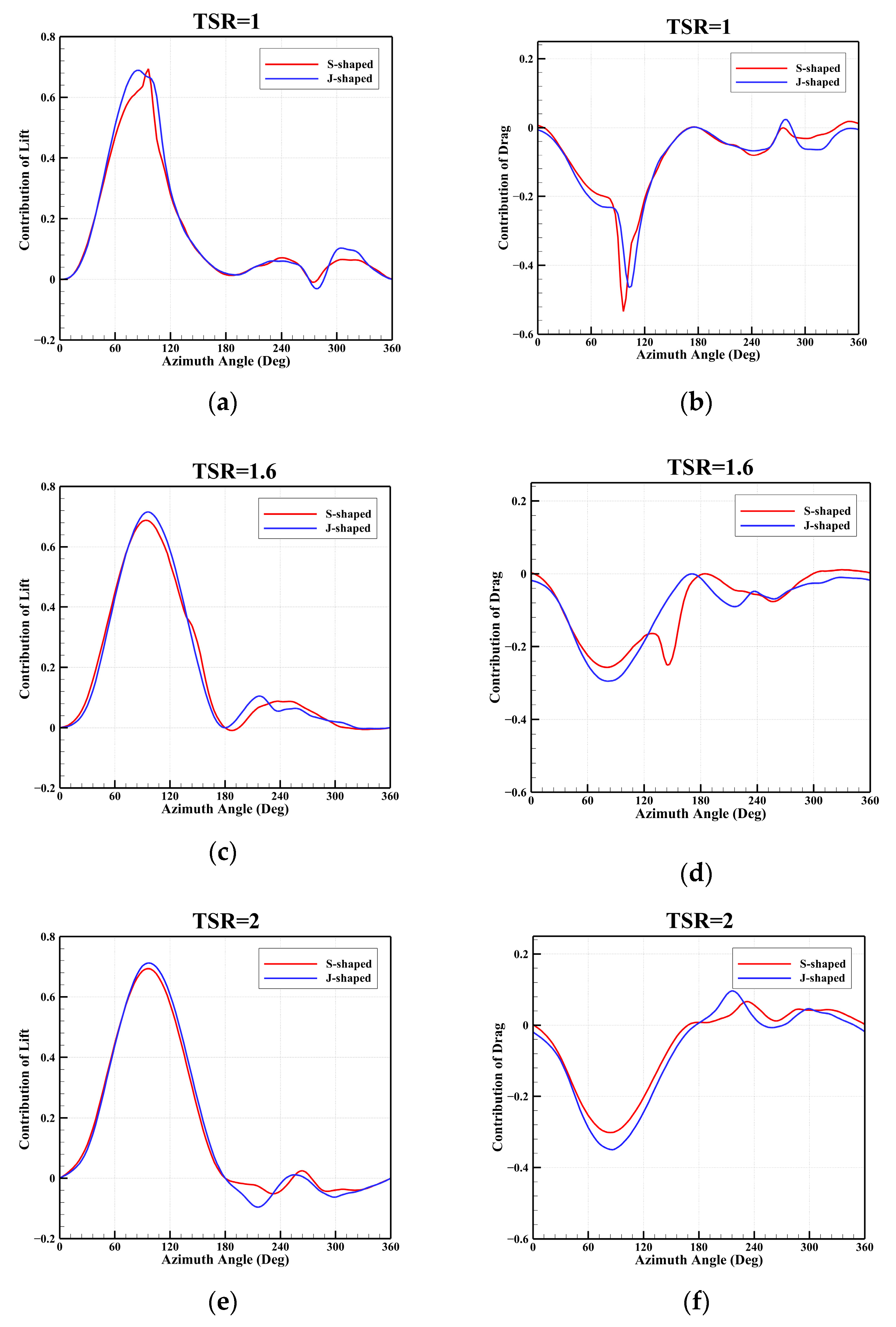
Since the pitch angle of the wind turbine in this study was 0°, the tangential force on the blade served as the primary contributor to the torque. To further investigate the influence of the J-shaped blade on the torque coefficient, the lift and drag of the blades were projected along the tangential force direction. This allowed for an evaluation of their respective contributions to the tangential force. Figure 15 presents the variations in the contribution coefficients of lift and drag to the tangential force of the wind turbine blade with azimuth. The results indicate that the lift force contributed most of the tangential force, while the drag force had a relatively minor positive contribution at three TSRs.
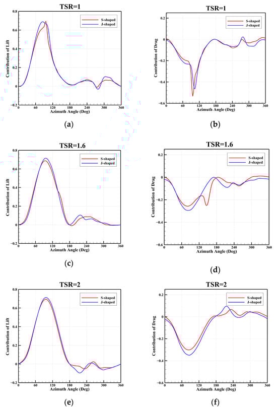
Figure 15.
Variations in the contribution of lift and drag to the tangential force versus azimuthal angle at different TSRs: (a) lift at TSR = 1; (b) drag at TSR = 1; (c) lift at TSR = 1.6; (d) drag at TSR = 1.6; (e) lift at TSR = 2; (f) drag at TSR = 2.
At a low TSR, the J-shaped blade exhibited a higher positive lift contribution and a smaller negative drag contribution compared to the S-shaped blade in the dynamic stall region. In other regions, the lift and drag contributions were similar for both blade types. As a result, the J-shaped blade generated a greater tangential force, resulting in a higher torque coefficient at a low TSR.
At medium TSR, the J-shaped blade maintained a greater positive lift contribution in most upwind regions and certain leeward regions relative to the S-shaped blade. Conversely, the drag contribution coefficient alternated between the two blade types with changing azimuth angles, resulting in little difference in their time-averaged drag contribution.
At high TSR, since dynamic stall is no longer a major issue, the lift-enhancing effect of the J-shaped blade was less significant. Consequently, the positive contribution of lift to the tangential force was nearly equal for both types of blades. However, due to the inherent geometric design defect of the J-shaped blade, increased drag introduced a greater negative contribution. This resulted in a substantially lower time-averaged torque coefficient for the J-shaped VAWT compared to the S-shaped VAWT at high TSR.
It is important to note that the design principle of the J-shaped blade is to leverage both lift and drag forces to enhance the torque coefficient at low TSR [40]. However, in this study, while the J-shaped blade increased resistance across all TSRs, this additional resistance did not positively contribute to the tangential force. Instead, it imposed a greater negative contribution. The increase in the torque coefficient of the J-shaped blade can be attributed to its effect on flow separation, which delays dynamic stall and results in a higher lift coefficient. Lift contributes more positively to the tangential force, leading to an increase in the torque coefficient. This conclusion is further substantiated by the flow structure analysis presented later in this study.
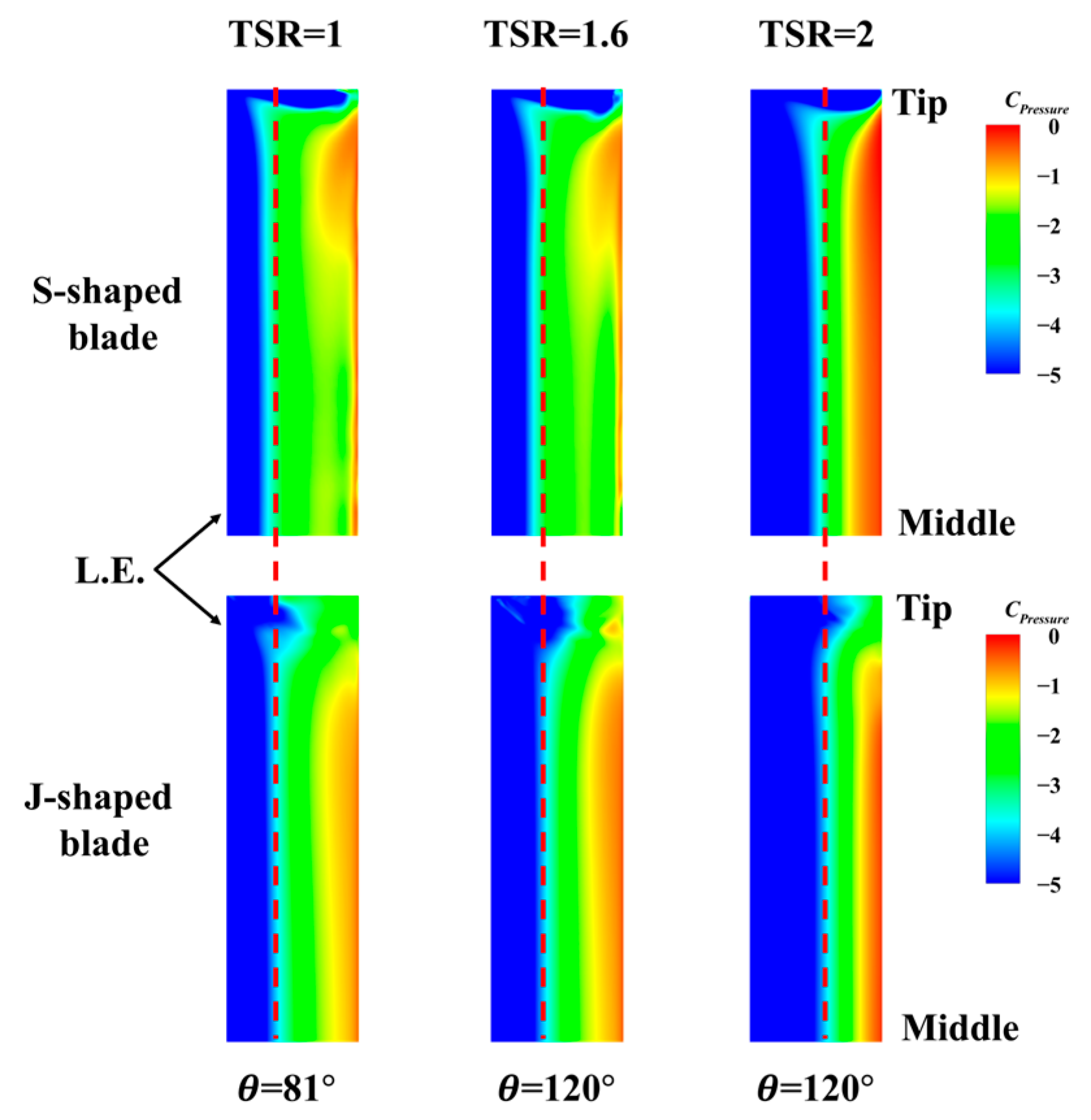
3.2. Pressure Distributions
The blade surface pressure distribution allowed for the visualization of the distribution of aerodynamic loads on the blade surface, as well as the reflection of the three-dimensional characteristics of the flow field along the spreading direction. To evaluate the impact of the J shape on the blade surface pressure distribution, this paper compares the suction surface pressure distribution (half mode) of two types of blades at the azimuthal angle where the J-shaped blade exhibits enhanced performance (i.e., the azimuthal angle where the lift is increased in comparison with that of the S-shaped blade), as illustrated in Figure 16. There was a notable disparity in the pressure distribution on the suction side between the two types of blades, with a more pronounced negative pressure zone at the leading edge of the J-shaped blades. This larger negative pressure zone on the suction side gives rise to a more substantial pressure differential between the pressure side and the suction side, which in turn leads to an augmentation in the lift coefficient.
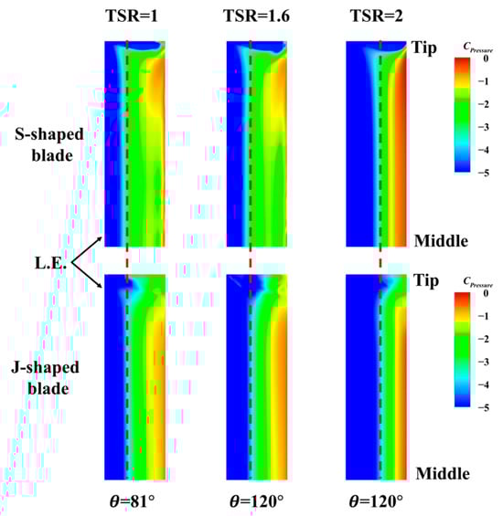
Figure 16.
Comparison of pressure coefficient distribution on the blade surface.
It is noteworthy that the S-shaped blade exhibited a distinctive suction zone at the tip [60], which generates a significant pressure differential between the root and the tip. This phenomenon promotes cross-flow at the blade surface, rendering the blade more susceptible to flow separation at subsonic speeds [61]. In contrast, J-shaped blades lack this suction region, resulting in a weaker surface cross-flow and reduced propensity for flow separation.
3.3. Flow Field Structures
The surface friction lines of wind turbine blades have the capacity to reflect the flow structure on the blade surface. Figure 17 presents the comparison of the limiting streamlines at with different TSRs. The limiting streamline visualization reflects the local wall shear stress direction and is an effective method to identify flow separation, attachment lines, and critical points on the blade surface. It can be observed that a distinct negative bifurcation line is present on all six blades, defining this line as a separation line [60]. A horizontal comparison reveals that the separation line gets closer to the trailing edge as the TSR increases. This suggests that at the same azimuth angle, higher TSR results in weaker flow separation and less severe dynamic stall.
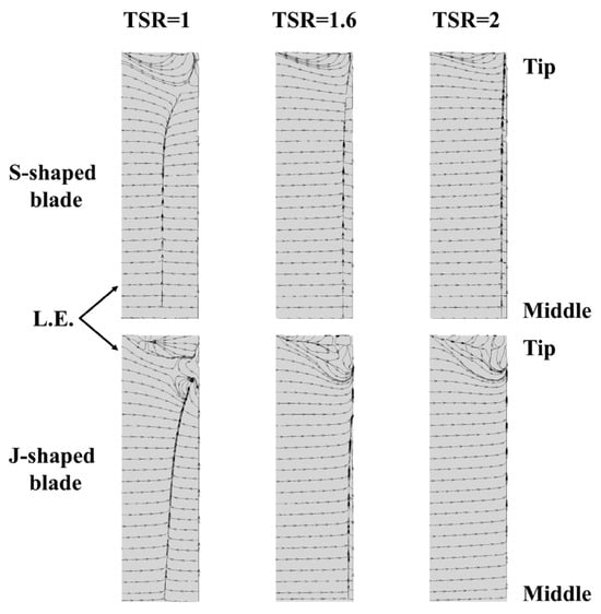
Figure 17.
Comparison of the limiting streamlines on blade surface at .
A longitudinal comparison reveals that at a given azimuth angle, the separation line of J-shaped blades is situated in closer proximity to the trailing edge, thereby indicating that J-shaped blades exert a suppressive effect on flow separation and can delay dynamic stall. It is noteworthy that the surface friction lines of the J-shaped blade exhibit increased turbulence at the tip, and the spreading region affected by the tip is larger, with a stronger three-dimensional effect. In particular, at a low TSR, the surface separation lines of the J-shaped blade displayed greater curvature in comparison to the S-shaped blade. This observation suggests that the enhanced three-dimensional effect at the tip of the J-shaped blade facilitated improved flow separation at the blade surface, as illustrated in the subsequent section.
The distribution of vortex systems around wind turbine blades is a determining factor in the pressure distribution on the blade surface. Consequently, the evolutionary characteristics of these vortex systems are critical for wind turbine aerodynamic loads. In this paper, the near-field vortex system is identified using the dimensionless vorticity and the Rortex identification method. The Rortex method has better performance in identifying the structure of the vortex system [62], and the Rortex iso-surface is defined as follows:
where r is the vortex core vector and R is the rotation strength around r. The vortex patterns presented in this paper are all the iso-surfaces of Rortex = 0.065, colored according to the corresponding dimensionless velocities . The dimensionless vorticity is defined as follows:
where is the physical vorticity, is the real physical length corresponding to the unit length of the grid, and is the sound speed. This paper uses the Z-component of to display two-dimensional vorticity distribution.
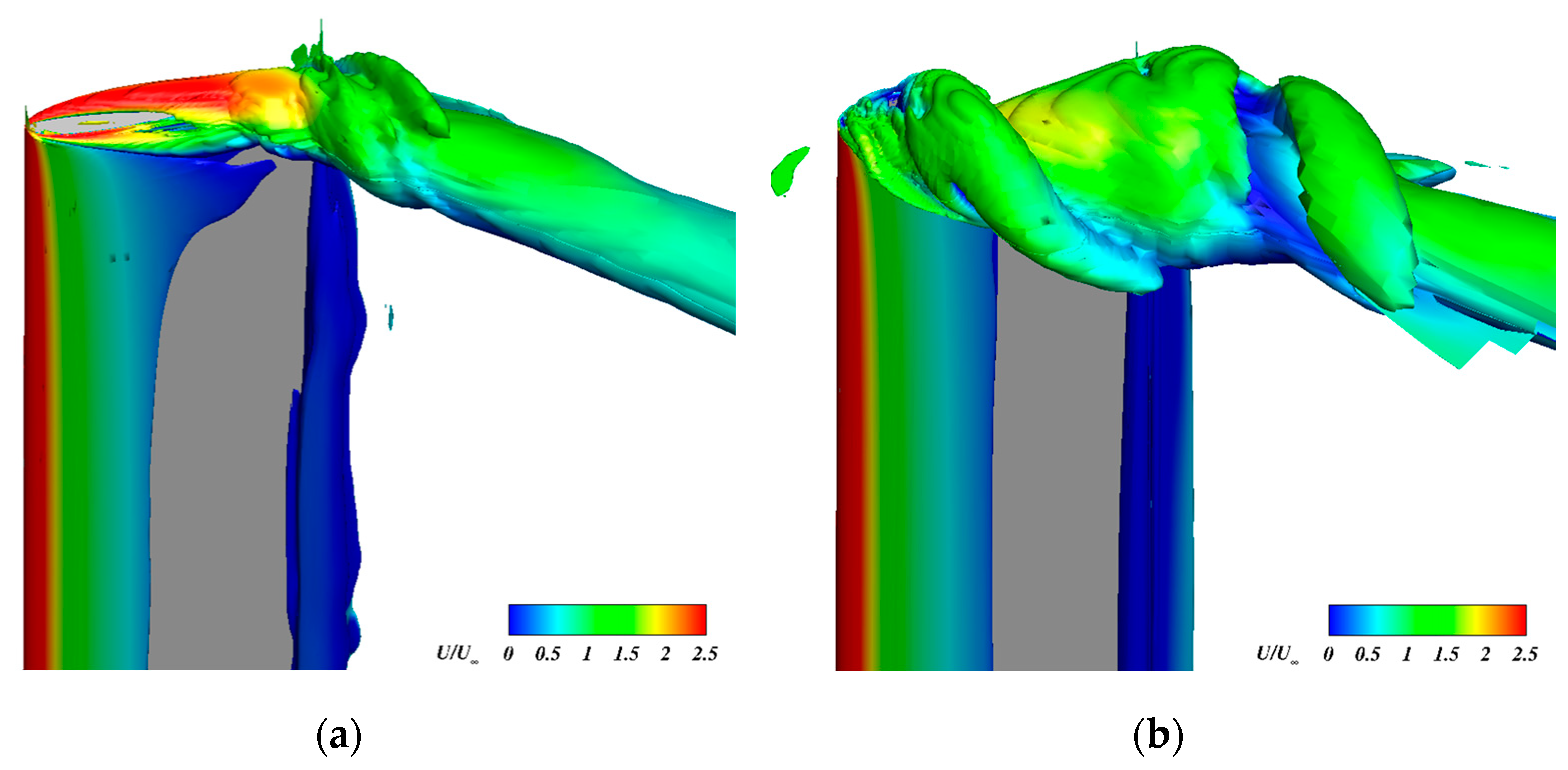
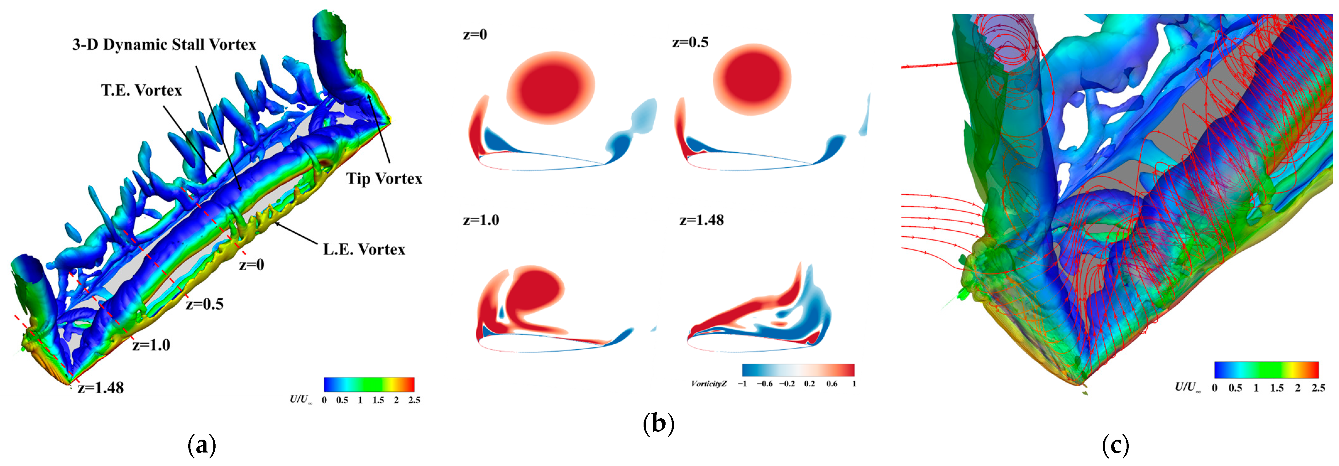
Figure 18 presents a comparison of the tip vortex of the two blade types at with low TSR. It can be observed that the vorticities captured in the concave region of the J-shaped blade escaped from the blade tip and combined with the tip vortex, thereby enhancing its strength. Consequently, the surface friction lines of the J-shaped blade exhibited a more pronounced three-dimensional effect in comparison to the S-shaped blade. Figure 19 illustrates the structure of the vortex system surrounding the S-shaped blade at with a low TSR, at which azimuthal angle the blade has already undergone a severe dynamic stall. As can be observed in Figure 19a, the complexity of the vortex system around the blade is primarily composed of a three-dimensional dynamic stall vortex, leading edge vortex, trailing edge vortex, and tip vortex. The tip vortex and dynamic stall vortex interact to form an -shaped vortex, which in turn gives rise to a strong three-dimensional effect in the local flow field [63]. Figure 19b provides a further illustration of the vorticity distribution at different sections. It can be observed that the dynamic stall vortex in the central section (z = 0) was the most pronounced, and the vortex strength diminished toward the blade tip. Figure 19c explains the reason for this phenomenon. From the three-dimensional streamline at the tip, it can be observed that the downwash effect of the tip vortex will alter the local airflow direction in the vicinity of the blade tip. This results in the dynamic stall vortex in the vicinity of the blade tip becoming attached to the blade surface, thereby creating a difference in the distribution of the dynamic stall vortex along the spanwise direction of the blade. This discrepancy can be attributed to the inhibitory effect exerted by the tip vortex downwash on the generation of dynamic stall vortex in the vicinity of the blade tip [64]. Furthermore, the tip vortex of the J-shaped blade is stronger than that of the S-shaped blade, which allows the former to demonstrate advantages in inhibiting flow separation and delaying dynamic stall.

Figure 18.
Comparison of the tip vortex at with a low TSR: (a) S-shaped; (b) J-shaped.

Figure 19.
Structure of the vortex system around the blade at with a low TSR: (a) three-dimensional vortex structure; (b) vorticity distributions at different sections, (c) three-dimensional streamline at the tip.
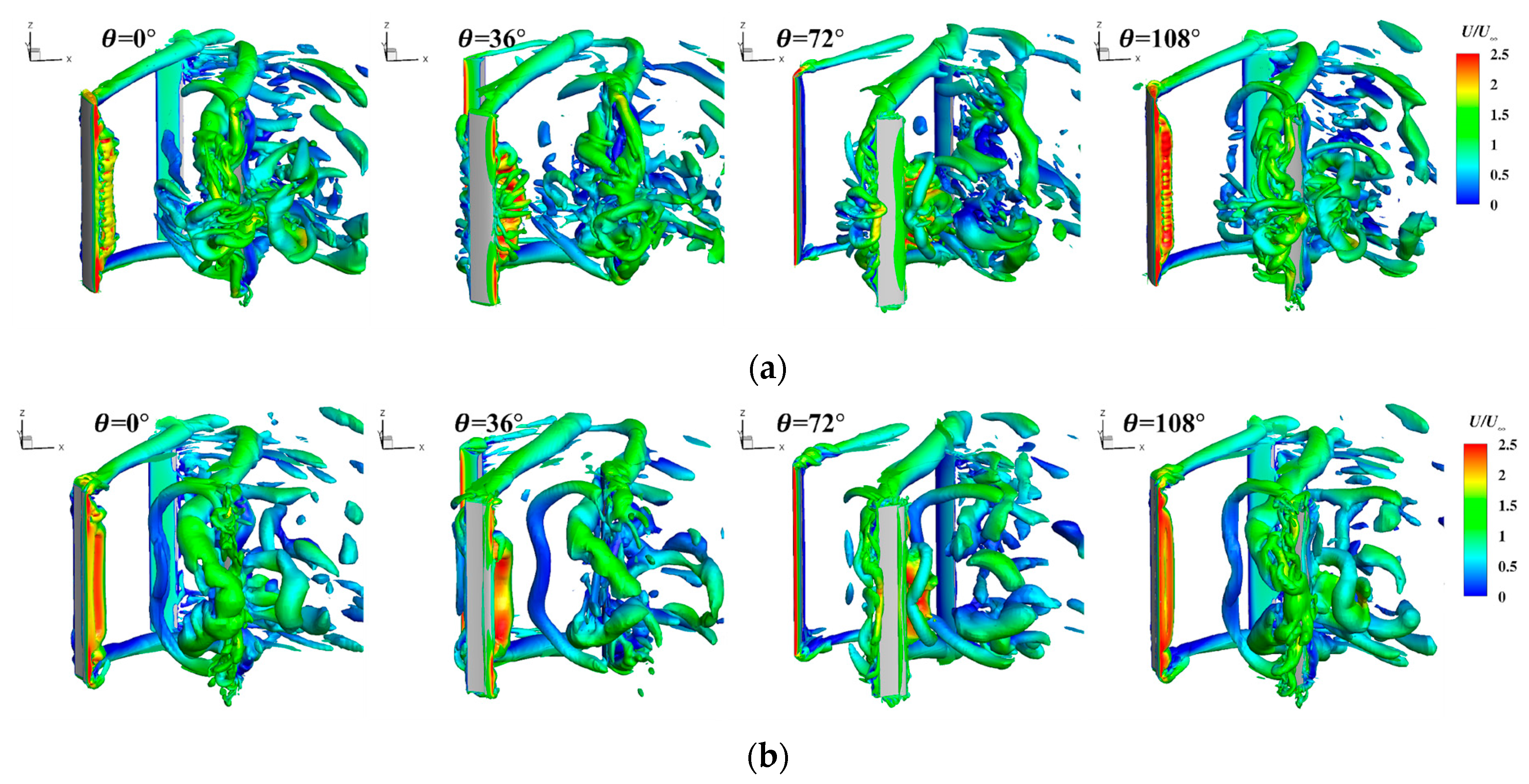
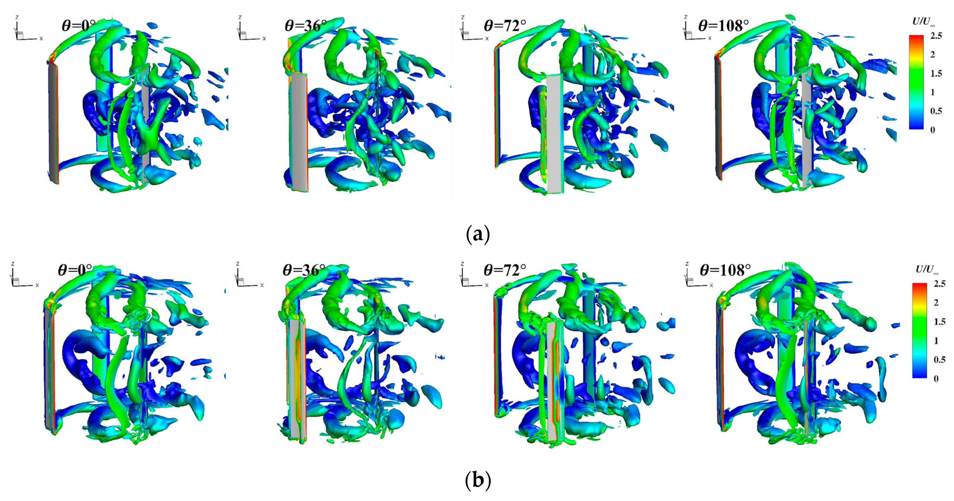
To verify the above conclusions, Figure 20 compares the vortex system evolution of the two types of VAWTs at a low TSR, and it can be observed that when the wind turbine blade started to rotate, the vortex system around the blade was dominated by the tip vortex and is gradually strengthened. With the increase in the angle of attack, the flow separation of the suction surface of the blade starts to occur, and the dynamic stall vortex was formed and gradually strengthened. However, because the tip vortex of the J-shaped blade was stronger, it had an inhibiting effect on the generation and development of the dynamic stall vortex. Therefore, the dynamic stall vortex on the blade surface was significantly smaller than that of the S-shaped blade when severe dynamic stall occurred in the J-shaped blade, and the aerodynamic performance of the J-shaped blade was better than that of the S-shaped blade at this time. The tip vortex and dynamic stall vortex were then ejected from the blade surface to form the wake region, which can have a detrimental effect on the blade, resulting in a negative torque in the wake region. The vortices in the wake region of the J-shaped VAWT were smaller than those of the S-shaped VAWT, allowing for the J-shaped blade to recover more quickly from the negative effects of the wake region.

Figure 20.
Comparison of the evolution process of the vortex system around the blades at a low TSR: (a) S-shaped; (b) J-shaped.
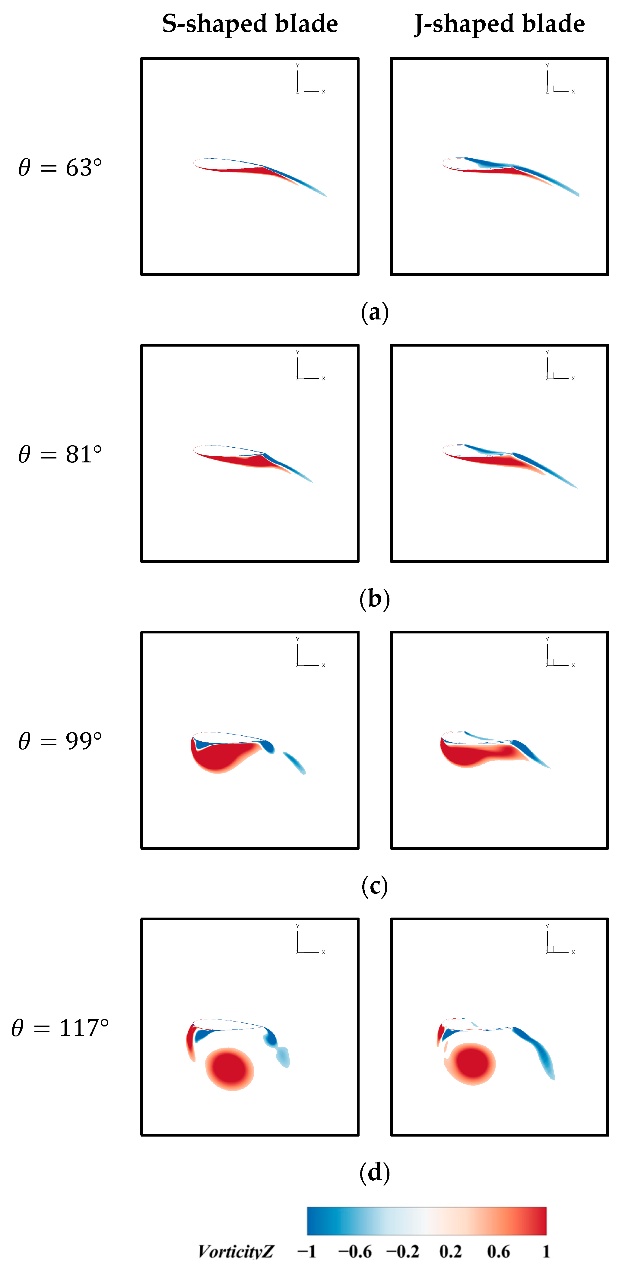
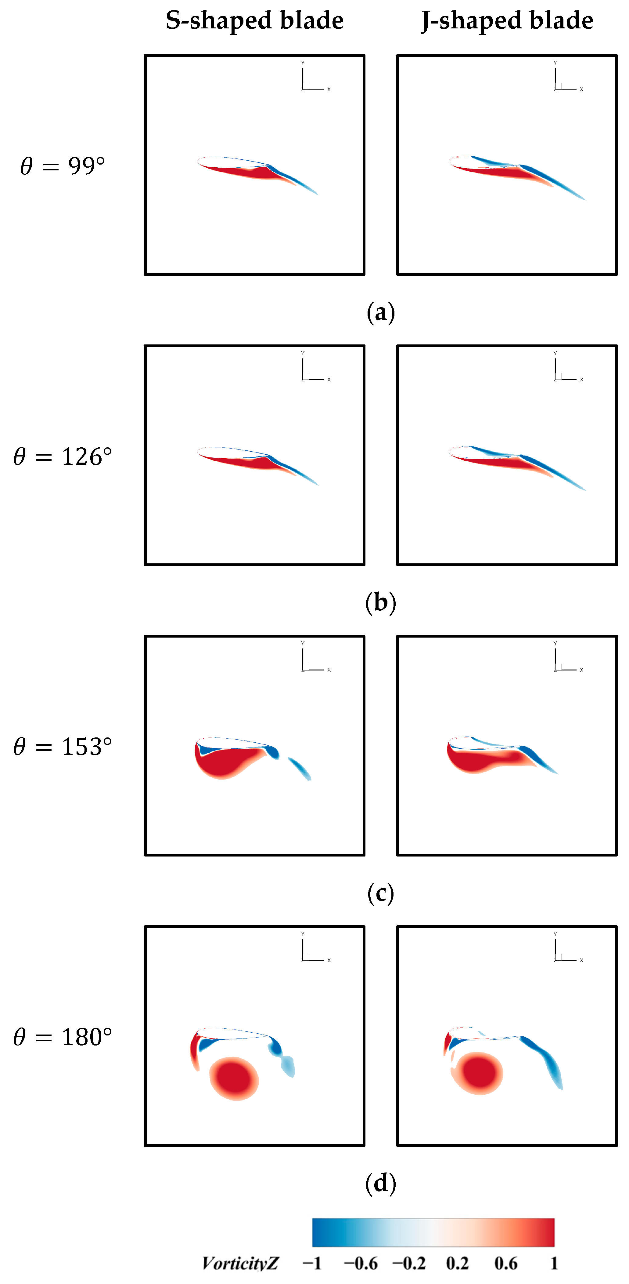
As the J-shape blade can inhibit the generation of the dynamic stall vortex, it has an advantageous range mainly in the area of dynamic stall generation and development. Figure 21 compares the vorticity distributions at the middle section (z = 0) within the dynamic stall vortex development region for two types of blades, and it can be seen that the flow on the suction side of both types of blades is predominantly attached to the blade surface at . However, because the J-shaped blade cuts off a portion of the pressure side, there is a notable disparity in vorticity distribution between the two types of blades on the pressure side. At , significant flow separation was evident in the S-shaped blade, causing the torque coefficient CM to start decreasing. In contrast, only slight flow separation was observed in the J-shaped blade, resulting in a higher CM than the S-shaped blade. Subsequently, the separation point gradually moved forward, the stall vortex intensity gradually increased and finally separated from the leading edge, resulting in a severe dynamic stall. Comparing the vorticity distribution at and , it can be seen that the stall vortex of the J-shaped blade was smaller than that of the S-shaped blade. This indicates that the J-shaped blade has advantages in suppressing flow separation.

Figure 21.
Comparison of vorticity distributions at the middle section around the blades at a low TSR: (a) ; (b) ; (c) ; (d) .
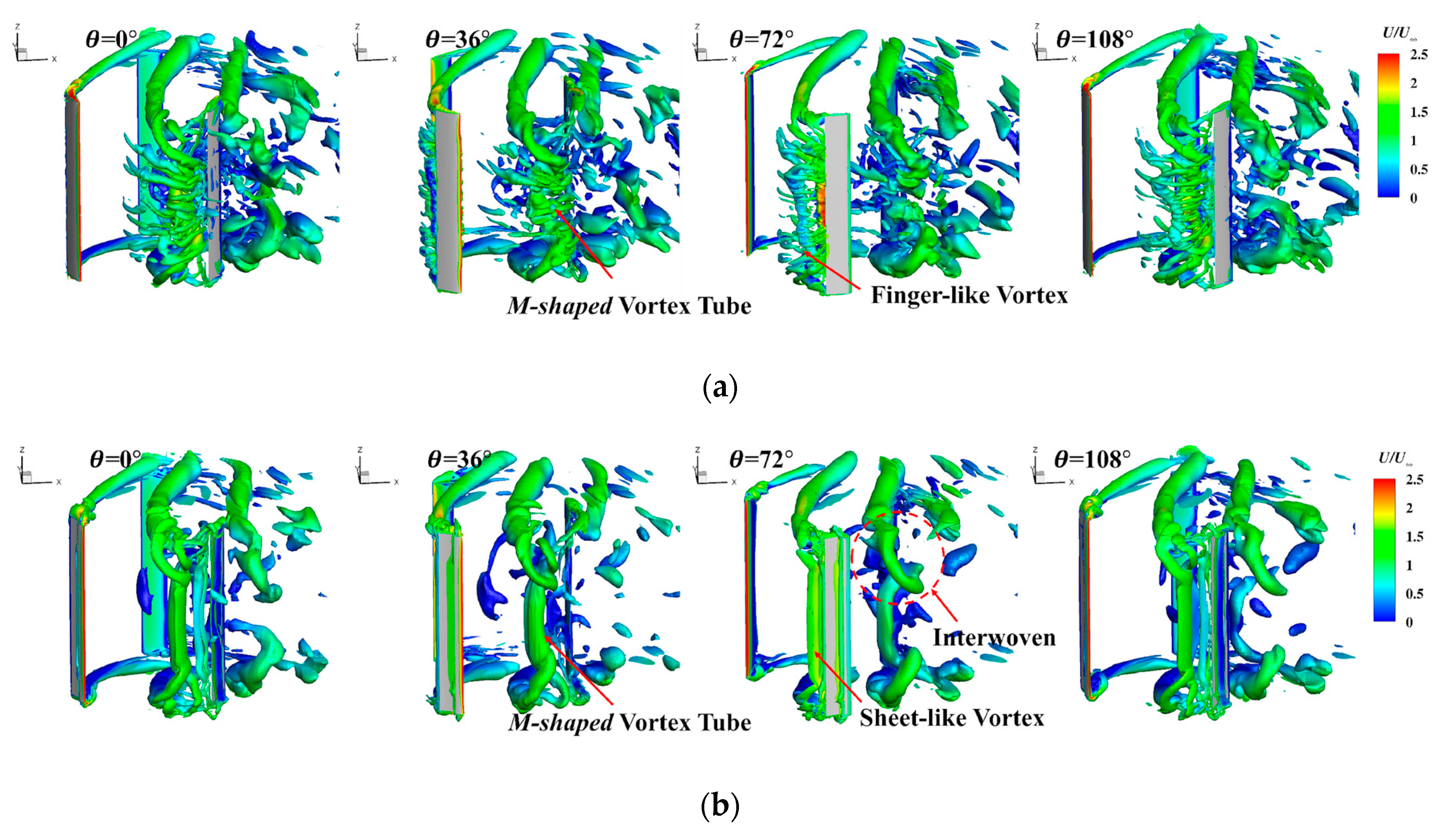
The evolution process of the vortex system in two types of VAWT at a medium TSR is shown in Figure 22. The vortex evolution process was similar to that for a low TSR. Initially, the vortex system was dominated by the tip vortex. With the onset of dynamic stall, a dynamic stall vortex was generated and developed, and finally the vortex detached from the blade surface to form a wake region. Nevertheless, the markedly diminished range of blade angle of attack in comparison to a low TSR served to attenuate the dynamic stall of the blade, while concomitantly reducing the intensity of the dynamic stall vortex. A comparison of the near-field vortex system of the two types of blades reveals that the trailing edge stall vortex of the S-shaped blade exhibits long and numerous finger-like vortexes, whereas the trailing edge stall vortex of the J-shaped blade displays short and diminutive sheet-like vortex. Upon the detachment of the tip vortex and stall vortex, the two vortices coiled around each other and connected to form an M-shaped vortex tube. This M-shaped vortex tube plays a pivotal role in regulating the working environment of the blade in the wake area, which is of paramount importance for the aerodynamic characteristics of the blade in the wake area. It has been demonstrated that the vorticity in the wake region of the J-shaped VAWT was markedly inferior in comparison to that of the S-shaped VAWT.
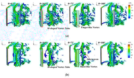
Figure 22.
Comparison of the evolution process of the vortex system around the blades at a medium TSR: (a) S-shaped; (b) J-shaped.
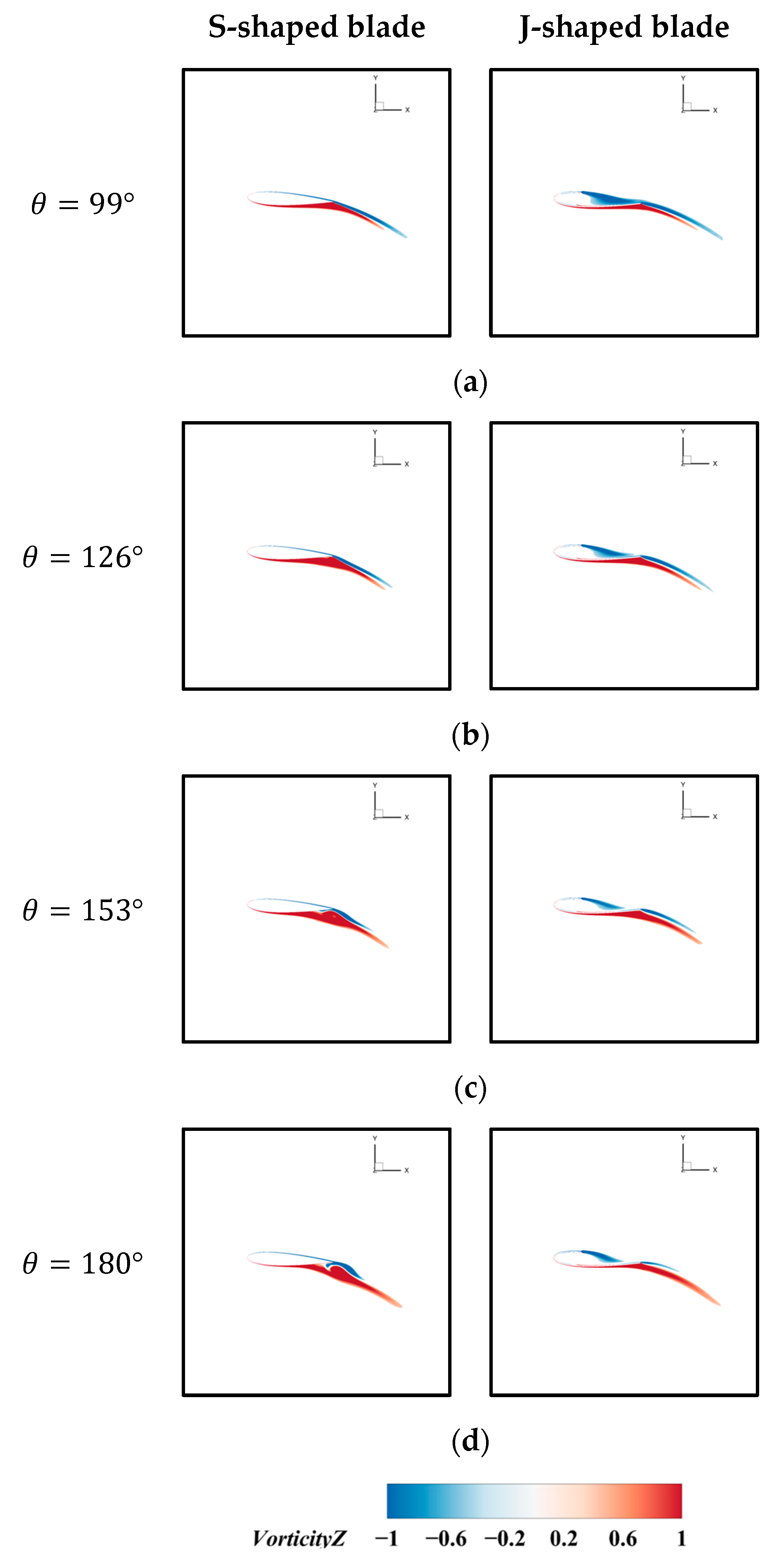
Figure 23 provides a comparison of vorticity distributions at the middle section of the blade for the dynamic stall vortex development process at a medium TSR. It can be clearly observed that the dynamic stall vortex of the J-shaped blade is smaller than that of the S-shaped blade, and the vortex shedding also lags behind that of the S-shaped blade. This explains why the torque coefficient CM of the J-shaped blade is higher than that of the S-shaped blade at these azimuth angles.

Figure 23.
Comparison of vorticity distributions at the middle section around the blades at a medium TSR: (a) ; (b) ; (c) ; (d) .
At a high TSR, the vortex system evolution process of the wind turbine exhibited notable distinctions from that observed at low and medium TSRs. As illustrated in Figure 24, the dynamic stall phenomenon was markedly diminished at a high TSR, the dynamic stall vortex was significantly diminished, and the vortex system was predominantly characterized by the blade tip vortex. This also leads to the conclusion that the J-shaped blade is unable to demonstrate the advantage of suppressing dynamic stall. Figure 25 similarly demonstrates this, showing that within the stall region, the flow around both blade types adheres to the surface without extensive separation, with the J-shaped blades exhibiting no distinct advantages. Furthermore, at the stage when the blade commences its rotational movement, despite the J-shaped blade’s capacity to capture the vortex volume and maintain its containment within the cup profile, the airflow was able to pass through in a smooth and unimpeded manner. This results in an aerodynamic profile that is comparable to that of the S-shaped blade [39]. The aerodynamic characteristics of the J-shaped blade are not as favorable as those of the S-shaped blade at this stage, due to the three dimensional effect and geometric imperfections. Consequently, the CM was lower than that of the S-shaped blade. Meanwhile, the CM of the J-shaped blade in the wake region was lower than that of the S-shaped. The combined J-shaped aerodynamic performance was weaker than the S-shaped in all three regions, so the wind energy utilization of the J-shaped VAWT was much lower than that of the S-shaped VAWT at high tip speeds. However, since most of the VAWTs operate at low to medium tip speed ratios, this does not affect the practical application of the J-shaped VAWT.
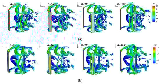
Figure 24.
Comparison of the evolution process of the vortex system around the blades at a high TSR: (a) S-shaped; (b) J-shaped.
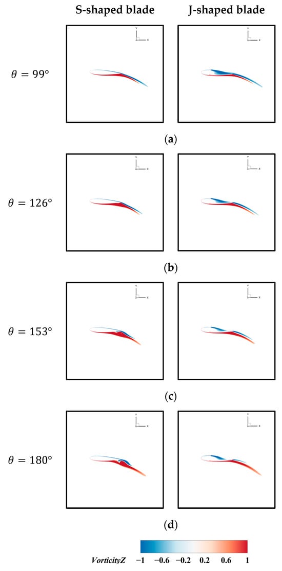
Figure 25.
Comparison of vorticity distributions at the middle section around the blades at a high TSR: (a) ; (b) ; (c) ; (d) .
4. Conclusions
In the current study, the SST-IDDES model was employed to investigate the difference between the aerodynamic performance of S-shaped and J-shaped VAWTs at varying TSRs. The SST-IDDES model is designed to capture complex vortex structures, facilitating a deeper understanding of the J-shaped blade effects on wind turbine aerodynamic performance. The findings reveal that the J-shaped blade demonstrated superior wind energy utilization performance compared to the S-shaped blade at low and medium TSRs. The main conclusions are listed as follows:
- At TSR = 1, the J-shaped blade exhibited a peak CM approximately 13.5% higher and an average CM about 7% higher than the S-shaped blade. The peak CL during dynamic stall was also increased by approximately 11% compared to the S-shaped blade. At TSR = 1.6, the J-shaped blade continued to improve performance, with the peak CM and peak CL increased by 1.8% and 1.5%, respectively, although the improvements were less pronounced than at a lower TSR. Furthermore, the onset of dynamic stall was delayed by approximately 4° to 6° in azimuth for the J-shaped blade under low and medium TSR conditions. These results indicate that the principal positive effect on the enhanced power coefficient of the J-shaped blade is primarily observed in the dynamic stall region. The J-shaped blade exhibited a higher lift coefficient within the stall region, which provides a more substantial positive contribution to the tangential force, enhancing the torque and power coefficients.
- The J-shaped blade exhibited a larger negative pressure zone at the leading edge, increasing the pressure difference between the pressure and suction sides, which boosts the lift coefficient. Moreover, the J-shaped blade had a less pronounced suction zone at the blade tip compared to the S-shaped blade, resulting in a smaller pressure difference between the blade root and tip. Consequently, the cross-flow on the blade surface was weaker, which makes it less prone to flow separation.
- When a wind turbine blade undergoes dynamic stall, the tip vortex interacts with the dynamic stall vortex, forming an -shaped vortex on the blade’s suction side. This -shaped vortex signifies the blade tip vortex’s inhibiting effect on the generation and development of the dynamic stall vortex. Compared to the S-shaped blade, the J-shaped blade generated a stronger tip vortex, which more effectively suppressed the dynamic stall vortex. Consequently, the J-shaped blade exhibited superior performance in suppressing flow separation and delaying dynamic stall.
- After the tip vortex and dynamic stall vortex detached from the blade surface, a wake region was formed, which had a detrimental impact on the wind turbine blades. The wake region vortices of the J-shaped VAWT were significantly fewer than those of the S-shaped VAWT, allowing for the J-shaped blade to recover more quickly from the negative effects of the wake region.
Additionally, this study focused solely on the aerodynamic performance of wind turbines at specific wind speeds and rotational speeds. However, the aerodynamic behavior and vortex evolution process of the J-shaped VAWT under self-starting conditions remain unexplored. Investigating these aspects will be the focus of our future research endeavors.
Author Contributions
Conceptualization, T.Z. and G.W.; methodology, T.Z. and Q.L.; software, G.W. and Q.L.; validation, T.Z.; formal analysis, T.Z.; investigation, T.Z.; resources, G.W.; data curation, T.Z.; writing—original draft preparation, T.Z. and Q.L.; writing—review and editing, G.W.; visualization, Q.L.; supervision, G.W.; project administration, T.Z.; funding acquisition, G.W. All authors have read and agreed to the published version of the manuscript.
Funding
This research was funded by the National Natural Science Foundation of China (no. U2141254 and no. U23B6009).
Data Availability Statement
The data that support the findings of this study are available in this paper.
Acknowledgments
The computations were conducted at the Computing Center in Xi’an. The authors thankfully acknowledge this institution.
Conflicts of Interest
The authors declare no conflicts of interest.
Nomenclature
| Symbols | Abbreviations | ||
| A | swept area of the rotor (m2) | 3D | Three-dimensional |
| c | chord length (m) | CFD | Computational Fluid Dynamics |
| CD | drag coefficient | DDES | Delayed Detached Eddy Simulation |
| CL | lift coefficient | DES | Detached Eddy Simulation |
| CM | torque coefficient | HAWT | Horizontal Axis Wind Turbine |
| CP | power coefficient | IDDES | Improved Delayed Detached Eddy Simulation |
| CT | tangential force coefficient | L.E. | leading edge |
| D | turbine diameter (m) | LES | Large Eddy Simulation |
| M | rotor torque (Nm) | LU-SGS | Lower-Upper Symmetric Gauss-Seidel |
| incoming flow velocity (m/s) | MPI | Message Passing Interface | |
| W | the relative velocity of the blades (m/s) | SST | Shear Stress Transport |
| dimensionless wall distance | T.E. | trailing edge | |
| TSR | Tip Speed Ratio | ||
| Greek | URANS | Unsteady Reynolds Averaged Navier-Stokes | |
| angle of attack () | VAWT | Vertical Axis Wind Turbine | |
| pitch angle () | |||
| azimuthal angle () | |||
| tip speed ratio | |||
| incoming flow density (kg/m3) | |||
| rotational angular velocity (rad/s) | |||
| vorticity (1/s) | |||
| dimensionless vorticity |
References
- Evans, A.; Strezov, V.; Evans, T.J. Assessment of Sustainability Indicators for Renewable Energy Technologies. Renew. Sustain. Energy Rev. 2009, 13, 1082–1088. [Google Scholar] [CrossRef]
- Ismail, M.F.; Vijayaraghavan, K. The Effects of Aerofoil Profile Modification on a Vertical Axis Wind Turbine Performance. Energy 2015, 80, 20–31. [Google Scholar] [CrossRef]
- Rezaeiha, A.; Kalkman, I.; Blocken, B. Effect of Pitch Angle on Power Performance and Aerodynamics of a Vertical Axis Wind Turbine. Appl. Energy 2017, 197, 132–150. [Google Scholar] [CrossRef]
- Buchner, A.-J.; Soria, J.; Honnery, D.; Smits, A.J. Dynamic Stall in Vertical Axis Wind Turbines: Scaling and Topological Considerations. J. Fluid Mech. 2018, 841, 746–766. [Google Scholar] [CrossRef]
- Rolin, V.F.-C.; Porté-Agel, F. Experimental Investigation of Vertical-Axis Wind-Turbine Wakes in Boundary Layer Flow. Renew. Energy 2018, 118, 1–13. [Google Scholar] [CrossRef]
- Kumar, R.; Raahemifar, K.; Fung, A.S. A Critical Review of Vertical Axis Wind Turbines for Urban Applications. Renew. Sustain. Energy Rev. 2018, 89, 281–291. [Google Scholar] [CrossRef]
- Tjiu, W.; Marnoto, T.; Mat, S.; Ruslan, M.H.; Sopian, K. Darrieus Vertical Axis Wind Turbine for Power Generation II: Challenges in HAWT and the Opportunity of Multi-Megawatt Darrieus VAWT Development. Renew. Energy 2015, 75, 560–571. [Google Scholar] [CrossRef]
- Hohman, T.C.; Martinelli, L.; Smits, A.J. The Effects of Inflow Conditions on Vertical Axis Wind Turbine Wake Structure and Performance. J. Wind. Eng. Ind. Aerodyn. 2018, 183, 1–18. [Google Scholar] [CrossRef]
- Hand, B.; Cashman, A. Aerodynamic Modeling Methods for a Large-Scale Vertical Axis Wind Turbine: A Comparative Study. Renew. Energy 2018, 129, 12–31. [Google Scholar] [CrossRef]
- Howell, R.; Qin, N.; Edwards, J.; Durrani, N. Wind Tunnel and Numerical Study of a Small Vertical Axis Wind Turbine. Renew. Energy 2010, 35, 412–422. [Google Scholar] [CrossRef]
- Paraschivoiu, I. Double-Multiple Streamtube Model for Studying Vertical-Axis Wind Turbines. J. Propuls. Power 1988, 4, 370–377. [Google Scholar] [CrossRef]
- Soraghan, C.E.; Leithead, W.E.; Feuchtwang, J.; Yue, H. Double Multiple Streamtube Model for Variable Pitch Vertical Axis Wind Turbines. In Proceedings of the 31st AIAA Applied Aerodynamics Conference, San Diego, CA, USA, 24–27 June 2013; American Institute of Aeronautics and Astronautics: Reston, VA, USA, 2013; p. 2802. [Google Scholar]
- Wang, L.B.; Zhang, L.; Zeng, N.D. A Potential Flow 2-D Vortex Panel Model: Applications to Vertical Axis Straight Blade Tidal Turbine. Energy Convers. Manag. 2007, 48, 454–461. [Google Scholar] [CrossRef]
- Wang, L.; Yeung, R.W. On the Performance of a Micro-Scale Bach-Type Turbine as Predicted by Discrete-Vortex Simulations. Appl. Energy 2016, 183, 823–836. [Google Scholar] [CrossRef]
- Mandal, A.C.; Burton, J.D. The Effects of Dynamic Stall and Flow Curvature on the Aerodynamics of Darrieus Turbines Applying the Cascade Model. Wind Eng. 1994, 18, 267–282. [Google Scholar]
- Le Fouest, S.; Mulleners, K. Optimal Blade Pitch Control for Enhanced Vertical-Axis Wind Turbine Performance. Nat. Commun. 2024, 15, 2770. [Google Scholar] [CrossRef]
- Simão Ferreira, C.; Van Kuik, G.; Van Bussel, G.; Scarano, F. Visualization by PIV of Dynamic Stall on a Vertical Axis Wind Turbine. Exp. Fluids 2009, 46, 97–108. [Google Scholar] [CrossRef]
- Van Der Deijl, W.; Obligado, M.; Sicot, C.; Barre, S. Experimental Study of Mean and Turbulent Velocity Fields in the Wake of a Twin-Rotor Vertical Axis Wind Turbine. J. Phys. Conf. Ser. 2022, 2265, 22073. [Google Scholar] [CrossRef]
- Buchner, A.-J.; Lohry, M.W.; Martinelli, L.; Soria, J.; Smits, A.J. Dynamic Stall in Vertical Axis Wind Turbines: Comparing Experiments and Computations. J. Wind. Eng. Ind. Aerodyn. 2015, 146, 163–171. [Google Scholar] [CrossRef]
- Barnes, A.; Marshall-Cross, D.; Hughes, B.R. Towards a Standard Approach for Future Vertical Axis Wind Turbine Aerodynamics Research and Development. Renew. Sustain. Energy Rev. 2021, 148, 111221. [Google Scholar] [CrossRef]
- Spalart, P.; Jou, W.-H.; Strelets, M.; Allmaras, S. Comments on the Feasibility of LES for Wings, and on a Hybrid RANS/LES Approach. In Proceedings of the First AFOSR International Conference on DNS/LES, Ruston, LA, USA, 4–8 August 1997; Greyden Press: Columbus, OH, USA, 1997; pp. 137–147. [Google Scholar]
- Spalart, P.R.; Deck, S.; Shur, M.L.; Squires, K.D.; Strelets, M.K.; Travin, A. A New Version of Detached-Eddy Simulation, Resistant to Ambiguous Grid Densities. Theoret. Comput. Fluid Dyn. 2006, 20, 181–195. [Google Scholar] [CrossRef]
- Shur, M.L.; Spalart, P.R.; Strelets, M.K.; Travin, A.K. A Hybrid RANS-LES Approach with Delayed-DES and Wall-Modelled LES Capabilities. Int. J. Heat Fluid Flow 2008, 29, 1638–1649. [Google Scholar] [CrossRef]
- Lei, H.; Zhou, D.; Bao, Y.; Li, Y.; Han, Z. Three-Dimensional Improved Delayed Detached Eddy Simulation of a Two-Bladed Vertical Axis Wind Turbine. Energy Convers. Manag. 2017, 133, 235–248. [Google Scholar] [CrossRef]
- Chen, J.; Chen, L.; Xu, H.; Yang, H.; Ye, C.; Liu, D. Performance Improvement of a Vertical Axis Wind Turbine by Comprehensive Assessment of an Airfoil Family. Energy 2016, 114, 318–331. [Google Scholar] [CrossRef]
- Huang, H.; Luo, J.; Li, G. Study on the Optimal Design of Vertical Axis Wind Turbine with Novel Variable Solidity Type for Self-Starting Capability and Aerodynamic Performance. Energy 2023, 271, 127031. [Google Scholar] [CrossRef]
- Ardaneh, F.; Abdolahifar, A.; Karimian, S.M.H. Numerical Analysis of the Pitch Angle Effect on the Performance Improvement and Flow Characteristics of the 3-PB Darrieus Vertical Axis Wind Turbine. Energy 2022, 239, 122339. [Google Scholar] [CrossRef]
- Singh, E.; Roy, S.; Yam, K.S.; Law, M.C. Numerical Analysis of H-Darrieus Vertical Axis Wind Turbines with Varying Aspect Ratios for Exhaust Energy Extractions. Energy 2023, 277, 127739. [Google Scholar] [CrossRef]
- Zhu, C.; Yang, H.; Qiu, Y.; Zhou, G.; Wang, L.; Feng, Y.; Shen, Z.; Shen, X.; Feng, X.; Wang, T. Effects of the Reynolds Number and Reduced Frequency on the Aerodynamic Performance and Dynamic Stall Behaviors of a Vertical Axis Wind Turbine. Energy Convers. Manag. 2023, 293, 117513. [Google Scholar] [CrossRef]
- Peng, H.Y.; Lam, H.F. Turbulence Effects on the Wake Characteristics and Aerodynamic Performance of a Straight-Bladed Vertical Axis Wind Turbine by Wind Tunnel Tests and Large Eddy Simulations. Energy 2016, 109, 557–568. [Google Scholar] [CrossRef]
- Xu, W.; Li, C.; Huang, S.; Wang, Y. Aerodynamic Performance Improvement Analysis of Savonius Vertical Axis Wind Turbine Utilizing Plasma Excitation Flow Control. Energy 2022, 239, 122133. [Google Scholar] [CrossRef]
- Shukla, V.; Kaviti, A.K. Performance Evaluation of Profile Modifications on Straight-Bladed Vertical Axis Wind Turbine by Energy and Spalart Allmaras Models. Energy 2017, 126, 766–795. [Google Scholar] [CrossRef]
- Ghafoorian, F.; Enayati, E.; Mirmotahari, S.R.; Wan, H. Self-Starting Improvement and Performance Enhancement in Darrieus VAWTs Using Auxiliary Blades and Deflectors. Machines 2024, 12, 806. [Google Scholar] [CrossRef]
- Attie, C.; ElCheikh, A.; Nader, J.; Elkhoury, M. Performance Enhancement of a Vertical Axis Wind Turbine Using a Slotted Deflective Flap at the Trailing Edge. Energy Convers. Manag. 2022, 273, 116388. [Google Scholar] [CrossRef]
- MacPhee, D.; Beyene, A. Recent Advances in Rotor Design of Vertical Axis Wind Turbines. Wind. Eng. 2012, 36, 647–665. [Google Scholar] [CrossRef]
- Bhuyan, S.; Biswas, A. Investigations on Self-Starting and Performance Characteristics of Simple H and Hybrid H-Savonius Vertical Axis Wind Rotors. Energy Convers. Manag. 2014, 87, 859–867. [Google Scholar] [CrossRef]
- Wakui, T.; Tanzawa, Y.; Hashizume, T.; Nagao, T. Hybrid Configuration of Darrieus and Savonius Rotors for Stand-Alone Wind Turbine-Generator Systems. Electr. Eng. Jpn. 2005, 150, 13–22. [Google Scholar] [CrossRef]
- Ghafoorian, F.; Hosseini Rad, S.; Moghimi, M. Enhancing Self-Starting Capability and Efficiency of Hybrid Darrieus–Savonius Vertical Axis Wind Turbines with a Dual-Shaft Configuration. Machines 2025, 13, 87. [Google Scholar] [CrossRef]
- Zamani, M.; Maghrebi, M.J.; Varedi, S.R. Starting Torque Improvement Using J-Shaped Straight-Bladed Darrieus Vertical Axis Wind Turbine by Means of Numerical Simulation. Renew. Energy 2016, 95, 109–126. [Google Scholar] [CrossRef]
- Zamani, M.; Nazari, S.; Moshizi, S.A.; Maghrebi, M.J. Three Dimensional Simulation of J-Shaped Darrieus Vertical Axis Wind Turbine. Energy 2016, 116, 1243–1255. [Google Scholar] [CrossRef]
- Mohamed, M.H. Criticism Study of J-Shaped Darrieus Wind Turbine: Performance Evaluation and Noise Generation Assessment. Energy 2019, 177, 367–385. [Google Scholar] [CrossRef]
- Pan, L.; Zhu, Z.; Xiao, H.; Wang, L. Numerical Analysis and Parameter Optimization of J-Shaped Blade on Offshore Vertical Axis Wind Turbine. Energies 2021, 14, 6426. [Google Scholar] [CrossRef]
- García Auyanet, A.; Santoso, R.E.; Mohan, H.; Rathore, S.S.; Chakraborty, D.; Verdin, P.G. CFD-Based J-Shaped Blade Design Improvement for Vertical Axis Wind Turbines. Sustainability 2022, 14, 15343. [Google Scholar] [CrossRef]
- Celik, Y.; Ingham, D.; Ma, L.; Pourkashanian, M. Design and Aerodynamic Performance Analyses of the Self-Starting H-Type VAWT Having J-Shaped Aerofoils Considering Various Design Parameters Using CFD. Energy 2022, 251, 123881. [Google Scholar] [CrossRef]
- Farzadi, R.; Bazargan, M. 3D Numerical Simulation of the Darrieus Vertical Axis Wind Turbine with J-Type and Straight Blades under Various Operating Conditions Including Self-Starting Mode. Energy 2023, 278, 128040. [Google Scholar] [CrossRef]
- Li, Q.; Sun, X.; Wang, G. Detached-Eddy Simulation of the Vortex System on the High-Lift Common Research Model. Phys. Fluids 2024, 36, 025173. [Google Scholar] [CrossRef]
- Wang, G.; Li, Q.; Liu, Y. IDDES Method Based on Differential Reynolds-Stress Model and Its Application in Bluff Body Turbulent Flows. Aerosp. Sci. Technol. 2021, 119, 107207. [Google Scholar] [CrossRef]
- Li, Q.; Chen, X.; Wang, G.; Liu, Y. A Dynamic Version of the Improved Delayed Detached-Eddy Simulation Based on the Differential Reynolds-Stress Model. Phys. Fluids 2022, 34, 115112. [Google Scholar] [CrossRef]
- Chen, X.; Wang, G.; Ye, Z. Wind Tunnel Wall Interference Correction for Transonic Airfoils with Data-Reduced Ensemble Kalman Filter. Phys. Fluids 2024, 36, 105139. [Google Scholar] [CrossRef]
- Wang, G.; Chen, X.; Xing, Y.; Zeng, Z. Multi-Body Separation Simulation with an Improved General Mesh Deformation Method. Aerosp. Sci. Technol. 2017, 71, 763–771. [Google Scholar] [CrossRef]
- Zhou, H.; Nie, M.; Qin, M.; Wang, G. An Unsteady Aerodynamic Reduced-Order Modelling Framework for Shock-Dominated Flow with Application on Shock-Induced Panel Flutter Prediction. J. Fluids Struct. 2025, 133, 104251. [Google Scholar] [CrossRef]
- Wang, G.; Ye, Z.-Y. Mixed Element Type Unstructured Grid Generation and Its Application to Viscous Flow Simulation. In Proceedings of the 24th International Congress of Aeronautical Sciences, Yokohama, Japan, 29 August–3 September 2004; p. 2004-2. [Google Scholar]
- Menter, F.R. Two-Equation Eddy-Viscosity Turbulence Models for Engineering Applications. AIAA J. 1994, 32, 1598–1605. [Google Scholar] [CrossRef]
- Ferreira, C.S.; Geurts, B. Aerofoil Optimization for Vertical-Axis Wind Turbines. Wind Energy 2015, 18, 1371–1385. [Google Scholar] [CrossRef]
- Lei, H.; Su, J.; Bao, Y.; Chen, Y.; Han, Z.; Zhou, D. Investigation of Wake Characteristics for the Offshore Floating Vertical Axis Wind Turbines in Pitch and Surge Motions of Platforms. Energy 2019, 166, 471–489. [Google Scholar] [CrossRef]
- Lam, H.F.; Peng, H.Y. Study of Wake Characteristics of a Vertical Axis Wind Turbine by Two- and Three-Dimensional Computational Fluid Dynamics Simulations. Renew. Energy 2016, 90, 386–398. [Google Scholar] [CrossRef]
- Dessoky, A.; Lutz, T.; Bangga, G.; Krämer, E. Computational Studies on Darrieus VAWT Noise Mechanisms Employing a High Order DDES Model. Renew. Energy 2019, 143, 404–425. [Google Scholar] [CrossRef]
- Bravo, R.; Tullis, S.; Ziada, S. Performance Testing of a Small Vertical-Axis Wind Turbine. In Proceedings of the 21st Canadian Congress of Applied Mechanics, Toronto, ON, Canada, 3–7 June 2007; pp. 470–471. [Google Scholar]
- Daróczy, L.; Janiga, G.; Petrasch, K.; Webner, M.; Thévenin, D. Comparative Analysis of Turbulence Models for the Aerodynamic Simulation of H-Darrieus Rotors. Energy 2015, 90, 680–690. [Google Scholar] [CrossRef]
- Su, J.; Chen, Y.; Han, Z.; Zhou, D.; Bao, Y.; Zhao, Y. Investigation of V-Shaped Blade for the Performance Improvement of Vertical Axis Wind Turbines. Appl. Energy 2020, 260, 114326. [Google Scholar] [CrossRef]
- Narayan, G.; John, B. Effect of Winglets Induced Tip Vortex Structure on the Performance of Subsonic Wings. Aerosp. Sci. Technol. 2016, 58, 328–340. [Google Scholar] [CrossRef]
- Liu, C.; Gao, Y.; Tian, S.; Dong, X. Rortex—A New Vortex Vector Definition and Vorticity Tensor and Vector Decompositions. Phys. Fluids 2018, 30, 035103. [Google Scholar] [CrossRef]
- Spentzos, A.; Barakos, G.N.; Badcock, K.J.; Richards, B.E.; Coton, F.N.; Galbraith, R.A. McD.; Berton, E.; Favier, D. Computational Fluid Dynamics Study of Three-Dimensional Dynamic Stall of Various Planform Shapes. J. Aircr. 2007, 44, 1118–1128. [Google Scholar] [CrossRef]
- Xu, W.; Li, G.; Wang, F.; Li, Y. High-Resolution Numerical Investigation into the Effects of Winglet on the Aerodynamic Performance for a Three-Dimensional Vertical Axis Wind Turbine. Energy Convers. Manag. 2020, 205, 112333. [Google Scholar] [CrossRef]


Disclaimer/Publisher’s Note: The statements, opinions and data contained in all publications are solely those of the individual author(s) and contributor(s) and not of MDPI and/or the editor(s). MDPI and/or the editor(s) disclaim responsibility for any injury to people or property resulting from any ideas, methods, instructions or products referred to in the content. |
© 2025 by the authors. Licensee MDPI, Basel, Switzerland. This article is an open access article distributed under the terms and conditions of the Creative Commons Attribution (CC BY) license (https://creativecommons.org/licenses/by/4.0/).