Article

Active Vibration Control of Cantilever Structures by Integrating the Closed Loop Control Action into Transient Solution of Finite Element Model and an Application to Aircraft Wing

1
Department of Mechanical Engineering, Dokuz Eylul University, Buca 35390, Türkiye
2
Department of Mechatronics Engineering, Izmir University of Economics, İzmir 35330, Türkiye
*
Author to whom correspondence should be addressed.
Machines 2025, 13(5), 379; https://doi.org/10.3390/machines13050379
Submission received: 3 March 2025 / Revised: 24 April 2025 / Accepted: 27 April 2025 / Published: 30 April 2025
(This article belongs to the Special Issue Active Vibration Control System)

Abstract

:
In this study, the active vibration control (AVC) of a cantilever beam with an end mass is considered first and studied experimentally and through simulation. The Laplace transform method, Newmark method, and ANSYS are used for simulations. An impulse force applied to the mass and the velocity actuation applied to the base are assumed to be disturbance and controlling input, respectively. The displacement of the mass is taken as the feedback signal in simulations. Four strain gauges are located near the bottom point, connected with a Wheatstone bridge, and the output voltage of a load-cell amplifier (LCA) is used as the feedback signal in experiments. Strain feedback is considered in experiments because it is easy to implement, cost-effective, and can be used in applications. Experimental displacement signals obtained from the top of the beam are compared with the output signals from LCA and it is observed that they are approximately linearly dependent. Velocity input is generated with a servo motor-driven linear actuator in experiments. The closed loop control is achieved by a personal computer with an Adlink-9222 PCI DAQ card and a C program in the experiments. The integration of the closed loop control action into the transient solution with Newmark method and ANSYS is implemented in simulations. The input reference value is taken as zero for vibration control. The instantaneous value of the feedback signal at a time step is subtracted from zero to find the error signal value and the error value is multiplied by the control gain to calculate the controlling signal. The simulation results obtained with the Newmark method and ANSYS are in good agreement with the analytical results obtained with Laplace transform method. Simulation results are also in acceptable agreement with the experimental results for explaining the behavior of the success of AVC depending on the control gain, Kp. After verifying ANSYS solutions, the ANSYS procedure is applied to an aircraft wing as a real complex cantilever structure. The wing, with a length of 810.8 mm, 13 ribs with a length of 300 mm, and NACA 4412 airfoil, is considered in this study. It is observed that the AVC of real engineering structures can be simulated by integrating control action into transient solution in ANSYS.

1. Introduction

Flexible cantilever structures are widely used in engineering applications such as civil engineering structures, construction machines, robot manipulators, aircraft wings, satellite antennas, solar panels, and marine risers. Flexible structures undergo higher vibrations and thus vibration control has attracted the attention of many researchers [1]. Wang et al. [1] studied a cantilever beam with end mass and designed an adaptive boundary controller to suppress vibration. They used a partial differential equation of the beam. Lyu et al. [2] proposed a vibration control method for cantilever beams which uses a combined macro-fiber composite (MFC) and rotary motor actuators. They modeled the system using Euler–Bernoulli beam theory, used orthogonal polynomials as mode shapes and obtained superior vibration control with combined actuation as compared with using actuators alone. Li et al. [3] used a hybrid PID-FxLMS algorithm for active vibration control (AVC) of a cantilever beam with a piezoelectric stack actuator. They modeled the system in ABAQUS to obtain a state space model for simulation and verified the simulation results with experiments. They observed that the vibration suppression performance of the hybrid control was much better than that of the FxLMS algorithm or traditional PID controller alone. Amer et al. [4] considered the linear velocity feedback control, the cubic velocity feedback control, the non-linear saturation controller, and the positive position feedback (PPF) controllers and they observed that the PPF controller was the best controller for the AVC of cantilever beams. Saif et al. [5] explored the direct application of a deep learning technique and an approach which integrated deep learning into a PID controller for AVC of cantilever beams. They compared the two techniques to evaluate effectiveness and strengths and offered their potential applications. Huang et al. [6] studied the AVC of composite cantilever beams with the finite element (FE) method and Golla–Hughes–McTavish model. They optimized the linear quadratic feedback gain using particle swarm optimization. Djokoto et al. [7] studied a micro-cantilever beam (MCB) with electrorheological fluid (ERF) support. They presented results showing the vibration controlling of MCB by activating ERF with an electric field. Cui et al. [8] proposed a finite element model of a piezoelectric cantilever beam using the Hamilton variation principle. They employed the independent modal space method based on a linear quadratic regulator and verified the effectiveness of the proposed model and AVC with numerical solutions and experiments. Umar et al. [9] employed integrating a non-symmetric Bouc–Wen model with an auto-regressive model with eXogenous inputs to enhance the AVC of a cantilever beam using MFC. Their approach showed potential for practical engineering applications. Teoh et al. [10] used the receptance method for the robust control of DigiTwin Operating Platform. They proposed an algorithm which involves estimating the transfer function approximately by a rational fraction polynomial curve fitting method from the frequency response function matrix found experimentally, and then obtained the control gains. Karagülle et al. [11] realized the integration of the control action into ANSYS solution for the AVC of a cantilever beam with piezoelectric actuation.
There are studies on AVC of cantilever structures in civil engineering and aerospace. Ito et al. [12] proposed using cameras and image processing for the displacement for feedback measurements for AVC in the low frequency band (0–1.5 Hz), which is applicable in high-rise buildings. Ramírez-Neria et al. [13] presented active disturbance rejection control for seismically excited building structures. They used a five-story building structure, an active mass damper as the controlling actuator, and a shaking table as the disturbance. Gehni et al. [14] explored deep reinforcement learning (DRL) for controlling vibrations in building structures. They proposed a DRL-based control framework that learns to adjust the control signal using adaptive linear quadratic regulator.
Zhang et al. [15] presented an approach to mitigate vibrations induced by external shock on composite structures, which are used in the fuselage of airplanes. They used a deep learning network to enhance control efficiency. He et al. [16] studied the AVC of a blended-wing-body airplane wing by using a smooth-switching linear-parameter-varying dynamic output–feedback control. Li et al. [17] proposed an improved parallel multi-input, multi-output, multi-frequency filtered-x least mean square control algorithm for the AVC of an aircraft panel structure using piezoelectric stack actuators. Dong et al. [18] presented phase compensation active disturbance rejection control for shimmy vibration using a magnetorheological damper. Sahin et al. [19] studied smart beam and fin structures with bonded piezoelectric patches to suppress free and forced vibrations using H∞ and sliding mode controllers. They presented simulation and experimental results. Prakash et al. [20] designed a field programmable gate array-based multi-channel feedforward adaptive filtered-x least mean square algorithm-based AVC. They deployed the developed system for AVC testing of the full-scale wing of a composite two-seater transport aircraft and obtained encouraging results.
In this study, we aimed to study the AVC of cantilever structures with ANSYS (APDL 2021 R1). Commercial computer-aided engineering (CAE) programs are widely used in the simulation age with computers for analyzing real complex engineering systems. The user defines the system and inputs only, and the CAE software develop a mathematical model and give the solutions for static, harmonic, and transient analyses. There is no direct modeling and solutions for closed loop control systems in ANSYS. A procedure which integrates control action into the transient solution in ANSYS APDL is given in this study. The validity of the procedure is tested by comparing the results with the solutions obtained with the Laplace transform and Newmark methods for a cantilever beam with an end mass. Experimental results are also given. Then, the procedure is used for the AVC of an aircraft wing.
This paper consists of the following sections. Simulations of the AVC of a cantilever beam with end mass with FE modeling, Laplace transform method, Newmark method, and ANSYS APDL are given in Section 2. The experimental system is described in Section 3. Simulation of AVC of an aircraft wing using ANSYS APDL is explained in Section 4. The results and discussion are presented in Section 5. Finally, the conclusions of the study are given in Section 6.

2. Simulation of Active Vibration Control of Cantilever Beam with End Mass

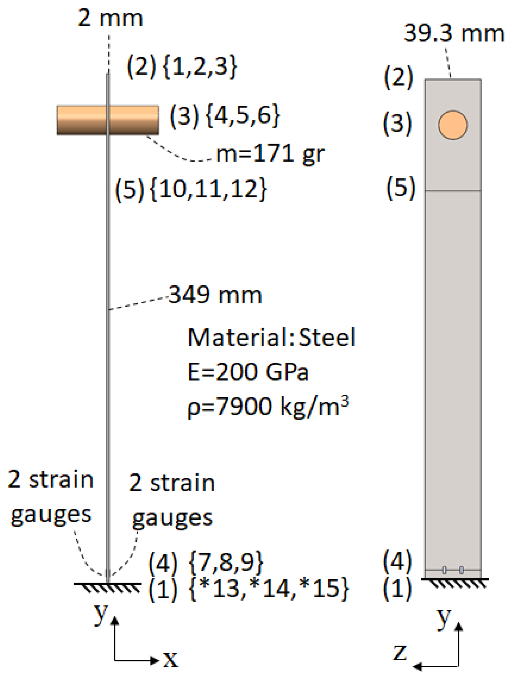
2.1. Finite Element Model for Laplace Transform and Newmark Method Solution

The mathematical model of the system under study is developed for the analysis with the Laplace Transform and Newmark methods. The cantilever beam considered is shown in Figure 1.
The nodes are numbered in round brackets as (1) to (5). The FE assembly is defined in Table 1.
The local origin is at Node-4 and the end point is at Node-5; the local x axis, x2, is in the direction from Node-4 to Node-5; the length is 265 mm; the orientation angle is 90° for FE-2 for example. The nodal displacement indices of the assembled system in global coordinates are shown in curly brackets in Figure 1. For example, the indices for Node-5, {10,11,12}, correspond to [d10, d11, d12]’, where d10, d11, and d12 are the displacement in the x direction, the displacement in the y direction, and the bending rotation of the cross-section about z axis at Node-5, respectively. The prime symbol indicates the transpose of the matrix. The known nodal displacements are numbered at last following the symbol asterisk (*). For FE-2, the displacement vector with the indices for the assembled system is [d7, d8, d9, d10, d11, d12]’.
The end mass is located at Node-3. The degree of freedom of the system, ndof, is 12. The impulse force, fd, applied in the x direction at Node-3 (in the direction of d4) is considered as the disturbance. The feedback signal in AVC, dm, is considered as the displacement in the x direction of the end mass. Thus, dm = d4. The effect of the impulse disturbance is high if it is applied towards the free end of the beam. The displacement feedback signal is also high if it is taken towards the end of the free end of the beam. Thus, Node-3 is selected for the impulse disturbance and the displacement feedback. The active vibration controlling velocity actuation, vs, is applied to the support in the x direction at Node-1. Thus, vs = d ˙ s = d ˙ 13.
Each finite element (FE) has stiffness and mass matrices in local coordinates as [KFE-L]n, and [MFE-L]n, respectively. Here, n is the index of FE. The FE stiffness and mass matrices in local coordinates for the Bernoulli–Euler beam are given below [21].
K F E _ L = A E h 0 0 A E h 0 0 0 12 E I h 3 6 E I h 2 0 12 E I h 3 6 E I h 2 0 6 E I h 2 4 E I h 0 6 E I h 2 2 E I h A E h 0 0 A E h 0 0 0 12 E I h 3 6 E I h 2 0 12 E I h 3 6 E I h 2 0 6 E I h 2 2 E I h 0 6 E I h 2 4 E I h     M F E L = ρ A h 420 140 0 0 70 0 0 0 156 22 h 0 54 13 h 0 22 h 4 h 2 0 13 h 3 h 2 70 0 0 140 0 0 0 54 13 h 0 156 22 h 0 13 h 3 h 2 0 22 h 4 h 2
Here E, ρ, h, A, and I are the elasticity modulus, density, the length, cross-sectional area, and bending moment of inertia of the cross-section. The transformed FE stiffness and mass matrices in global coordinates of FE-n are [KFE]n, and [MFE]n, can be found from the following Equations [21]:
[KFE] = [TFE]’[KFE-L][TFE], [MFE] = [TFE]’[MFE-L][TFE]
where the transformation matrix is given as:
T F E = c s 0 0 0 0 s c 0 0 0 0 0 0 1 0 0 0 0 0 0 c s 0 0 0 0 s c 0 0 0 0 0 0 1
Here, φ is the orientation angle of the FE, and c = cosφ, s = sinφ.
The mathematical model of the system can be written as [M]{ d ¨ } + [C]{ d ˙ } + [K]{d} = {f}, where [M], [C], and [K] are mass, damping, and stiffness matrices of the system having a size of (15 × 15); {d} is the displacement vector of the system with 15 rows; and {f} is the nodal forces vector of the system with 15 rows. The assembled system matrices can be obtained using Table 1. For example, the 9th row and 7th column of [M] matrix is found by considering that the combinations of these global displacement indices are available in FE-1 and FE-2 as given in Table 1. These global indices correspond to 6th row and 4th column of [MFE] of FE-1 and 3rd row 1st column of [MFE] of FE-2. Then, the 9th row and 7th column of [M] = 6th row and 4th column of [MFE] of FE-1 + 3rd row and 1st column of [MFE] of FE-2.
For example, the 10th row and 10th column of [K] matrix is found by considering that the combinations of these global displacement indices are available in FE-2 and FE-3 as given in Table 1. These global indices correspond to 4th row and 4th column of [KFE] of FE-2 and 1st row and 1st column of [KFE] of FE-3. Then, the 10th row and 10th column of [K] = 4th row and 4th column of [KFE] of FE-2 + 1st row and 1st column of [KFE] of FE-3.
All the elements of [M] and [K] matrices are found using the algorithm explained in the examples above.
The damping matrix of the system can be written as [C] = α[M] + β[K], where α and β are Rayleigh damping coefficients [21].
The system displacement vector can be written as:
{d} = [d1, d2, d3, d4, d5, d6, d7, d8, d9, d10, d11, d12, d13, 0, 0]’
Here, d13 = 0 for without AVC (Control-Off case). d ˙ 13 = d ˙ s = vs is the controlling input for AVC (Control-On case).
The system nodal force vector can be written as:
{f} = [0, 0, 0, fd, 0, 0, 0, 0, 0, 0, 0, 0, FAx, FAy, MA]’
where FAx, FAy, and MA are the reaction forces at the Node-1.
The mass matrix of the system, [M], is sub-divided into four matrices; [Ma], [Mb], [Mc], and [Md]. [Ma] is obtained by taking 1–12 rows, and 1–12 columns of [M]. [Mb] is obtained by taking 1–12 rows, and 13–15 columns of [M]. [Mc] is obtained by taking 13–15 rows, and 1–12 columns of [M]. [Md] is obtained by taking 13–15 rows, and 13–15 columns of [M]. [Ka], [Kb], [Kc], [Kd], [Ca], [Cb], [Cc], [Cd] matrices are obtained similarly.
The assembled system displacement vector is sub-divided to two vectors as:
{da} = [d1, d2, d3, d4, d5, d6, d7, d8, d9, d10, d11, d12]’ and {db} = [d13, 0,0]’
The assembled system nodal force vector is sub-divided to two vectors as:
{fa} = [0, 0, 0, fd, 0, 0, 0, 0, 0, 0, 0, 0]’ and {fb} = [FAx, FAy, MA]’
Here {db} and {fa} are time-dependent inputs, and {da} and {fb} are to be calculated as outputs.
The following equations can be written:
[ M a ] { d ¨ a } + [ C a ] { d ˙ a } + [ K a ] { d a } = { f a } [ M b ] { d ¨ b } [ C b ] { d ˙ b } [ K b ] { d b }
{ f b } = [ M c ] { d ¨ a } + [ C c ] { d ˙ a } + [ K c ] { d a } + [ M d ] { d ¨ b } + [ C d ] { d ˙ b } + [ K b ] { d b }
Equation (4) is the mathematical FE model of the system, which is a set of linear differential equations and can be solved analytically by the Laplace transform method, or by numerical methods like the Newmark method [21]. Equation (4) is solved to find {da}, and then Equation (5) is solved to find {fb].
A MatLAB program is developed to obtain [Ma], [Mb], [Mc], [Md], [Ca], [Cb], [Cc], [Cd], [Ka], [Kb], [Kc], [Kd] from the inputs in Table 1, E, ρ, I, A. (MatLAB: R2024a)

2.2. Simulation by Laplace Transform Method

The following equation can be found by taking the Laplace transform of Equation (4) [22]:
{Da} = [Ho]{Fa} − [Ho][s2[Mb] + s[Cb] + [Kb]]{Db}
where
[Ho] = [s2[Ma] + s[Ca] + [Ka]]−1
Here, {Da}, {Fa}, and {Db} are the Laplace transforms of {da}, {fa}, and {db}, respectively.
The displacement in the x direction at Node-3, d4 = dm, is considered as the feedback for the closed loop control. The velocity in the x direction at Node-1, d ˙ 13 = d ˙ s = vs, is considered as the controlling actuator input. Let the transfer function from ds to dm be Ga. Then:
Ga(s) = The 4th row of    −[Ho][s2[Mb] + s[Cb] + [Kb]]{Db}
The disturbance force, fd, is applied in the x direction at Node-3 (in the direction of dm). Let the transfer function from fd to dm be Gf. Then:
Gf(s) = The 4th row, 4th column of [Ho]
Let Ga(s) = Na(s)/Da(s), and Gf(s) = Nf(s)/Df(s); where Na(s), Da(s), Nf(s), and Df(s) are polynomial functions of s. The open loop block diagram of the control system is shown in Figure 2.
Ds, Fd, and Dm are the Laplace transforms of ds, fd, and dm, respectively.
A MatLAB program is developed to find the polynomials Nf, Df, Na, and Da using the FE model developed in Section 2.1, and the Equations (8) and (9). Nf and Df is divided to a constant (Cf), and Na and Da are divided to a constant (Ca), so that Df = Da is obtained. The commands conv, expand, and sym2poly are used.
The closed loop block diagram of AVC is shown in Figure 3.
Dmr = Dm − Ds is the relative displacement is multiplied by the sensor constant (K2) to obtain the output voltage, Vo. Vo is the feedback signal and Vr is the reference voltage. The goal in AVC is to suppress the vibration due to the disturbance to zero. Thus, the reference voltage is taken as zero and the error value is 0 − Vo. Nc(s) and Dc(s) are numerator and denominator of the control block. K1 is the actuator constant, vs the time derivative of ds, which is generated by the actuator (servo motor). The transfer function from Fd to Vo, Hf(s), can be obtained as:
H f = s K 2 D c N f s D c D a K 1 K 2 N c N a + K 1 K 2 D a N c
Only proportional control is considered, so Nc = Kp and Dc = 1 where Kp is the proportional control constant.
The impulse response is found from the transfer function, Hf(s), using the commands tf and impulse in MatLAB. The roots of the denominator of Hf are eigenvalues. The time step is taken as Δt < Tmax/20 where Tmax is the period for the highest natural frequency considered [23].
Note that K1 is multiplied by −1. This can be explained as the actuator applies velocity and the resulting controlling inertia force is in the opposite direction of the acceleration.

2.3. Simulation by Newmark Method

The Newmark method [21] is used to solve Equation (4) numerically. The solution starts with initial values at t = 0. A time step, Δt, is used. The solution at the time tn+1 = (n + 1) Δt is found using the solution at the previous time tn = nΔt by numerical integration.
A MatLAB program is developed to study the AVC of the system in Figure 1. The flow chart of the program is given in Figure 4.
The mathematical model of the system is established in B1 using the procedure given in Section 2.1 The matrices shown in square brackets are square matrices with size of 12 × 12. Kp, Ad, Δt, tend, K1, and K2 are defined in B2. Ad is the amplitude of the impulse disturbance, and tend is the time at which the transient analysis is ended. The Newmark parameters are defined in B3. The initial values are given in B4. ns is the number of steps. u(1:ndof,1:ns) is the array for nodal displacements. The size of the two-dimensional array is (ndof,ns). u(5,18) corresponds to the value of the displacement, d5, at the time step t18, for example. u1(1:ndof,1:ns) is the array for nodal velocities. u2(1:ndof,1:ns) is the array for nodal accelerations. fa(1:ndof,1:ns) is the array for nodal forces. The nodal force is applied to the degree of freedom, 4, only as an impulse to create the disturbance. The impulse is modeled by assigning the non-zero value of the nodal force as Ad at nodal degree of freedom 4 at the time step, t2, only, by defining f(4,2) = Ad. The unit impulse can be applied if Ad is taken as 1/Δt [23].
The Newmark method is applied in B5 to calculate nodal displacements, velocities, and accelerations at the time steps. The control action is integrated to the solution by taking error as errv = ev = 0 − Vo in Figure 4, as in Section 2.2, because the goal in AVC is to suppress the vibration due to the disturbance to zero. Here, 0 is the reference value, and Vo is the sensor signal at the time step n. The controlling velocity actuation is vs = −K1Kpev. The velocity is applied in the direction of ds. The displacement at the time step n is calculated by numerical integral, ds = ds + vsΔt. The acceleration at the time step is calculated by numerical differentiation, as = (vs − vsp)/Δt, where vsp is the velocity at the previous time step. {fsum} is the total force (the right side of Equation (4)) at the time step n, which is a vector of 12 rows. The output signal is found as Vo = K2[u(4,n) − ds]. Vo is stored in the array {vout}, where vout is a vector with ns rows. The calculations in B5 are continued as a loop until n > ns, and {vout} is stored to a file.

2.4. Simulation by ANSYS APDL

The ANSYS Parametric Design Language (APDL) program developed in this study for the AVC of the system in Figure 1 is given in Appendix A. The system is modeled using the preprocessor of APDL in the first part of the program starting with /prep command. Material properties are defined using the mp command. The Rayleigh damping coefficients are defined by the alphad and betad commands. FE types are defined by the et command. The BEAM188 and MASS21 elements are used. The section properties of the beam are defined using sectype and secdata commands. The mass property (171 gr) is defined using the r command. The nodes (1)–(5) are defined by the n command using the locations of the nodes with the given values in Table 1. The beam FE’s are defined by e command using Table 1. The mass FE is defined at Node-3. All the nodes are constrained in the y and z directions, and rotations about x and y axes using the d command. Node-1 is constrained in the x direction and rotation about z axis also because it is clamped. So, all the nodes except Node-1 have the degree of freedom in the x direction and rotation about z axis.
The transient analysis with the integration of the control action is programmed in the second part of the APDL code starting with /solu command. The values of Kp, Ad, Δt, tend, K1, and K2 are defined. A new transient solution is started using the antype command. The time step, Δt, is assigned by the deltim command. A file is opened to write the results. The transient solution and the integration of the control action are achieved using do-enddo loop. The variable ns is the sample of the transient analysis and it is defined before the loop as ns = tend/dt + 1. The value of the disturbance, fd, is zero for all the samples except the sample n = 2, to model the impulse as given in Section 2.3. The disturbance force is defined to Node-3 in the x direction by the command “f,3,fx,fd”. The displacements of Node-1 and 3 in the x direction are assigned to the variables dm and ds, respectively. The output value for the sample n is as calculated as Vo = K2∗(dmds). The error value is calculated as errv = 0 − Vo. The control actuation is calculated as vs = −K1∗Kperrv. Note that the sign of vs is negative, as shown in Figure 3 and explained in Section 2.2. The velocity actuation is applied to Node-1 by the command d,1,velx,vs. The time and output signal, Vo, is written to an output file in the loop. The output file is closed after exiting the loop, and the program is ended.

3. Experimental System of Active Vibration Control of Cantilever Beam

The experimental system is shown in Figure 5. The cantilever beam is mounted on the car of a linear motion system driven by a servo motor. The ball screw of the linear motion system has a lead of 5 mm per motor revolution. The motor has a maximum speed of 3000 rpm, and it is driven in the velocity mode by applying ±10 V range. So, the relationship between the control voltage applied to the motor driver, Vmotor, and the speed of the car, vs, can be written K1 = vs/Vmotor, and it can be calculated as K1 = 0.025 (m/s)/Volt. The 200 watt servo motor is a Mitsubishi-Model HC-KFS23B and the driver is a Mitsubishi-Model MR-J2S20A (https://mitsubishi-electric-eshop.mee.com/mee, accessed on 3 January 2025). The geometry given for the simulation in Figure 1 was used in the experiments.
Four strain gauges located near the bottom point (Node-1 in Figure 1) are connected with a Wheatstone bridge, and the output voltage of a load-cell amplifier (LCA) is used as the feedback signal in experiments (Load cell amplifier: https://caltsensor.com/product/load-cell-weight-transmitter-amplifier-jy-s60-series/, accessed on 3 January 2025). Two strain gauges are mounted at the surface at x = 1 mm, and the other two strain gauges are mounted at the surface at x = −1 mm. The directions of the strain gauges are in the y direction. The strain gauges located at x = 1 and the strain gauges located at x = −1 give resistance changes in opposite signs and a Wheatstone bridge is constructed as in load-cells [24]. The strain gauges are Tokyo Measuring Instruments FLAB-5-11-1LJC-F having a length of 5 mm, a gauge resistance of 120 Ω, and a gauge factor of 2.1 (https://www.tml.jp/e, accessed on 3 January 2025). The Weighing Transmitters Amplifier Weight Sensor Voltage Current Converter DC 0-5V/0-10V 4-20MA (Model JY-S60) is used for amplification. The output voltage of LCA amplifier, Vlca, is used as the strain feedback signal for AVC in the experiments.
The laser displacement sensor is used to compare displacement signals with Vlca. Keyence LK-G157, and the base station Keyence LK-3001 is used for the displacement measurements (www.keyence.com, accessed on 3 January 2025). The base station gives the output voltage, Vlds, in the ±10 V range for the displacement set values ±40 mm. The relationship between Vlds, and the displacement, dmr (relative displacement in the x direction at Node-3 in Figure 1) can be written K2 = Vlds/dmr, and it is calculated as K2 = 250 Volt/m.
An Adlink-9222 PCI Multi-Function DAQ card (https://www.adlinktech.com/en/index, accessed on 3 January 2025) is used as the controller. It has technical specifications of 16 bit 250 kHz ± 10 V 16 analog inputs, 16 bit 1 MHz ± 10 V 2 analog outputs. Ubuntu 20.04 with Kernel 5.4.0-47-generic is used as the operating system in the desktop computer. Adlink provides drivers for C/C++ with the “dask.h” library.
The flow chart of the C program for AVC of the cantilever beam with Adlink-9222 is shown in Figure 6.
The libraries are included, and the values Kp, tdelay, tend, and α are defined. Vlca is read from the analog input (AI) of the Adlink-9222 card before the loop starts and assigned to Vlca0. Vlca0 is the voltage when there is no vibration before the disturbance impulse. tdelay is the delay time to change the sampling frequency, fs. The disturbance impulse is applied manually to Node-3 in Figure 1 in the x direction in an approximately 1 s after the loop starts. The strain feedback voltage, Vlca read from AI at a time step in the loop is replaced by Vlca − Vlca0. The resulting Vlca is filtered by using Infinite Impulse Response (IIR) filter [25], to eliminate the noise in the experiments. The filtered voltage, Vfiltered, is calculated as Vfiltered = αVlca − (1 − α)Vfiltered. The cut-off frequency, fc, of the low-pass filter is calculated as fc = αfs/[2π(1 − α)]. The error value is calculated as ev = 0 − Vfiltered. The voltage, Vmotor = −Kp ev, is applied to the servo motor driver through the analog output (AO) of the card. The time is read and a delay is applied. The loop continues until t < tend. The time history of Vlca is saved to a file, and the program is ended. The C program for the AVC of the cantilever beam is given in Appendix B.

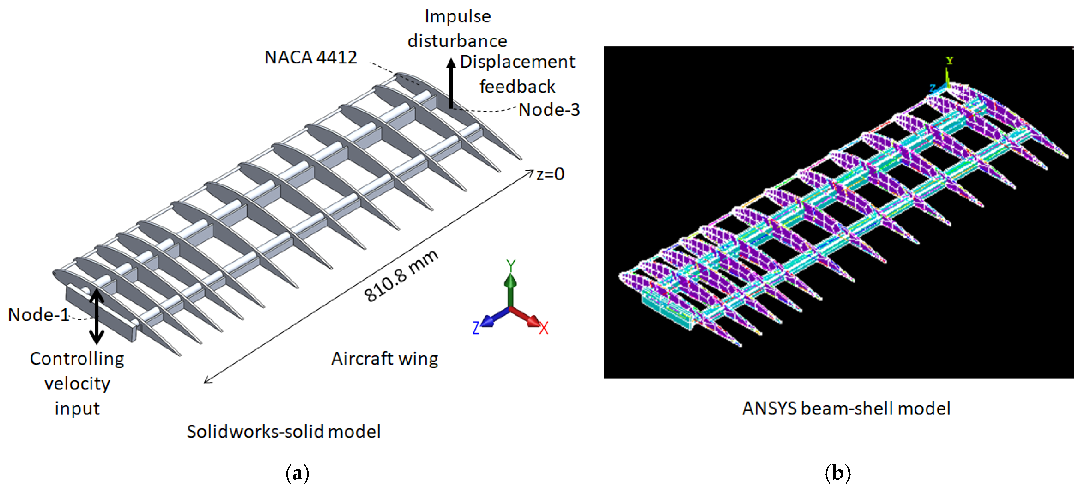
4. Simulation of Active Vibration Control of Aircraft Wing by ANSYS APDL

The simulation of the AVC of an aircraft wing by ANSYS is considered in this section. A Solidworks model of an ANSYS beam–shell model aircraft wing is shown in Figure 7, (Solidworks: 2023 Student Edition).
The geometry of NACA 4412 airfoil [26] is used to model the ribs. The length of the foil is 300 mm. The thickness of the ribs is 4.2 mm. The wing has 13 ribs. The mid-plane of Rib-1 is at z = 0. The z coordinates of the mid-axes of the 13 ribs are 0, 50.8, 130.8, 210.8, 290.8, 370.8, 450.8, 530.8, 611.4, 661.4, 711.4, 760.8, 810.8 mm, respectively. There are 5 beams along z axis. The origins of the beams located at z = 0 has the center locations (x = 5.5 mm, y = 0.6 mm), (x = 81.2 mm, y = 10.7 mm), (x = 100.6 mm, y = 6 mm), (x = 198 mm, y = 9.8 mm), (x = 211 mm, y = 5.6 mm), respectively. The beam cross-sections have shapes and dimensions as a circular pipe with D = 5 mm and tk = 0.5 mm; circular pipe with D = 16 mm and tk = 1 mm; rectangular with w = 3 mm, h = 25 mm; circular pipe with D = 14 mm and tk = 1 mm; rectangular with w = 3 mm, h = 15 mm, respectively. Here, D is the outer diameter, tk is the thickness, w is the width and h is the height. Beam-6 is used to connect the beams 2 and 4 (Beams with D = 16 mm and D = 14) with the dimensions 10 mm × 30 mm × 157.5 mm. Node-1 on Beam-6 is fixed for the Control-Off case and the controlling velocity input is applied to Node-1 for the Control-On case. The disturbance impulse is applied to Node-3 on the rib at z = 0 and the displacement feedback is gathered from the node. Node-1 and 2 are located at the centroid of the airfoil area.
In the first part of the ANSYS-APDL program, the ribs are modeled as shell FE’s (SHELL181) and the beams are modeled as beams (BEAM188) in ANSYS. The element types are defined by the et command. Material properties are defined by the mp command. Rayleigh damping coefficients are defined by the alphad and betad commands. Beam and shell sections are defined using the sectype and secdata commands. Keypoints are created using the k command at the locations of the rib foil sample coordinates and at the locations of beam centers for all the ribs. Nodes 1 and 3 are defined using the n command. Areas are created to model the ribs using the a command and the keys created. Sub-areas are used to model a rib so that the centers of the beams coincided with the corners of sub-areas. The aglue command is used to connect the sub-areas. Lines are created to model beams using l command and the keypoints created. Areas are meshed using the amesh command, and lines and beams are meshed using the lmesh command. The nummrg command is used to merge the nodes created at the same locations. The keypoints and areas created for Rib-1 at z = 0 are repeated for the subsequent 12 ribs with the same x-y coordinates and changing z coordinates, and APDL commands for this are created using VisualBASIC program (Version 6.0). The second part of the APDL program is the same as given in Section 2.4.

5. Results and Discussions

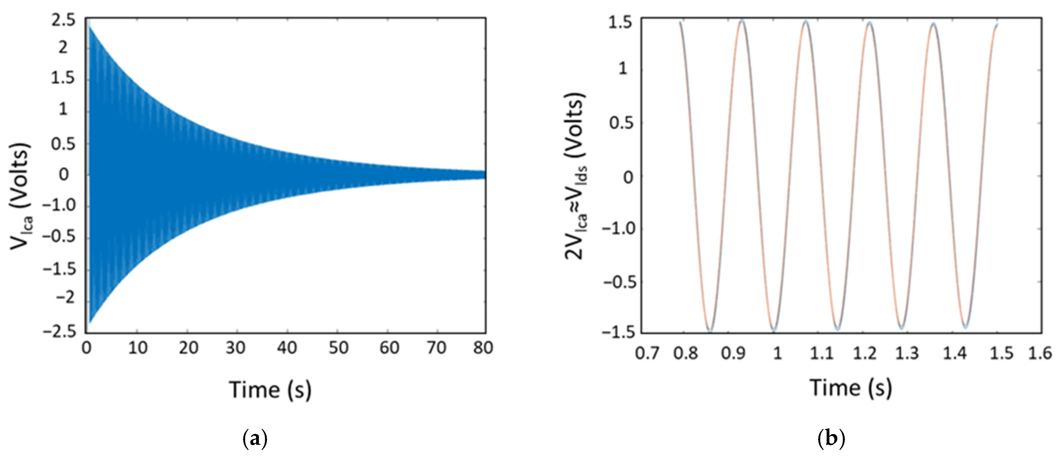
5.1. Comparison of Experimental Strain and Displacement Sensor Output Signals

The amplitude, Ad, of the impulse in the simulations is selected so that the output signal had a maximum value of 2.5 V in the solution with Laplace transform method for Control-Off case (Kp = 0). The value, 2.5 V, corresponds to 10 mm maximum mass displacement. Let the value of the maximum of the output voltage be Vp for the gain Kp for Control-On case in the solution with Laplace transform method. The impulse disturbance in the experiments are applied manually, and thus the amplitude of the impulse is unknown. It is applied in the x direction to the end mass. The maximum of the output signal is observed and the experiment is repeated if the maximum is not approximately 2.5 V. The output signal in the experiments, Vo(t), is scaled with Cp = (Vp/Vmax)Vo, where Vmax is the maximum of Vo, for comparisons. The output signals are shifted so that the time at which the first peak occurs is 0.5 s.
Let rms0 and rmsp be the rms values [24] for the output signals for Control-Off case and Control-On case for Kp. The suppression of the vibration with AVC is quantified with the relative value of rp (%) and given as rp = 100(rms0 − rmsp)/rms0.
The scaled strain output signal, Vlca, obtained from the experimental system for the free vibration of the cantilever beam after an impulse disturbance, is shown in Figure 8a. Windowed 2Vlca and Vlsd signals are shown in Figure 8b. It is observed that 2Vlca ≈ Vlds. Displacement output signals are used in the simulations because it can be implemented in analyses. ANSYS gives displacement values but, as far as the authors are aware, does not give strain values in the *do *enddo loop in the transient solutions. Strain values are obtained using etable command in the post-processing stage after the solution stage. On the other hand, displacement sensors require additional mounting for installation and are not practical in applications. Strain gauges can be easily installed and give a cost-effective solution for feedback signals. The observation in Figure 8b shows that the results obtained in simulations using the displacement feedback can be used in applications using the strain feedback.
It is noted that there is a linear relation between a single strain in the y direction at Node-4, εy, and the displacement in the x direction at Node-3, dm; and the relationship can be derived as εy = (1.5 h/L2)dm using the Bernoulli–Euler beam theory. Here, h is the thickness of the beam, and L is the distance between Node-3 and Node-4.

5.2. Determining Damping Constant Experimentally

Rayleigh damping [21] is considered in simulations. The damping matrix is defined as [C] = α[M] + β[K] where α and β are the proportional damping constants. Modal damping ratios are given as ξi = α/(2ωi) + βωi/2, where i is the i-th mode, and ωi is the i-th natural frequency. The modal damping ratio can be found using the logarithmic decrement formulation [22]. The stiffness damping only is considered in this study. The amplitude versus frequency plot obtained from the Fast Fourier Transform (FFT) [25] of the signal in Figure 8a is shown in Figure 9.
The peak values can be read on the signal in Figure 8a and it is found that the amplitude of the 3rd peak, and the amplitude of the 8th peak are 2.3209 and 2.2363, respectively. The Rayleigh stiffness damping coefficient is found as β = 5.3702 (10−5) using the logarithmic decrement formulation and it is used in simulations.

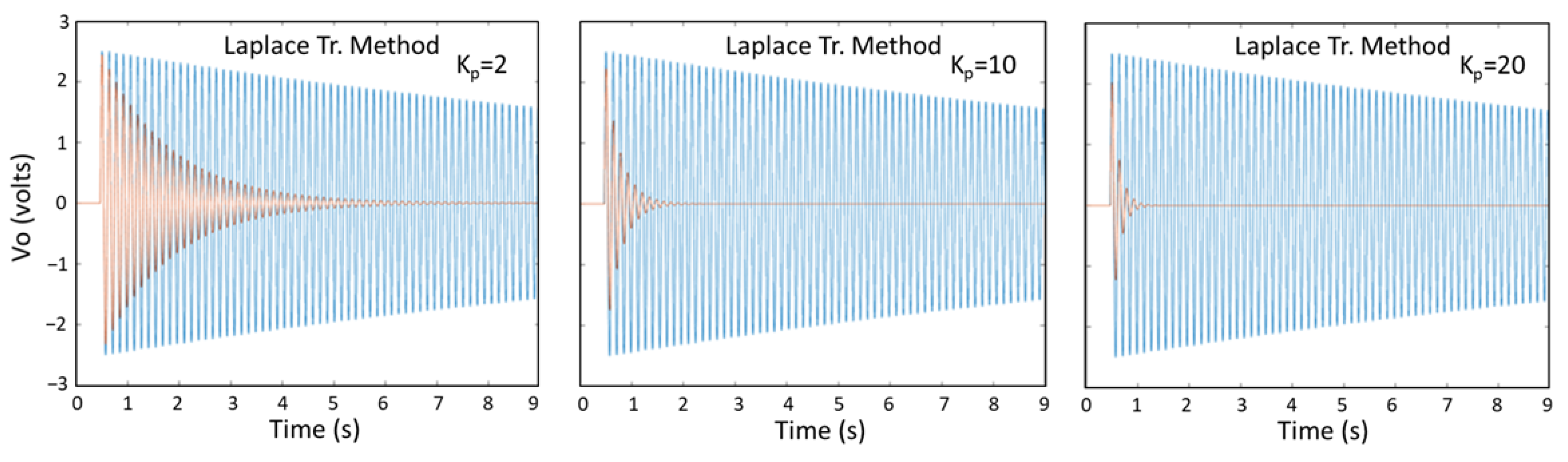
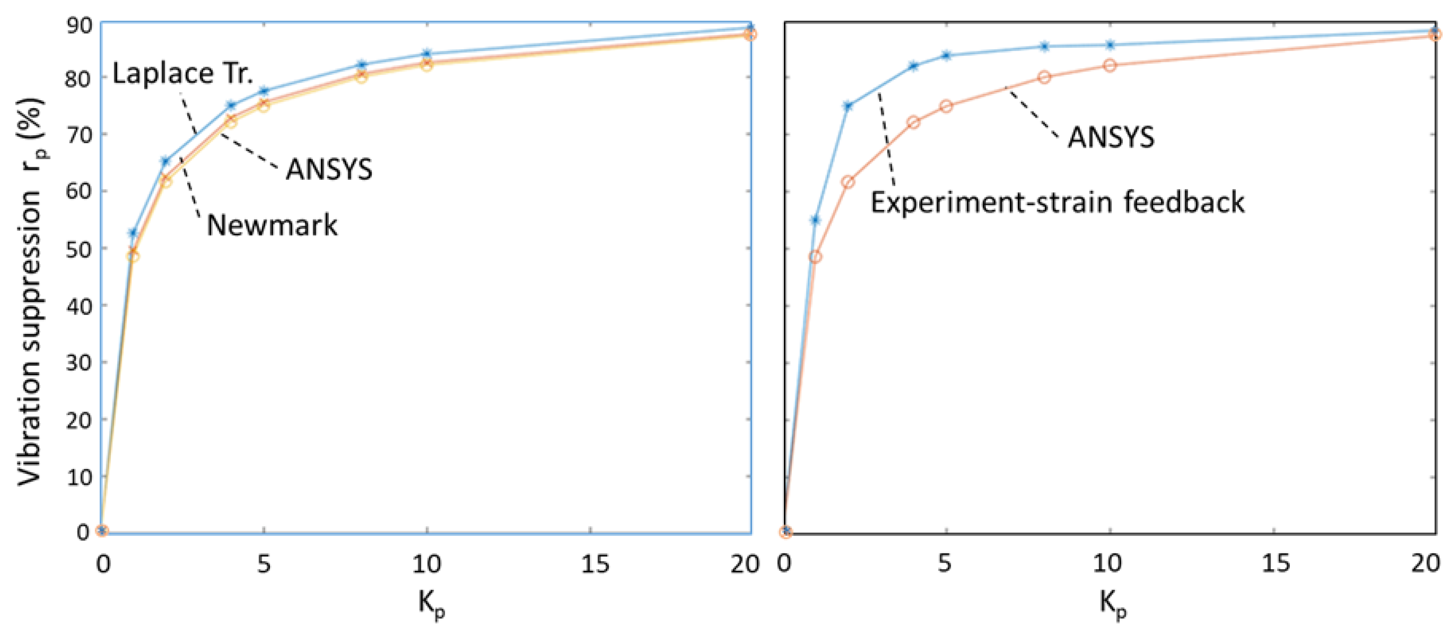
5.3. AVC of Cantilever Beam Results Obtained by the Laplace Transform Method, Newmark Method, ANSYS, and Experiments

The first and second un-damped natural frequencies obtained from the FE model given in Section 2.1 are found as f1 = 7.2222 Hz and f2 = 80.95 Hz, using the eig command in MatLAB. The computer processor and tdelay determines the sampling frequency, fs, in the experimental system. tdelay is taken as 1000 µs and fs is measured as 790.1420 Hz. The FFT gives the spectrum 0–790.1420/2 Hz and only the peak value at f = 7 Hz is observed in the spectrum as shown in Figure 9a. The corresponding spectrum obtained by the Laplace transform method is shown in Figure 9b. The second mode with f2 = 80.95 Hz is not observed in the spectra in Figure 9. This is because the impulse disturbance excites the first mode only and thus only the first mode is considered in the simulations.
The first natural frequency from the ANSYS model (Section 2.4) is found as 7.22 Hz, using modal analysis in ANSYS. It is observed that simulation and experimental results are in good agreement for the first natural frequency.
The time step, Δt, is taken as 0.005 s, which is smaller than 1/7.2222/20 = 0.0069 s, in simulations. The amplitude of the unit impulse is taken as Ad Δt in the Laplace transform method. Ad is taken as the value of the disturbance force at the time Δt and zero other time steps in the Newmark method and ANSYS. The Ad value is found as 21.989 so that the output signal had a maximum value of 2.5 V in the solution with the Laplace transform method for the Control-Off case (Kp = 0). The Vp values for scaling are found as 2.5, 2.4698, 2.4401, 2.3822, 2.3539, 2.2750, 2.2301, and 2.0237 for Kp values 0, 1, 2, 4, 5, 8, 10, and 20, respectively.
The values of K1 and K2 are taken as 0.0025 and 250; Rayleigh damping coefficients α and β values are taken as 0 and 5.3702(10−5) in simulations. The constants Cf and Ca, defined in Section 2.2, are 10224 and 128(10224), respectively, for the selected damping constants. The output signals for selected Kp values are shown in Figure 10, Figure 11, Figure 12 and Figure 13. The video for the experiments is given in the Supplementary Materials.
It is observed that the free vibrations after the impulse disturbance are suppressed with AVC (Blue lines: Control-Off, Red lines: Control-On). The rms values of the output signals are shown in Table 2.
The suppression level of vibration for different Kp values are shown in Figure 14.
It is observed that simulation results with the Laplace Transform method, Newmark method, and ANSYS are in good agreement. The experimental results are in acceptable agreement with the simulation results. The rp values approached an asymptotic value with increasing Kp. rp values are higher for experimental results than simulation results. The reason for this observation may be additional damping effects present in physical systems such as mechanical friction, looseness at connections, surface contact interactions, and internal energy losses which are not fully modeled in simulations. These effects can lead to a more rapid dissipation of vibrational energy.

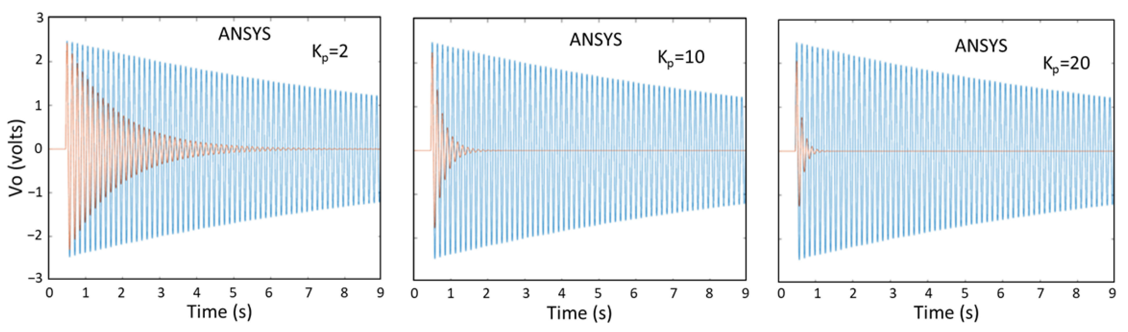
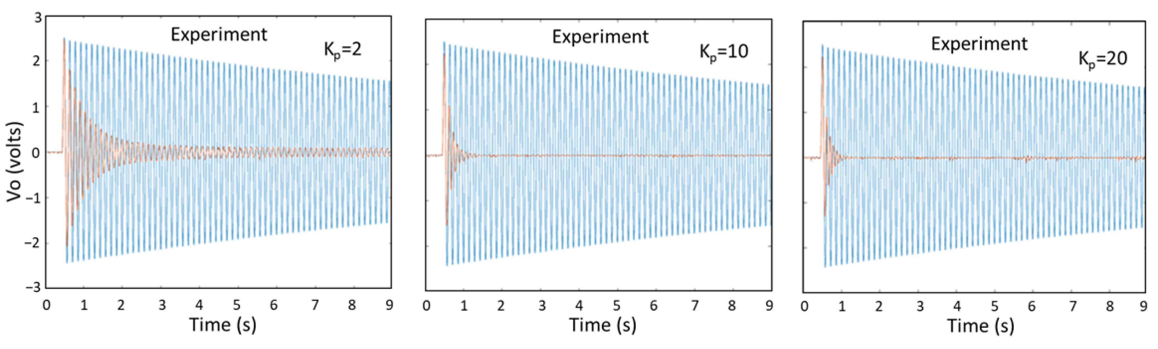
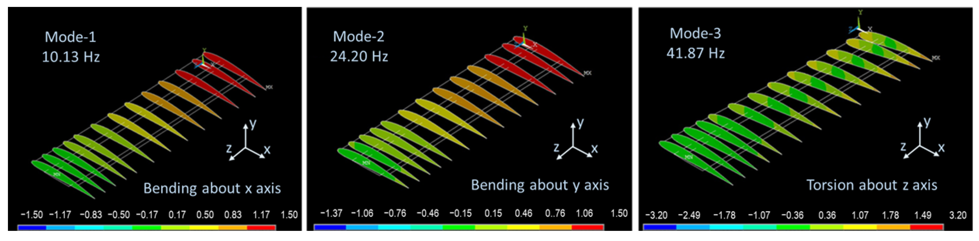
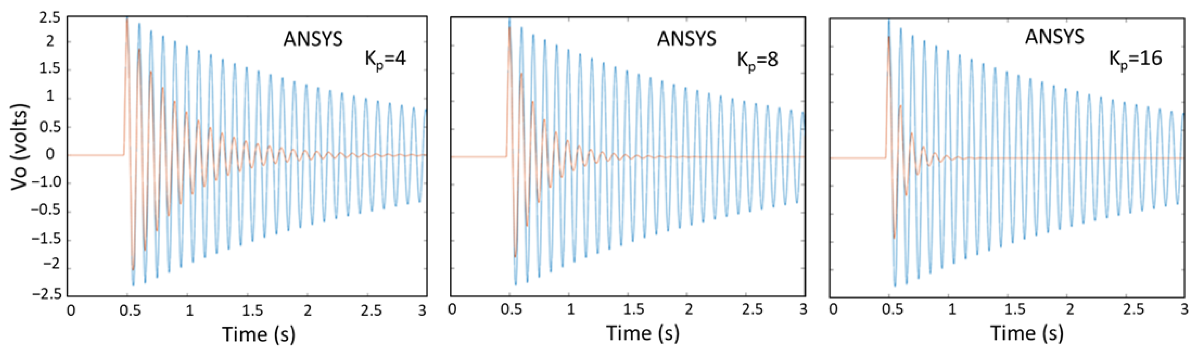
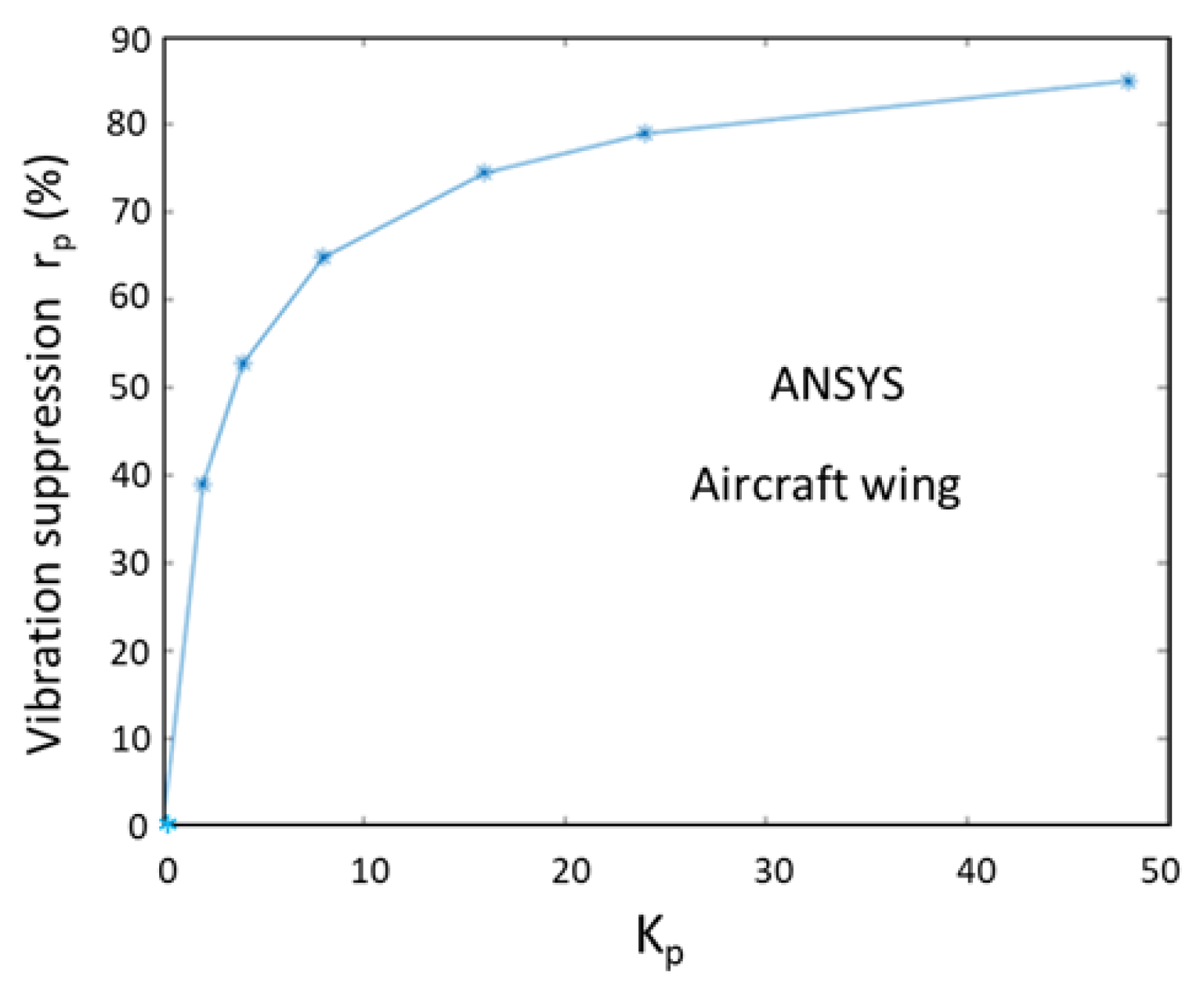
5.4. AVC of Aircraft Wing by ANSYS APDL

The APDL program developed for the AVC of the cantilever beam and verified with the results of Laplace transform and Newmark methods is extended for the aircraft wing structure given in Section 4. The smallest three natural frequencies obtained from ANSYS are f1 = 10.13, f2 = 24.20, and f3 = 41.87 Hz. Mode shapes are shown in Figure 15. Mode-1 is the bending about the x axis, Mode-2 the bending about the y axis, and Mode-3 is the torsion about the z axis.
The impulse disturbance at Node-3, shown in Figure 7, is in the y direction and excites the wing mainly as bending about x axis, and thus Mode-1 is considered for AVC.
Δt is taken as 0.004 s, which is less than 1/10.1272/20 = 0.0049 s. The experimental data for damping a wing structure is given in [27], and it is observed that the Rayleigh stiffness constant can be selected in the range of 10−4. The Rayleigh damping constants are taken as α = 0 and β = 0.0002 by inspection for the wing in this study. The amplitude, Ad, of the impulse is selected so that the output signal has a maximum value of 2.5 V. The output signals for selected Kp values are shown in Figure 16 (Blue lines: Control-Off, Red lines: Control-On).
The rms values of the output signals for the AVC of an aircraft wing are shown in Table 3 for different time steps and number of FE’s.
It is observed from Table 3 that there are small deviations with changing time step and number of finite elements. The suppression levels of vibration for the AVC of an aircraft wing for different Kp values are shown in Figure 17.
It is observed that the APDL program developed for the AVC of the cantilever beam and extended for the aircraft wing can be used successively. The rp values approach an asymptotic value with increasing Kp for the AVC of a cantilever aircraft wing as observed for the AVC of a cantilever beam with an end mass.
The aircraft wing model with multiple ribs is significantly different and more complex than the cantilever beam model. It consists of beam and shell finite elements. Its first vibration mode is a bending mode about the x axis, similar to the cantilever beam model studied. Therefore, the control approach with the developed ANSYS APDL program developed for the cantilever beam model is applicable.

6. Conclusions

In this study, we aim to study the active vibration control (AVC) of cantilever structures with ANSYS. Commercial computer-aided engineering (CAE) programs are widely used in the simulation age for analyzing real complex engineering systems. Developing mathematical models and using the Laplace transform method were the major approaches to analyzing closed loop control systems before the computer age. Graphical methods were very important, and analyses of complex real engineering systems were limited. Numerical methods like Newmark were started to be used by developing computer codes at the early age of computers. Today, commercial computer-aided engineering (CAE) programs like ANSYS enable one to model systems and define inputs only, and CAE generate the mathematical model and solve the equations for static, harmonic, and transient analyses. Developing engineering systems followed produce, test, and revise procedures before the computer age changed to simulate, revise, and produce procedures today. There is no direct modeling and solution for closed loop control systems in ANSYS. A procedure which integrates control action into the transient solution in ANSYS APDL is proposed in this study. It should be noted that one must be very careful using simulation methods because a minor mistake in the process can give erroneous results. Testing the validity of the CAE procedures by Laplace transform and numerical methods for a basic structure is important before applying it to complex structures. The Laplace transform method gives analytical solutions. The Newmark method is used for numerical solutions. The Laplace transform method and Newmark method require developing mathematical models of the system under study. The APDL method is used to obtain solutions by defining the system in the preprocessor stage. APDL develops the mathematical model of the system. The transient solution is obtained in ANSYS in the solution stage. However, the control action is integrated into the transient solution in APDL as the algorithm in the Newmark method.
In this study, a cantilever beam with an end mass is studied first. The disturbance is considered as an impulse to the end mass. The controlling action is taken as linear velocity actuation to the base, which can be generated with servo motors and servo valves. The rotational velocity actuation can be used for other applications such as robot arms. The strain signals amplified by a load-cell amplifier are considered as the feedback in the experiments. Strain feedback is cost-effective and can easily be implemented in real engineering applications. Displacement feedback is used in simulations because the displacement information can be obtained, but as far as the authors’ knowledge, the strain information cannot be obtained in the transient solution stage in ANSYS. Strain and displacement feedback signals are compared experimentally, and it is observed that there is a linear relationship between them approximately. The finite element model of a cantilever beam with end mass is developed for AVC analysis with the Laplace transform and Newmark methods. The control action is integrated to the transient solution in the Newmark method. There is no need to develop a mathematical model after defining the systems in ANSYS. The control action is integrated into the transient solution like in the Newmark method. An experimental system, which uses an Adlink-9222 PCI DAQ card and a C program is introduced. It is observed that the controlling velocity sign must be in the opposite direction of error sign.
It is concluded that the developed ANSYS procedure can be used for AVC analysis of cantilever structures. The procedure can be applied to robotic arms, flexible manipulators, antenna masts, and solar panels attached to a spacecraft. In this study, the ANSYS procedure is applied for the AVC of a cantilever aircraft wing successfully. The initial selections of sensors, actuators, and control parameters can be determined with iterations in ANSYS, and then the control parameters can be improved on produced systems using different methods such as the receptance method.
It should be noted that the disturbance signals are created manually. Also, only proportional control action is used in this study because the experimental and simulation results are satisfactory. This study can be extended for various control methods such as PI, PD, PID, or intelligent control methods. This will improve the generalizability of the results of this study. Also, the AVC of multiple input and output systems, torsional vibrations in aircraft wings, and different structures can be considered for further studies.
The novel contribution of this study is in the direct integration of closed-loop control into the transient analysis within the ANSYS APDL environment. ANSYS does not natively support control algorithms. The APDL-based control implementation developed in this study is successfully applied and cross-validated using both Laplace and Newmark methods. Also, the practical and cost-effective applicability of strain feedback using load-cell amplifiers represents an innovative contribution of this research. The results of this study can be used in various engineering applications with complex structures.

Supplementary Materials

The following supporting information can be downloaded at: https://www.mdpi.com/article/10.3390/machines13050379/s1, Video S1: Recordings of experimets for AVC of cantilever beam with end mass for different Kp values.

Author Contributions

Conceptualization, M.A. and H.K.; Methodology, M.A. and H.K.; Software, İ.B. and H.K.; Validation, İ.B. and H.K.; Formal analysis, İ.B., M.A. and H.K.; Data curation, İ.B.; Writing—original draft, İ.B. and H.K.; Writing—review & editing, İ.B. and M.A.; Supervision, M.A. All authors have read and agreed to the published version of the manuscript.

Funding

This research received no external funding.

Data Availability Statement

Data is contained within the article.

Conflicts of Interest

The authors declare no conflict of interest.

Appendix A. ANSYS APDL Code for AVC of Cantilever Beam

finish
/config,nres,10000
/clear,nostart
!----------------
b=39.3e-3
h=2e-3
mend=171e-3
Iz=b*h**3/12
ymax=h/2

Kp=10
fl='va10'
dt=0.005
tend=9
A=40
K1=0.0025
K2=250
!-----
/prep7
mp,ex,1,200e9
mp,dens,1,7900
mp,nuxy,1,0.3
alphad,0
betad,7.8e-5

et,1,beam188
keyopt,1,2,1
keyopt,1,3,3
keyopt,1,4,1
keyopt,1,6,3
keyopt,1,7,1
keyopt,1,9,1
sectype,1,beam,rect,srect1,0
secdata,h,b,2,2

et,2,mass21
r,1,mend,0,0,0,0,0

n,1,0,0
n,2,0,349/1000
n,3,0,(6+265+46)/1000
n,4,0,6/1000
n,5,0,(6+265)/1000

e,1,4
e,4,5
e,5,3
e,3,2

type,2
real,1
e,3
/eshape,1,1

d,all,uy,0
d,all,uz,0
d,all,rotx,0
d,all,roty,0
d,1,all,0

gplot
!--------------------
/solu
keyw,pr_sgui,1
/output,null

antype,trans,new
outres,all,all
kbc,0
deltim,dt

*cfopen,fl,txt
*vwrite,0,0
(E15.8,',',E15.8)

ns=tend/dt+1

*do,n,2,ns,1
 t=(n-1)*dt
 fd=0
 *if,t,eq,dt,then
  fd=As
 *endif
 f,3,fx,fd
 time,t
 solve
 *get,dm,node,3,u,x
 *get,ds,node,1,u,x
 Vo=K2*(dm-ds)
 errv=0-Vo
 vs=-K1*Kp*errv
 d,1,velx,vs
 *vwrite,t,Vo
 (E15.8,',',E15.8)
*enddo

*cfclose
finish
/post26
nsol,2,2,u,x
plvar,2

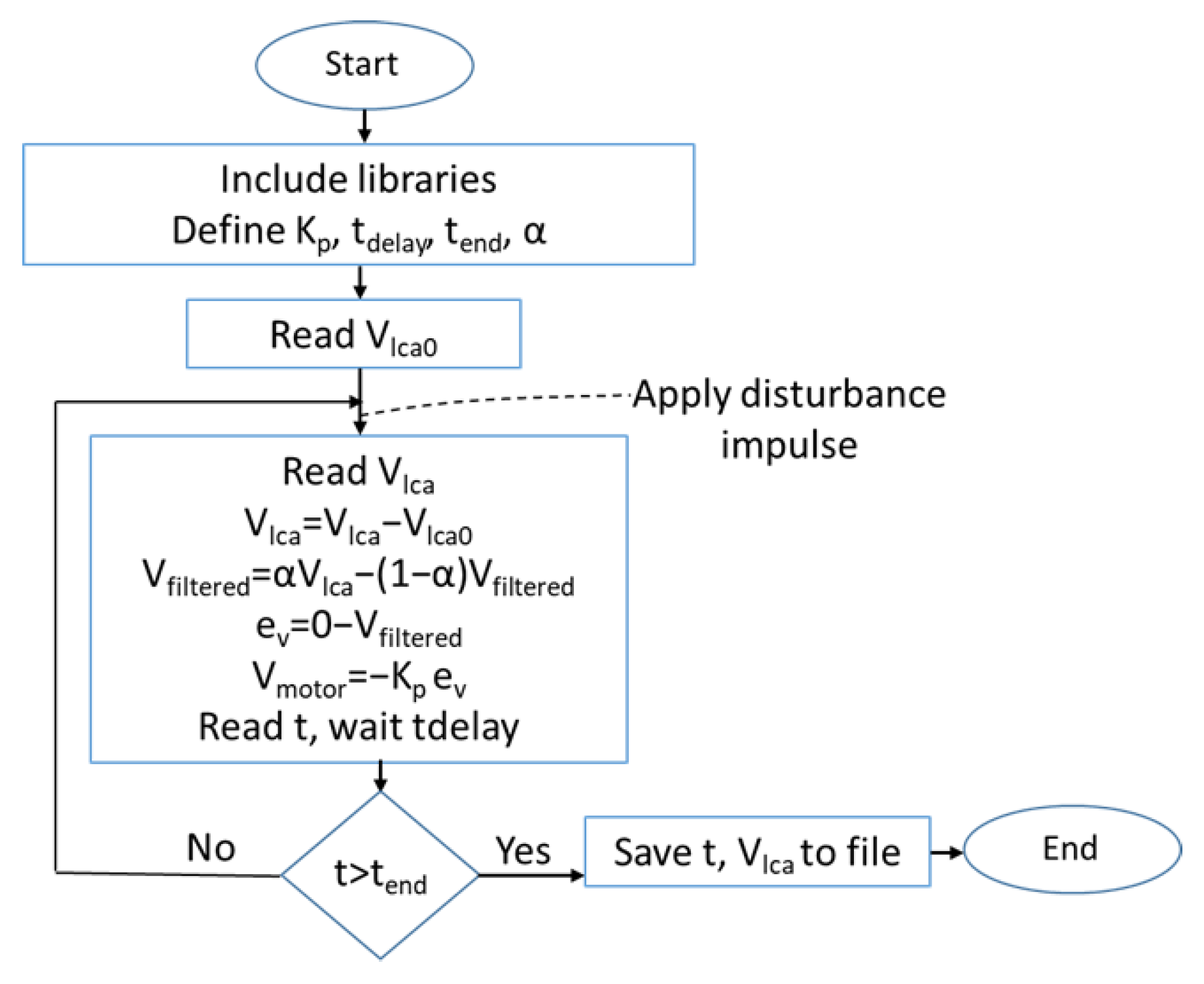
Appendix B. C Program for Experimental System

#include <stdio.h>
#include <stdlib.h>
#include <math.h>
#include <unistd.h>
#include <string.h>
#include "dask.h"
#include <time.h>
#include <conio.h>
float alpha = 0.1; // 13.9728 Hz
float Kp = 8;
int tend = 10;
float dt=1/790.1420; //dt=0.0011266
//------------------------
void pcon(float Kp, const char *flc, int tend)
{
 long tdelay = 1000, trecord = tend * 1000000, tv = 0;
 U16 card_num = 0, Chai = 1, AdRange = AD_B_10_V, Value, Chao = 1;
 float Vfiltered = 0, *Vsens = NULL, *tval = NULL;
 Vsens = (float *)calloc(1000000, sizeof(float));
 tval = (float *)calloc(1000000, sizeof(float));
 FILE *fl;
 struct timespec t0, t;
 int n, ns = 0;
 I16 card, err;
 F64 Vsensor, Vsensor0, Vmotor;
//---
 card = Register_Card(PCI_9222, card_num);
 err = AO_VWriteChannel(card, Chao, 0);
 err = AI_ReadChannel(card, Chai, AdRange, &Value);
 AI_VoltScale(card, AdRange, Value, &Vsensor0);
 clock_gettime(CLOCK_MONOTONIC_RAW, &t0);
 printf("%f %f %s \n", Kp, alpha, flc);

 do
 {
  ns = ns + 1;
  err = AI_ReadChannel(card, Chai, AdRange, &Value);
  AI_VoltScale(card, AdRange, Value, &Vsensor);
  Vsensor = Vsensor - Vsensor0;
  if (ns == 0) Vfiltered = Vsensor;
  if (ns > 1) Vfiltered = alpha * Vsensor + (1 - alpha) * Vfiltered;
  Vsensor = Vfiltered;
  Vsens[ns] = Vsensor;

  float errv = 0-Vsensor;
  Vmotor = -Kp * errv;
  if (Vmotor > 10.0) Vmotor = 10.0;
  if (Vmotor < -10.0) Vmotor = -10.0;
  err = AO_VWriteChannel(card, Chao, Vmotor);
  clock_gettime(CLOCK_MONOTONIC_RAW, &t);
  tv = (t.tv_sec - t0.tv_sec) * 1000000L + (t.tv_nsec - t0.tv_nsec) / 1000;
  tval[ns] = tv / 1000000.0;
  usleep(tdelay);
  if (tv > trecord) break;
 } while (!kbhit());

 err = AO_VWriteChannel(card, Chao, 0);
 Release_Card(card);
 fl = fopen(flc, "w");
 for (n = 1; n < ns; n = n + 1)
 {
  fprintf(fl, "%f %f \n", tval[n], Vsens[n]);
 }
  fclose(fl);
  free(Vsens);
  free(tval);
}
//---------------------
void countdown(const char *message, int seconds)
{
 for (int i = seconds; i > 0; i--)
 {
  printf("%s in %d seconds…\r", message, i);
  fflush(stdout);
  sleep(1);
 }
 printf("%s now starting…\n", message);
}

//---------------------------------------------------------
int main(int argc, char **argv)
{
 countdown("Starting Control ON", 3);
 pcon(Kp, "vcon.txt",tend);
  FILE *gp = popen("gnuplot -persist", "w");
 fprintf(gp,"plot '%s' with lines \n", "vcon.txt");
 return 0;
}

References

  1. Wang, Y.; Wu, W.; Lou, X.; Görges, D. Adaptive vibration control for stabilisation of the Euler–Bernoulli beam with an unknown payload. Int. J. Control 2024, 1–12. [Google Scholar] [CrossRef]
  2. Lyu, Z.; Li, C.; Jia, T. Combined vibration control of flexible cantilever beam driven by MFC actuators and rotary motor. Acta Mech. 2024, 236, 305–320. [Google Scholar] [CrossRef]
  3. Li, W.; Yang, Z.; Li, K.; Wang, W. Hybrid feedback PID-FxLMS algorithm for active vibration control of cantilever beam with piezoelectric stack actuator. J. Sound Vib. 2021, 509, 116243. [Google Scholar] [CrossRef]
  4. Amer, Y.A.; EL-Sayed, A.T.; Abd EL-Salam, M.N. A suitable active control for suppression the vibrations of a cantilever beam. Sound Vib. 2022, 56, 89–104. [Google Scholar] [CrossRef]
  5. Saif, A.W.A.; Mohammed, A.A.; AlSunni, F.; El Ferik, S. Active Vibration Control of a Cantilever Beam Structure Using Pure Deep Learning and PID with Deep Learning-Based Tuning. Appl. Sci. 2024, 14, 11520. [Google Scholar] [CrossRef]
  6. Huang, Z.; Huang, F.; Wang, X.; Chu, F. Active vibration control of composite cantilever beams. Materials 2022, 16, 95. [Google Scholar] [CrossRef]
  7. Djokoto, S.S.; Dragašius, E.; Jūrėnas, V.; Agelin-Chaab, M. Controlling of vibrations in micro-cantilever beam using a layer of active electrorheological fluid support. IEEE Sens. J. 2019, 20, 4072–4079. [Google Scholar] [CrossRef]
  8. Cui, M.; Liu, H.; Jiang, H.; Zheng, Y.; Wang, X.; Liu, W. Active vibration optimal control of piezoelectric cantilever beam with uncertainties. Meas. Control 2022, 55, 359–369. [Google Scholar] [CrossRef]
  9. Umar, H.M.; Zhang, L.; Yu, R.; Gao, Z. Improved active vibration control of a cantilever beam using MFC actuators with Hammerstein model-based hysteresis modeling and VSS-FxLMS control algorithm. J. Low Freq. Noise Vib. Act. Control. 2024, 21, 14613484241295460. [Google Scholar] [CrossRef]
  10. Teoh, J.Q.; Tehrani, M.G.; Ferguson, N.S.; Elliott, S.J. Eigenvalue sensitivity minimisation for robust pole placement by the receptance method. Mech. Syst. Signal Process. 2022, 173, 108974. [Google Scholar] [CrossRef]
  11. Karagülle, H.; Malgaca, L.; Öktem, H.F. Analysis of active vibration control in smart structures by ANSYS. Smart Mater. Struct. 2004, 13, 661. [Google Scholar] [CrossRef]
  12. Ito, T.; Tagami, M.; Tagawa, Y. Active vibration control for high-rise buildings using displacement measurements by image processing. Struct. Control Health Monit. 2022, 29, e3136. [Google Scholar] [CrossRef]
  13. Ramírez-Neria, M.; Morales-Valdez, J.; Yu, W. Active vibration control of building structure using active disturbance rejection control. J. Vib. Control 2022, 28, 2171–2186. [Google Scholar] [CrossRef]
  14. Gheni, E.Z.; Al-Khafaji, H.M.; Alwan, H.M. A deep reinforcement learning framework to modify LQR for an active vibration control applied to 2D building models. Open Eng. 2024, 14, 20220496. [Google Scholar] [CrossRef]
  15. Zhang, Q.; Han, S.; El-Meligy, M.A.; Tlija, M. Active control vibrations of aircraft wings under dynamic loading: Introducing PSO-GWO algorithm to predict dynamical information. Aerosp. Sci. Technol. 2024, 153, 109430. [Google Scholar] [CrossRef]
  16. He, T.; Zhu, G.G.; Swei, S.S.M.; Su, W. Smooth-switching LPV control for vibration suppression of a flexible airplane wing. Aerosp. Sci. Technol. 2019, 84, 895–903. [Google Scholar] [CrossRef]
  17. Li, W.; Yang, Z.; Liu, K.; Wang, W. MIMO multi-frequency active vibration control for aircraft panel structure using piezoelectric actuators. Int. J. Struct. Stab. Dyn. 2023, 23, 2350157. [Google Scholar] [CrossRef]
  18. Dong, L.; Chen, Z.; Sun, M.; Sun, Q. Phase compensation active disturbance rejection control for shimmy vibration with magnetorheological damper of aircraft. Expert Syst. Appl. 2023, 213, 119126. [Google Scholar] [CrossRef]
  19. Sahin, M.; Karadal, F.M.; Yaman, Y.; Kircali, O.F.; Nalbantoglu, V.; Ulker, F.D.; Caliskan, T. Smart structures and their applications on active vibration control: Studies in the Department of Aerospace Engineering, METU. J. Electroceramics 2008, 20, 167–174. [Google Scholar] [CrossRef]
  20. Prakash, S.; Kumar, T.R.; Raja, S.; Dwarakanathan, D.; Subramani, H.; Karthikeyan, C. Active vibration control of a full scale aircraft wing using a reconfigurable controller. J. Sound Vib. 2016, 361, 32–49. [Google Scholar] [CrossRef]
  21. Bathe, K.J. Finite Element Procedures, 2nd ed.; Prentice-Hall: Hoboken, NJ, USA, 2014. [Google Scholar]
  22. Rao, S.S. Mechanical Vibrations in SI Units, 6th ed.; Pearson Education Limited: Chennai, India, 2018; 1147p. [Google Scholar]
  23. Yavuz, Ş.; Akdağ, M.; Karagülle, H. A fast processing method to perform transient analysis for vibration control. Simul. Model. Pract. Theory 2020, 104, 102152. [Google Scholar] [CrossRef]
  24. Figliola, R.S.; Beasley, D.E. Theory and Design for Mechanical Measurements, 15th ed.; John Wiley & Sons: Hoboken, NJ, USA, 2011. [Google Scholar]
  25. Tan, L. Digital Signal Processing; Elsevier: Amsterdam, The Netherlands, 2008. [Google Scholar]
  26. Available online: http://airfoiltools.com/airfoil/details?airfoil=naca4412-il (accessed on 3 January 2025).
  27. Brown, J.D.; Mustafa, M.; Moore, K.J. Vibration mitigation of a model aircraft with high-aspect-ratio wings using two-dimensional nonlinear vibration absorbers. Int. J. Non-Linear Mech. 2024, 167, 104878. [Google Scholar] [CrossRef]
Figure 1. Cantilever beam structure.
Machines 13 00379 g001
Figure 2. Open loop block diagram.
Machines 13 00379 g002
Figure 3. Closed loop block diagram.
Machines 13 00379 g003
Figure 4. Flow chart for AVC of cantilever beam with the Newmark method.
Machines 13 00379 g004
Figure 5. Experimental system.
Machines 13 00379 g005
Figure 6. Flow chart of experimental AVC with Adlink-9222.
Machines 13 00379 g006
Figure 7. (a) SolidWorks model and (b) ANSYS beam–shell model of the aircraft wing.
Machines 13 00379 g007
Figure 8. (a) Scaled strain output signal (Vlca) and (b) windowed 2 × strain output signal (2 × Vlca) and laser displacement sensor output signal (Vlds) for the experimental Control-Off case.
Machines 13 00379 g008
Figure 9. Amplitude versus frequency plots of FFT of (a) the experimental signal in Figure 8a and (b) the corresponding simulation signal obtained by the Laplace Transform method.
Machines 13 00379 g009
Figure 10. Plots of AVC of cantilever beam with simulations by the Laplace Transform Method.
Machines 13 00379 g010
Figure 11. Plots of AVC of cantilever beam with simulations by the Newmark Method.
Machines 13 00379 g011
Figure 12. Plots of AVC of cantilever beam with simulations by ANSYS.
Machines 13 00379 g012
Figure 13. Plots of experimental AVC of cantilever beam.
Machines 13 00379 g013
Figure 14. Suppression level of vibration for different Kp values.
Machines 13 00379 g014
Figure 15. Mode shapes of aircraft wing.
Machines 13 00379 g015
Figure 16. Plots of AVC of aircraft wing with simulations by ANSYS.
Machines 13 00379 g016
Figure 17. Suppression level of vibration for AVC of aircraft wing for different Kp values.
Machines 13 00379 g017
Table 1. FE Assembly table.
FENodesH (mm) φ (deg)Assembly
1(1)–(4)690*13, *14, *15, 7, 8, 9
2(4)–(5)265907, 8, 9, 10, 11, 12
3(5)–(3)469010, 11, 12, 4, 5, 6
4(3)–(2)32904, 5, 6, 1, 2, 3
Table 2. rms values of output signals.
Kp = 0Kp = 1Kp = 2Kp = 4Kp = 5Kp = 8Kp = 10Kp = 20
Experiment1.31900.59300.33070.23800.21460.19340.19000.1565
Laplace Tr.1.39690.66270.48590.35010.31430.24990.22400.1590
Newmark1.26670.63850.47460.34470.31010.24720.22170.1577
ANSYS1.24840.64170.47870.34840.31250.25010.22440.1597
Table 3. The rms values of output signals for AVC of an aircraft wing for different time steps and number of FE’s.
Kp = 0Kp = 2Kp = 4Kp = 8Kp = 16Kp = 24Kp = 48
ANSYS 11.00470.61270.47470.35380.25750.21240.1520
ANSYS 21.03720.62100.47900.35600.25880.21350.1533
ANSYS 31.00510.61280.47470.35380.25750.21240.1520
1 428 finite elements (element size = 0.1), Δt = 0.004 s, simulation time = 40.2 s. 2 428 finite elements (element size = 0.1), Δt = 0.002 s, simulation time = 87.1 s. 3 2096 finite elements (element size = 0.01), Δt = 0.004 s, simulation time = 129.2 s.
Disclaimer/Publisher’s Note: The statements, opinions and data contained in all publications are solely those of the individual author(s) and contributor(s) and not of MDPI and/or the editor(s). MDPI and/or the editor(s) disclaim responsibility for any injury to people or property resulting from any ideas, methods, instructions or products referred to in the content.

