Abstract
As electric vehicles (EVs) are growing, the fault diagnosis in their drive motor becomes more important to have optimal performance and safety. Traditional fault detection methods suffer mainly from high false positive and false negative rates, computational complexity, and lack of transparency in decision-making methods. In addition, existing models are also heavy and inefficient. A lightweight framework for fault diagnosis in EV drive motors is presented with the aid of Recursive Feature Elimination with Cross-Validation (RFE-CV), parameter optimization, and in-depth preprocessing. We further optimize the models and their combination to a hybrid Soft Voting Classifier. These techniques were applied to a dataset of 40,040 data entries that had been simulated by a Variable Frequency Drive (VFD) model. We evaluated eight machine learning models, and our proposed Soft Voting Classifier has the highest test accuracy of 94.52% and a Kappa score of 0.9210 on diagnostic performance. Also, the model has minimal memory usage and low inference latency. In addition, Local Interpretable Model-Agnostic Explanations (LIME) were used to improve transparency and gain an understanding of decisions made through the Soft Voting Classifier. Also, the framework was validated by an additional real-world dataset, thereby further confirming its robustness and consistency in performance for different conditions, which indicates the generalizability of the framework in real-world applications. RFE-CV is found to be very effective in feature selection and helps to construct a lightweight and cost-effective ensemble voting model for enhancing fault diagnosis for EV Drive Motors, overcoming its unsatisfactory transparency, accuracy, and computational efficiency. Finally, it contributes to the development of safer and more reliable EV systems through the development of models supervised on fewer features to give the computing time that is a little lighter without compromising its diagnostic performance.
1. Introduction
The global electric vehicle (EV) market is currently experiencing a major transformation because analysts forecast substantial sales growth during the upcoming years. The analysis from Rho Motion indicates that EV sales will grow by 17–18% to exceed 20 million units during 2025 [1,2,3]. The EV market’s expansion mainly stems from the predicted EV unit numbers of 12.9 million in China, 3.5 million in Europe, and 2.1 million in North America. When EV adoption continues its quick momentum, it becomes clear that sustainable transportation is becoming essential since late detection of motor system faults might trigger life-threatening incidents [4]. Short circuits alongside demagnetization-related electrical problems lead to unexpected loss of control, which threatens both the driver’s safety and traffic users [5]. The predictions from analysts indicate electric vehicles will capture between 25% of global vehicle sales by 2025 because of their role in clean energy adoption [6].
The fast-paced EV sector introduces complex obstacles for maintaining dependable performance and safety standards of these vehicles. The correct functioning of electric vehicle motor drives stands as a crucial area for diagnosis since they play a key role in delivering vehicle performance. These systems, composed of battery management and motor drive components, become complicated and difficult to handle during fault events. Vehicle performance becomes degraded while accident risk increases and operational lifespan decreases due to common faults such as phase-to-phase faults, overvoltage, overload, and undervoltage conditions. The accurate functioning of fault detection systems is essential to preserve EV safety together with the performance and longevity of their operational lifespan.
Current fault diagnosis systems operate with multiple severe constraints in their approach. Conventional systems suffer from errors during decision-making along with slow runtimes while revealing minimal clarity about their decision-making methods [7]. These diagnostic methods remain inadequate for field implementation because fast and light solutions with high efficiency represent today’s deployment requirements. The existing fault diagnosis methods demonstrate prohibitive shortcomings that necessitate creating an innovative method to improve EV system reliability in an expanding and complex landscape.
The presented research develops a modern, lightweight framework that diagnoses faults within EV motor drives. The framework strengthens data quality through advanced preprocessing procedures, which allow the fault detection operation to function with accuracy. The study adopts Recursive Feature Elimination with Cross-Validation (RFE-CV) to select features, and this approach simultaneously improves model performance and lowers computational requirements. The deployment of the Soft Voting Classifier as part of the hybrid ensemble learning approach allows both better diagnostic precision and reduced operational expenses in model operation. The framework includes the Local Interpretable Model-Agnostic Explanations (LIME) functionality for model decision-process transparency enhancement.
Although this study is not meant for real-time deployment, its lightweight and fast training methods provide its qualities for the real application in the fast-growing EV industry. The contributions of this research are towards the advancement of EV fault diagnosis with a scalable, reliable, and efficient system for fault detection that is accurate while computationally efficient. Below, the contribution of this research is provided:
- Data preprocessing was carried out in-depth to intensify the quality of data and increase the accuracy of fault detection.
- Recursive Feature Elimination (RFE-CV) with Cross-Validation is used to select the best features. This keeps the model efficient and lightweight.
- The framework improves motor fault detection by finding the best configuration from different sets of hyperparameters.
- The use of regularization parameters mitigates overfitting, and leakage of the data is handled in order to enable the model to be robust and reliable in the real-world use case.
- A Soft Voting approach is used to extend diagnostic accuracy at a reduced computational cost as a hybrid ensemble classifier.
- The framework is then extended to incorporate LIME to further improve transparency and understanding of the model decision-making process.
- A lightweight, reliable, and efficient detection framework to detect EV motor faults and for use in the large developing market of electric vehicles is finally proposed.
- A practical framework for real-world data, further validated through real-world datasets, too.
In summary, this paper presents a comprehensive and innovative approach to EV motor fault diagnosis, emphasizing the importance of model efficiency, accuracy, and transparency for real-world applications in the expanding electric vehicle market.
2. Related Works
Studies regarding fault diagnosis of EV motors and other motor types are reviewed in this section. Mechanisms like machine learning, deep learning, and hybrid methods are studied in the different methods that are used to detect motor faults. Moreover, the limitations of these studies, including such validations, overfitting, and generalizability, are presented in the review to provide insights into the state of the art of motor fault diagnosis research.
Studies on fault classification in electric vehicle drive motors are presented by Thirunavukkarasu et al. with a remarkable accuracy of 94.1% in the case of the CatBoost model [8]. Results from the research highlight the importance of developing reliable and safe electric drive fault diagnosis to improve reliability and safety. Yet, there are some limitations of this study, such as a lack of external validation, no systematic outlier removal, and unresolved data imbalance issues. Furthermore, the lack of XAI techniques does not make the prediction of the model interpretable, which is a prerequisite for practical applications in real world environments.
Faiz Ahmad et al. provide a review of AI approaches to motor fault detection and state CNN-LSTM has 97% accuracy [9]. In addition, the study is lacking in key validation methods, such as cross-validation, hyperparameter tuning, and overfitting checks, resulting in questionable results. Preprocessing, real-world applicability, and deployment challenges are all not discussed by them. Furthermore, the paper is further weakened through the missing figures and missing, fragmented explanations. Results are of little practical value because they were not validated, and there was no methodological rigor.
In their paper, Mahbub Ul Islam Khan et al. provide a wide analysis of fault detection and classification in electric vehicles (EVs) by using machine learning (ML) methods [10]. It, therefore, deals with double-line and three-line faults associated with the critical association between a three-phase inverter and a brushless DC motor. Malachi was developed with different ML classifiers, including Decision Tree, Logistic Regression, and Voting Classifier, and their accuracy and reliability were tested and measured to be very high. The models for fault types discussed in the study do have limitations, such as their lack of applicability to other fault types and the necessity for further real-world data matching to validate the models.
Prediction of induction motor faults using machine learning techniques is presented by Abdulkareem et al. to fill the vacuum between normal time spent in predictive maintenance [11]. To analyze the dataset of healthy and faulty conditions of induction motors, the research employs various machine learning algorithms, including Random Forest, Artificial Neural Networks, k-Nearest Neighbors, and Decision Trees. The Random Forest model achieved the highest accuracy of 91%, and the ANN and k-NN models had the highest accuracy of 90%. The study, however, is restricted by examined fault conditions that may limit the generalizability of the findings.
In Muhammad Samiullah et al.’s study, machine learning is used to predict preventative maintenance in induction motors, and the authors state that the Decision Tree produced the highest accuracy (92%) for detecting faults [12]. Nevertheless, the paper just gives this binary classification and does not provide insight into the entire spectrum of motor fault types. Despite the good behavior for the selected faults by the study, fault coverage does not extend beyond the selected faults, which makes the general workability of the model questionable. Incorporating additional fault types and making the model more flexible will help boost its investigation in the real world.
In the work of Debshree Bhattacharya et al., a fault detection approach is proposed based on a two-layer machine learning [13]. LGBM achieves 100% accuracy, but they are not cross-validated, explainable AI, and not regularized, causing worries of overfitting. The study is limited to simulated data for which generalizability is limited and is not fully explored for the effect of feature selection on model performance. These limitations have to be addressed, and has to be a test in the real world.
Under electric vehicle induction motor fault detection, Raziq Yaqub et al. consider engine sound and vibration data [14]. With artificial intelligence, specifically the Random Forest classifier, they reach 92% accuracy and 86–91% precision related to faults in different sizes. A notable limitation, however, is that the study is limited to the application of this idea to problems involving binary classification only and does not allow for simultaneous treatment of multiple fault types. Its applicability to more complex, real-world scenarios where simultaneous multiple faults occur limits the robustness of the system in case of diverse conditions.
In the work of Min Chan et al., the authors present a highly accurate fault diagnosis system for induction motors with 100% accuracy for SVM and CNN models [15]. The problem is that given the perfect performance, it is natural to worry about potential overfitting, as the models may be too much in tune with the training dataset, not generalizing well. Real-world testing is essential to validate the findings, as they have to take into account the complexities with variables in operation that are different from the controlled setup used during the study. This validation would make these models more applicable in industrial settings.
The work of Aniqua et al. employs XAI techniques of LIME and SHAP to further improve the interpretability and accuracy of the model when diagnosing machine faults using audio sensor data [16]. Twenty-nine features extracted from audio recordings of industrial fans were used by the authors, where a number of machine learning classifiers, such as logistic regression, XGBoost, SVM, Gaussian Naive Bayes, and Random Forest, were employed to classify the faults in the system. Using XAI as a feature, their proposed method improved the diagnostic accuracies: 80.28 for Logistic Regression with XAI and 79.57 without XAI. Nevertheless, the study’s dataset could not be diverse enough; there are issues regarding the real-time application, and audio data can be interfered with by noise. In addition, PCA suffers from limitations of linearity; hence, in cases of datasets with nonlinear relations, we may lose critical information.
The InceptionV3 with an SE attention mechanism by Lifu et al. results in a 100% detection rate; however, such an approach suffers from an overfitting problem and yields a long training time, which makes the model lengthy. Furthermore, the model is a “black box” in nature, which reduces interpretability, possibly hindering the actual use case [17]. A study is presented that utilizes 369 thermal images of an industrial motor with 11 fault types after CLAHE preprocessing. It is recognized in the study that practical limitations such as resolution constraints are associated with high-resolution images while improving accuracy.
Now, the Table 1 summarizes the limitations of previous studies along with the data types used in the dataset.

Table 1.
Summary of studies on fault detection in electric motors.
3. Methodology
This section describes a systematic approach to motor fault classification with a focus on important techniques such as Explanatory Data Analysis, Data Preprocessing, and Feature Selection. Furthermore, electric vehicle motor fault diagnosis is integrated with advanced machine learning models and explainable AI (XAI) to further improve the accuracy and reliability of the diagnosis. This helps with effective and trustworthy fault detection.
3.1. Data Collection
This simulated dataset for experiment 1 used in this study was collected from GitHub [18]. It is generated using a Variable Frequency Drive (VFD) model simulated in MATLAB Simulink. In total, the dataset had 40,040 entries and a total of nine features, as well as a target column. One of the ten columns was an object, and nine others were numerical. The target column has a total of six classes. Also, the framework was further validated on another similar dataset used in experiment 2 to see whether the framework is effective for an empirical dataset or not [19]. This dataset has a total of nine classes. Section 4.2 presents the results based on this dataset.
Table 2 shows the description of the features, while Table 3 lists the faults and their counts for each fault for the MATLAB dataset.
Table 2.
Feature description.
Table 3.
Fault descriptions and their counts.
3.2. Explanatory Data Analysis
This section presents EDA (Exploratory Data Analysis) [20]. It helps us to understand the dataset’s structure, distribution, and relationships between variables. It also helps us understand the data, ensuring quality and integrity. Both are key for building accurate, reliable predictive models.
3.2.1. Descriptive Statistics
In Table 4, it is found that the ‘Ia (Amp)’ and ‘Torque (N-m)’ features show the widest ranges. Also, ‘Torque’ includes both negative and positive values. There are also variations in features such as ‘Vab (V)’ and ‘Speed (rad/s)’.
Table 4.
Summary statistics: min, max, range, and average values for each feature.
3.2.2. Distribution Characteristics
The skewness and kurtosis [21] values for each characteristic are presented in Table 5. Skewness measures the asymmetry of a distribution. For instance, features like Tn and k are right-skewed. Kurtosis specifies the tails of a distribution. High kurtosis values, such as Torque and Ia, suggest a heavy-tailed distribution.
Table 5.
Skewness and Kurtosis values for each feature.
3.2.3. Histographic Representation
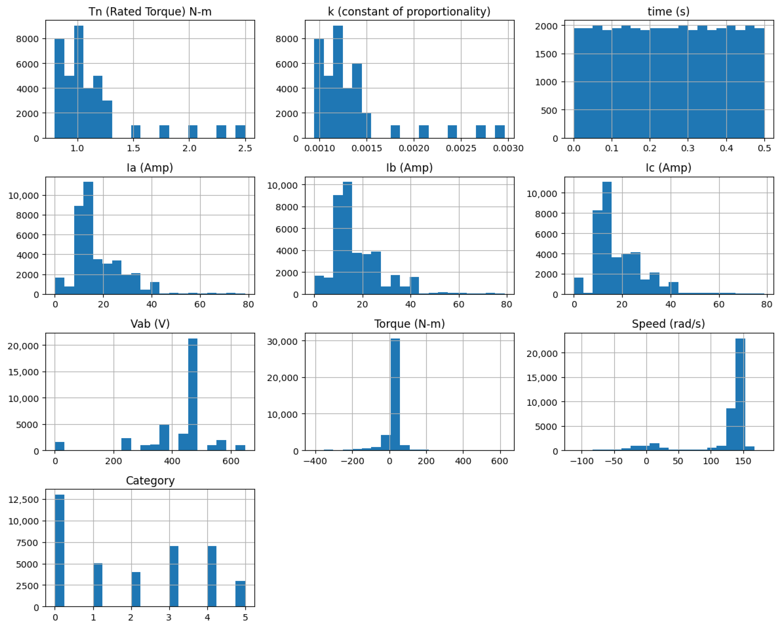
Figure 1 displays histograms for all features and reveals fluctuations in the rated torque (Tn), phase currents (Ia, Ib, Ic), voltage (Vab), torque (T), and speed (n). The histograms show how these parameters change during the process. Time shows a consistent pattern, while other parameters vary. This pattern shows a strong relationship between these key metrics in the system.

Figure 1.
Histogram of the data distribution.
3.2.4. Outlier Detection
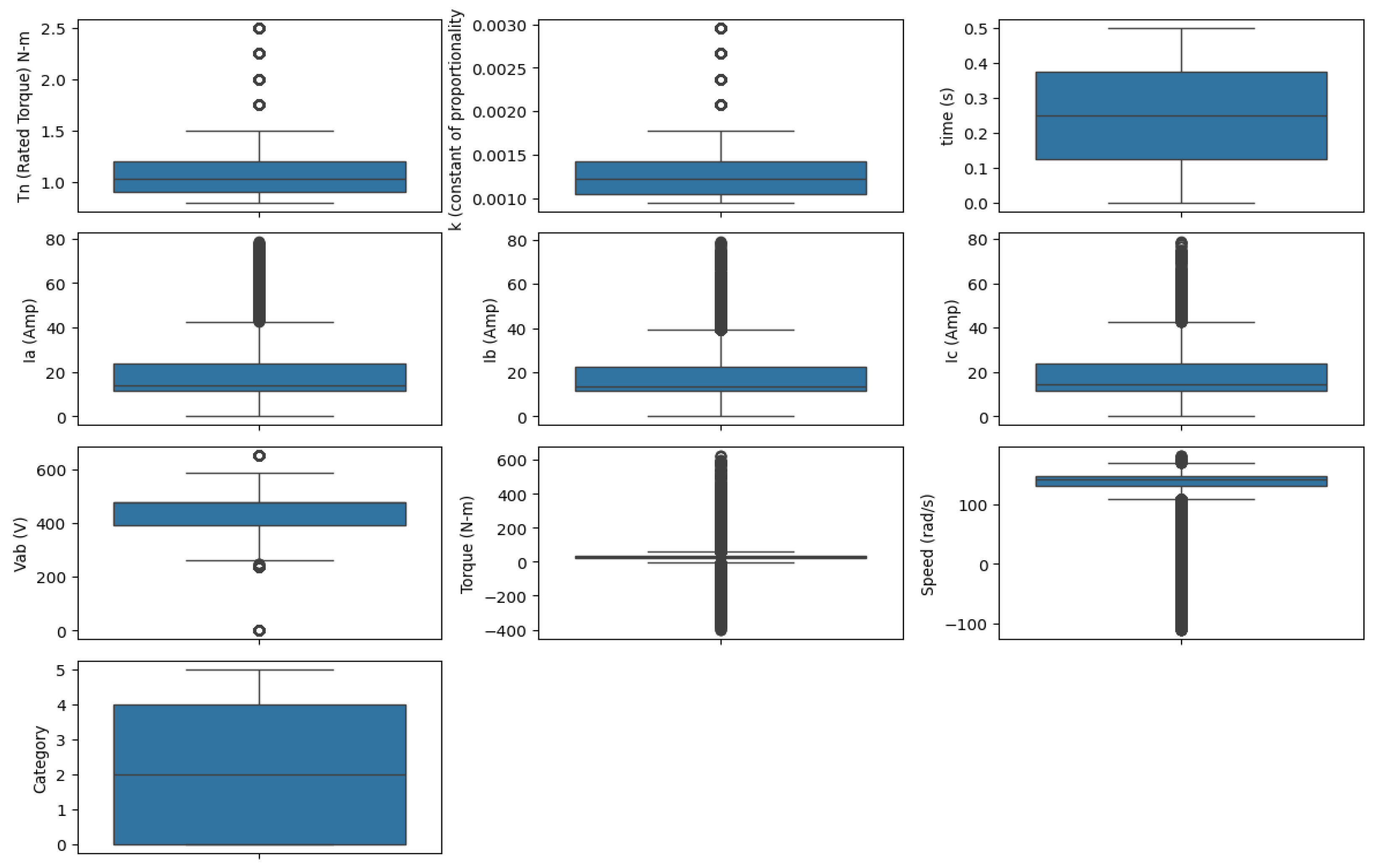
Figure 2 displays the distribution of the features. It includes central tendency, variability, and outliers. It highlights that all features, except time (s), have outliers. Time remains constant and has no outliers. The whiskers and IQRs for torque, current, voltage, and speed show significant variation. This indicates more dynamic fluctuations in the data.

Figure 2.
Box plot of all features.
3.2.5. Correlation Analysis
Figure 3 shows the Pearson correlation heatmap [22]. It highlights both negative and positive correlations between variables. It is observed that there is a positive correlation between Tn and k values, as well as between Ia and Ib. On the other hand, a significant negative trend is seen when comparing speed with Ia. The relationship between category and Tn or k remains weak.
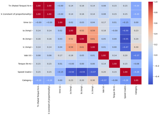
Figure 3.
Pearson correlation heatmap.
3.2.6. Feature Trends
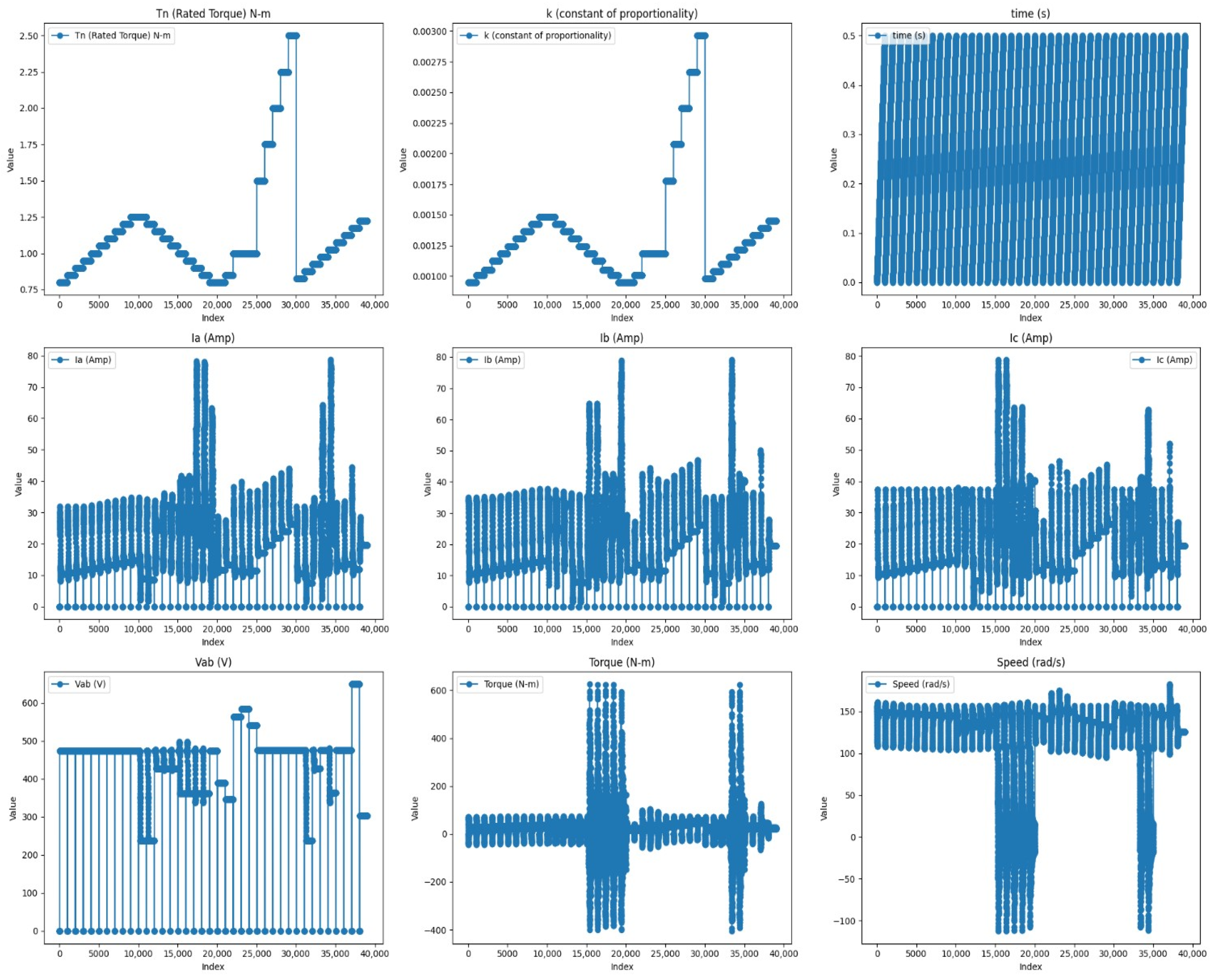
Figure 4 illustrates line plots, and it shows that the rated torque (Tn) and currents in phases A (Ia), B (Ib), and C (Ic) show high variability. The voltage between phases A and B (Vab) and speed also vary greatly. Also, each feature has many outliers. These may be due to changes in load, sensing errors, or mechanical issues. Among all the features, the time plot has constant value without variation, which there is a constant time interval for each measurement.
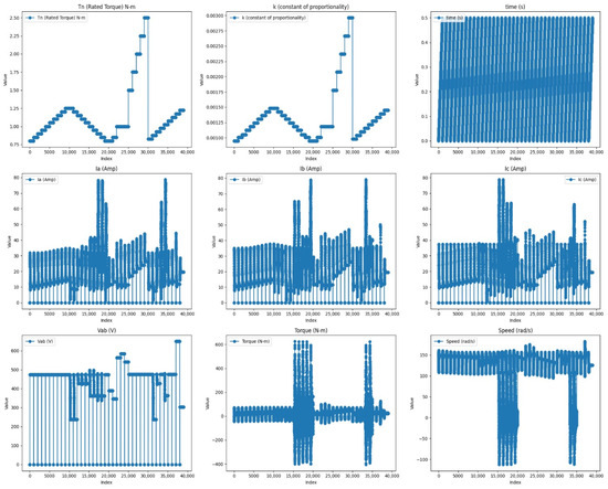
Figure 4.
Line plot of all features.
3.2.7. Feature Importance
The Random Forest feature importance [23] values in Figure 5 show that Vab, speed, k, and Tn are key features. On the other hand, time and torque hold less significance. This suggests they have a limited impact on fault detection results.
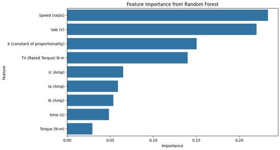
Figure 5.
Feature importance for Random Forest.
3.2.8. Analysis of Category Label Frequency
Figure 6 shows the category distribution in the dataset. NOM has the highest occurrences, while UVF has the lowest. The dataset shows a significant imbalance as NOM is a highly populated category, while PTPF and PTGF have the same number of entries.
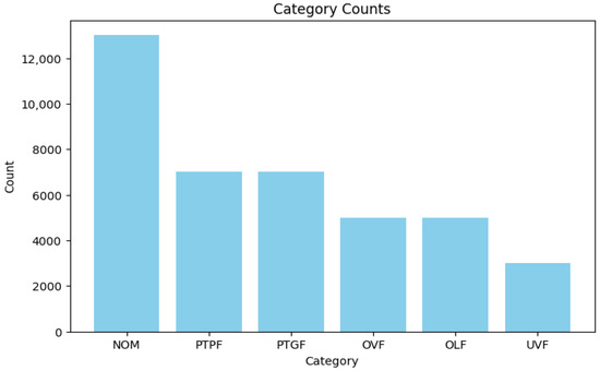
Figure 6.
Fault counts bar charts.
Figure 7 shows a pie chart. It displays the percentage breakdown of categories in the dataset. NOM has the highest percentage at 32.5%. In addition, PTGF and PTPF, respectively, make up 17.5%, OVF and OLF are each 12.5%, and UVF is 7.5%.
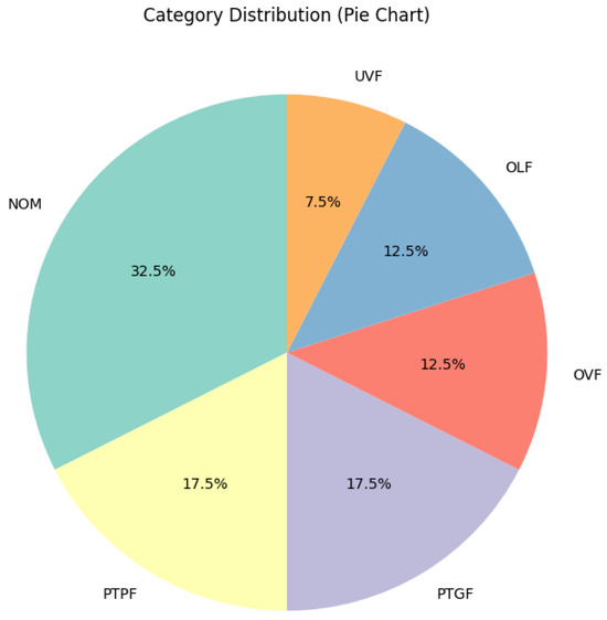
Figure 7.
Pie charts of fault.
3.3. Data Preprocessing
In machine learning tasks, data preprocessing is very essential [24]. Usually, raw data are incomplete, inconsistent, and noisy. Such issues can decrease the performance of a model. The purpose of preprocessing is to clean and organize the data. This indeed improves the analysis and consequently gives the model more precision and reliability.
The steps for preprocessing for classifying faults of electronic vehicle (EV) drive motors are given below.
3.3.1. Duplicate Row Handling
Duplicate data can negatively affect the performance of the model by creating bias and redundancy. For this study, we used Equation (1) to detect and handle duplicate rows. The use of this method led to the removal of 1000 duplicate entries from the dataset.
The following method detects and removes duplicate rows:
where the following is true:
- X represents the original dataset containing n rows.
- is an individual row in the dataset.
- D is the set of duplicate rows, where a row is considered a duplicate if it appears more than once in X.
- is the dataset after removing all rows in D (the duplicates).
- The operator represents the subtraction or removal of elements in D from dataset X, resulting in dataset .
3.3.2. Encoding Categorical Column
The ‘Category’ column in the dataset has six types of attack. For the transformation of these categorical values into numeric labels for machine learning, we use Label Encoding. The attack types get transformed into unique integer values that follow the pattern below:
By encoding the categorical data this way, it allows machine learning models to work with the categorical data in numeric format, that is required by most of the algorithms which cannot work with non-numeric values.
3.3.3. Outlier Detection and Removal
There are many outliers in the dataset, as can be seen from the exploratory data analysis (EDA) earlier. To overcome this situation, we detect and remove the outliers using the Interquartile Range (IQR) method [25]. The reason for choosing the IQR method is that features in the dataset are not normally distributed. By doing this, it becomes more robust than assuming normality.
Here is how the process works:
After detecting the outliers, rows containing them are filtered out:
3.3.4. Feature Significance
The feature significance was assessed through a one-way ANOVA test [26]. ANOVA tests show how features impact the target variable. They also identify which features are statistically significant.
Following analysis, the following decisions were made:
- We find that IC (Amp) is also insignificant and hence removed from the dataset.
- Time is important in statistical tests. However, we remove it for further analysis since faults do not depend on time.
Table 6 shows the one-way ANOVA results for each feature.
Table 6.
Feature significance results based on one-way ANOVA test.
3.4. Dataset Splitting
We split the dataset using an 80-20 ratio. This means 80% is for the training set, while 20% is for the testing set. After the split, we checked the category distribution in both sets. Table 7 shows the distribution of each category in each set.
Table 7.
Category distribution in training and testing sets.
3.5. Feature Selection
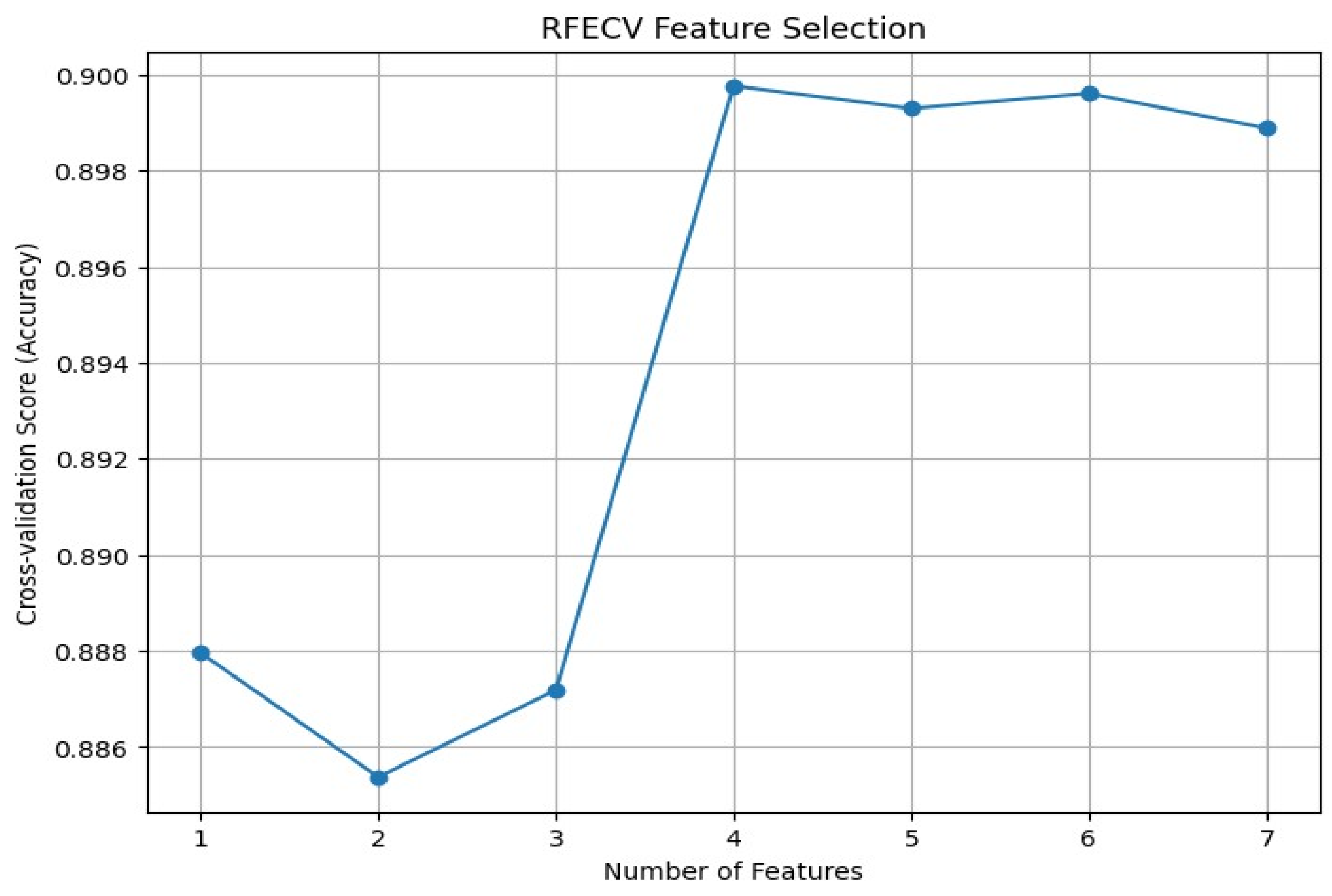
Feature selection is performed to make the model lighter and less time-intensive. We used the Recursive Feature Elimination with Cross-Validation (RFE-CV) method [27]. This feature selection process is conducted only on the training set to ensure that the features chosen are based on the training data, which prevents any data leakage into the testing set.
The highest cross-validation score of 89.98% is achieved using four selected features, which is why they were retained. The following Table 8 shows the scores of cross-validation for different numbers of selected features, which gives the evolution of performance when features are added.
Table 8.
Cross-validation scores for different models and selected features.
After feature selection, four out of the seven original features were used for further analysis. The final selected features are as follows:
- Tn (Rated Torque) N-m.
- Ia (Amp).
- Vab (V).
- Speed (rad/s).
In the following, Figure 8 shows the CV scores in feature-wise obtained during the feature selection process. Also, Algorithm 1 shows the steps of selecting features.
| Algorithm 1 Feature Selection using RFECV |
|

Figure 8.
Feature-wise cross-validation (CV) scores.
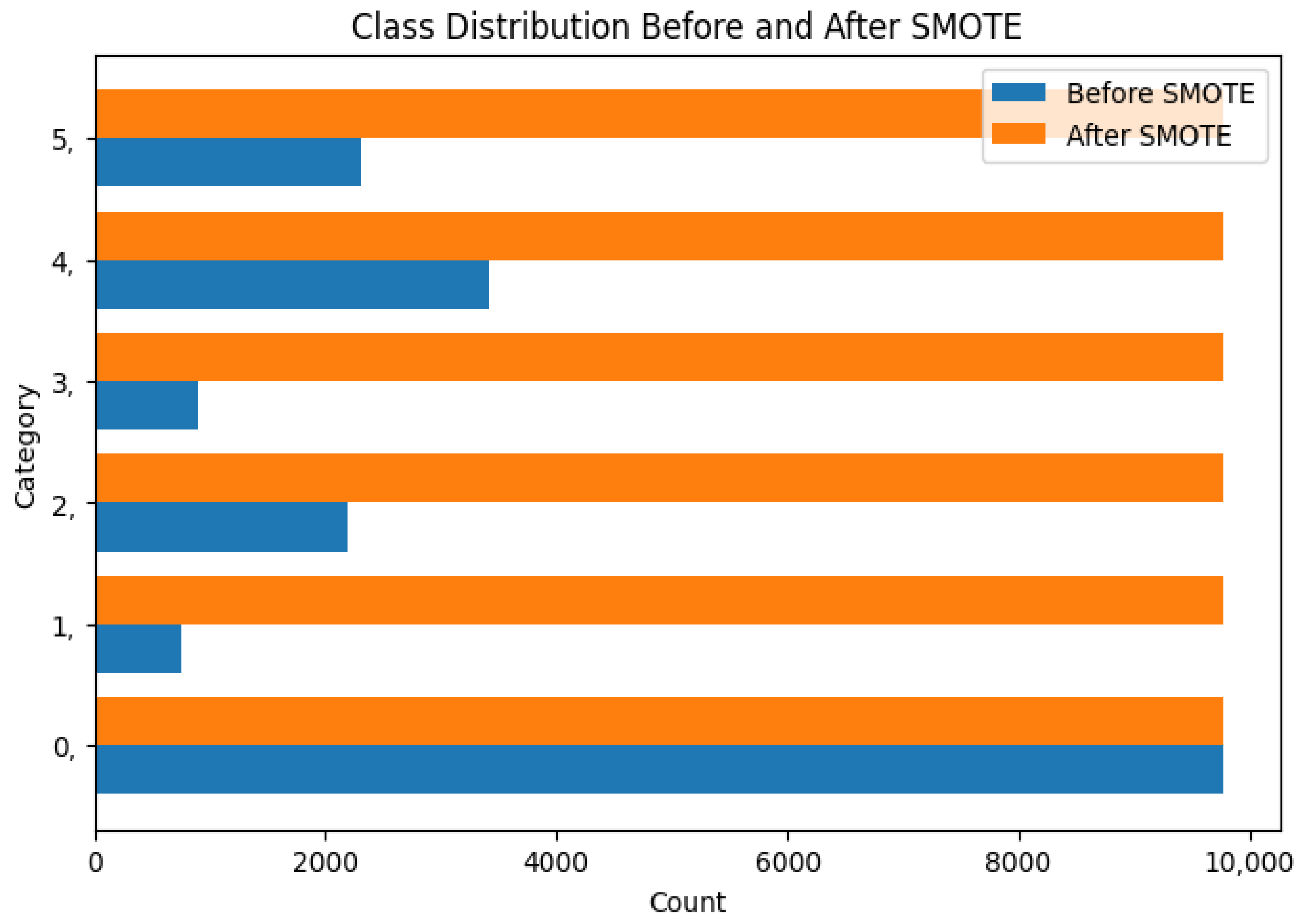
3.5.1. Data Balancing
When we split the dataset, Table 7 clearly showed that the training set has a record of a high class imbalance. This issue was overcome using the Synthetic Minority Over-sampling Technique (SMOTE) [28], and we used the model to improve model performance. We apply SMOTE and compare them in Figure 9.
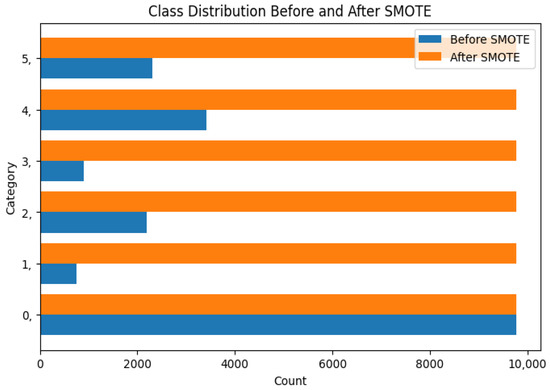
Figure 9.
Before and after balancing.
3.5.2. Standardization
Both the training and test sets were standardized such that each feature has a mean of 0 and a standard deviation of 1. This step is necessary to eliminate any scale-dependent bias and to improve the convergence and the hardiness of the model.
3.6. Model Training
Accurate classification of faults in electric vehicle drive motors is the key to maintaining vehicle performance and safety. For this experiment, eight different machine learning models were tested to determine which ones are effective in diagnosing the motor faults. The models evaluated include the following:
- Random Forest (RF): A type of ensemble learning that combines many Decision Trees using bagging in order to increase classification accuracy. The final prediction is made by voting on all of the trees in the forest.where the following is true:
- –
- is the final predicted class;
- –
- is the prediction from the ith Decision Tree;
- –
- n is the number of trees in the forest.
- Decision Tree (DT): A supervised learning model that splits the data into subsets based on feature values to classify motor faults.where the following is true:
- –
- is the predicted class;
- –
- is the set of possible classes;
- –
- is an indicator function that is 1 if the class label matches class c and 0 otherwise.
- Extra Trees (ET): An ensemble method that builds multiple Decision Trees similar to Random Forest but with a different randomization technique for splitting nodes.where the following is true:
- –
- is the final predicted class;
- –
- is the prediction from the ith Decision Tree;
- –
- n is the number of trees in the forest.
- K-Nearest Neighbors (KNN): A non-parametric classifier that assigns a class based on the majority class of the k-nearest data points.where the following is true:
- –
- is the predicted class;
- –
- are the classes of the k nearest neighbors;
- –
- k is the number of neighbors considered.
- Multilayer Perceptron (MLP): A type of neural network that learns to map input features to output labels by training multiple layers of neurons.where the following is true:
- –
- is the predicted output;
- –
- are the input features;
- –
- are the weights;
- –
- is the bias term;
- –
- is the activation function (e.g., ReLU, Sigmoid).
- CatBoost: A gradient boosting algorithm designed for categorical data that builds Decision Trees to minimize classification error.where the following is true:
- –
- is the final prediction for input ;
- –
- is the tth tree’s prediction;
- –
- is the learning rate for the tth tree;
- –
- is the total number of trees.
- XGBoost: An efficient gradient boosting algorithm that improves on Decision Trees using regularization and parallelization.where the following is true:
- –
- is the final prediction for input ;
- –
- is the tth tree’s prediction;
- –
- is the learning rate for the tth tree;
- –
- is the total number of trees;
- –
- is the regularization parameter for tree weights .
- Soft Voting Classifier: An ensemble method that combines the predictions of multiple models by averaging their probabilities and selecting the most probable class.where the following is true:
- –
- is the final predicted class;
- –
- is the predicted probability of class c for model i;
- –
- is the number of models in the ensemble.
3.7. Hyperparameter Settings
Hyperparameter tuning is essential to obtain maximum model performance. All the models in our research were initialized with certain hyperparameters to achieve optimal accuracy and efficiency. Table 9 below summarizes the most important hyperparameters used for every model.
Table 9.
Hyperparameters of the models used.
3.8. Cross-Validation
In order to evaluate how well the models perform for the whole dataset and to assess their generalization, we evaluated it by 5-fold cross-validation. The use of this method ensures that the models are not overfitted to a particular subset of the data during training and testing on different splits.
3.9. Explainable AI
Finally, LIME (Local Interpretable Model-Agnostic Explanations) [29] was applied to the proposed model in order to use this model in a transparent manner so that it can be understood how the predictions are made. LIME introduces local interpretations through an approximation of a complex model with simpler ones; hence, they can identify the factors that influence the classification decisions.
Below, Figure 10 shows the overall workflow diagram for efficient EV motor fault classification.
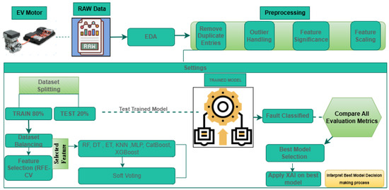
Figure 10.
Proposed approach for electric drive motors fault classification.
4. Results and Discussion
In this section, we provide training and testing results to evaluate the machine learning model in detecting faults of Electric Vehicle (EV) drive motors. Finally, the results are analyzed using evaluation metrics described in Table 10. To evaluate the machine learning models we used to classify the fault in the electric vehicle drive motors, different metrics are used. The metrics let us know how accurate, reliable, and generally valid the model is. Table 10 describes the key evaluation metrics, their definition, and the equations of the model performance.
Table 10.
Evaluation metrics with descriptions and formulas.
4.1. Experiment 1: Drive End Simulated Dataset
4.1.1. Training and Validation Performance
Table 11 shows the performance of several machine learning models, including Random Forest, Decision Tree, Extra Trees, K-Nearest Neighbors (KNN), Multi-Layer Perceptron (MLP), CatBoost, XGBoost, and Voting Classifier, evaluated with respect to training accuracy, mean cross-validation (CV) accuracy, and standard deviation.
Table 11.
Training accuracy and cross-validation scores.
First of all, XGBoost achieved the highest training accuracy of 98.45 percent, a mean CV accuracy of 97.19%, and the lowest standard deviation of 0.0006, which proves its high consistency in training tasks through various training sets. Upon doing the same, CatBoost tied behind the first runner at 97.96% training accuracy, 97.05% mean CV accuracy, and 0.0031 standard deviation, largely behaving stably but more variably. Also, the Voting Classifier had a training accuracy of 97.82%, and we achieved a mean CV accuracy of 97.10% and a standard deviation of 0.0012, which is a relatively high stability and proves to be a reliable generalization. Moreover, the Random Forest had a training accuracy of 97.40%. It also achieved a mean CV accuracy of 96.55 and a low variance of 0.0021, showing a solid performance. The Decision Tree model achieved a training accuracy of 96.17%. Its mean CV accuracy was 95.36%, with a standard deviation of 0.0031. The Extra Trees were trained to 95.25% accuracy, the mean CV accuracy was 95.06%, and the standard deviation was 0.0045; thus, they showed higher variability in performance from run to run. In particular, KNN and MLP, with their training accuracies of 96.58 and 94.70%, respectively, exhibited higher fluctuation in their performance with higher standard deviations. To conclude, XGBoost and CatBoost serve as the most reliable models, but XGBoost is the most stable one in terms of the evaluation provided in Table 11. The Voting Classifier also performed very well and was quite consistent. Random Forest, Extra Trees, KNN, and MLP had greater variability. Still, their accuracy was quite competitive.
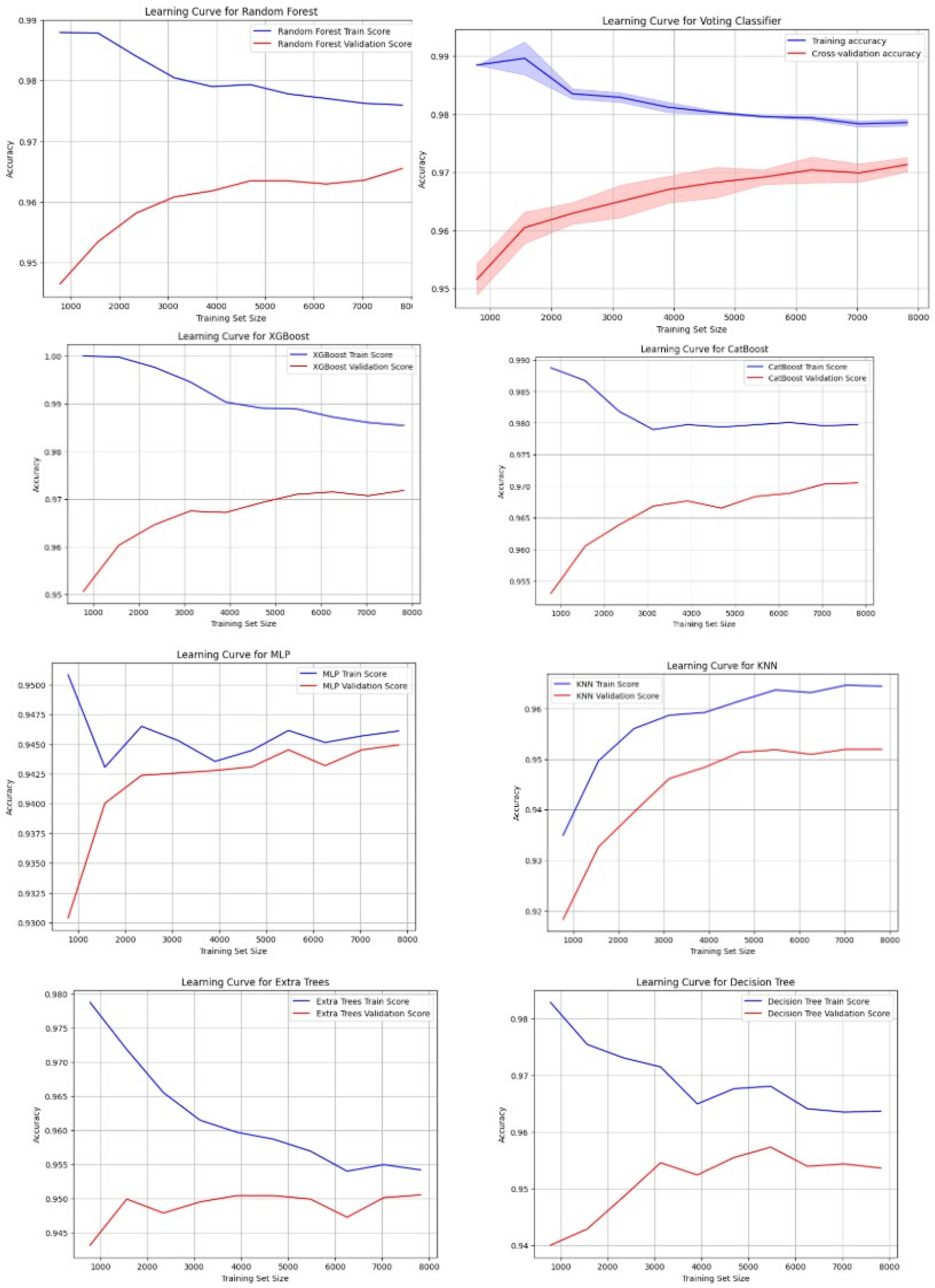
Next, the learning curves of the models are added in Figure 11. In addition to this, it helps us understand how the models learn over time, and these curves provide additional insight into how their training behaves, evolves with their performance, and how they may even be headed for overfitting or underfitting.
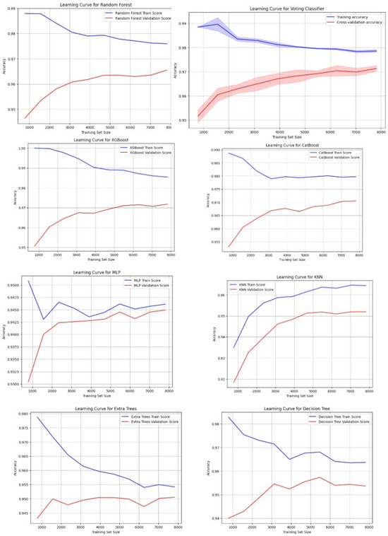
Figure 11.
Learning curve of all models.
As shown in Figure 11, XGBoost, CatBoost, and Soft Voting were the most consistent curves because both training and validation accuracy curves rise upward, indicating that they improve in a steady manner during both training and validation. They generalize well between training and validation times. The second is Random Forest, which is close behind with good learning and little overfitting. KNN and MLP perform similarly. Both models are slightly overfitted as they show more variability in validation accuracy. However, the gap between training and validation accuracy is small. Random Forest performs well, too, but it is slightly overfitted more than Extra Trees. Although the Decision Tree model does well on training data, it heavily suffers from overfitting as the model performs poorly on validation data. To know the computational cost of each model, we summarize the training time, memory usage, and inference time of each model in Table 12.
Table 12.
Model training times, memory usage, and inference time.
Training times are shown in Table 12, and the Decision Tree is the fastest of them all being 0.0394 s. KNN and Extra Trees also show quick training times of 0.0119 s and 0.6435 s, respectively, with Extra Trees maintaining a good balance between performance and computational cost. Comparatively, CatBoost and XGBoost have very fast training times of 5.20 and 0.6401 s, respectively, whereas MLP needs a vast amount of time (33.72) s. The Voting Classifier, with a training time of 23.64 s, shows competitive performance but with higher computational costs.
All the models have relatively low memory usage in terms of memory used, with the minimum memory populated by the Voting Classifier (0.00 MiB). Similar to that, inference times are primarily low across the board, with Voting Classifier having the highest inference time of 0.3955 s, which is quite efficient. In fact, other models such as KNN (0.7607 s) and XGBoost (0.0642 s) also take inference times that are shorter than other models tested, which shows that all the models are able to provide quick results even on bigger datasets.
4.1.2. Testing Performance
The testing results presented in Table 13 demonstrate that XGBoost obtained 94.35% accuracy along with a 0.9964 AUC score. Moreover, CatBoost performed slightly better with 94.50% accuracy and an AUC score of 0.9965. Random Forest showed similar effectiveness to other classification methods and achieved an accuracy of 94.39% and an AUC score of 0.9958. Also, Decision Tree obtained accuracy results of 94.02% with an AUC score of 0.9927. The accuracy and AUC performance of Extra Trees reached 93.25% and 0.9934, respectively. The performance accuracy for KNN and MLP stood at 92.09%, alongside 92.12% for accuracy and AUC scores of 0.9877 and 0.9942.
Table 13.
Model Accuracy and AUC Scores.
A Voting Classifier is an ensemble model that predicts the output based on the prediction of multiple models. With this approach, the performance achieved 94.52% accuracy and an AUC of 0.9960. The results of the test showed that each model is performing well; hence they can generalize to unseen data too. Compared with the other models, the Voting Classifier performed slightly better as it yields the output based on the predictions of other models. In addition, we evaluated the models based on precision, recall, and F1 score, which are in Table 14. These metrics provide essential information about model instance classification accuracy together with precision–recall equilibrium, which strengthens fault classification evaluation.
Table 14.
Precision, recall, and F1 score for different models and classes.
The precision, recall, and F1 scores for all the models evaluated in six classes are shown in Table 14. All models for class 1 and class 2 have shown perfect performance, scoring 1.0000, which means that they are performing extremely well for those classes. Moreover, Random Forest, Extra Trees, and Voting Classifier perform well in class 0 with F1 scores between 0.93 and 0.94, and KNN has a slightly lower F1 score than others. In addition, for the models that do well in class 3, F1 scores are approximately 0–0.75 (CatBoost, XGBoost, and Voting Classifier), and the worst-performing model is KNN, with the lowest F1 score. Random Forest, CatBoost, and Voting Classifier score more than 0.90 F1 score in class 4, which is substantial. Finally, the Voting Classifier and XGBoost reach almost perfect F1 scores for class 5. In general, the Voting Classifier and CatBoost models yield a balanced and reliable performance on all classes, with stable precision, recall, and F1 scores. Further, for better understanding, below are included the confusion matrix, ROC curve, and precision–recall curve, which provide insights about the models performed in different ways of examining.
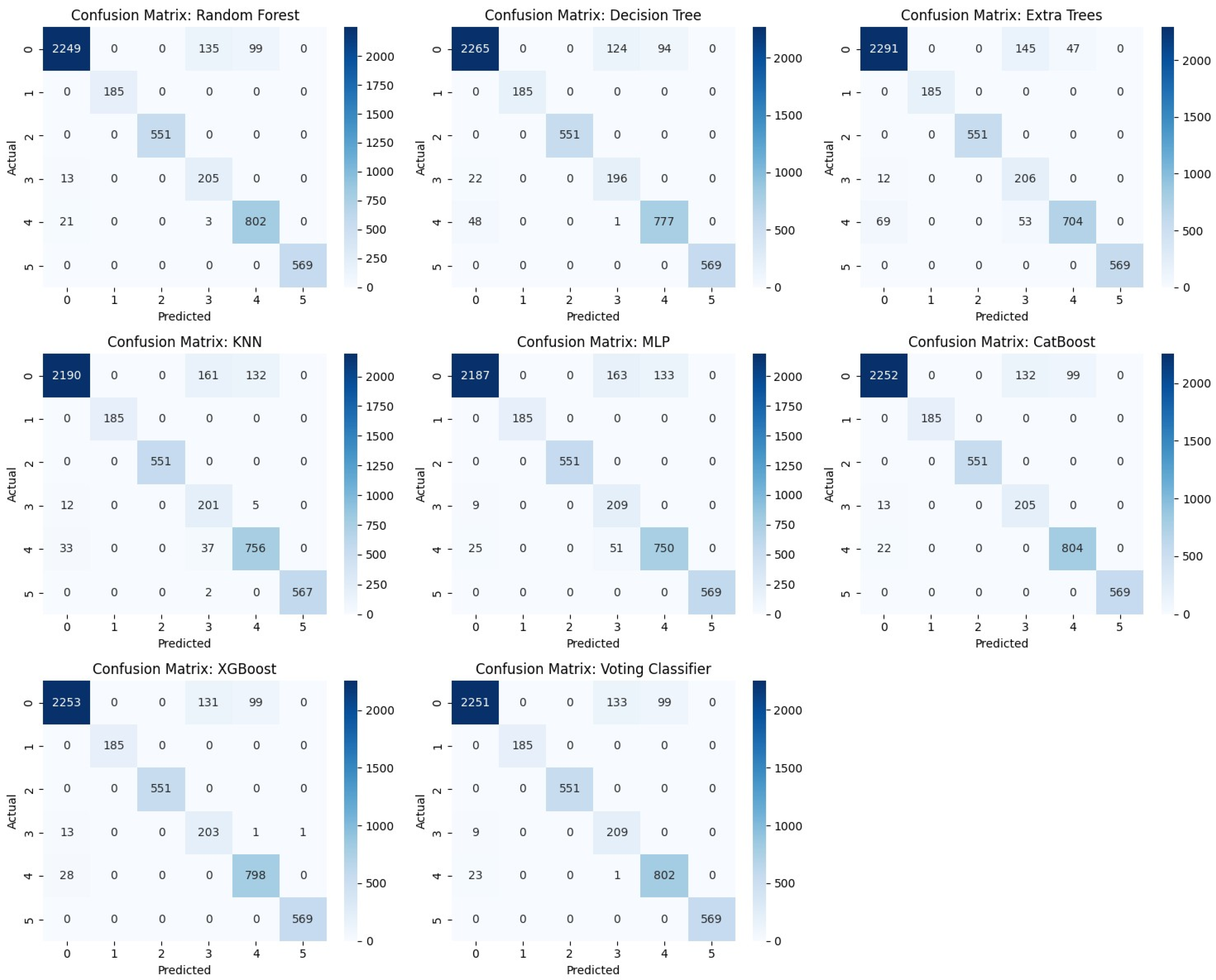
As shown in Figure 12, the confusion matrix of each model is presented, which makes it easier to compare the performance of each model. The matrix shows how well each model classifies positive and negative samples as TP, TN, FP, and FN. TP and TN values of the models such as CatBoost, RF, and XGBoost are high, which means that the models are very well performing. Unlike the Decision Trees and KNN, there are slightly higher FP and FN values. The Voting Classifier balances the classification errors slightly better than the others, with fewer misclassifications. Overall, the models RF, CatBoost, and XGBoost outperformed the other models, while the Voting Classifier was able to improve performance slightly.
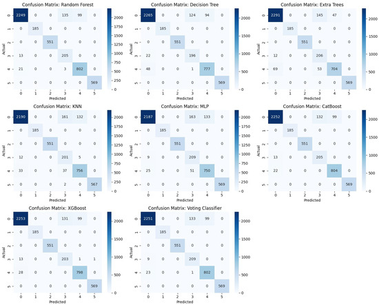
Figure 12.
Confusion Matrix.
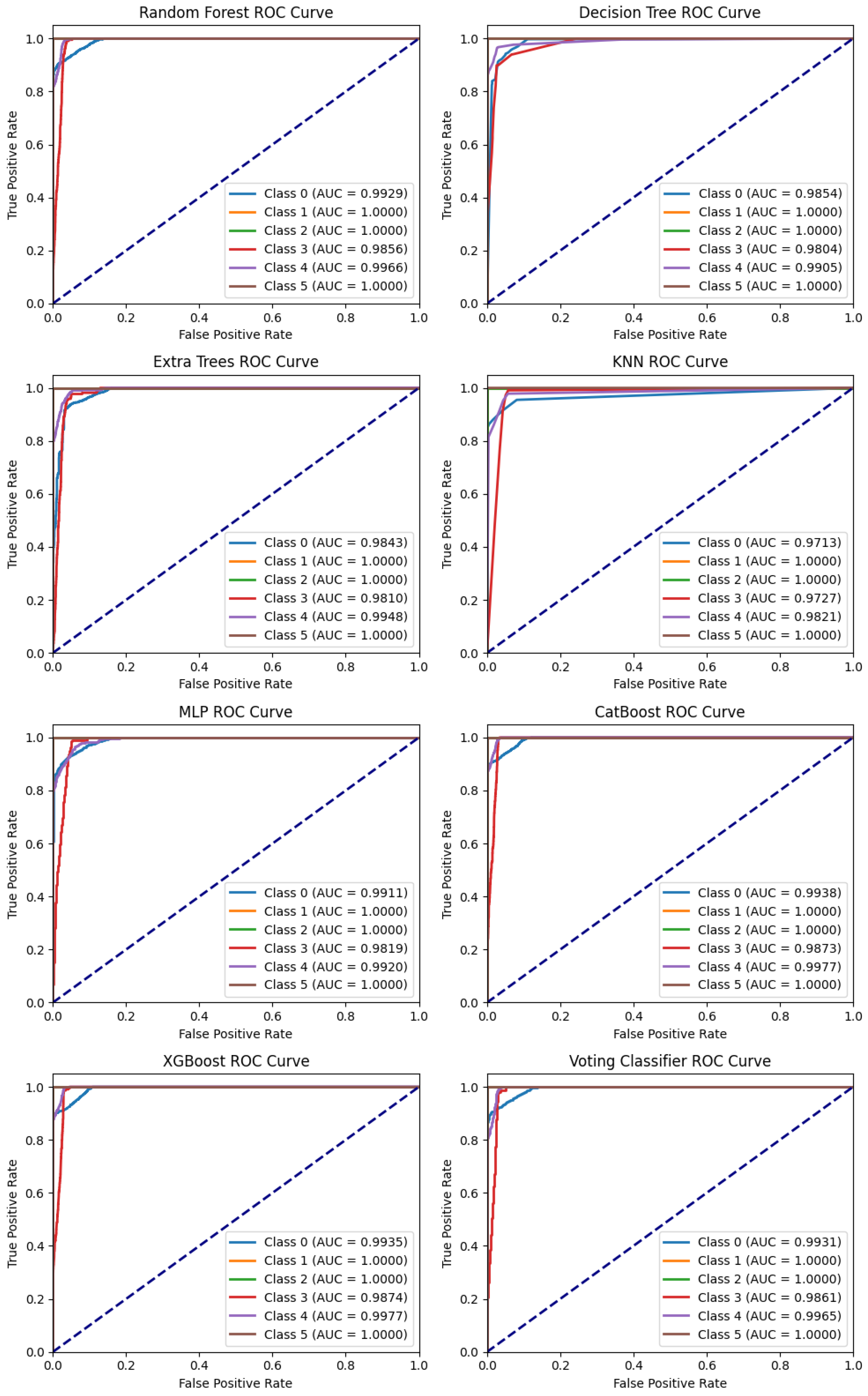
Figure 13 shows that most models show strong ROC curves for all classes. However, class 3 is an exception. All models struggle to make accurate predictions for this class. The top performers overall, including class 3, are XGBoost, CatBoost, and the Ensemble Soft Voting Classifier.
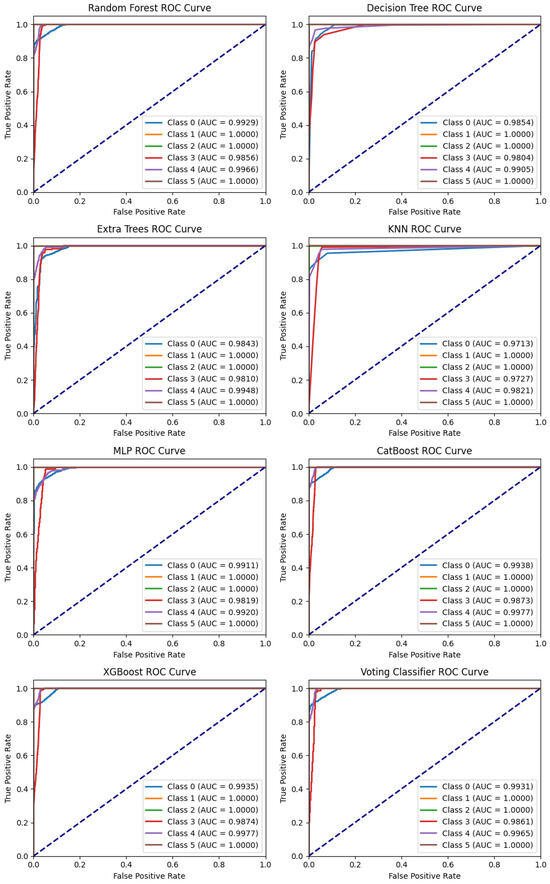
Figure 13.
ROC curve of all model.
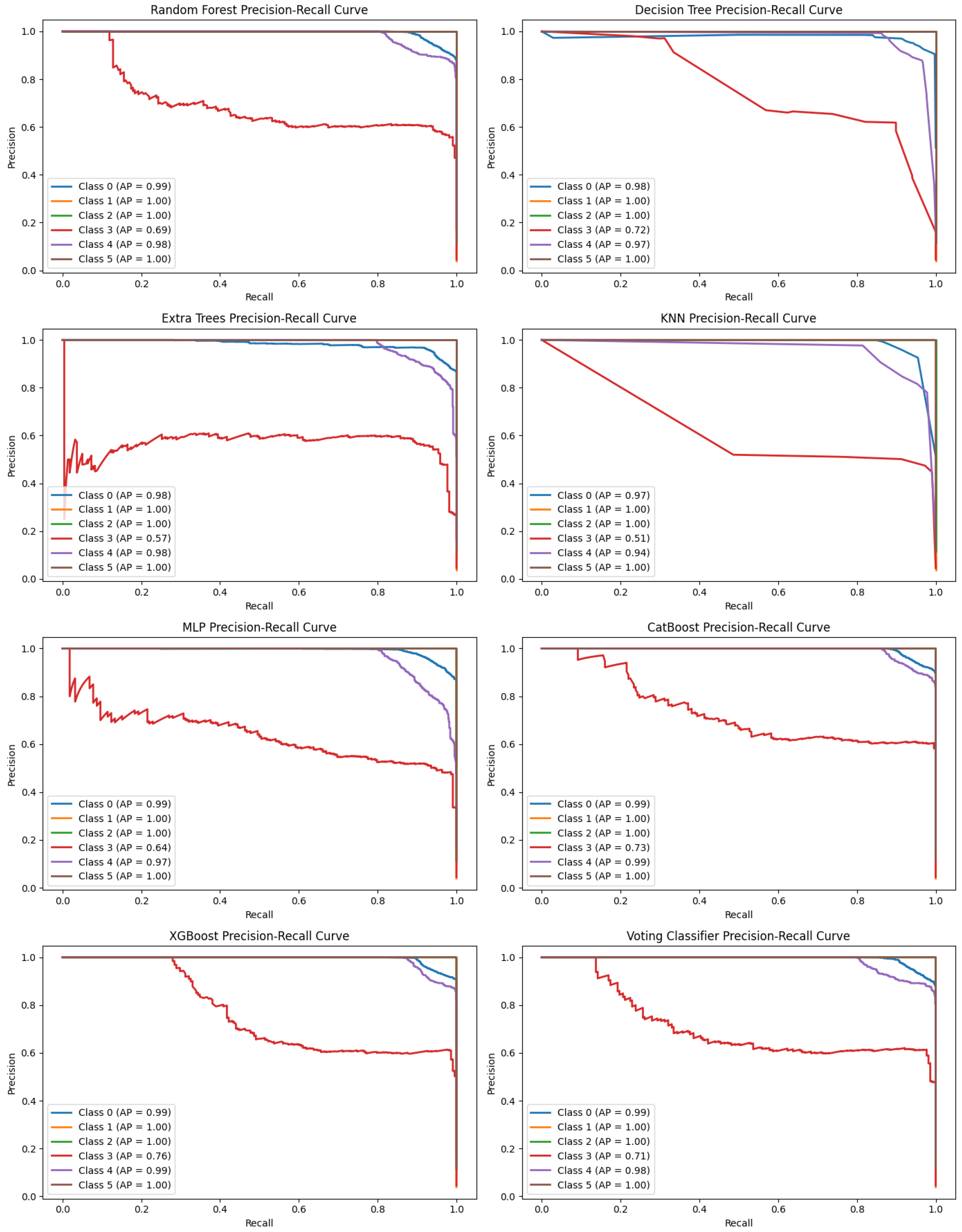
In multiclass classification, precision–recall curves are important because they evaluate model performance under imbalanced data situations. While the ROC curve deals with overall discrimination, PR curves actually show how well one trades off between precision (minimizing false positives) and recall (minimizing false negatives) for each one of the classes.
In Figure 14, it can be said that XGBoost, CatBoost, Extra Trees, and Random Forest have higher values for average precision, thus showing good performance for multiclassification. The Voting Classifier got some improvement in terms of precision and recall from ensembling. However, the KNN and Decision Tree are more variable and seem to have issues with certain classes, especially in terms of being imbalanced.
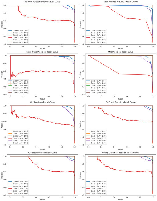
Figure 14.
Precision–recall curve of all model.
4.1.3. Assessing Model Reliability with Kappa
It is critical to measure the agreement of the true labels with the models’ performance for various machine learning models to fault classification in the electric vehicle drive motors (EVDMs). Cohen’s Kappa is one of those and is helpful in a robust evaluation rather than accuracy alone. Kappa scores help us understand the consistency or reliability of classifiers in reality.
Table 15 shows that the Voting Classifier with a result of 0.9210 is the most consistent and agrees most with true labels, making it the most deterministic model to be used for fault classification. Random Forest, with a score of 0.9192; CatBoost, with a score of 0.9206; and XGBoost, with a score of 0.9184, all do extremely well on their models with Kappa scores close to 1, meaning good classification performance and a little bit of random agreement. The Decision Tree, with a score of 0.9133, and Extra Trees, with a score of 0.9021, while slightly lower, still exhibit high reliability and consistency in their predictions. On the other hand, KNN, with a score of 0.8869, and MLP, with a score of 0.8874, were the least consistent and had the highest chance of random agreement to fault classes.
Table 15.
Cohen’s Kappa Scores.
4.1.4. Best Model for Fault Classification in Electric Vehicle Drive Motors
Based on the analysis of training accuracy, cross-validation accuracy, training time, memory usage, inference latency, testing score, Kappa score, AUC, ROC curve, precision–recall curve, and confusion matrix of all other models used in the experiment, it is concluded that the ensemble soft voting model is the most consistent model for fault classification in electric vehicle drive motors. In terms of these key metrics, the soft voting model performed consistently and outperformed other models in generalization effectiveness and in providing reliable results. In addition, the model only took 23 s to train, which made the model highly efficient. Although it is an ensemble model, it had a reasonable memory usage of 0.00 MiB with an inference time of 0.3711 s, which allowed real-time predictions to be made. The ensemble soft voting model is demonstrated to be the best for this task in terms of its performance on all evaluation criteria and computational efficiency.
Below is Table 16 of metrics of the soft voting model.
Table 16.
Metrics of the soft voting model.
4.1.5. Interpreting the Best Model’s Decisions with XAI
We applied LIME (Local Interpretable Model-agnostic Explanations) to our best-performing ensemble soft voting model to analyze its decision-making process. LIME allowed us to examine the model’s predictions for each of the six classes in the dataset. For every class, we observed how the model assigns predictions and interpreted the importance of various features that contributed to those predictions. This detailed analysis provided us with insight into the behavior of the ensemble model, demonstrating how it approaches each class and ensuring consistent and reliable classification across the entire problem set. The interpretability of these predictions for each class is outlined below.
As can be seen in Figure 15, the LIME XAI explanation of class 0 at index one clearly states that the model is very sure that the instance will belong to class 0, and this is with 91% certainty. This decision is mainly driven by rated torque, which in this case is contributing the most, suggesting that the lower torque value is of great importance so the model tends to shift towards class 1 less. Furthermore, the speed and current support the prediction for class 0, though the influence is less. The voltage itself has a minor impact on class 1, alongside the other features. However, this proves that the main factors, such as rated torque, lead to the prediction converted towards class 0 with high confidence. To conclude, all the features combine to make the predictions of the model, and a combination of negative features outweighs positive features, thus giving a final class of 0.
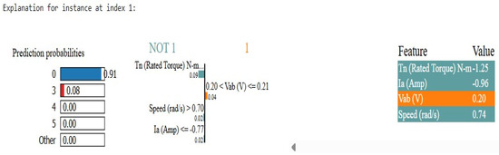
Figure 15.
LIME Explanation for prediction class 0.
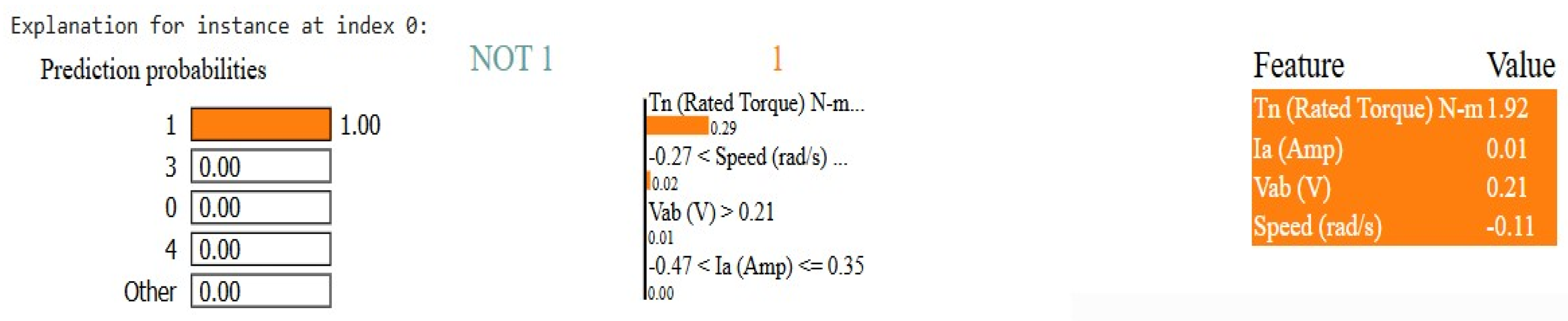
Figure 16 shows the LIME explanation of class 1 at index 0 in Figure 16, where the model is 100 percent confident that this is the prediction for class 1. The most significant positive contribution to this classification is Rated Torque Tn equal to 1.92. Voltage Vab, Current In, and Speed also influence the prediction but to a lesser extent. Finally, the model’s reasoning process indicates that a high-rated torque would immediately lead to class 1 and does not ask for additional evaluation of other features. This implies that torque is an important contributor to classification and other features have a secondary contribution to this classifier.
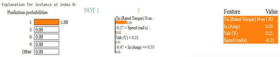
Figure 16.
LIME Explanation for prediction 1.
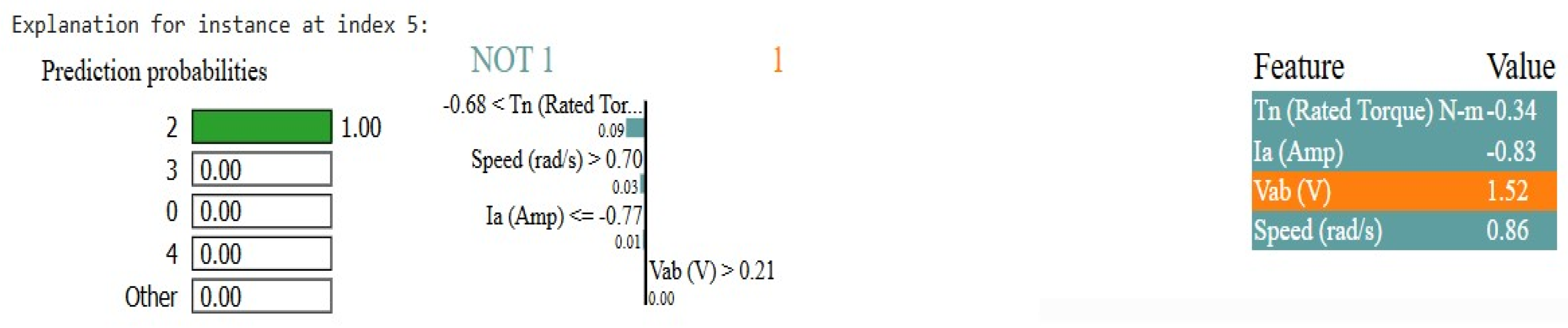
The LIME explanation for class 2 at index 5 in Figure 17 indicates that the model is 100% sure that the instance should be of class 2. The main reason this is the case is because of the speed value, which ranges from typical class 2 of 0.86. This also supports the rated torque of −0.34, which is in class 2 because lower torque values are common in this class. Subsequently, the current of −0.83 cannot be related to the condition required for class 1, and hence, class 1 is also rejected. Looking at the voltage of 1.52 pointing to class 2 as well as 0.21 points to class 2. Overall, these values are good characteristics for the model in predicting class 2, with speed, torque, current, and voltage all being important for such a decision.
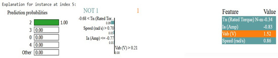
Figure 17.
LIME Explanation for prediction 2.
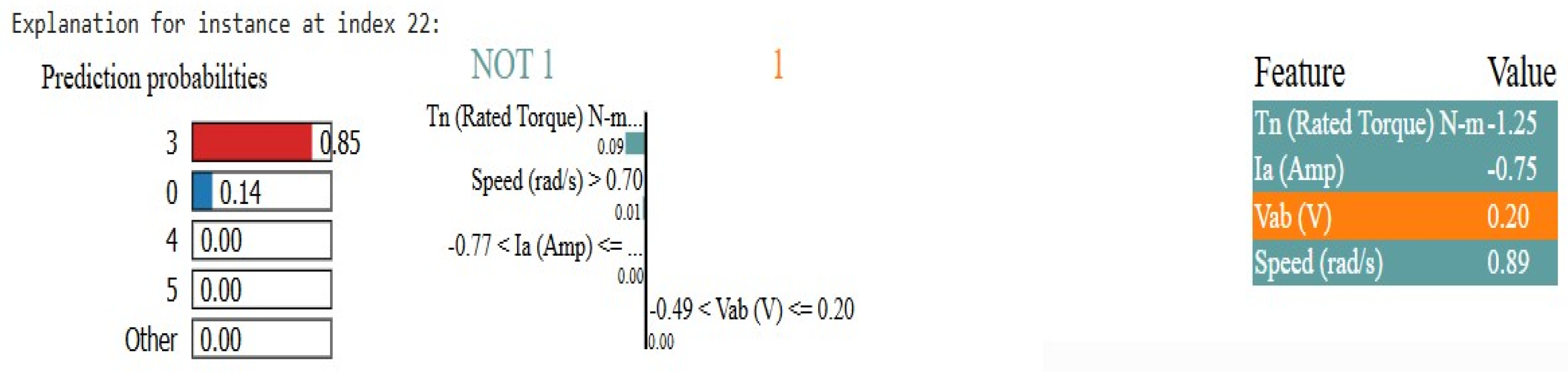
In Figure 18, it is shown that the model predicted class 3, for instance, 22, with 85% confidence. The reason for this prediction is a high-rated torque, supporting class 3. This decision also depends on speed, however, not as much. As the current and voltage slightly push the prediction away from class 3, they have a slight negative impact. Even so, rated torque and speed have a much stronger effect than this result. This model has predicted a class of 0 with a 14% probability and all other classes with a probability of 0. It’s the best match for this instance and doesn’t fit into other classes; as such, this confirms that class 3 is the correct one. Figure 4 illustrates overall that the model is able to classify an instance as class 3 when rating torque and speed are high and a small effect of voltage and current.
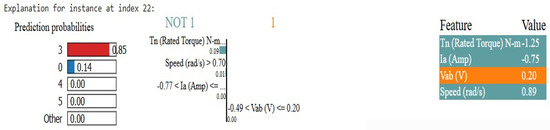
Figure 18.
LIME Explanation for prediction 3.
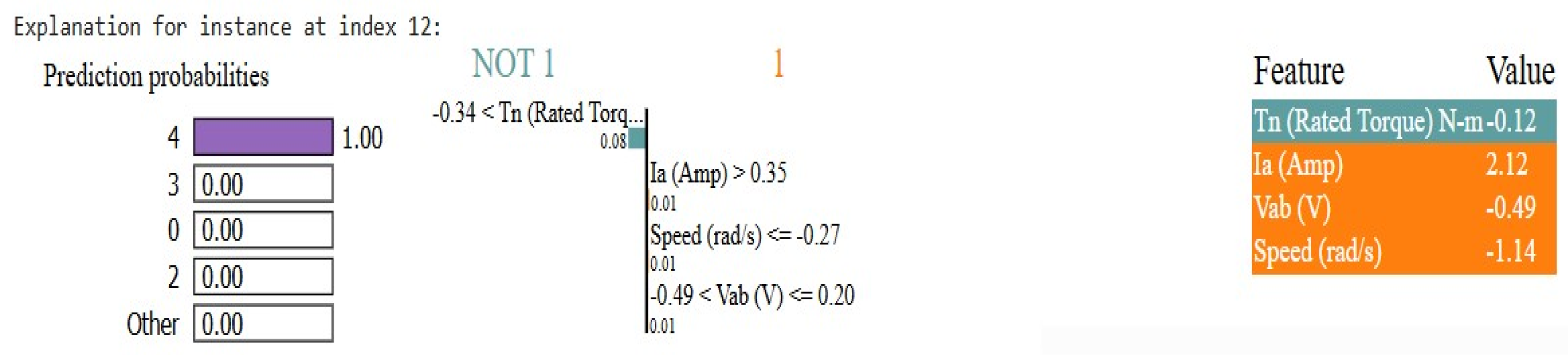
Figure 19, it shows the model predicts class 4 with 100% confidence for index 12. This decision is mainly based on the low-rated torque (−0.12), as this supports class 4. Not only that, speed (−1.14) also plays a crucial role, as its negative value also fits the pattern of class 4. Another reason the model selects class 4 is that 2.12 > 0.35, which is current (Ia). This is classified as voltage (Vab) is −0.49, which is within some given range that also verifies this classification. Since the probabilities of all other classes are 0%, the model can rule them out completely. Figure 5, overall, indicates this as being class 4 with absolute certainty through low-rated torque, low speed, high current, and specific voltage.
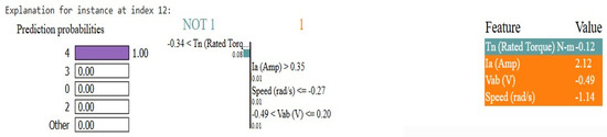
Figure 19.
LIME Explanation for prediction 4.
In Figure 20, we see that instance 2 has 100% confidence of being decided as class 5 by the model. So in other words, this result is sure that this instance is of class 5 and has no other possible prediction. Given the rated torque value of −1.25, this prediction is the most important number and clearly supports class 5. This is also a factor that contributes to this classification at the voltage (Vab) of −1.06. This smaller positive contribution is given by the current (Ia) of −0.77. The model’s decision is relatively speedless (0.25), having little (or no) effect on whether the instance is from class 5. The model rules out all other classes since their probabilities are 0%. Figure 6 shows overall that for this instance—specifically for values of rated torque and specific voltage and current values that are low along a neutral speed—the combination of all of these values confirms this was class 5 with absolute certainty.
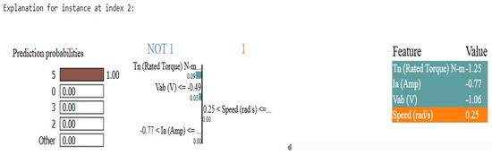
Figure 20.
LIME Explanation for prediction 5.
4.2. Experiment 2: Drive End Experimental Dataset
Experiment 1 was conducted previously on a MATLAB-simulated dataset. In this experiment, a dataset from Zenodo is used with a total of nine classes to further validate the framework’s effectiveness. The data preparation, model training, evaluation, and performance comparison in this experiment are exactly the same as in Experiment 1, so there will be no dependency on the randomness of these steps applied.
Table 17, various machine learning models are compared in terms of training accuracy, cross-validation accuracy, training time, inference time, and memory usage. The training result demonstrates that XGBoost has the highest training accuracy of 99.94% and a cross-validation of 99.45%, which shows it has strong generalization performance. Furthermore, trained with the Voting Classifier, which consists of several models, the system achieves high accuracy, achieving 99.79% in training and 99.40% in cross-validation. However, this compromises the training time, which is much higher at 103.94 s and has the highest memory usage of 2.64 MB. CatBoost and Random Forest also exhibit competitive performance, reach high estimation accuracy, and train fairly well, which makes them natural deployment candidates.
Table 17.
Comparison of model performance metrics.
Models such as Decision Tree and Extra Trees achieve great accuracy, but their generalization performance is not so good as ensemble model-based models. KNN is the slowest, as 3.56 s is its longest inference time, and it might experience issues with real-time applications (despite the training phase being fast). The deep learning-based approach used with MLP helps balance the accuracy and adequacy in computation time, but it has a higher training time than traditional machine learning models.
Results from this experiment suggest that the proposed framework works well on different datasets and has robustness in multi-class classification problems. Further strengthening the validity of the approach is the transition from a simulated dataset to a real-world dataset with nine classes as the first transition from a simulated dataset to a real-world dataset with scenarios. Since the framework has been proven to work on Experiment 1, the consistency of the framework remains the same, allowing it to work similarly on various datasets.
Table 18 also presents the testing consistency report that confirms the training of models using the provided data is indeed reliable by testing it on unseen data. Finally, results justify the applicability of the framework in a real-world scenario.
Table 18.
Model performance on test set.
The model performance metrics on the test set are presented in Table 18, which offers a strong evaluation of the models’ ability to generalize to unseen data. The accuracy, AUC score, testing time, and Kappa score, which measures the agreement between predicted and real classification adjusting for chance level accuracy, are the key metrics of this.
It can be seen from the table that XGBoost has the highest accuracy (98.71%) and AUC score (0.9997), which is very good for discriminating between classes in the data. On the other hand, the Voting Classifier, which is created by combining several models, has the highest Kappa Score (0.9976), indicating a very good agreement between the predicted and actual class labels, and therefore has the best overall consistency. The test performance of Random Forest and CatBoost also shows good results with accuracy values of 98.67% and 98.62%, respectively, and high kappa scores.
The Decision Tree performs slightly lower than the ensemble models, but the testing time of 0.0049 s is quite low, and thus it is a good choice for real-time applications. On the contrary, although KNN achieves an accuracy of 96.41%, a testing time of 0.3040 s is the highest among all algorithms, which can be a bottleneck for time-critical prediction. Deep learning powers MLP to maintain a balance between Kappa Score and inference efficiency, achieving 0.9724 and having a small testing time.
Overall, the Voting Classifier as well as XGBoost, CatBoost, and Random Forest provide high predictive power as well as robustness. Most Kappa Scores are high across all models, which further reinforces the same reliability and stability of the proposed framework applied to a multi-class classification problem. Consistency between datasets validates the framework’s adaptability and the applicability of it to real-world scenarios.
We further add the Confusion Matrix, ROC curve, and precision–recall curve in Figure 21 to have a clearer look at the XGBoost model’s performance.
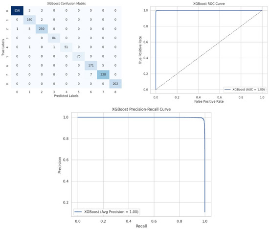
Figure 21.
Confusion Matrix, ROC curve, and precision–recall curve.
Figure 21 shows that XGBoost has a few misclassifications, whose ROC and precision–recall curves remain good, which indicates strong classification ability.
Finally, on the experimental data, XGBoost proved to be the best model after evaluating all performance metrics. It has a near-perfect (98.71%) accuracy, AUC score, and kappa score, ensuring strong predictive and consistent power. It also provides reasonable training (2.17 s) and inference (0.2815 s) times with minimal memory usage. Moreover, its high training accuracy (99.94%) and validation accuracy (99.45%) show how reliable this model is for this task.
4.3. Comparative Analysis with Previous Studies
We performed fault classification on an electric vehicle (EV) motor using a MATLAB simulated dataset for a fault classification. Thus, we compare our study to other studies that used simulated datasets for fault classification. Comparisons to these are used to determine what level of effectiveness our method offers in terms of prior studies.
A comparative analysis and key performance metrics of prior studies, including such parameters as accuracy, characteristics of the dataset, and classification techniques used in prior studies, have been presented in Table 19. Thus, it facilitates clear evaluation of variations and improvements of methodologies.
Table 19.
Comparison of fault classification studies on electric vehicle motors.
This Table 19 provides a comparison of the fault classification studies in the domain of electric vehicle motors. In our research, we employ the same simulated dataset that has been used by [8]. Our study surpasses this result, having an accuracy of 94.52%, while their study accuracy is 94.1%. We surpass the method described by [12], which used a comparable dataset to ours in all aspects of performance. Our Soft Voting Ensemble model stands apart from previous works since it delivers better performance results. The study incorporates Explainable AI (XAI) techniques to make the model more understandable while performing predictive maintenance operations. Lastly, to validate our findings, we also validate the model on another dataset, and we observe the robustness and effectiveness of our approach. Such an ensemble of methods, along with XAI, offers an approachable and transparent alternative to previous work in this area and achieves better accuracy and consistency.
5. Conclusions
In this study, we developed the EnsembleXAI-Motor framework for lightweight and efficient classification of faults in electric vehicle drive motors. With such techniques as statistical analysis, preprocessing, recursive feature elimination with cross-validation (RFE-CV), model tuning, and the hybrid soft voting classifier, we successfully obtained a test accuracy of 94.52% with a Kappa score of 0.9210. Local Interpretable Model-Agnostic Explanations (LIME) were incorporated to make the model’s decision-making process more transparent, thus making it very applicable for real-world applications where understanding the model’s predictions is necessary. In addition, the framework has low inference time and invokes tiny memory usage, which allows it to be used in real-time applications. In addition, we validated the performance of our framework using another real-world dataset and found that it had consistent performance, and thus it validated the robustness and generalizability of our framework across different conditions. The validation we have performed on the proposed framework further validates it as effective also in a real-world dataset, not only in a simulated dataset.
Our proposed framework not only improves diagnostic performance but also solves the problems of computational efficiency and model interpretability. In the fast-changing electric vehicle sector, there is a great need to detect faults timely and accurately, which is particularly important for improving safety and reliability.
Lastly, future work will focus on deploying the model on vehicle control units or IoT-based monitoring systems for real-time fault detection. Also, deep learning model integration will increase the accuracy, and continuous and transfer learning will boost adaptability to different motor types and fault patterns. Such advancements will facilitate scalability to large datasets and wider adoption to a larger range of motor systems.
Author Contributions
Conceptualization, M.E.H., M.Z. and J.U.; methodology, M.E.H., M.Z. and J.U.; software, M.E.H. and M.Z.; validation, M.E.H., M.Z. and J.U.; formal analysis, M.Z. and J.U.; investigation, M.E.H. and M.Z.; resources, J.U.; data curation, M.E.H. and J.U.; writing—original draft preparation, M.E.H.; writing—review and editing, M.E.H., M.Z. and J.U.; visualization, M.E.H. and M.Z.; supervision, J.U.; project administration, M.Z.; funding acquisition, J.U. All authors have read and agreed to the published version of the manuscript.
Funding
This research is funded by Woosong University Academic Research 2025.
Data Availability Statement
The data supporting the findings of this study are available in the repository for the experiment “Machine Learning-Based Fault Diagnosis of Electric Drives” at https://github.com/HassanMahmoodKhan/Machine-Learning-Based-Fault-Diagnosis-of-Electric-Drives/tree/main/Data (accessed on: 17 February 2025). Additionally, the experimental dataset can be accessed at https://zenodo.org/records/14482932 (6 April 2025).
Conflicts of Interest
The authors declare no conflict of interest.
Abbreviations
The following abbreviations are used in this manuscript:
| KNN | K-Nearest Neighbors |
| MLP | Multi-Layer Perceptron |
| ET | Extra Trees |
| DT | Decision Trees |
| PRE | Precision |
| REC | Recall |
| F1 | F1 Score |
| XAI | Explainable Artificial Intelligence |
| TP | True Positive |
| FP | False Positive |
| FN | False Negative |
| TN | True Negative |
| SMOTE | Synthetic Minority Over-sampling Technique |
| RFECV | Recursive Feature Elimination with Cross-Validation |
References
- Rho Motion Ltd. Global EV Sales Grow by 18% in 2025 vs. 2024. 2025. Available online: https://rhomotion.com/news/global-ev-sales-grow-by-18-in-2025-vs-2024/ (accessed on 7 March 2025).
- The EV Report. January 2025 Global EV Sales Surge. News Article. Available online: https://rhomotion.com/news/global-ev-sales-up-50-in-february-2025/ (accessed on 7 March 2025).
- Rho Motion. Rho Motion View: Over 20M EVs to Be Sold Globally in 2025. News Article. Available online: https://rhomotion.com/news/rho-motion-view-over-20m-evs-to-be-sold-globally-in-2025/#:~:text=Rho%20Motion%2C%20the%20leading%20electric,20%20million%20electric%20vehicles%20sold (accessed on 7 March 2025).
- Virta. The Year of the EV: What 2025 Holds for Electric Vehicles and eMobility. Virta Global Blog. 2025. Available online: https://www.virta.global/blog/the-year-of-the-ev-what-2025-holds-for-electric-vehicles-and-emobility#:~:text=Analysts%20predict%20that%202025%20will,2024)%20%2D%20a%20huge%20milestone (accessed on 7 March 2025).
- Khaneghah, M.Z.; Alzayed, M.; Chaoui, H. Fault Detection and Diagnosis of the Electric Motor Drive and Battery System of Electric Vehicles. Machines 2023, 11, 713. [Google Scholar] [CrossRef]
- Boosters, E. Outlook Overall Electric Vehicles Sales Europe 2025, +40% to 2.7 Million EVs. EV Boosters, 2025. Available online: https://evboosters.com/ev-charging-news/outlook-overall-electric-vehicles-sales-europe-2025-40-to-2-7-million-evs/ (accessed on 7 March 2025).
- Siraj, F.M.; Ayon, S.T.K.; Samad, M.A.; Uddin, J.; Choi, K. Few-Shot Lightweight SqueezeNet Architecture for Induction Motor Fault Diagnosis Using Limited Thermal Image Dataset. IEEE Access 2024, 12, 50986–50997. [Google Scholar] [CrossRef]
- Thirunavukkarasu, S.; Karthick, K.; Aruna, S.K.; Manikandan, R.; Safran, M. Optimized Fault Classification in Electric Vehicle Drive Motors Using Advanced Machine Learning and Data Transformation Techniques. Processes 2024, 12, 2648. [Google Scholar] [CrossRef]
- Ahmad, F.; Ahsan, S.; Kumar, A.; Sarwer, G.; Sonu, S. Electric Motor Fault Detection using Artificial Intelligence. J. Electr. Syst. 2024, 20, 175–180. [Google Scholar]
- Ul Islam Khan, M.; Pathan, M.I.H.; Mominur Rahman, M.; Islam, M.M.; Arfat Raihan Chowdhury, M.; Anower, M.S.; Rana, M.M.; Alam, M.S.; Hasan, M.; Sobuj, M.S.I.; et al. Securing Electric Vehicle Performance: Machine Learning-Driven Fault Detection and Classification. IEEE Access 2024, 12, 71566–71584. [Google Scholar] [CrossRef]
- Abdulkareem, A.; Anyim, T.; Popoola, O.; Abubakar, J.; Ayoade, A. Prediction of induction motor faults using machine learning. Heliyon 2025, 11, e41493. [Google Scholar] [CrossRef] [PubMed]
- Samiullah, M.; Ali, H.; Zahoor, S.; Ali, A. Fault Diagnosis on Induction Motor using Machine Learning and Signal Processing. arXiv 2024, arXiv:2401.15417v1. [Google Scholar]
- Bhattacharya, D.; Nigam, M.K. Energy efficient fault detection and classification using hyperparameter-tuned machine learning classifiers with sensors. Meas. Sens. 2023, 30, 100908. [Google Scholar] [CrossRef]
- Yaqub, R.; Ali, H.; Bin Abd Wahab, M.H. Electrical Motor Fault Detection System Using AI’s Random Forest Classifier Technique. In Proceedings of the 2023 IEEE International Conference on Advanced Systems and Emergent Technologies (IC_ASET), Hammamet, Tunisia, 29–31 May 2023; pp. 1–5. [Google Scholar] [CrossRef]
- Kim, M.C.; Lee, J.H.; Wang, D.H.; Lee, I.S. Induction Motor Fault Diagnosis Using Support Vector Machine, Neural Networks, and Boosting Methods. Sensors 2023, 23, 2585. [Google Scholar] [CrossRef] [PubMed]
- Zereen, A.N.; Abir Das, J.U. Machine Fault Diagnosis Using Audio Sensors Data and Explainable AI Techniques-LIME and SHAP. Comput. Mater. Contin. 2024, 80, 3463–3484. [Google Scholar] [CrossRef]
- Xu, L.; Teoh, S.; Ibrahim, H. A deep learning approach for electric motor fault diagnosis based on modified InceptionV3. Sci. Rep. 2024, 14, 12344. [Google Scholar] [CrossRef] [PubMed]
- Khan, H.M. Machine Learning-Based Fault Diagnosis of Electric Drives. Dataset. Available online: https://github.com/HassanMahmoodKhan/Machine-Learning-Based-Fault-Diagnosis-of-Electric-Drives/blob/main/Data/All%20Data.xlsx (accessed on 7 March 2025).
- Bacha, A.; Idrissi, R.E.; Idrissi, K.J.; Lmai, F. Comprehensive dataset for fault detection and diagnosis in inverter-driven permanent magnet synchronous motor systems. Data Brief 2025, 58, 111286. [Google Scholar] [CrossRef] [PubMed]
- Komorowski, M.; Marshall, D.; Salciccioli, J.; Crutain, Y. Exploratory Data Analysis; Springer: Cham, Switzerland, 2016; pp. 185–203. [Google Scholar] [CrossRef]
- Kim, H.Y. Statistical notes for clinical researchers: Assessing normal distribution (2) using skewness and kurtosis. Restor. Dent. Endod. 2013, 38, 52–54. [Google Scholar] [CrossRef] [PubMed]
- Sedgwick, P. Pearson’s correlation coefficient. BMJ 2012, 345, e4483. [Google Scholar] [CrossRef]
- Menze, B.H.; Kelm, B.M.; Masuch, R.; Himmelreich, U.; Bachert, P.; Petrich, W.; Hamprecht, F.A. A comparison of random forest and its Gini importance with standard chemometric methods for the feature selection and classification of spectral data. BMC Bioinform. 2009, 10, 213. [Google Scholar] [CrossRef] [PubMed]
- Fan, C.; Chen, M.; Wang, X.; Wang, J.; Huang, B. A Review on Data Preprocessing Techniques Toward Efficient and Reliable Knowledge Discovery From Building Operational Data. Front. Energy Res. 2021, 9, 652801. [Google Scholar] [CrossRef]
- Whaley, D.L., III. The Interquartile Range: Theory and Estimation. Master’s Thesis, East Tennessee State University, Johnson City, TN, USA, 2005. [Google Scholar]
- Ross, A.; Willson, V.L. One-way anova. In Basic and Advanced Statistical Tests: Writing Results Sections and Creating Tables and Figures; Sense Publishers: Rotterdam, The Netherlands, 2017; pp. 21–24. [Google Scholar]
- Scikit-Learn Yellowbrick Contributors. Recursive Feature Elimination, Cross-Validated (RFECV). Scikit-Learn Yellowbrick Documentation. Available online: https://www.scikit-yb.org/en/latest/api/model_selection/rfecv.html (accessed on 28 March 2025).
- Chawla, N.V.; Bowyer, K.W.; Hall, L.O.; Kegelmeyer, W.P. SMOTE: Synthetic minority over-sampling technique. J. Artif. Intell. Res. 2002, 16, 321–357. [Google Scholar] [CrossRef]
- Ribeiro, M.T.; Singh, S.; Guestrin, C. “Why Should I Trust You?”: Explaining the Predictions of Any Classifier. arXiv 2016, arXiv:cs.LG/1602.04938. [Google Scholar]


Disclaimer/Publisher’s Note: The statements, opinions and data contained in all publications are solely those of the individual author(s) and contributor(s) and not of MDPI and/or the editor(s). MDPI and/or the editor(s) disclaim responsibility for any injury to people or property resulting from any ideas, methods, instructions or products referred to in the content. |
© 2025 by the authors. Licensee MDPI, Basel, Switzerland. This article is an open access article distributed under the terms and conditions of the Creative Commons Attribution (CC BY) license (https://creativecommons.org/licenses/by/4.0/).