1. Introduction
In CNC batch processing, tool wear is inevitable. In particular, when the tool wears too much, it affects the quality of the workpiece and can even cause a machine tool safety accident. Therefore, the tool must be replaced or sharpened in time before it wears out. However, if the tool is replaced when the remaining lifespan of the tool is very long, it reduces the economic efficiency of the tool and increases the production cost of the enterprise. In batch processing, it also disrupts the production rhythm and reduces production efficiency [
1]. Therefore, how to accurately identify the wear of a tool is the basis for formulating a tool replacement strategy. As industrial production develops towards intelligence and automation, the physical signals related to tool wear during the cutting process can be used to realize the real-time detection of tool wear [
2]. Tool wear status monitoring can be divided into direct monitoring and indirect monitoring through different monitoring technologies. The direct monitoring method can provide accurate tool wear data, but it usually needs to be measured when the machine tool is stopped. For example, researchers such as Peng Ruitao directly captured the wear image of the back of the tool through an optical sensor system, used these images as feature signals, and combined them with intelligent algorithms to identify the tool wear status, achieving a high recognition accuracy [
3]. Subramanian, K., et al. attempted to monitor tool wear by measuring radioactivity in chips, but this method is not suitable for actual production due to the threat of radioactive contamination to human health [
4]. Although the direct monitoring method has advantages in accuracy, its disadvantages are also obvious. For example, it can only be detected when the machine is stopped, which seriously affects production efficiency. Therefore, domestic and foreign researchers have focused more on indirect monitoring methods [
5]. Indirect monitoring methods use the influence of tool wear changes on physical signals in the cutting process to infer the tool wear status by monitoring the changes in these physical signals. The following are some commonly used monitoring signals:
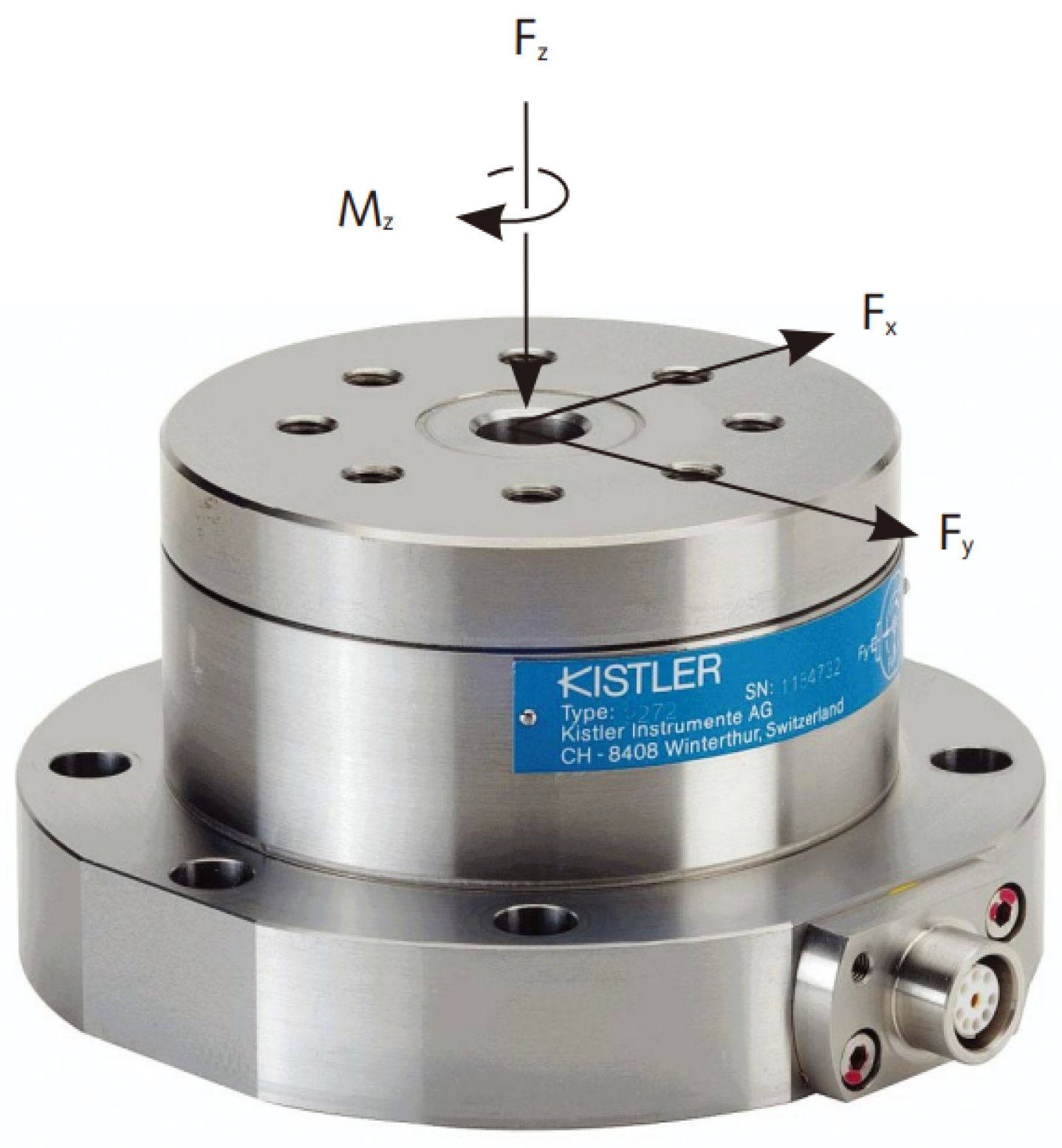
Toshiyuki et al. collected three-axis force signals through experiments, extracted multidimensional features using a variety of data preprocessing techniques, and used neural network algorithms to comprehensively analyze these features, successfully realizing tool wear monitoring [
6]. Patra, K., et al. studied the changes in cutting force with the increase in the number of holes processed under different feed rates and drilling speeds for force signals in micro-scale machining processes and established a prediction model using artificial neural networks. The experimental results show that the model based on cutting force data has a high consistency with the prediction of the actual number of holes drilled [
7].
Dimla et al. also collected three-axis force signals in the experiment; conducted a static analysis of the forces in the X, Y, and Z directions; and compared them with vibration signals and power signals. The study found that the cutting force signal is much more sensitive to tool wear than the vibration and power signals. In particular, among the three-axis force signals, the feed force direction signal is the most sensitive to tool wear [
8].
- (2)
Vibration signal
As tool wear increases, the cutting force in the cutting process also increases, resulting in increased vibration of the cutting system, and in severe cases, even making the cutting process unable to continue. Since vibration signals are sensitive to tool wear and easy to measure, it is very common to use vibration signals to identify tool wear status in industrial applications.
Ratava, J., et al. collected vibration signals in intermittent cutting experiments; constructed a tool wear classification model based on cutting depth, feed speed, and acceleration signals; associated the vibration signals with tool deflection and cutting force signals; and used this model to identify tool wear status [
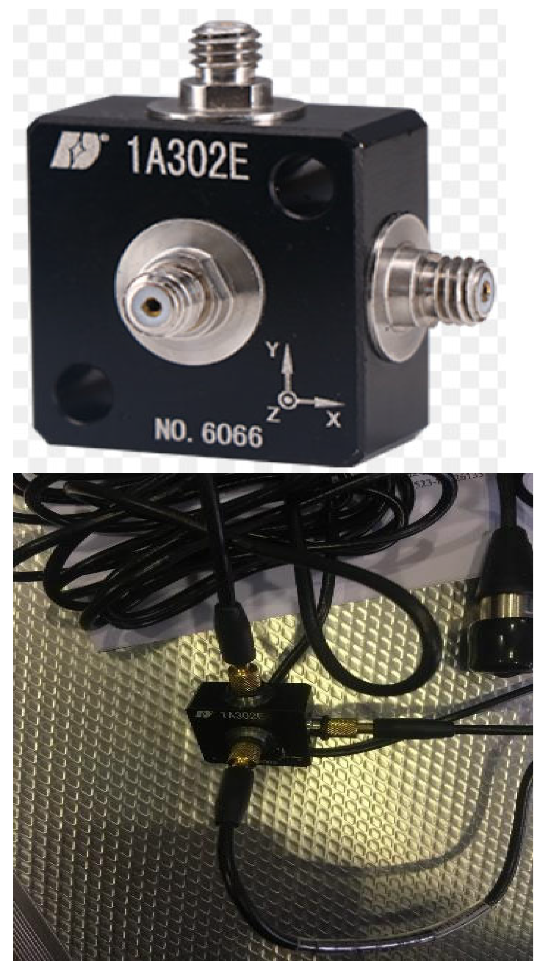
9]. Dai Wen et al. collected three-axis vibration signals during milling processing. During data processing, they used a stacked sparse autoencoder network to optimize and reduce the time domain and frequency domain features and used an adaptive step-size cuckoo algorithm to optimize the LS-SVM model parameters. They established a tool wear status prediction model based on vibration signals and achieved a high prediction accuracy [
10].
- (3)
Current and power signals
Tool wear increases the friction between the workpiece and the tool, which will not only increase the motor current but also increases the load power, which will eventually manifest as an increase in the total spindle power. Using current and power signals to monitor tool wear is a convenient method. Through the OPC UA server and Ethernet connection, the power data of the machine tool during the cutting process can be obtained in real time, while avoiding the influence of factors such as cutting, machine tool vibration, and tool temperature change. However, in finishing and semi-finishing cutting, the changes in machine tool power and current caused by tool wear are not obvious, and there is a certain hysteresis. Therefore, this method is more suitable for processing occasions with large cutting consumption [
11].
Li Congbo and colleagues analyzed the relationship between cutting power and tool wear and verified the influence of processing parameters on cutting power through experiments. On this basis, a regression model between cutting power, processing parameters and tool wear was established, and an online tool wear monitoring system with the real-time alarm threshold updates was developed using this model [
12]. Romero-Troncoso and colleagues constructed a theoretical model between power, current, and tool wear and conducted cutting processing experiments. The experimental results show that during the wear process of the tool from the new state to the passivated state, the machine tool power increases by about 20%, indicating that the tool state can be monitored by observing the change in machine tool power [
13]. Yang Tao and colleagues established a mathematical model for extracting cutting power from machine tool power and, combined with workpiece quality information, proposed a tool change strategy suitable for mass production. On this basis, tool change decision software was also developed [
14].
Lin Yang analyzed the milling force signal generated during high-speed milling by applying wavelet transform, successfully extracted the energy distribution characteristics of different frequency bands, and constructed a preliminary feature model based on this [
15]. Subsequently, he used an unsupervised learning network to teach these feature models, and finally used deep learning technology to predict the wear state of the tool. On the other hand, He Donglei and others collected acoustic emission signals in milling processing experiments and proposed an improved EEMD method to process these signals and extract the first six IMF components from them [
16]. They further extracted the corresponding Shannon entropy features based on different stages of tool wear and established a feature model. Finally, they used support vector machine technology to identify different stages of tool wear.
Cao Dali and others proposed a tool wear state recognition model based on convolutional neural networks to solve the problem of feature extraction in tool wear state recognition [
17]. The model used a deep learning network to perform adaptive feature extraction, effectively avoiding the data loss problem that may occur in the traditional manual feature extraction process and was able to mine subtle features that are not easy to detect in the signal. The research results show that the model has improved both recognition accuracy and generalization ability.
Xie Yangyang et al. used the frequency domain signal of the acoustic emission signal as an input to construct a double hidden layer stacked denoising autoencoder network and used a supervised training method to globally fine-tune the network, achieving the high-precision recognition of tool wear status [
18].
However, the existing tool wear monitoring methods still have some shortcomings. Although the direct monitoring method is accurate, it requires shutdown measurement, which significantly affects production efficiency. Although the indirect monitoring method can be used in real time during the processing process, the single sensor signal can only reflect local information and is easily interfered with by the outside world, resulting in low monitoring accuracy.
In view of the shortcomings of the existing methods, this paper proposes a tool wear state recognition model based on particle swarm optimization (PSO) and least squares support vector machine (LS-SVM), namely the PSO-LS-SVM model. The model extracts key feature information reflecting the tool wear state by integrating data collected by multiple sensors such as vibration signals and force data and optimizes the feature vector using dimensionality reduction techniques, such as principal component analysis (PCA), to reduce the complexity of the feature space. At the same time, the LS-SVM model parameters are optimized by particle swarm algorithm to further improve the recognition accuracy and adaptability of the model.
4. Experimental Analysis
4.1. Feature Extraction and Optimization
4.1.1. Time Domain Characteristics
The time domain analysis of signals refers to the analysis of the signals in the time domain and ultimately expressing the changing state of the signals as a parameter. It is the most basic and easy-to-understand form of expression. Moreover, no matter whether the frequency band of the signal is high or low, it can be extracted using the time domain analysis method [
34]. The elements in the time domain can be divided into two types according to their dimensionlessness. On this basis, the characteristic signals in the time domain are selected.
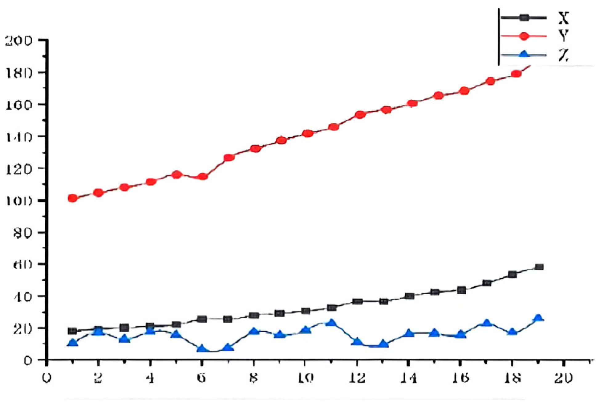
In order to observe the general changes in the signal time domain characteristics, the time domain characteristics of each pass were calculated according to the formula in
Table 3, and the relationship between certain time domain characteristics and the number of passes (i.e., cutting time) was obtained as shown in
Figure 8.
By analyzing the results of feature extraction, the results show that the dimensionless method can better characterize the wear status of the tool; in particular, the Y-axis, which is the feed direction, is closely related to the tool wear, and the X-axis, which is the vertical direction, is closely related to the tool wear. The feed signal is related to the loss of the tool. However, the Z direction signal in the time domain cannot reflect it directly. Only when the tool is worn will the stability of the system decrease. Compared with the dimensionless characteristic signal, the sizing characteristics do not change significantly with the increase in tool wear.
4.1.2. Frequency Domain Characteristics
The vibration and force signals in milling processing are affected by factors such as spindle rotation, cutting, and tool wear. Therefore, during the machining process, the signal changes in a cycle. The tool wear information that can be obtained by the traditional time domain analysis method is very limited, and the time domain analysis method can only reflect the vibration and force amplitude changes that occur with the tool wear state. The actual signal often contains information in multiple frequency bands. Therefore, the frequency domain analysis method must be used to conduct a more in-depth study. In the frequency domain, feature extraction is to first perform FFT transformation on the signal and then calculate its characteristic quantity in the frequency domain based on the expression of the eigenvalue. The usual frequency domain characteristics are as follows:
Center of gravity frequency:
This can reflect the changes in the center of the tool vibration signal spectrum under various working conditions.
This can explain the discreteness of the signal.
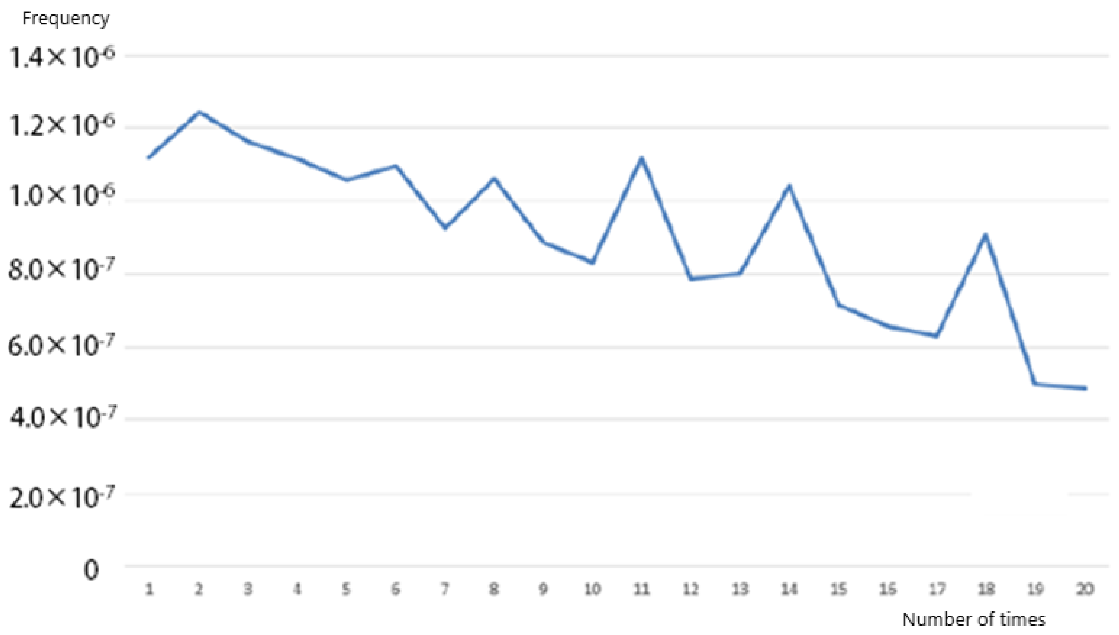
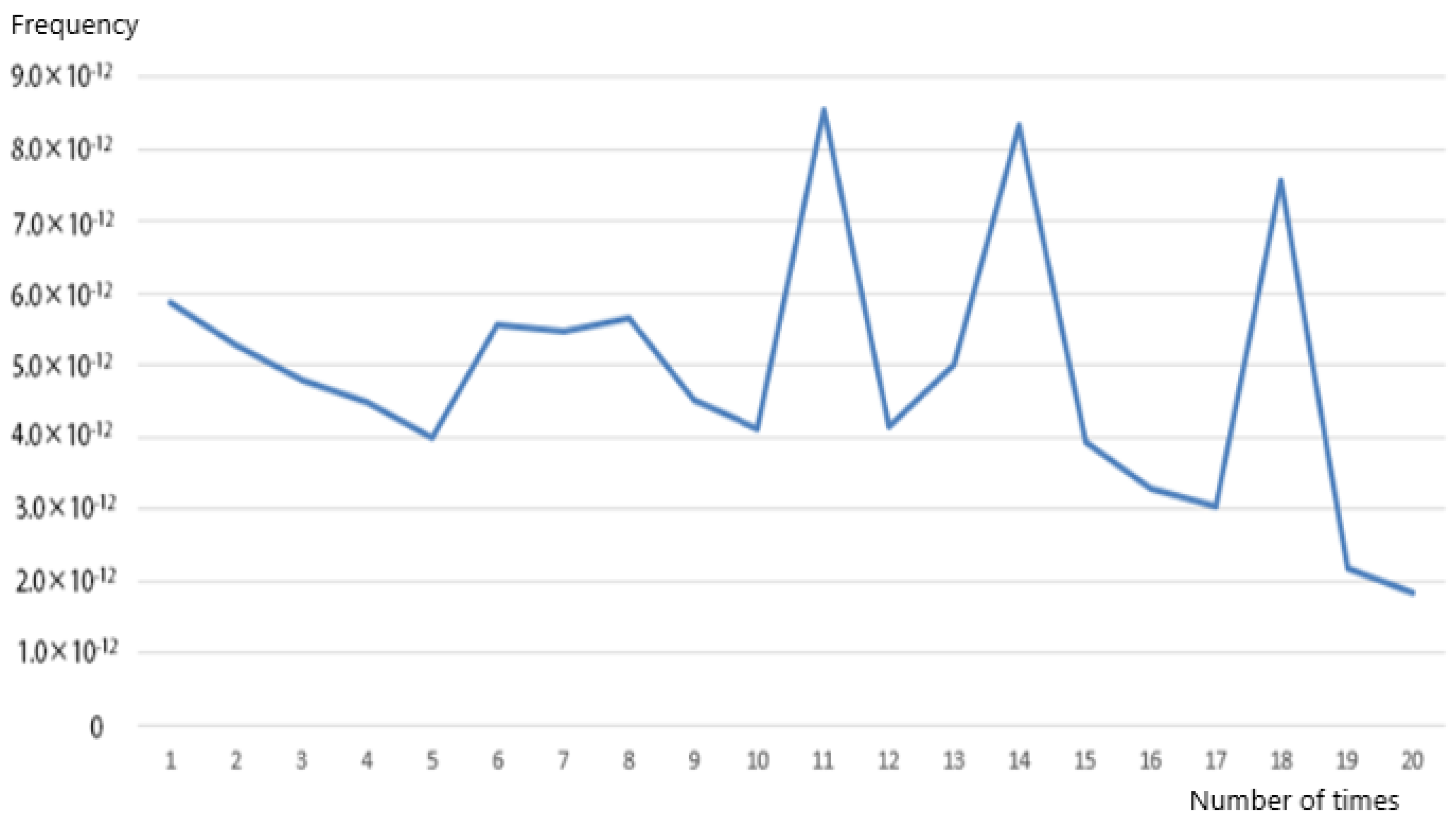
During the cutting process, according to the average frequency during the cutting process, this can be used to characterize the vibration frequency of the tool during the cutting process. Taking the vibration signal in the feed direction as an example, it can be seen from
Figure 9 and
Figure 10 that when the number of tool movements increases, its center frequency also decreases; during the initial wear process, the average frequency and frequency of the system do not change, although there are significant changes in the middle and late stages of wear. This is mainly because the stability of the system will decrease during the wear process, and the frequency response characteristics are more sensitive to the stability of the system; thus, in the late stages of wear, the frequency characteristics of the system show large fluctuations. Existing research shows that during the cutting process, as the cutting speed increases, the changing pattern will gradually intensify. However, based on this changing trend alone, it is impossible to construct an accurate tool wear characteristic model.
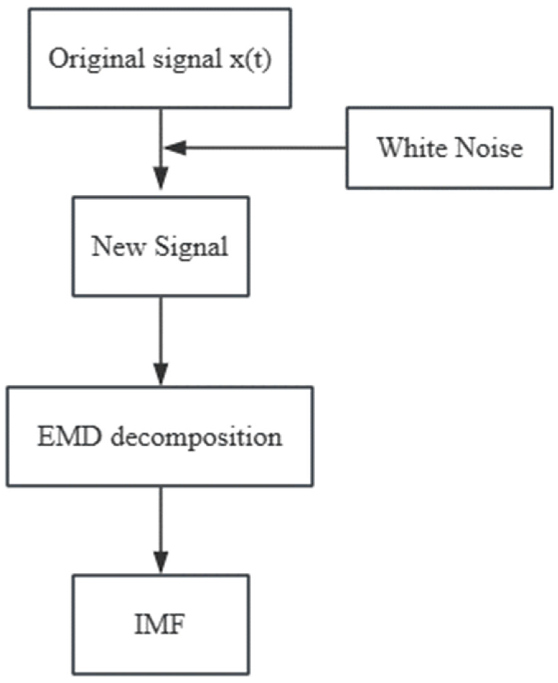
4.1.3. Time–Frequency Domain Feature Extraction Based on EEMD
In view of the complex characteristics of the tool wear process, during analysis, changes in the time domain and frequency domain must both be taken into account. The existing wavelet analysis and empirical mode decomposition (EMD) are compared with wavelet decomposition (WT). The EMD algorithm does not need to set the basis function in advance and only decomposes according to the time scale characteristics of the signal itself. Therefore, it shows unique advantages when processing non-steady-state data such as vibration and force perception. However, when using the empirical mode decomposition method to decompose the signal, modal aliasing will occur. To address this problem, researchers have proposed a mode confusion problem based on ensemble empirical mode decomposition (EEMD). The basic idea of this method is to introduce Gaussian white noise into the original signal so that the signal maintains good continuity at multiple scales and effectively suppresses the mode mixing phenomenon. To address this problem, this paper uses EEMD to decompose the vibration and force signals and extract features in the time domain and frequency domain. The specific EEMD algorithm steps are shown in
Figure 11.
Here, the detailed steps of EMD are as follows:
- (1)
First find all local extreme values of the original signal X(t);
- (2)
Use the cubic spline curve to fit the local maximum and minimum points to obtain the upper and lower envelopes and use u(t) to represent the upper and lower envelopes. Then, based on the upper and lower envelopes, obtain the average curve m(t):
- (3)
Let h1 represent the difference between the mean values of the initial data X(t) and m(t), then
At this time, h1 is regarded as a new initial signal, and the above three steps are repeatedly performed until h1 is satisfied.
Across the entire time range, the number of function zeros and local poles is the same or differs by one at most; in the signal segment, the average of the upper and lower envelope surfaces is 0. At this point, h1 is the first-order IMF at the screening location, as denoted by C1. In general, C1 contains the highest frequency component of the original signal.
- (4)
Remove a maximum frequency component from the original signal to obtain a difference signal, r1:
Taking
r1 as the new initial signal, repeat the above three steps until the residual signal obtained is a monotonic function without a maximum value and the IMF component can no longer be screened.
- (5)
Finally, mathematically speaking, the original signal X(t) can be expressed as the sum of n IMFs and 1 residual.
Of these, rn(t) is used as a parameter to express the average trend of the signal, and Cj(t) represents the IMF components, ranging from high frequency to low frequency.
4.1.4. Feature Optimization Based on PCA
On the basis of the above research, the characteristics of load, vibration, and other signals were analyzed, respectively, and finally, 90 time domain features were obtained, which are labeled sT. There are 18 feature vectors in the frequency domain, and these are represented by hT. In total, 108 time–frequency feature vectors are proposed, which are labeled Tsh. These three feature vectors are connected in sequence to form a new joint multi-feature vector denoted as Tcs, so that the multi-feature vector is 216. If Tcs is used as a characterization vector of tool wear state, it not only requires a large amount of data but also contains a large number of redundant feature vectors, which will inevitably reduce the recognition efficiency and recognition accuracy. In view of the redundant and irrelevant characteristics existing in the joint multi-feature vector, the PCA method is used to optimize it.
The core idea of this method is to construct a series of new variables based on the original attributes by linearly combining the original attributes, making their number much smaller than the original data, and to keep the effective information in the original data as much as possible, remove redundant information, and achieve dimensionality reduction in the projection space. By constructing the orthogonal relationship between the new variables, the correlation between the original variables can be effectively removed and the dimension of the data can be greatly reduced. The new features of dimensionality reduction obtained through principal component analysis are shown below.
The new feature cannot fully represent the original feature. It is a linear combination of several interrelated old features. The two elements are perpendicular to each other, not interrelated. The new feature size is much smaller than the original feature size. The feature dimension reduction optimization method using principal component analysis is as follows:
- (1)
Standardize the feature vector. Here, max–min normalization is used. The calculation formula is as follows. The standardized data are used to generate the sample matrix X.
- (2)
Calculate the mean of the sample matrix X:
- (3)
Calculate the covariance matrix for the sample matrix X:
- (4)
A new mathematical representation model is established.
PCA is used to reduce the dimension of the original feature vector and obtain its principal component coefficient matrix
C:
The contribution of the system is sorted according to the new vector reconstructed after dimensionality reduction. The number of principal components is determined by principal component variance–cumulative contribution (CPV), and its value can be determined by the formula below. The number of principal components is selected according to the criterion that CPV is no less than 95% to ensure the completeness of the information.
The first 10 principal elements were selected as new eigenvectors and were described to obtain new eigenvectors.
4.2. Analysis of Test Results
Before inputting the data into the model, they must be split into a training set and a test set. Taking the milling cutter as an example, according to the vibration data from its entire lifecycle, 70% of the samples are used as training samples and 30% of the samples are used as test samples at a ratio of 7:3. The specific division method is as follows: expand the data through the sliding window one by one, rearrange the data after the sliding window, and then partition them; then choose the random sampling partition method.
- (1)
Impact of input on recognition effect
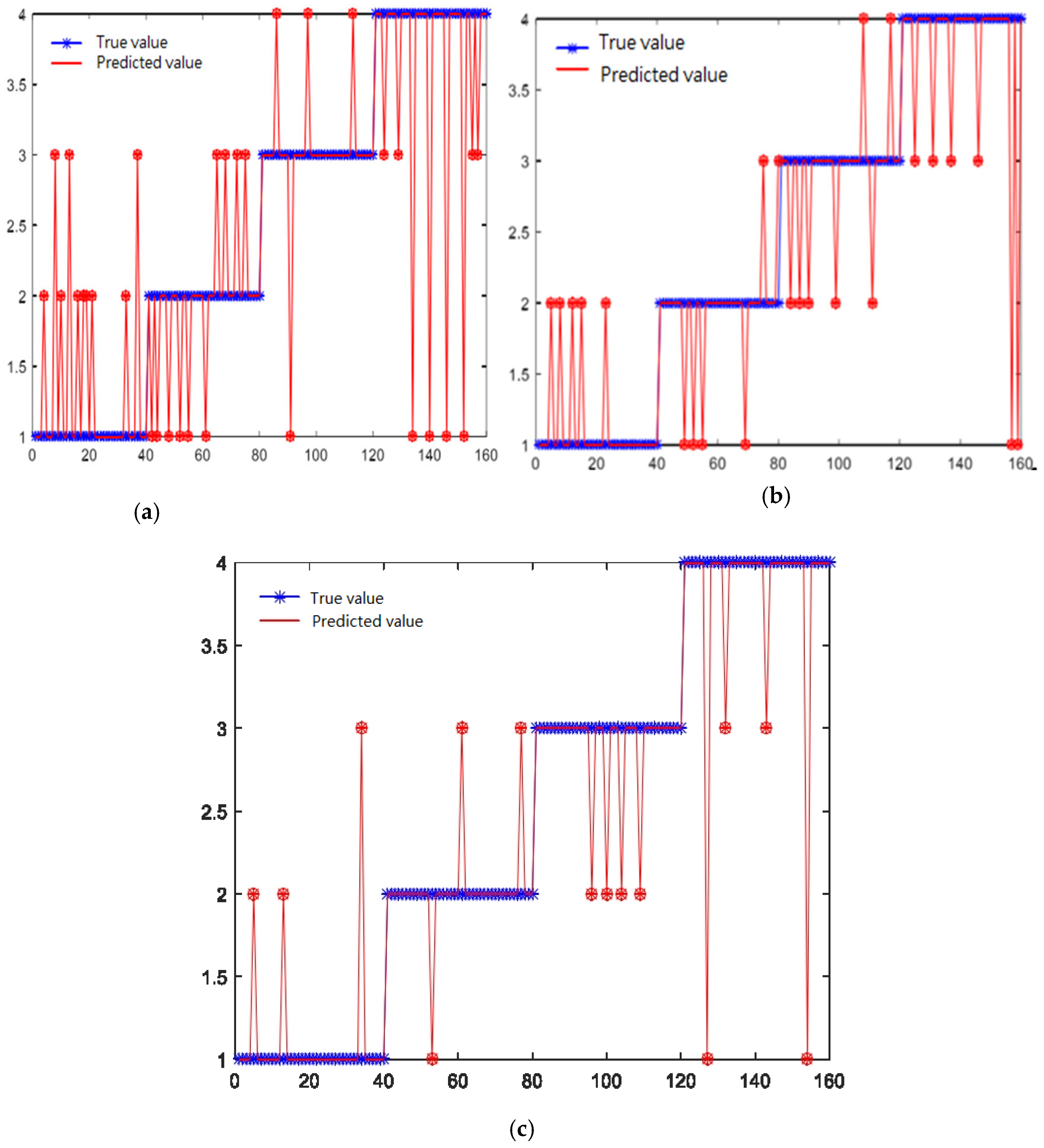
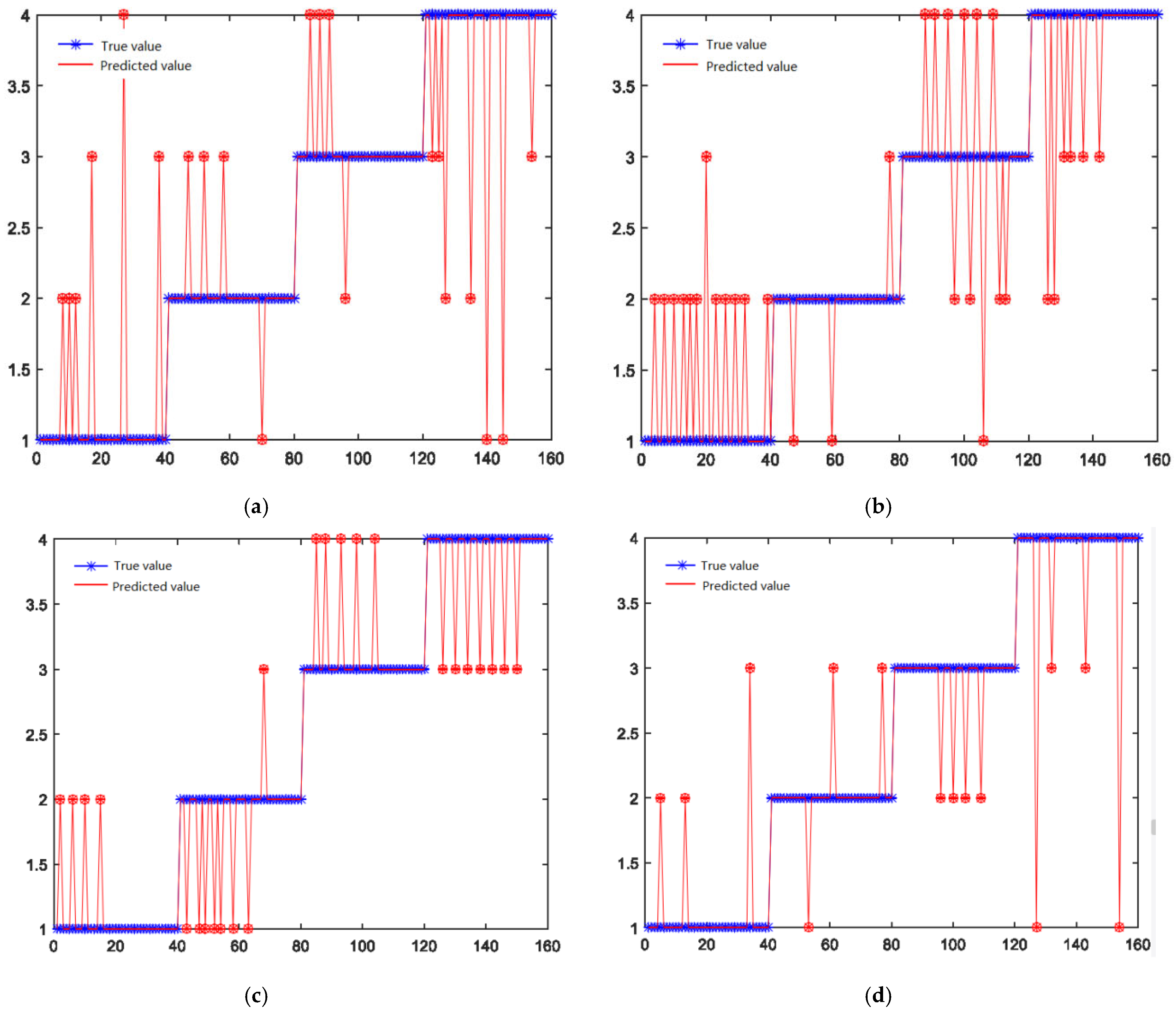
To solve the above problems, this paper adopts the PSO-LSSVM method, takes the characteristic information of single and multiple signals as input, and uses the PSO-LSSVM method to experimentally study the multiple signal recognition method. The initial wear states (1, 2, 3, 4) are marked as states 1, 2, 3, 4. The recognition results are shown in
Figure 12.
The recognition accuracy of each stage for different input signals is shown in
Table 4.
The results show that when a single signal is used as input, its recognition rate is lower than that of multiple signal inputs. From the recognition situation of each stage, in the first two states, the recognition rate of the force signal is relatively high, and the recognition rate in the last two states is mainly determined by the force signal. This is because in the early stage of wear and steady state, the tool is relatively sharp, making the whole process more stable. Only the vibration signal is used for identification, and its feature resolution ability is not strong. The force signal can intuitively reflect the friction coefficient during the tool wear process. In the first two stages, it shows better recognition results than the vibration signal. However, when the wear is advanced, the contact area between the tool tip and the workpiece becomes larger, thereby reducing the stability of the system. At this time, the sensitivity of the vibration signal to force is greater than that of the force signal, and the complexity of the vibration signal is also high. This characteristic is reflected in the entropy value in the time–frequency domain. Using vibration and force signals as monitoring signals can overcome the incomplete information that can be reflected by a single signal, thereby improving the accuracy of model identification. However, when two different signals are input, it will lead to an increase in feature dimensions and a decrease in performance, so it needs to be optimized.
- (2)
Impact of input characteristics on recognition results
The PSO-LSSVM method is used to learn and identify the time domain, frequency domain, time domain, frequency domain, and multiple features at once. The final identification results are shown in
Figure 13, and the identification rate of each specific stage is shown in
Table 5.
The results show that using multiple features as the input of the model can improve the overall recognition rate and the recognition rate at each stage. Existing research mainly focuses on the modeling of a single type of feature, which contains less tool wear information and cannot fully reflect the change law of various physical parameters under the tool wear state. Although the training and recognition efficiency will decrease when multiple features are introduced into the modeling, it contains a large amount of tool wear information and can effectively improve the recognition accuracy of the model.
- (3)
The impact of optimal feature selection on recognition results
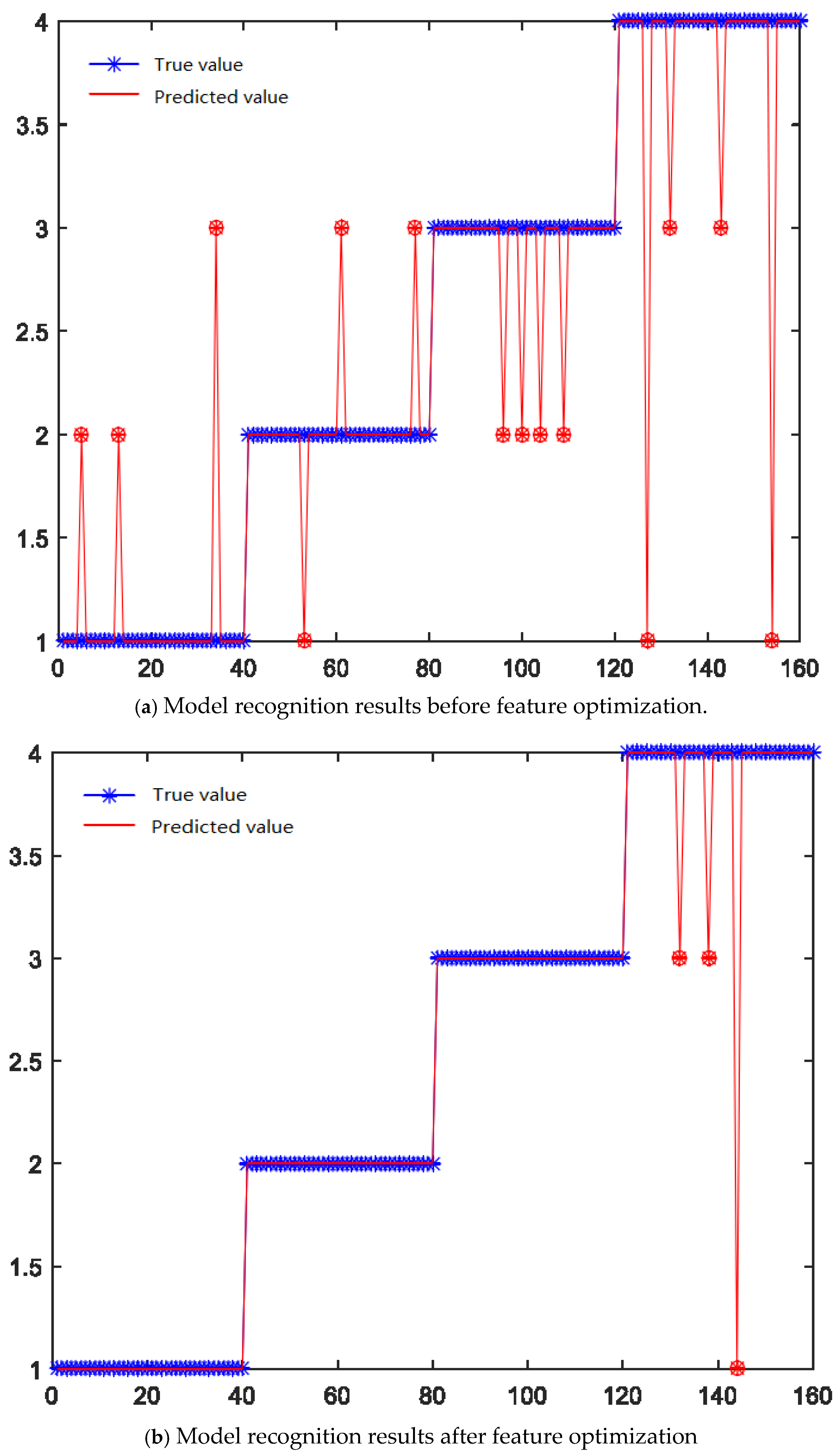
Although the simultaneous input of multiple sources and multiple features can effectively improve the model recognition accuracy, the simultaneous input of multiple sources and multiple features will inevitably lead to an increase in feature vectors and redundant and irrelevant information, which is not conducive to the identification of tool wear status. To this end, this paper further optimizes the features, takes the feature vectors before and after optimization as input, and uses PSO-LS-SVM as input to realize the identification of tool wear status. Its recognition results are shown in
Figure 14, and the recognition rate of each specific stage is shown in
Table 6.
The results show that before feature optimization, the overall recognition rate can reach 91.6%, and after feature optimization, the overall recognition rate can reach 98.1%. The overall recognition rate and the recognition rates at each stage have improved to varying degrees. In addition, through feature optimization, a large number of redundant and irrelevant features are removed, and the original 216 dimensions are reduced to 10 dimensions, thereby greatly improving the training and recognition efficiency of the model.
- (4)
Impact of parameter optimization on identification effect
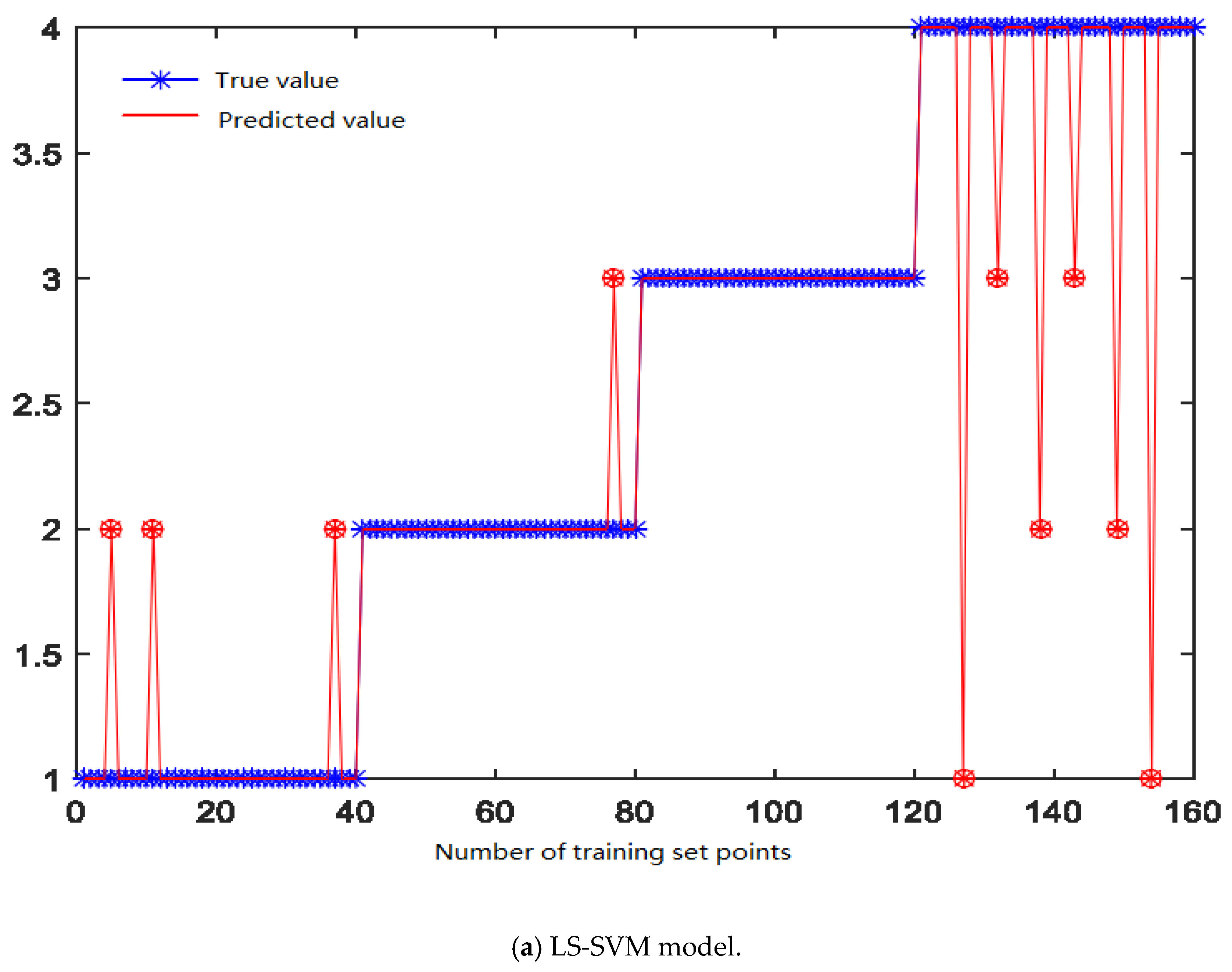
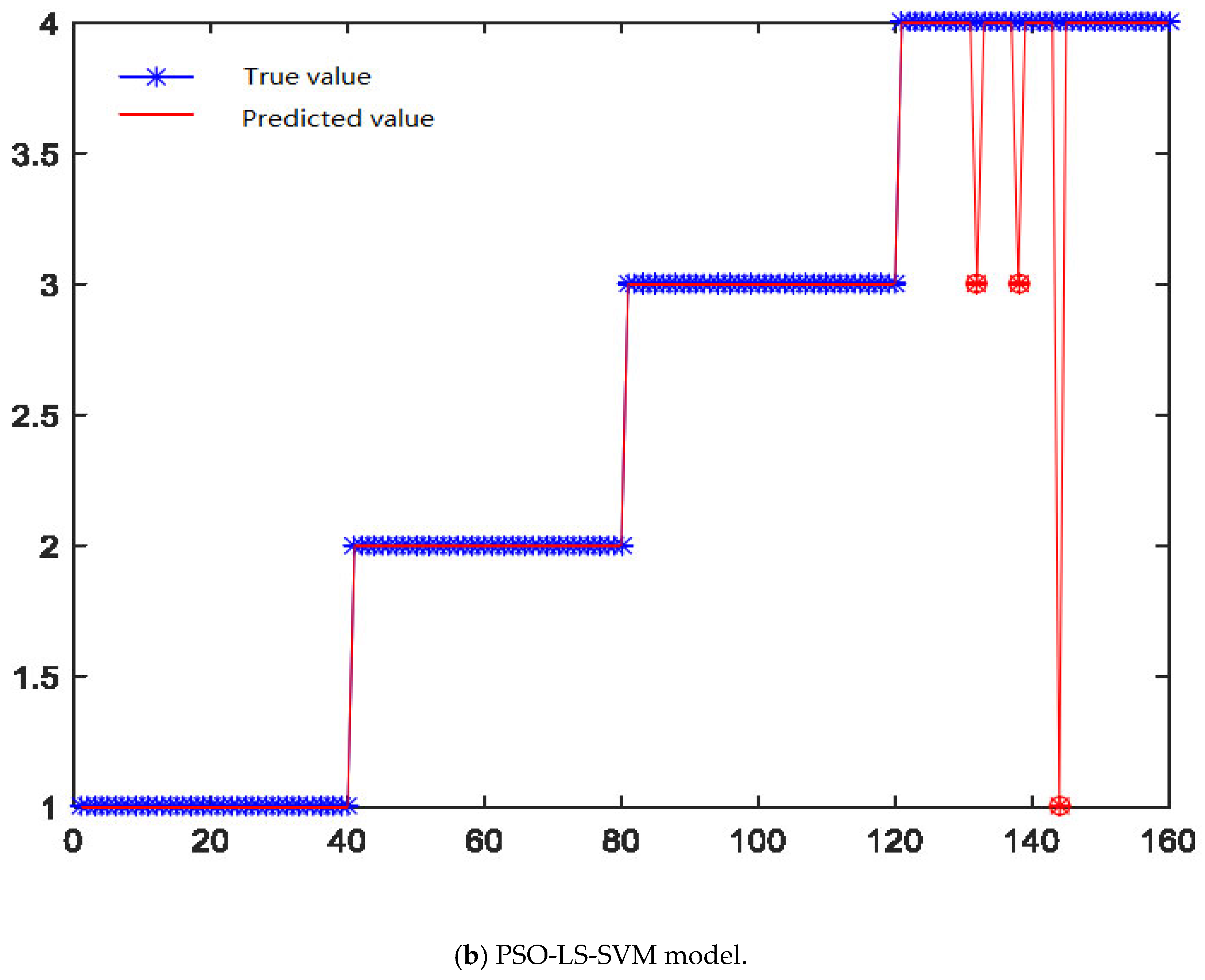
The optimal feature vector is used as the input of the LS-SVM and PSO-LS-SVM support vector machines, which are then studied and identified. The final recognition effect is shown in
Figure 15.
The experimental results show that the recognition rate of LS-SVM optimized by this method is significantly higher than that of unoptimized LS-SVM. Compared with the unoptimized LS-SVM, the overall recognition rate of PSO-LS-SVM reaches 98.6%, while that of the unoptimized LS-SVM is only 92.4%. The results show that after the optimization of the particle swarm algorithm, the recognition accuracy of the entire model and the recognition accuracy of tool wear at each stage are improved. The LS-SVM optimization method based on PSO can better solve the problems existing in LS-SVM in practical applications. As shown in
Table 7.
5. Conclusions
In this study, a wear prediction model based on particle swarm optimization (PSO) and least squares support vector machine (LS-SVM), namely the PSO-LS-SVM model, was successfully developed and verified. The model fuses data from multiple sensors, including vibration signals and force data, and extracts key feature information reflecting the tool wear state. By using principal component analysis (PCA) for dimensionality reduction and feature optimization, the model significantly improves the distinguishability of features and reduces the complexity of the feature space.
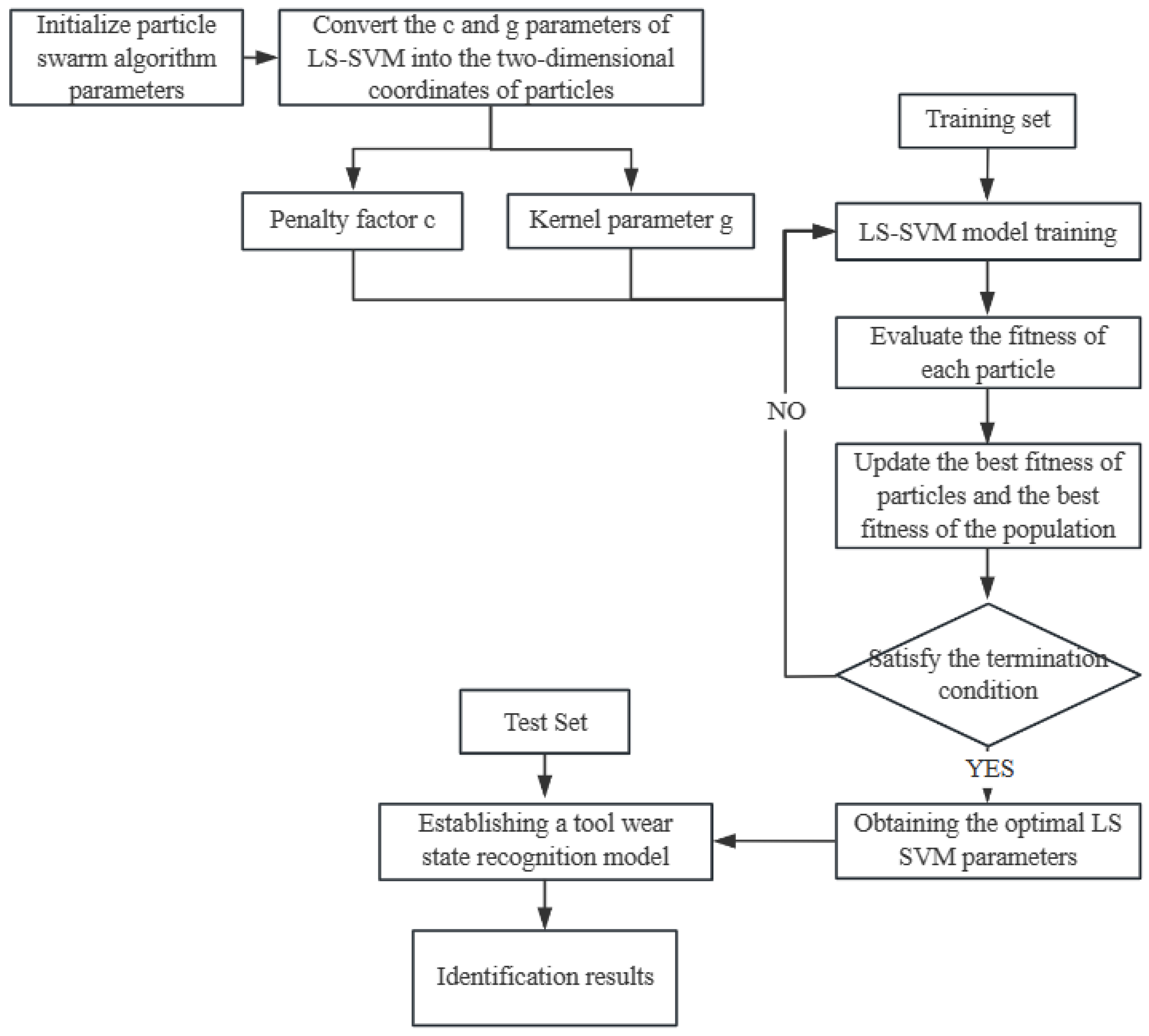
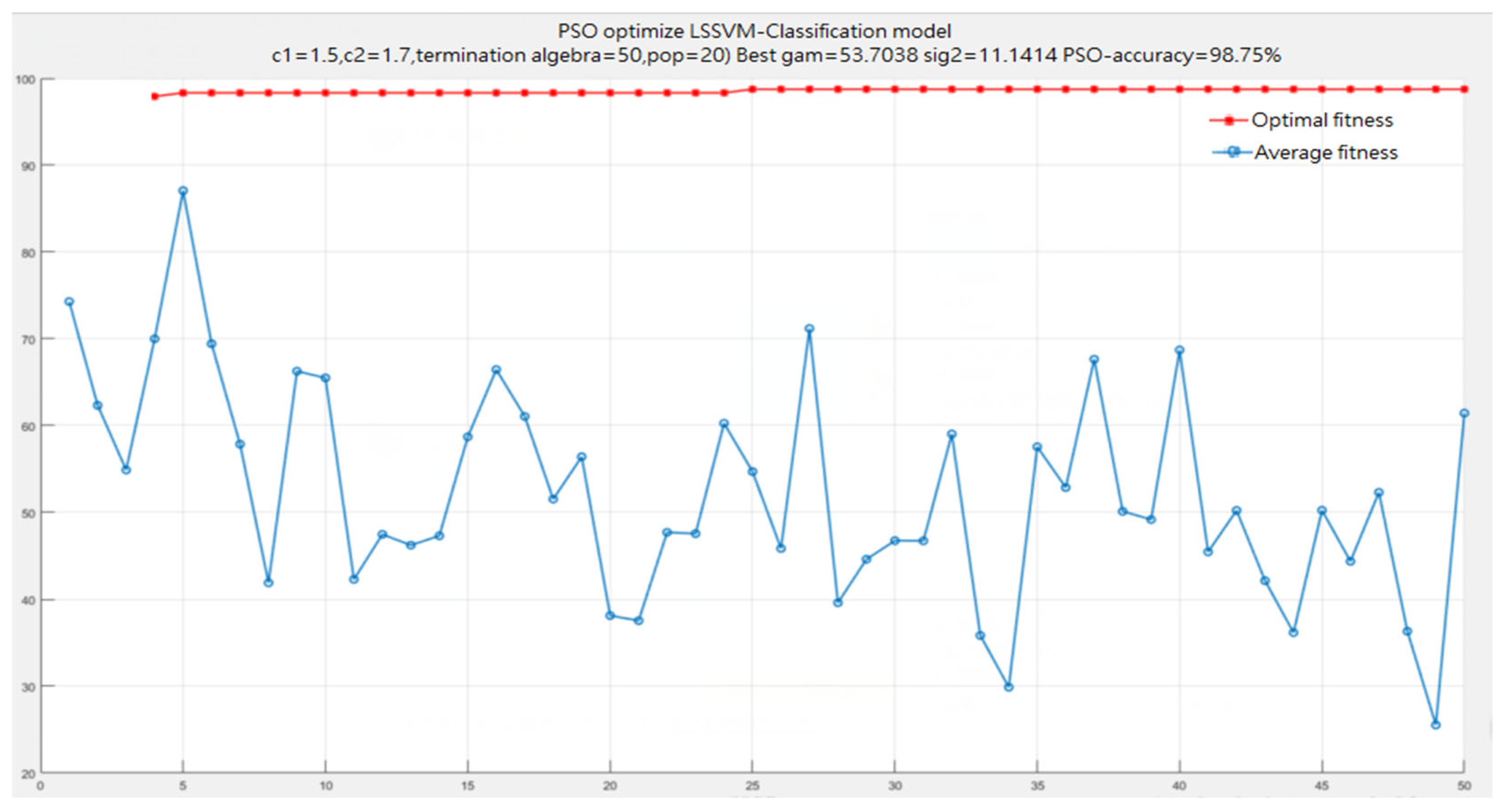
The PSO-LS-SVM model optimizes the model parameters to adapt to the given training sample set through the two-dimensional coordinates (c and g) of the particle swarm algorithm, and its effectiveness is demonstrated. The optimal fitness of the particles is continuously updated by iteratively calculating the fitness and comparing it with the historical optimal fitness, so as to determine the global optimal solution and accurately identify the tool wear state. Experimental results demonstrate that the PSO-LS-SVM model shows high accuracy and good performance for tool wear state identification.
In summary, the PSO-LS-SVM model provides a promising method for tool wear prediction, which has significantly improved efficiency and accuracy over traditional methods. This study contributes to the field of CNC machining and provides a reliable and effective tool wear prediction model that can be integrated into smart manufacturing systems to optimize production processes and maintain high quality standards.


