Abstract
Brain–computer interfaces (BCIs) provide a direct communication pathway between the central nervous system and external environments, enabling human–machine interaction control. Among them, event-related potential (ERP)-based BCIs are among the most accurate and reliable BCI systems. However, current mainstream classification algorithms struggle to eliminate calibration requirements and rely heavily on costly labeled data, limiting the practical usability of ERP-based BCIs. To address this, the development of unsupervised algorithms is critical for advancing real-world BCI applications. In this study, we propose the spatio-temporal equalization sliding-window distribution distance maximization (STE-sDDM) algorithm, which introduces spatio-temporal equalization (STE) to unsupervised ERP classification for the first time and integrates it with a novel unsupervised classification method, sliding-window distribution distance maximization (sDDM). STE estimates and removes colored noise interference in background noise to enhance the signal-to-noise ratio of inputs for sDDM. Meanwhile, sDDM leverages an enhanced inter-class divergence metric based on the ergodic hypothesis theory, utilizing sliding windows to emphasize temporally discriminative features, thereby improving unsupervised classification accuracy. The experimental results demonstrate that the integration of STE and sDDM significantly enhances ERP feature separability, outperforming state-of-the-art unsupervised online classification algorithms in spelling accuracy and the information transfer rate (ITR), facilitating more accurate and faster plug-and-play real-time control for BCI systems. Additionally, static spatio-temporal equalizer architectures were found to outperform dynamic architectures when combined with this framework.
1. Introduction
Brain–computer interfaces (BCIs) enable direct communication between the human brain and external devices by identifying brain signals and translating them into control commands, leading to revolutionary advancements in fields such as rehabilitation, smart prosthetics control, and human–computer interaction [1,2,3]. For instance, in the rehabilitation domain, BCIs can capture patients’ motor intentions in real time, triggering mechanical hand movements as feedback to form a “brain–machine–body” closed-loop training system [4,5,6]. This helps stroke or spinal cord injury patients rebuild damaged neural pathways, significantly enhance neural plasticity, and accelerate motor function recovery. Event-related potentials (ERPs), which are evoked electrophysiological responses time-locked to external stimuli, are widely utilized in BCIs, with the P300 component emerging approximately 300 ms post-stimulus [7,8,9,10]. ERP-based BCIs (ERP-BCIs) employ machine learning (ML) techniques to extract features and classify ERPs, enabling command decoding and system control [11,12].
ML approaches for ERP-BCIs include supervised, semi-supervised, and unsupervised learning. Supervised methods (e.g., linear discriminant analysis (LDA), support vector machines (SVMs), and neural networks like EEGNet and DeepConvNet) require labeled training data [13,14,15,16,17,18]. Despite their accuracy, dependence on calibration phases increases user burden and time costs [19]. While transfer learning and semi-supervised methods reduce calibration needs, they remain constrained by labeled data requirements and feature standardization challenges [20,21,22,23,24,25].
Unsupervised methods such as expectation maximization (EM), label proportion learning (LLP), and unsupervised mean-difference maximization (UMM) aim to overcome these limitations. Unsupervised ERP classification methods do not require ground-truth labels for initialization; instead, they autonomously construct classification models by leveraging the intrinsic variance within the input data. This characteristic makes them well suited for calibration-free online classification scenarios. The EM algorithm is based on the principle of expectation maximization, where a Gaussian classifier is randomly initialized and iteratively optimized using Bayesian least-squares regression to estimate target probabilities and refine classifier parameters [26,27]. LLP modifies the paradigm by adjusting the probability of the target across different events, constructing a linear equation for the mean of the target and non-target events. This ensures convergence to the true average value after accumulating a sufficient number of epochs, although it is constrained by specific paradigms [28,29]. Unlike classical binary classification approaches, UMM aggregates classification results over an entire spelling trial rather than making single-event decisions. It assumes each possible symbol as the target in a given trial and selects the optimal hypothesis that maximizes the Mahalanobis distance between ERP target and non-target averages. While UMM has demonstrated superior classification performance in visual ERP datasets, its performance deteriorates in auditory and clinical environments [30]. Despite progress, these methods face challenges such as spatio-temporal feature weighting and colored noise interference.
Therefore, this study proposes the spatio-temporal equalization sliding-window distribution distance maximization (STE-sDDM) algorithm. First, an improved approach, the Sliding-Window Distribution Distance Maximization (sDDM) method, is introduced within the UMM framework. This method enhances the measurement of inter-class differences by incorporating two key aspects: the dispersion of intra-class distributions and the similarity among multiple events within the target class. By more accurately assessing the differences between the target and non-target hypotheses, this approach improves classification performance. Additionally, the introduction of a sliding window facilitates the extraction of time-varying features, allowing for the identification of temporal segments with significant inter-class differences and ensuring greater emphasis on these critical periods. Second, leveraging the respective advantages of the spatio-temporal equalizer and ERP-based unsupervised classification algorithms, the sDDM method is integrated with the spatio-temporal equalizer to construct a simple yet effective online classification framework. The STE technique employs a Multivariate Autoregressive (MVAR) model to characterize EEG background noise. The estimated parameters are then applied to the design of the spatio-temporal equalizer, which mitigates both spatial and temporal correlations in multi-channel EEG background noise. This process effectively eliminates colored components within the noise. To the best of our knowledge, this is the first application of spatio-temporal noise equalization techniques in ERP classification tasks based on unsupervised algorithms.
2. Methods
2.1. EEG Signal Model and Background Noise Estimation
EEG signals contain not only task-related neural activity but also substantial background noise, including spontaneous EEG activity and artifacts such as electrooculographic (EOG) and electromyographic (EMG) components. This background noise has been demonstrated to be colored and exhibits high temporal correlation [31,32]. Traditional signal processing methods often assume that background noise is uncorrelated Gaussian white noise. This assumption primarily stems from the fact that spontaneous EEG originates from the synchronized activity of large-scale distributed neuronal networks connected via synapses [33]. Due to its complex and diverse origins, it is often approximated as a Gaussian-distributed random signal based on the central limit theorem [34], facilitating EEG analysis. However, in reality, due to the volume conduction effect of the skull, electrical signals generated by brain activity undergo inevitable spatio-temporal aliasing during their propagation from the cortex to the scalp. Consequently, EEG signals recorded by extracranial electrodes typically exhibit significant spatio-temporal correlations.
The spatio-temporal correlation of EEG background noise is characterized by the following aspects: (1) nonzero spatial correlation among background noise recorded by different channels, (2) nonzero temporal correlation within a single channel, and (3) the stability of this spatio-temporal correlation over a certain period. Given these properties of background noise, STE is introduced to enhance the signal-to-noise ratio in unsupervised classification tasks [35,36,37]. Before each trial in the online experiment, the raw EEG signals are processed using an STE filter to suppress the spatial and temporal correlations of background noise across multiple channels. The equalized signals are then input into the sDDM algorithm for unsupervised classification.
To estimate the spatio-temporal correlation structure of background noise, it is necessary to extract EEG segments devoid of event-related components. An MVAR model is employed to characterize background noise, and the estimated parameters are subsequently used to design the spatio-temporal equalizer.
For this study, the following assumptions are made regarding EEG background noise:
- Task-related components and background noise components are independent of each other;
- Background noise exhibits short-term stationarity;
- Background noise can be approximated as zero-mean Gaussian noise with spatio-temporal correlations.
Based on the aforementioned considerations, the EEG signal containing task-related components can be modeled as follows:
where represents the raw EEG signal at time t, denotes the ERP component at time t, and represents the residual background noise at time t. The total number of time points in the EEG signal is denoted as . Assuming that the signal has a spatial dimension of L, we define .
To model these spatio-temporally correlated signals, an MVAR model is employed. EEG signals are significantly affected by volume conduction, leading to substantial spatio-temporal mixing. Compared to traditional techniques such as Principal Component Analysis (PCA) and Independent Component Analysis (ICA), which primarily rely on variance decomposition or assumptions of statistical independence, MVAR offers a key advantage in capturing temporal causality. This capability allows it to more accurately model the spatio-temporal dependencies of EEG signals, making it particularly suitable for background noise estimation when a sufficiently large data window is available. The background noise is represented using a P-order MVAR model as follows:
where represents the p-th coefficient matrix in the MVAR model, and denotes temporally uncorrelated noise at time t. Specifically, all L channels of are assumed to be independent and identically distributed (i.i.d.) Gaussian noise. Let be the spatial covariance matrix of , such that
Typically, the order of the MVAR model is determined using Akaike’s Final Prediction Error (FPE) criterion [38] or Schwarz’s Bayesian Criterion (SBC) [39]:
Within a predefined range of model orders, the optimal order P is selected as the one that minimizes either FPE(P) or SBC(P). In this study, the order of the MVAR model was set within the range of [4,16], with the optimal order determined using the FPE criterion.
2.2. Design of the Spatio-Temporal Equalizer
To eliminate spatio-temporal correlations, a filter bank comprising P + 1 FIR filters can be designed to equalize the EEG signals. This set of filters is referred to as the spatio-temporal equalizer.
However, to design the spatio-temporal equalizer, it is necessary to obtain the known background noise component . In the context of unsupervised online classification, it is not possible to precisely estimate the signal component from labeled data and then derive an estimate of by subtracting from the raw signal . As an alternative, we can select a segment of pure background noise that is sufficiently close in time to and free of task-related components. This segment, denoted as , corresponds to time point and spans time points, i.e., . Based on the assumptions about background noise, including the independence of task-related components and background noise, as well as the short-term stationarity of the latter, it can be assumed that exhibits the same spatio-temporal correlation as and thus can be used as a substitute for in the estimation of the MVAR model.
The optimal P-order of the MVAR model is determined for the background noise segment , and the P-order MVAR model is estimated as follows:
From this, we can obtain the P parameter matrices and the residual noise , whose spatial covariance is denoted as . The spatio-temporal equalizer is defined as follows:
where represents the whitening matrix derived from the spatial covariance matrix, and is the L-dimensional identity matrix. The spatio-temporal equalizer B ensures that the output of the noise after equalization satisfies the spatio-temporal decorrelation constraint. Consequently, B also ensures that , which shares the same spatio-temporal correlation as , will be decorrelated after equalization.
2.3. Application of the Spatio-Temporal Equalizer
The raw EEG signal is input into the spatio-temporal equalizer B, and the output of the equalizer is denoted as . The process of applying the spatio-temporal equalizer B to is represented as follows:
In this equation, represents the signal component after equalization, and denotes the residual noise after equalizing . Ideally, the output signal after equalization contains only the signal component and Gaussian noise , which is spatially and temporally uncorrelated. The spatio-temporal correlations of the noise are effectively removed.
It is important to note that, although we assume the independence between and , the correlation between the measured and in practical environments can only be minimized, but not eliminated. Therefore, in practice, the components of that are correlated with will be equalized, and the spatio-temporal correlation of will no longer perfectly match that of . In other words, the ERP features before and after STE will be altered.
2.4. Sliding-Window Distribution Distance Maximization
The sDDM algorithm is specifically designed for online EEG processing and unsupervised classification. It treats a single trial, which is the complete spelling process of one character in the spelling paradigm, as the minimal classification unit. The algorithm will be outlined from two perspectives: one from the viewpoint of a single trial and the other from the overall online decoding process.
2.4.1. Single-Trial Classification Process
To identify the true target, inspired by the UMM algorithm [30], we perform a one-by-one evaluation of all possible target hypotheses in the paradigm. This involves assuming target m as the correct one and evaluating the classification confidence for that hypothesis. We then iterate through all possible target hypotheses and select the one with the highest confidence as the classification result.
For a single trial, we define the input data as , where represents the number of channels, is the number of time points, and is the total number of samples in the trial. First, we center by removing the overall mean. The samples in can be categorized into two groups: (target) and (non-target). Alternatively, the samples can be divided into subsets , where , based on the type of associated flash code, corresponding to the possible flash types in the paradigm. Taking the row–column flash paradigm as an example, the above two partitioning methods result in a relationship: , where the assumed target in hypothesis m includes flash types and (with , and ).
In the previous UMM algorithm [30], the square Mahalanobis distance between the mean templates of and was used as a measure of hypothesis confidence. However, this metric overlooks two key aspects: (1) the within-class distribution information of and ; (2) the similarity between samples corresponding to different flashes within (i.e., and ). To better utilize these aspects, we propose an improved inter-class difference measure:
where represents the improved inter-class distance under target hypothesis m, which reflects the flash differences between and ; is the average intra-class distance under target hypothesis m. The calculations of and are as follows:
where is the total number of samples in class k, is the s-th sample of class k, is the mean template of class k, and is the Block–Toeplitz covariance matrix [15] derived from , of size . represents the operation of flattening a matrix into a one-dimensional vector, with the first dimension being of size 1.
In the above equation, , , and are the mean templates of , , and , respectively. The modified inter-class distance is influenced by the angle between the two vectors and . Compared to the simple inter-class mean distance used in UMM, this approach further reduces the interference caused by the simultaneous presence of target and non-target stimuli in and , leading to improved classification accuracy.
Additionally, the introduction of a sliding window allows for a better extraction of local features from the samples. Due to the temporal characteristics of ERPs, the difference between targets and non-targets does not appear to be equally significant across all time points. By incorporating a sliding window, we can obtain a distance measure for each window and emphasize the weights of the windows where the differences are most pronounced, thereby achieving a more reliable estimate of the inter-class differences.
With the sliding window applied, we divide the time window of the sample into overlapping windows and calculate an inter-class difference measure from each window, as given in Equation (10), where . Next, we need to obtain a single scalar value as the overall inter-class difference measure. However, since labeled data cannot be used effectively to estimate the window weight vector, we adopt the following method:
In this equation, the overall inter-class difference measure is computed as the -th power of the sum of the -th powers of the differences from all windows, essentially the -norm of the difference vector. We note that a simple average corresponds to an -norm with = 1. As increases, elements with larger absolute values exert a greater influence on the -norm result. This property allows -norm with > 1 to serve as an automatic weighting mechanism within the sliding window, without the need for explicit training.
Finally, the inter-class difference measure obtained from each target hypothesis m serves as the measure of classification confidence. We denote the hypothesis with the largest inter-class difference as hypothesis , the second largest as hypothesis , and so on, with the hypothesis with the smallest inter-class difference labeled as . Consequently, hypothesis , the one with the highest confidence, is selected as the most reliable hypothesis, and its corresponding label is output as the algorithm’s predicted label.
2.4.2. Fully Online Classification Process
Since the sDDM algorithm does not use labeled training data, leveraging information from previous trials is crucial for improving the online classification performance. We adopt an online updating strategy, utilizing pseudo-labels generated from past trials to enhance the classification capability of subsequent trials.
Consider the n-th trial (where n > 1) in the online process. To improve the classification performance of the n-th trial, the online update strategy will use the classification results from the previous n − 1 trials to adjust certain inter-class difference measures in the single-trial classification process, thereby incorporating the empirical knowledge accumulated from the earlier trials. In UMM, the update strategy focuses on adjusting and . However, in sDDM, this adjustment extends to , , , and .
Let any quantity that needs adjustment be denoted as . The adjustment can be written as follows:
In this equation, represents the adjustment before it is updated, and represents the adjusted value. The confidence for the n-th trial, , is calculated as follows:
After performing these calculations, we substitute in place of in Equations (10) to (12) where appears, continuing to compute the classification result. The adjusted value is then recorded for online updating in subsequent trials.
2.5. Spatio-Temporal Equalization Sliding-Window Distribution Distance Maximization (STE-sDDM) Algorithm Flow
The STE-sDDM algorithm leverages the spatio-temporal equalizer to enhance the signal-to-noise ratio of the input signals. As a result, its classification performance is expected to surpass that of the basic sDDM algorithm. As shown in works like [37], when introducing STE, a dynamic window is typically used to acquire the most recent noise segment corresponding to the current trial, effectively adapting to the changes in resting-state noise.
However, the sDDM algorithm relies on general ERP features learned from previous trials to strengthen its classification capability, primarily based on the assumption that ERP features remain stable throughout the online process. Given that the spatio-temporal equalizer’s adjustments also alter ERP features, we propose combining a stationary spatio-temporal equalizer with the sDDM algorithm to ensure that the ERP features remain consistent in every input. The framework of this approach is illustrated in Figure 1, which depicts the EEG data flow directed into STE and sDDM. The segment , spanning from the start of the data collection to the beginning of trial 1, is used as background noise to construct the static spatio-temporal equalizer B. Each trial’s input, , is then processed by B, producing , which undergoes further preprocessing before being fed into the sDDM classifier.
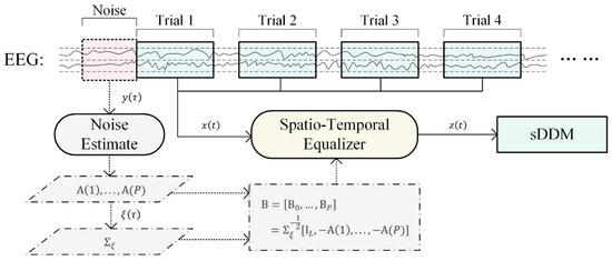
Figure 1.
Online decoding process of the STE-sDDM algorithm.
3. Experimental Design
3.1. Datasets and Data Processing
This experiment uses two datasets based on the VEP paradigm:
Dataset 1: This dataset was collected by our team for participation in the ERP task of the 2023 World Robotics Competition’s BCI Brain Control Competition (Document No.: ECUST-2022-054). It consists of EEG recordings from 42 participants, with each participant completing a random character spelling task across 32 trials. Each trial involves five rounds of randomly ordered flashes, with an inter-flash interval of 850 ms. Each sequence contains 12 flashes, and the flash encoding is defined based on binomial coefficients [40]. The flashes depict the appearance and disappearance of a face, each lasting for 75 ms (stimulus onset asynchrony, SOA = 150 ms). The paradigm interface displays a 6 × 6 character matrix containing the letters A–Z, numbers 1–9, and an underscore, totaling 36 spelling targets. EEG data were collected using the NSW364 wireless EEG system (Neuracle, NeuSen W series) with 59 channels at a sampling rate of 1000 Hz.
Dataset 2: This dataset comes from the ERP paradigm dataset of the OpenBMI repository, consisting of recordings from 54 healthy participants (aged 24–35; 25 females) [41]. EEG signals were recorded at a sampling rate of 1000 Hz using 62 Ag/AgCl electrodes, with the BrainAmp amplifier (Brain Products, Munich, Germany) and a nasal reference electrode, grounded to AFz. The electrode impedance was maintained below 10 kΩ throughout the experiment. The experimental paradigm follows the typical 6 × 6 row–column spelling design, spelling out 36 symbols (letters A-Z, numbers 1–9, and an underscore). The flash sequence uses a random set [42], with facial stimuli and ISI and SOA of 135 ms and 215 ms, respectively.
For both datasets, 32 channels are selected, and the data are initially segmented by trial to serve as the input for the signal processing steps. STE is applied to the continuous data of individual trials. We select the final segment of the data before the first trial as noise data, and both the noise and trial data are filtered to remove low-frequency components below 0.5 Hz to suppress baseline drift. The noise is then used to estimate the STE, and the trial data are input to STE for equalization.
Regardless of whether STE was applied, each trial’s data are filtered using a Butterworth filter in the 1–16 Hz range before unsupervised classification. For data segmentation, the time segment from 0 to 800 ms after each flash stimulus is extracted as a sample, downsampled to 20 Hz, and the z-score is normalized for each channel.
3.2. Simulation of Online Experiment Design and Early Stopping Strategy
Two advanced unsupervised classification methods, UMM and EM, were selected for this study. Both methods are compatible with the STE approach, providing a basis for comparison with the proposed method. The sliding window length and step size for the sDDM algorithm were empirically set to 200 ms and 50 ms, respectively. In the EM algorithm, the maximum number of expectation maximization steps was set to 5.
All experiments in this study were conducted based on a simulated online process, where the spelling of each character was treated as an individual trial. Each trial consisted of a data packet containing continuous time-domain data for the current trial, along with trigger information specifying the timing and type of the flash stimulus. The continuous data were processed, and the trigger information was used to segment the data into samples for classifier input. As an unsupervised simulated online experiment, no ground-truth labels were provided, requiring the algorithm to perform classification predictions for all input data. Additionally, the data packet sequence strictly followed the acquisition order of the trials to ensure that the simulation closely resembled real-time data collection conditions.
Additionally, an early stopping mechanism was introduced to simulate the early stopping strategy applied in online systems. Initially, the time window for each trial was limited to a minimum number of repetitions for classification. After the classification was performed, the reliability of the result was assessed. If the result was deemed sufficiently reliable, no further data were used, and the trial’s classification output was finalized. If the result was not reliable, the trial was discarded, and the time window was extended to include one more repetition for reclassification. This process continued until the classification result was deemed reliable or the maximum number of repetitions (set to 5) was reached. For this study, the minimum number of repetitions was set to 2. To ensure that the unsupervised methods had enough opportunity to learn classification features, the minimum number of repetitions for the nth trial was set to , where n is the trial number. To assess the reliability of the classification result, a confidence measure related to the prediction score was used. The UMM and sDDM methods provide a confidence metric , which is computed based on the inter-class distance for each spelling target, with the maximum value limited to 1. Thus, in Section 4, simulations of online experiments with early stopping were conducted for both UMM and sDDM, with the stopping condition set to . In Section 5, the performance of EM, UMM, and sDDM without early stopping is discussed in more detail.
When comparing the statistical significance of the experimental results, the two-sample Kolmogorov–Smirnov (K-S) test was employed to calculate p-values between pairs of results.
3.3. Experimental Environment
All experiments were performed on an HP laptop using MATLAB 2020b. The laptop is equipped with a 13th-generation Intel® Core™ i9-13900HX CPU @ 2.20 GHz (Intel Corporation, Santa Clara, CA, USA), 16 GB of RAM, and a 64-bit Windows 11 operating system.
4. Results
As shown in Figure 2, we evaluated the performance of the UMM and sDDM unsupervised classifiers with and without the application of STE in a simulated online experiment with an early stopping strategy.
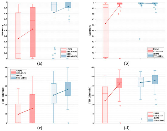
Figure 2.
Simulated online average spelling accuracy and average ITR (bits/min) for all participants on Datasets 1 and 2, applying the early stopping strategy. (a) Average spelling accuracy for Dataset 1; (b) average ITR for Dataset 1; (c) average spelling accuracy for Dataset 2; (d) average ITR for Dataset 2.
For Dataset 1, the inclusion of STE before UMM significantly improved both spelling accuracy and the information transfer rate (ITR) (accuracy: p = 0.046; ITR: p = 0.020). The average spelling accuracy increased from 35.49% to 52.23%, and the average ITR rose from 9.55 bits/min to 15.83 bits/min. When STE was applied before sDDM, both spelling accuracy and the ITR showed even greater improvements (accuracy: p = 0.004; ITR: p < 0.001). The average spelling accuracy increased from 81.62% to 92.56%, and the average ITR increased from 30.19 bits/min to 36.27 bits/min.
For Dataset 2, applying STE before UMM resulted in significant improvements in both spelling accuracy and the ITR (accuracy and ITR: p < 0.001). The average spelling accuracy increased from 62.88% to 95.76%, and the average ITR increased from 23.92 bits/min to 41.98 bits/min. However, compared to Dataset 1, the recording conditions or inherent signal properties of Dataset 2 may have contributed to improved classification performance. As a result, sDDM already achieved a high accuracy (97.99%) in Dataset 2, leaving little room for further improvement after applying STE (98.77%). Nonetheless, the ITR performance still showed a significant increase (ITR: p < 0.001), with the average ITR rising from 43.52 bits/min to 45.62 bits/min.
Furthermore, the relationship between UMM and sDDM was observed. In both datasets, sDDM consistently outperformed UMM under the same conditions, whether or not STE was used (Dataset 1 and 2, UMM vs. sDDM and STE-UMM vs. STE-sDDM, accuracy, and ITR: p < 0.001). The average and median spelling accuracy and the ITR of STE-sDDM were consistently the highest among the four methods shown in the legend.
Notably, in both datasets, there were participants with an ITR close to zero (i.e., spelling accuracy close to or below chance level). This phenomenon, commonly observed in some unsupervised algorithms, is referred to as pseudo-label contamination. It primarily occurs when excessive errors in pseudo-labels during online updates cause the classifier to fail [30]. For these participants, STE-sDDM successfully filtered out such cases in Dataset 2, whereas only one affected participant was identified in Dataset 1. This suggests that the denoising capability provided by STE improves early classification accuracy, thereby enhancing the reliability of pseudo-labels and significantly mitigating the issue of pseudo-label contamination.
Additionally, we further analyzed the average number of rounds used per trial for each participant under the early stopping strategy, as shown in Table 1. The average number of rounds for STE-sDDM was significantly lower than that of the other three methods (p < 0.001), demonstrating its significant role in enhancing communication speed.

Table 1.
The average number of rounds used by participants in a trial in the simulated online experiments with the early stopping strategy applied on Datasets 1 and 2.
5. Analysis and Discussion
5.1. Performance with Fixed Number of Rounds
The performance with early stopping reflects the ability of these classifiers to provide rapid and stable decisions in an online environment. To evaluate how they perform under various conditions, we assessed the ITR of EM, UMM, and sDDM, both with and without STE, using different fixed numbers of rounds, as shown in Figure 3.
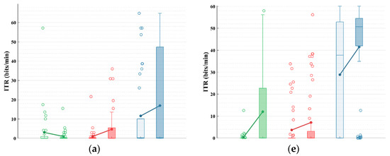
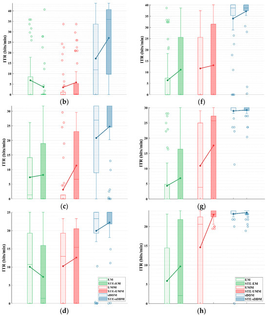
Figure 3.
Simulated online average ITRs (bits/min) for all participants in Datasets 1 and 2, using fixed and different rounds. The upper limit of the vertical axis represents the maximum possible ITR. (a–d) Average ITRs with fixed rounds of 2–5 for Dataset 1; (e–h) average ITRs with fixed rounds of 2–5 for Dataset 2.
As shown in Figure 3, after applying STE, the EM algorithm does not show a consistent improvement in Dataset 1. However, both UMM and sDDM show increases in the average ITR across all fixed rounds in both datasets. Furthermore, STE-sDDM consistently achieves the highest average ITR across all fixed rounds in both datasets.
We also analyzed the cumulative ITR curves for EM, UMM, and sDDM before and after applying STE, as shown in Figure 4.
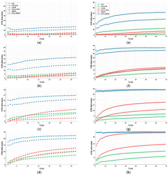
Figure 4.
Simulated online average cumulative ITR (bits/min) curves for all participants in Datasets 1 and 2 using fixed and different rounds. The horizontal axis represents the current average ITR across all tests after the current test, and the upper limit of the vertical axis represents the maximum possible ITR. (a–d) Average cumulative ITR curves for fixed 2–5 rounds on Dataset 1; (e–h) average cumulative ITR curves for fixed 2–5 rounds on Dataset 2.
As the number of trials increases, the unsupervised methods gradually learn more reliable classification models, resulting in an upward trend in the average cumulative ITR. In Dataset 2, when using five fixed rounds (as shown in Figure 4h), both STE-sDDM and sDDM approach the highest ITR levels allowed by their respective paradigms. In all other conditions, the average cumulative ITR of STE-sDDM consistently outperforms that of sDDM. Additionally, in both datasets, methods based on the sDDM classifier consistently yield a higher average cumulative ITR compared to other methods, especially in the initial trials, where they demonstrate superior performance and achieve usable classification results with fewer rounds than other classifiers.
5.2. Static vs. Dynamic Spatio-Temporal Equalizer Architectures
As mentioned earlier, while the spatio-temporal equalizer (STE) removes portions of background noise, it may also eliminate overlapping event-related components, resulting in ERP features in the output signal that differ from those in the original signal. Consequently, as the STE itself varies, the ERP features in the output signal may also exhibit different characteristics. To address this, we combined a static spatio-temporal equalizer with the sDDM algorithm to ensure that the ERP features in each input remain stable. However, for a spatio-temporal equalizer, the stability of background noise is only maintained in the short term. The background noise, , must be sufficiently close in time to the signal to ensure that spontaneous brain activity, electrode impedance, and other unrelated conditions remain relatively unchanged, thus preserving the assumption that and share the same spatio-temporal correlation. To balance these two considerations, we explored two variations in the STE-sDDM architecture: one using static noise and another using dynamic noise to design the spatio-temporal equalizer.
The architecture shown in Figure 5a uses the noise from the first trial as a single static spatio-temporal equalizer throughout the entire online process. Since this noise is collected before any stimulus events, it represents clean background noise without contamination from ERPs. In contrast, the architecture shown in Figure 5b collects new noise before each trial to create a dynamic spatio-temporal equalizer. Starting from the second trial, the time window of the noise overlaps with that of the previous trial, meaning that it contains event-related components (in most paradigms, including the two datasets used in this study, the time interval between trials is too short for noise without event-related components to be used for designing the spatio-temporal equalizer). To address this, we need to estimate the event-related components based on the sDDM classifier’s output and remove those components from the noise that are likely to correspond to the target stimulus before using it for the equalizer design.
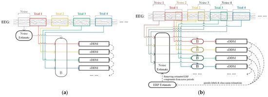
Figure 5.
Comparison of two algorithm architectures. (a) Static spatio-temporal equalization-sDDM using static noise to design the spatio-temporal equalizer; (b) dynamic spatio-temporal equalization-sDDM using dynamic noise to design the spatio-temporal equalizer.
In Figure 6, we show the learning curves for the two STE-sDDM architectures, with static and dynamic spatio-temporal equalizers, as well as the results for the sDDM algorithm without any equalizer, using Datasets 1 and 2. The fixed five-round data were used in this experiment to prevent the noise periods from contaminating the segments that should be removed due to overlap with prior trials.
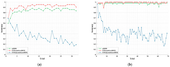
Figure 6.
Learning curves for static and dynamic spatio-temporal equalizers as well as the case without any spatio-temporal equalizer. The green curve represents sDDM without spatio-temporal equalization, the red curve represents the static spatio-temporal equalizer, and the blue curve represents the dynamic spatio-temporal equalizer. (a) Average spelling accuracy curve using a fixed 5 rounds for Dataset 1; (b) average spelling accuracy curve using a fixed 5 rounds for Dataset 2.
As shown in Figure 6a,b, the dynamic spatio-temporal equalizer leads to significant issues: Starting from the second trial, after the equalizer is updated, the stability assumption of the ERP features is disrupted, which significantly impacts classification performance. While the accuracy eventually stabilizes near a certain level, indicating that some common features between the changing ERPs are still captured by the sDDM classifier for a subset of participants, the negative impact of unstable ERP features clearly outweighs the benefit of the changing spatio-temporal correlation in the noise. Moreover, classification errors lead to inaccurate ERP feature estimates, which cause the dynamic equalizer to use noise containing more components related to the true ERP, further degrading its performance. This forms a vicious cycle where pseudo-label contamination reduces classifier performance. In contrast, the static spatio-temporal equalizer consistently outperforms the case without any equalization. While shifts in background noise properties may reduce the denoising efficiency of STE over time, the early improvement in classification accuracy is sufficient to ensure that STE-sDDM maintains superior performance over sDDM throughout the entire experiment.
5.3. Evaluation and Selection of the Required Noise Length for the Spatio-Temporal Equalizer
One of the advantages of unsupervised classification algorithms over supervised ones is the elimination of the calibration phase. However, if the noise duration required for the STE is too long, it would undoubtedly undermine the benefit of unsupervised methods. A 60 s calibration phase corresponds to approximately 300 training epochs, under which a supervised method can already develop a relatively reliable classification model. Figure 7 shows the performance of STE-sDDM in terms of the ITR after applying different noise lengths. The early stop strategy was applied. To plot the performance variation curve of STE-sDDM as noise length increases from 0 to 60 s, we selected the background noise durations of 1, 2, 5, 15, 30, 45, and 60 s prior to the start of trial 1.
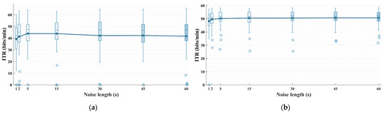
Figure 7.
Simulated online average ITR (bits/min) for all participants applying the early stop strategy using different noise signal lengths on Datasets 1 and 2. The upper limit of the vertical axis represents the maximum possible ITR. (a) Dataset 1; (b) Dataset 2.
When the noise duration was between 1 s and 5 s, the average ITR of STE-sDDM increased steadily. However, as the noise length increased from 5 s to 60 s, the average ITR remained nearly unchanged on Dataset 2 and even declined on Dataset 1. This decline may once again be attributed to changes in the spatio-temporal correlations of background noise. Additionally, a 5 s duration is significantly shorter than typical calibration phases, and it does not require participants to perform any extra tasks, thus not imposing any psychological or physiological burden on them. This duration can easily be integrated into the preparation phase of the paradigm (in fact, neither of the two datasets used in this study included a dedicated calibration phase for background noise collection before data acquisition). Therefore, the optimal noise duration for STE-sDDM is approximately 5 s.
6. Conclusions
This work presents an unsupervised online ERP classification algorithm, STE-sDDM, which builds upon the novel classification algorithm, sDDM. By utilizing STE, the algorithm removes spatio-temporal correlations in EEG background noise, reducing interference from colored noise on task-relevant components. This enhancement allows the sDDM to more accurately capture the class differences, thereby improving classification performance. We validated the superiority of combining STE with sDDM across two datasets with a total of 96 participants. The results demonstrate that, whether using fixed repetitions or an early stop strategy, the new method achieves the best classification accuracy and communication speed, outperforming not only sDDM but also EM and UMM, as well as their combinations with STE. Furthermore, we found that employing a static spatio-temporal equalizer helps maintain the consistency of classification features, thereby improving the integration of STE with unsupervised online classification methods. With the introduction of this novel unsupervised classification approach, BCI systems for human–machine interaction can achieve more reliable, faster, and plug-and-play online real-time control for external devices such as robotic hands, drones, and exoskeletons.
Author Contributions
Conceptualization, H.W. and X.H.; methodology, H.W.; software, H.W. and X.H.; formal analysis, H.W.; investigation, H.W. and X.H.; data curation, H.W.; writing—original draft preparation, H.W.; writing—review and editing, H.W. and S.L.; supervision, J.J., S.L. and A.C.; project administration, J.J.; funding acquisition, J.J. All authors have read and agreed to the published version of the manuscript.
Funding
This work was supported by the Grant National Natural Science Foundation of China under Grant 62176090 and STI 2030-major projects 2022ZD0208900; in part by Shanghai Municipal Science and Technology Major Project under Grant 2021SHZDZX; and by the Project of Jiangsu Province Science and Technology Plan Special Fund in 2022 (Key research and development plan industry foresight, fundamental research fund for the central universities JKH01231636 and key core technologies) under Grant BE2022064-1.
Institutional Review Board Statement
This work involved human subjects or animals in its research. Approval of all ethical and experimental procedures and protocols was granted by the Bioethics Committee of East China University of Science and Technology, Shanghai, China.
Informed Consent Statement
Informed consent was obtained from all subjects involved in the study.
Data Availability Statement
The publicly available datasets used in this study can be accessed at http://gigadb.org/dataset/100542 (accessed on 26 June 2024). For access to additional data, please contact the corresponding author.
Acknowledgments
The authors would like to thank the users who took part in this study.
Conflicts of Interest
The authors declare no conflicts of interest.
References
- Gao, S.; Wang, Y.; Gao, X.; Hong, B. Visual and Auditory Brain–Computer Interfaces. IEEE Trans. Biomed. Eng. 2014, 61, 1436–1447. [Google Scholar] [CrossRef] [PubMed]
- Zhang, H.; Guan, C.; Wang, C. Asynchronous P300-Based Brain–Computer Interfaces: A Computational Approach with Statistical Models. IEEE Trans. Biomed. Eng. 2008, 55, 1754–1763. [Google Scholar] [CrossRef] [PubMed]
- Xu, S.; Liu, Y.; Lee, H.; Li, W. Neural Interfaces: Bridging the Brain to the World beyond Healthcare. Exploration 2024, 4, 20230146. [Google Scholar] [CrossRef]
- Vangi, M.; Brogi, C.; Topini, A.; Secciani, N.; Ridolfi, A. Enhancing sEMG-Based Finger Motion Prediction with CNN-LSTM Regressors for Controlling a Hand Exoskeleton. Machines 2023, 11, 747. [Google Scholar] [CrossRef]
- Borboni, A.; Elamvazuthi, I.; Cusano, N. EEG-Based Empathic Safe Cobot. Machines 2022, 10, 603. [Google Scholar] [CrossRef]
- Dmytriyev, Y.; Insero, F.; Carnevale, M.; Giberti, H. Brain–Computer Interface and Hand-Guiding Control in a Human–Robot Collaborative Assembly Task. Machines 2022, 10, 654. [Google Scholar] [CrossRef]
- Xiao, X.; Xu, M.; Jin, J.; Wang, Y.; Jung, T.-P.; Ming, D. Discriminative Canonical Pattern Matching for Single-Trial Classification of ERP Components. IEEE Trans. Biomed. Eng. 2020, 67, 2266–2275. [Google Scholar] [CrossRef]
- Rezeika, A.; Benda, M.; Stawicki, P.; Gembler, F.; Saboor, A.; Volosyak, I. Brain–Computer Interface Spellers: A Review. Brain Sci. 2018, 8, 57. [Google Scholar] [CrossRef]
- Kübler, A. The History of BCI: From a Vision for the Future to Real Support for Personhood in People with Locked-in Syndrome. Neuroethics 2020, 13, 163–180. [Google Scholar] [CrossRef]
- Jin, J.; Chen, Z.; Xu, R.; Miao, Y.; Wang, X.; Jung, T.-P. Developing a Novel Tactile P300 Brain-Computer Interface with a Cheeks-Stim Paradigm. IEEE Trans. Biomed. Eng. 2020, 67, 2585–2593. [Google Scholar] [CrossRef]
- Farwell, L.A.; Donchin, E. Talking off the Top of Your Head: Toward a Mental Prosthesis Utilizing Event-Related Brain Potentials. Electroencephalogr. Clin. Neurophysiol. 1988, 70, 510–523. [Google Scholar] [CrossRef]
- Aggarwal, S.; Chugh, N. Review of Machine Learning Techniques for EEG Based Brain Computer Interface. Arch. Comput. Methods Eng. 2022, 29, 3001–3020. [Google Scholar] [CrossRef]
- Krusienski, D.J.; Sellers, E.W.; McFarland, D.J.; Vaughan, T.M.; Wolpaw, J.R. Toward Enhanced P300 Speller Performance. J. Neurosci. Methods 2008, 167, 15–21. [Google Scholar] [CrossRef] [PubMed]
- Hoffmann, U.; Vesin, J.-M.; Ebrahimi, T.; Diserens, K. An Efficient P300-Based Brain–Computer Interface for Disabled Subjects. J. Neurosci. Methods 2008, 167, 115–125. [Google Scholar] [CrossRef]
- Sosulski, J.; Tangermann, M. Introducing Block-Toeplitz Covariance Matrices to Remaster Linear Discriminant Analysis for Event-Related Potential Brain–Computer Interfaces. J. Neural Eng. 2022, 19, 066001. [Google Scholar] [CrossRef]
- Lawhern, V.J.; Solon, A.J.; Waytowich, N.R.; Gordon, S.M.; Hung, C.P.; Lance, B.J. EEGNet: A Compact Convolutional Neural Network for EEG-Based Brain–Computer Interfaces. J. Neural Eng. 2018, 15, 056013. [Google Scholar] [CrossRef]
- Schirrmeister, R.T.; Springenberg, J.T.; Fiederer, L.D.J.; Glasstetter, M.; Eggensperger, K.; Tangermann, M.; Hutter, F.; Burgard, W.; Ball, T. Deep Learning with Convolutional Neural Networks for EEG Decoding and Visualization. Hum. Brain Mapp. 2017, 38, 5391–5420. [Google Scholar] [CrossRef]
- Wang, Z.; Chen, C.; Li, J.; Wan, F.; Sun, Y.; Wang, H. ST-CapsNet: Linking Spatial and Temporal Attention with Capsule Network for P300 Detection Improvement. IEEE Trans. Neural Syst. Rehabil. Eng. 2023, 31, 991–1000. [Google Scholar] [CrossRef]
- Jin, J.; Sellers, E.W.; Zhang, Y.; Daly, I.; Wang, X.; Cichocki, A. Whether Generic Model Works for Rapid ERP-Based BCI Calibration. J. Neurosci. Methods 2013, 212, 94–99. [Google Scholar] [CrossRef]
- Zhao, Y.; Wang, Z.; Zhang, Z.; Liu, J.; Chen, L.; Qi, H.; Jiao, X.; He, F.; Zhou, P.; Ming, D. A Transplantation of Subject-Independent Model in Cross-Platform BCI. Int. J. Mach. Learn. Cyber. 2018, 9, 959–967. [Google Scholar] [CrossRef]
- Jin, J.; Li, S.; Daly, I.; Miao, Y.; Liu, C.; Wang, X.; Cichocki, A. The Study of Generic Model Set for Reducing Calibration Time in P300-Based Brain–Computer Interface. IEEE Trans. Neural Syst. Rehabil. Eng. 2020, 28, 3–12. [Google Scholar] [CrossRef]
- Gao, W.; Huang, W.; Li, M.; Gu, Z.; Pan, J.; Yu, T.; Yu, Z.L.; Li, Y. Eliminating or Shortening the Calibration for a P300 Brain–Computer Interface Based on a Convolutional Neural Network and Big Electroencephalography Data: An Online Study. IEEE Trans. Neural Syst. Rehabil. Eng. 2023, 31, 1754–1763. [Google Scholar] [CrossRef]
- Li, Y.; Guan, C.; Li, H.; Chin, Z. A Self-Training Semi-Supervised SVM Algorithm and Its Application in an EEG-Based Brain Computer Interface Speller System. Pattern Recognit. Lett. 2008, 29, 1285–1294. [Google Scholar] [CrossRef]
- Wu, D. Active Semi-Supervised Transfer Learning (ASTL) for Offline BCI Calibration. In Proceedings of the 2017 IEEE International Conference on Systems, Man, and Cybernetics (SMC), Banff, Canada, 5–8 October 2017; pp. 246–251. [Google Scholar]
- Ogino, M.; Kanoga, S.; Ito, S.-I.; Mitsukura, Y. Semi-Supervised Learning for Auditory Event-Related Potential-Based Brain–Computer Interface. IEEE Access 2021, 9, 47008–47023. [Google Scholar] [CrossRef]
- Kindermans, P.-J.; Verstraeten, D.; Schrauwen, B. A Bayesian Model for Exploiting Application Constraints to Enable Unsupervised Training of a P300-Based BCI. PLoS ONE 2012, 7, e33758. [Google Scholar] [CrossRef]
- Hubner, D.; Verhoeven, T.; Muller, K.-R.; Kindermans, P.-J.; Tangermann, M. Unsupervised Learning for Brain-Computer Interfaces Based on Event-Related Potentials: Review and Online Comparison [Research Frontier]. IEEE Comput. Intell. Mag. 2018, 13, 66–77. [Google Scholar] [CrossRef]
- Hübner, D.; Verhoeven, T.; Schmid, K.; Müller, K.-R.; Tangermann, M.; Kindermans, P.-J. Learning from Label Proportions in Brain-Computer Interfaces: Online Unsupervised Learning with Guarantees. PLoS ONE 2017, 12, e0175856. [Google Scholar] [CrossRef]
- Verhoeven, T.; Hübner, D.; Tangermann, M.; Müller, K.R.; Dambre, J.; Kindermans, P.J. Improving Zero-Training Brain-Computer Interfaces by Mixing Model Estimators. J. Neural Eng. 2017, 14, 036021. [Google Scholar] [CrossRef]
- Sosulski, J.; Tangermann, M. UMM: Unsupervised Mean-Difference Maximization. arXiv 2023, arXiv:2306.11830. [Google Scholar]
- Paris, A.; Vosoughi, A.; Atia, G. Whitening 1/f-Type Noise in Electroencephalogram Signals for Steady-State Visual Evoked Potential Brain-Computer Interfaces. In Proceedings of the 2014 48th Asilomar Conference on Signals, Systems and Computers, Pacific Grove, CA, USA, 2–5 November 2014; pp. 204–207. [Google Scholar]
- He, B.J. Scale-Free Brain Activity: Past, Present, and Future. Trends Cogn. Sci. 2014, 18, 480–487. [Google Scholar] [CrossRef]
- Baillet, S.; Mosher, J.C.; Leahy, R.M. Electromagnetic Brain Mapping. IEEE Signal Process. Mag. 2001, 18, 14–30. [Google Scholar] [CrossRef]
- Britten, K.H.; Shadlen, M.N.; Newsome, W.T.; Movshon, J.A. The Analysis of Visual Motion: A Comparison of Neuronal and Psychophysical Performance. J. Neurosci. 1992, 12, 4745–4765. [Google Scholar] [CrossRef]
- Yang, C.; Han, X.; Wang, Y.; Saab, R.; Gao, S.; Gao, X. A Dynamic Window Recognition Algorithm for SSVEP-Based Brain-Computer Interfaces Using a Spatio-Temporal Equalizer. Int. J. Neural Syst. 2018, 28, 1850028. [Google Scholar] [CrossRef] [PubMed]
- Yang, C.; Zhang, H.; Zhang, S.; Han, X.; Gao, S.; Gao, X. The Spatio-Temporal Equalization for Evoked or Event-Related Potential Detection in Multichannel EEG Data. IEEE Trans. Biomed. Eng. 2020, 67, 2397–2414. [Google Scholar] [CrossRef]
- Jin, J.; He, X.; Allison, B.Z.; Qin, K.; Wang, X.; Cichocki, A. Leveraging Spatiotemporal Estimation for Online Adaptive Steady-State Visual Evoked Potential Recognition. IEEE Trans. Cogn. Dev. Syst. 2024, 16, 1943–1954. [Google Scholar] [CrossRef]
- Akaike, H. Autoregressive Model Fitting for Control. Ann. Inst. Stat. Math. 1971, 23, 163–180. [Google Scholar] [CrossRef]
- Schwarz, G. Estimating the Dimension of a Model. Ann. Stat. 1978, 6, 461–464. [Google Scholar]
- Jin, J.; Allison, B.Z.; Sellers, E.W.; Brunner, C.; Horki, P.; Wang, X.; Neuper, C. Optimized Stimulus Presentation Patterns for an Event-Related Potential EEG-Based Brain–Computer Interface. Med. Biol. Eng. Comput. 2011, 49, 181–191. [Google Scholar] [CrossRef]
- Lee, M.-H.; Kwon, O.-Y.; Kim, Y.-J.; Kim, H.-K.; Lee, Y.-E.; Williamson, J.; Fazli, S.; Lee, S.-W. EEG Dataset and OpenBMI Toolbox for Three BCI Paradigms: An Investigation into BCI Illiteracy. GigaScience 2019, 8, giz002. [Google Scholar] [CrossRef]
- Yeom, S.-K.; Fazli, S.; Müller, K.-R.; Lee, S.-W. An Efficient ERP-Based Brain-Computer Interface Using Random Set Presentation and Face Familiarity. PLoS ONE 2014, 9, e111157. [Google Scholar] [CrossRef]


Disclaimer/Publisher’s Note: The statements, opinions and data contained in all publications are solely those of the individual author(s) and contributor(s) and not of MDPI and/or the editor(s). MDPI and/or the editor(s) disclaim responsibility for any injury to people or property resulting from any ideas, methods, instructions or products referred to in the content. |
© 2025 by the authors. Licensee MDPI, Basel, Switzerland. This article is an open access article distributed under the terms and conditions of the Creative Commons Attribution (CC BY) license (https://creativecommons.org/licenses/by/4.0/).