Rolling Bearing Fault Diagnosis Based on Wavelet Overlapping Group Shrinkage and Extended Envelope Hierarchical Multiscale-Weighted Permutation Entropy

Abstract

Rolling bearing vibration signals contain rich fault feature information. However, their periodic pulse feature is often interfered with by strong background noise, which reduces the feature recognition ability of fault diagnosis strategies. Therefore, accurately extracting periodic pulse information under strong background noise is a key challenge in rolling bearing fault diagnosis. To address this, a fault feature extraction strategy combining wavelet overlapping group shrinkage (WOGS) and extended enveloped hierarchical multiscale-weighted permutation entropy (EEHMWPE) is proposed. First, wavelet decomposition is applied to decompose original vibration signals into wavelet coefficients, with WOGS adaptively adjusting the shrinkage level based on energy relationships to effectively suppress noise. Next, for the denoised signal, EEHMWPE extracts periodic pulse features by integrating envelope analysis, weighting, and extended statistical features. Envelope processing enhances fault-induced impulses, the weighting scheme highlights dominant fault patterns, and extended statistical features further improve the class separability between normal and fault signals. Finally, the strategy was validated on the bearing test bench, CWRU, and HUST datasets, all of which achieved over 99% accuracy with superior feature recognition.

1. Introduction

Rolling bearings are essential components in rotating machinery often exposed to high-speed operations and localized stresses that may result in operational failures. Consequently, the regular monitoring of bearing health to prevent severe damage has garnered significant attention among researchers [1]. However, practical operating environments are often compromised by intense background noise, attributable to equipment instability, environmental fluctuations, and electromagnetic disturbances [2,3]. These disturbances cause the collected data to deviate from actual values, masking meaningful fault characteristics and thereby increasing the complexity of bearing fault diagnosis (BFD) [4]. Therefore, a key challenge in BFD is developing denoising and feature extraction techniques that can effectively extract transient fault pulses from noise-contaminated signals, ensuring accurate and reliable fault identification.

Over the years, significant efforts have been devoted to reducing noise interference and extracting meaningful fault features [5,6,7]. Various signal denoising techniques have been explored, including empirical mode decomposition (EMD) [8,9], variational mode decomposition (VMD) [10,11], and wavelet transform (WT) [12,13]. While EMD decomposes signals into intrinsic mode functions (IMFs) for denoising but may suffer from mode mixing, where IMFs contain mixed frequencies, especially when noise overlaps with useful signals. VMD decomposes signals into sparsity-based modes but requires predefined mode numbers and is noise-sensitive. WT performs multiscale decomposition, removing high-frequency noise while preserving low- or mid-frequency signals, enabling effective denoising. Donoho et al. 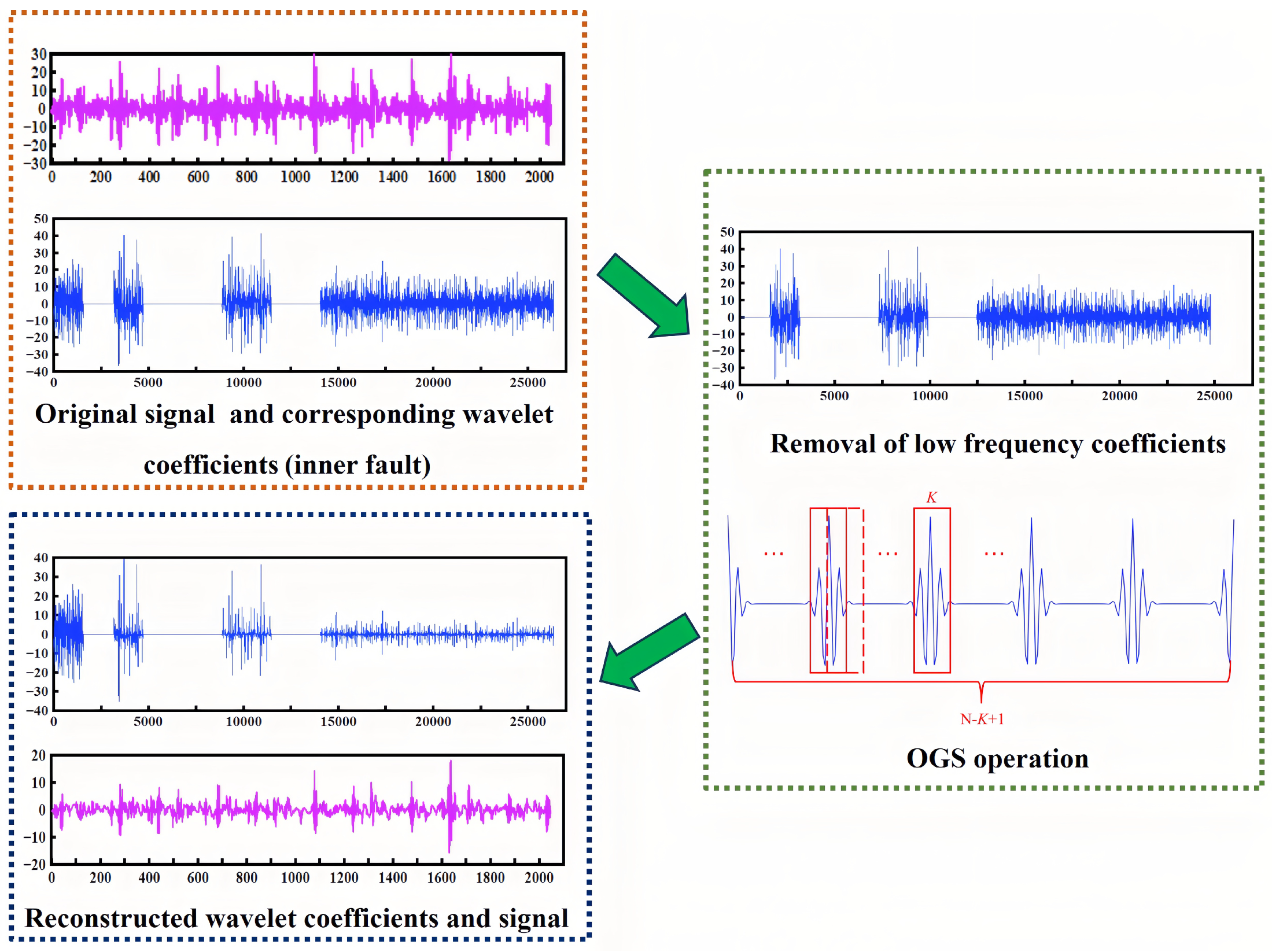[14] combined the soft thresholding technique with wavelet transform, effectively removing noise components with wavelet coefficients smaller than the threshold while preserving the main features of the signal. However, wavelet thresholding methods overlook signal sparsity. To enhance sparsity, Selesnick et al. [15] proposed the overlapping group shrinkage (OGS) method, which achieves promising results for group-sparse signals. Wang et al. [16] applied OGS in fractional spline wavelet domains for bearing fault signal extraction. Zhao et al. [17] used OGS with shift-invariant wavelet transforms for electrocardiogram denoising. OGS has been successfully applied to bearing fault diagnosis due to the group-sparse nature of wavelet coefficients [18,19]. The OGS relies on prior statistical models, such as Gaussian or Laplace distributions, and it requires detailed statistical analysis and parameter estimation for each wavelet coefficient. This dependence on statistical modeling introduces prior assumptions and computational complexity. To address these issues, this paper proposes a WOGS method, which is crucial for overcoming the challenge of strong background noise in fault diagnosis. WOGS directly adjusts the shrinkage parameters based on the $L2$ norms energy relationships at the group level without prior modeling assumptions, thus reducing computational complexity. It effectively preserves key high-frequency information related to periodic event extraction, improving denoising performance.

After denoising, feature extraction from bearing vibration signals is a key step in fault diagnosis [20]. Periodic pulse information often serves as a crucial indicator of fault characteristics, and the ability to accurately extract these features directly determines the effectiveness of the final diagnosis. However, bearing vibration signals are complex, which makes it difficult to directly extract fault information. As a key parameter in mechanical dynamics, entropy features can characterize the modal periodicity and the orderliness, or disorderliness, of pulse sequences in faulty bearing vibration signals. Civera et al. [21] proposed instantaneous spectral entropy (ISE) and continuous wavelet transform for anomaly detection and fault diagnosis, in which ISE is highlighted as being particularly sensitive to fault signals and potentially suitable for real-time monitoring. Zhuang et al. [22] proposed a feature extraction method based on VMD and sample entropy (SE), where SE quantifies the probability of changes in the time series due to variations in data positions, effectively capturing the characteristics of fault signals. Compared to ISE, which struggles to characterize system nonlinearity, and SE, which is unstable for short sequences, PE is widely used in BFD due to its simplicity and sensitivity to regular impulses, effectively measuring randomness and capturing signal fluctuations [23]. However, PE only analyzes single-scale time series and cannot assess fault information in complex signals. To address this, Bie et al. [24] proposed multiscale permutation entropy (MPE) to extract periodic pulse features from bearing fault signals. However, MPE overlooks fault information in high-frequency components. Li et al. [25] introduced hierarchical permutation entropy (HPE) to separate low- and high-frequency components, enhancing fault information extraction. However, HPE may lead to information loss. Yang et al. [26] proposed hierarchical multiscale permutation entropy (HMPE), combining hierarchical and multiscale coarse-graining strategies. Wan et al. 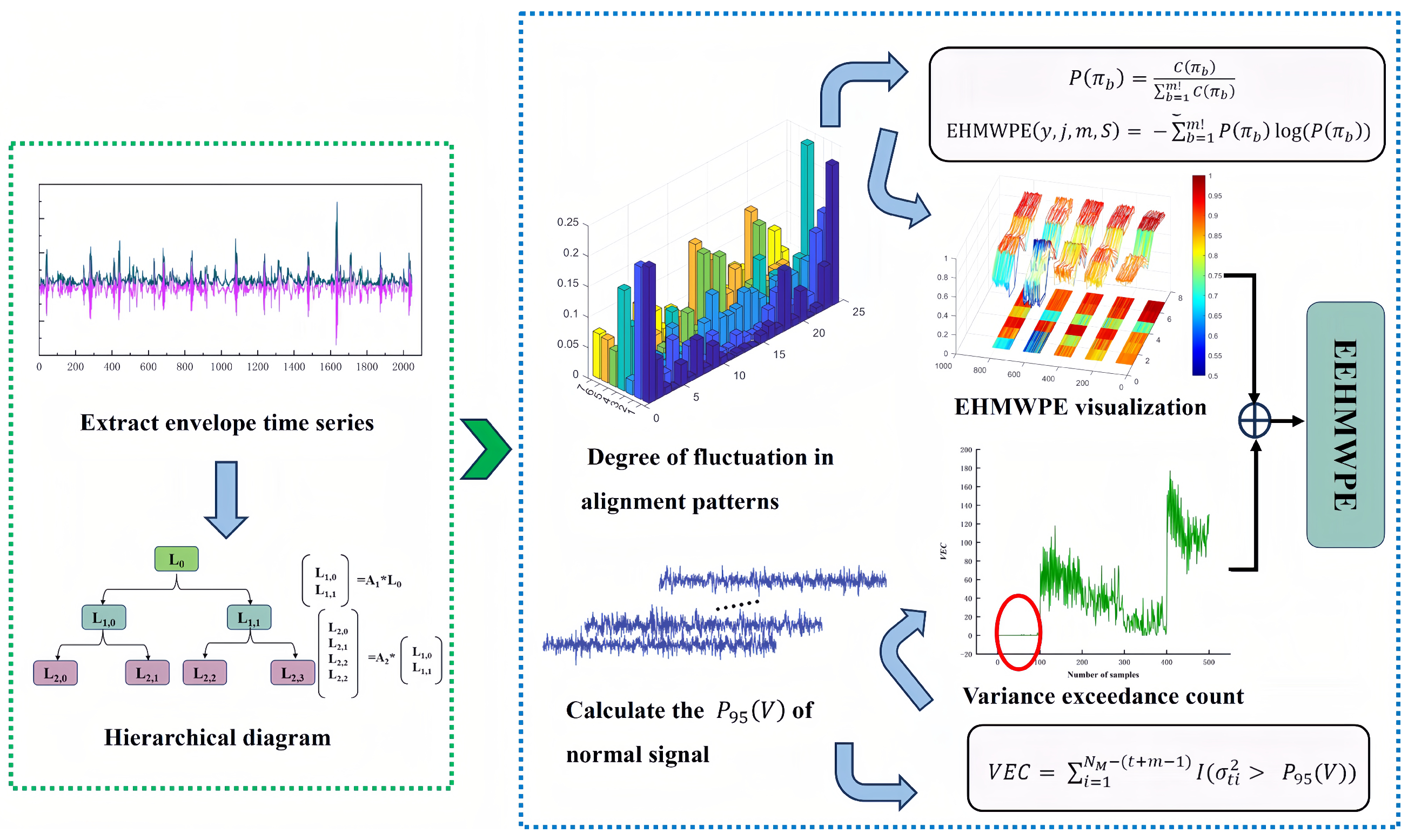[27] used multiscale-weighted permutation entropy (MWPE) to represent periodic pulses in wind turbine bearings and local linear embedding for degradation analysis. However, HMPE and MWPE do not fully consider class separability, which may impact feature discrimination and diagnostic accuracy. Additionally, envelope signals, rich in pulse information, enhance fault feature changes and improve fault recognition reliability [28]. This paper proposes an EEHMWPE feature vector, combining enveloped hierarchical multiscale-weighted permutation entropy (EHMWPE) with extended statistical features. The EEHMWPE based on envelope signals considers the probability of the same pattern with different state vector amplitudes in coarse-grained time series, which improves upon HMPE’s limitations. Extended statistical features enhance EHMWPE’s robustness and class separability. Finally, a BFD strategy based on WOGS and EEHMWPE was applied to rolling bearing experimental datasets.

The innovative contributions of this article are as follows:

(1) A novel and efficient denoising method, WOGS, is proposed that adaptively adjusts the shrinkage level based on the energy relationships within wavelet coefficient groups. It retains normal signal information while enhancing the periodic pulse information from fault signals.

(2) A feature vector EEHMWPE was constructed to quantify the complexity of time series, effectively enhancing the inter-class distance between normal and faulty signals by integrating envelope information, weighting, and extended statistical features. It provides more discriminative features for classification models.

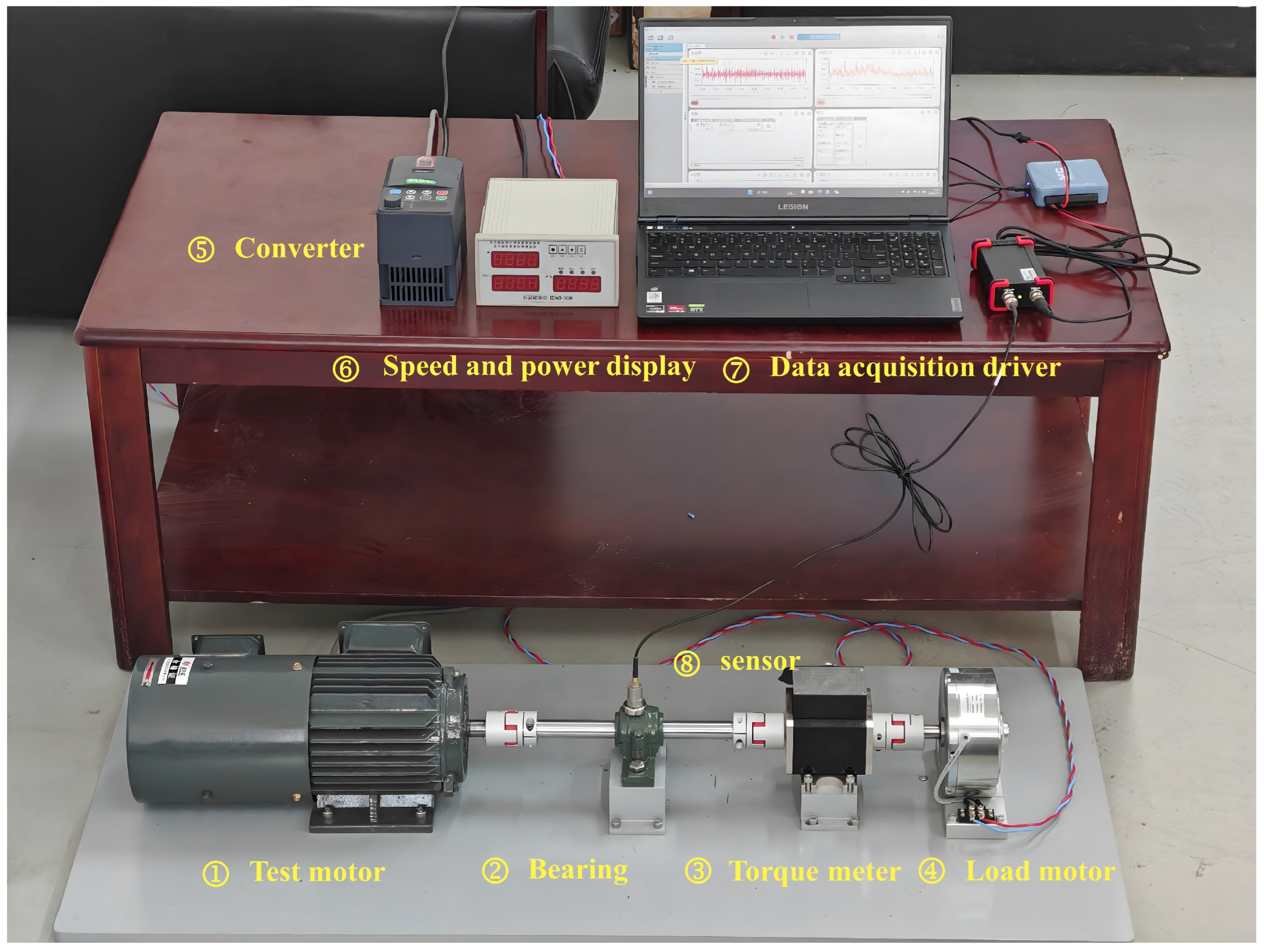
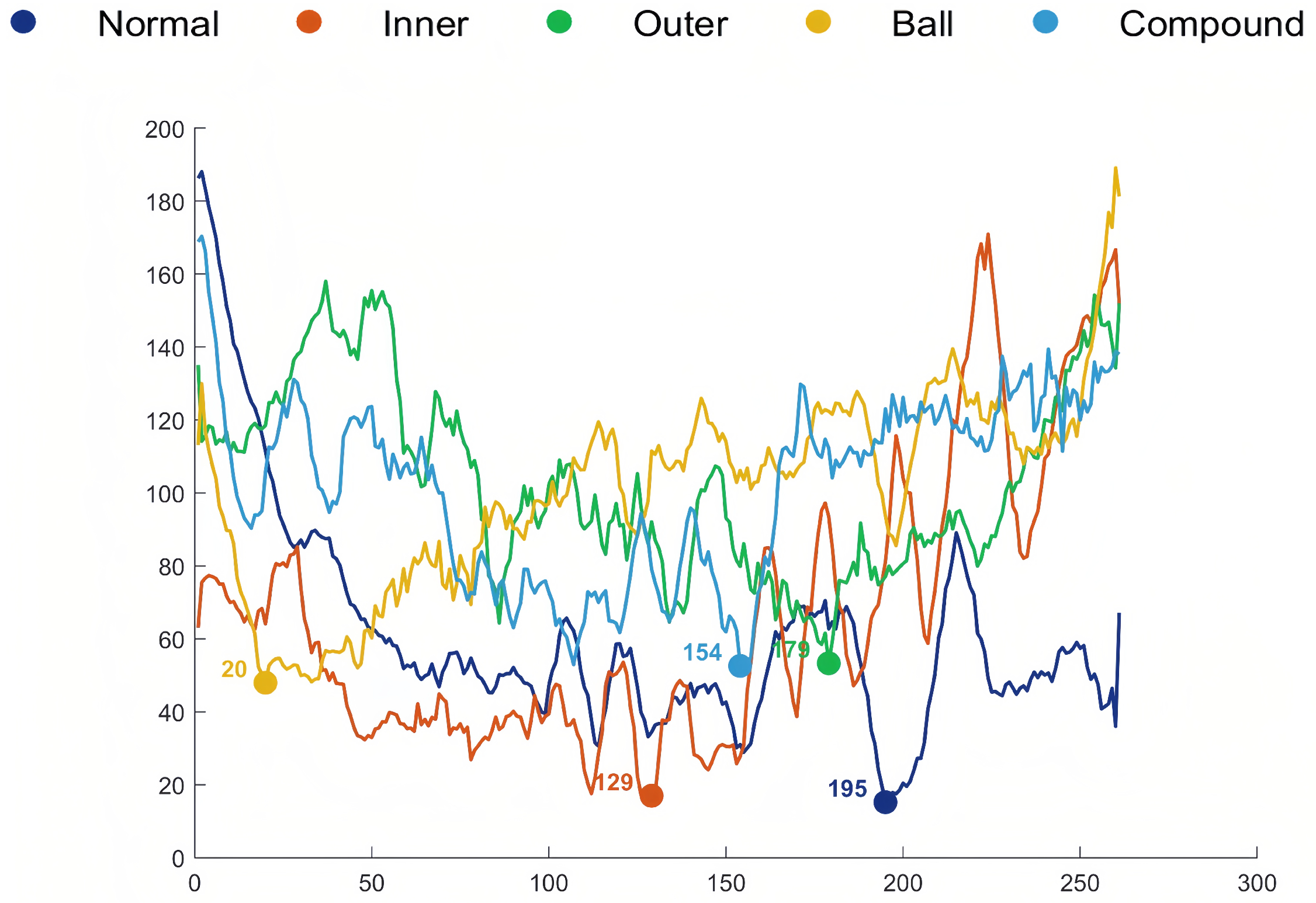
(3) The WOGS-EEHMWPE strategy’s advantages in feature extraction were validated using datasets from a bearing test rig and the CWRU dataset. Classification results with a standard classifier showed that the WOGS-denoised signals significantly enhance EEHMWPE’s feature extraction performance, with WOGS-EEHMWPE achieving the highest fault feature extraction capability.

The remainder of this article is organized as follows: Section 2 introduces the theoretical background of wavelet overlap shrinkage denoising and extended envelope layered multi-scale weighted permutation entropy. Section 3 provides a detailed introduction to the proposed WOGS denoising method and the EEHMWPE feature vector. Section 4 demonstrates the effectiveness of the proposed strategy through experiments. Section 5 further verified the performance of this strategy on the CWRU dataset and the HSUT dataset. Finally, Section 6 concludes the paper and discusses future directions.

2. Theoretical Background

2.1. Wavelet Overlap Group Shrinkage

In practical applications, bearing vibration signals often contain significant noise. The goal of denoising using wavelet thresholding is to separate the useful signal from the noise as effectively as possible. The specific process involves the following: (1) Selecting an appropriate wavelet basis to decompose the noisy signal and obtain wavelet coefficients; (2) processing the coefficients of each layer to obtain the reconstructed wavelet coefficients; and (3) applying the inverse transform to the reconstructed coefficients to obtain the denoised signal.

The denoising problem is addressed within the framework of a signal model:

$$x=y+\omega .$$

(1)

Here, x represents the noisy signal, y is the denoised signal, and $\omega$ denotes white Gaussian noise. The primary objective of the denoising method is to minimize the $\omega$ component in x. The hard and soft thresholding functions proposed by Donoho et al. [14] represent the noise component $\omega$ in the wavelet transform domain using a threshold $thr$. This is achieved by subtracting the threshold $thr$ from the wavelet coefficients to achieve denoising.

$$W_{z,c}=\mathcal{W}\left(x\right),$$

(2)

$${\widehat{W}}_{z,c}=\left\{\begin{array}{l}{W}_{z,c}\left|W_{z,c}\right|\ge thr\\ 0\left|W_{z,c}\right|<thr,\end{array}\right.$$

(3)

$${\widehat{W}}_{z,c}=\left\{\begin{array}{l}\left[sgn\left(W_{z,c}\right)\right]\left(\left|W_{z,c}-thr\right|\right)\left|W_{z,c}\right|\ge thr\\ 0\left|W_{z,c}\right|<thr.\end{array}\right.$$

(4)

Here, $\mathcal{W}(•)$ denotes the wavelet decomposition, and $W_{z,c}$ represents the wavelet coefficients (where z is the decomposition level and c is the order of the wavelet coefficients). Given a signal of length N, wavelet decomposition is performed to obtain the reconstructed wavelet coefficients ${\widehat{W}}_{z,c}$. An appropriate threshold $thr$ can be set as follows:

$$thr=\sigma \sqrt{2lnN}.$$

(5)

Here, $\sigma$ represents the standard deviation of the signal. Since the noise in the actual signal is unknown, it is necessary to estimate $\sigma$ using the following formula [29]:

$$\sigma =Median\left(\left|W_{1,c}\right|\right)/0.6745.$$

(6)

Here, $\left|•\right|$ denotes the absolute value of $W_{1,c}$, and $Median(•)$ represents the median of the sequence within the parentheses. Unlike the fixed threshold method, which estimates noise to determine a threshold, the core idea of the WOGS algorithm is to treat adjacent wavelet coefficients as a group. The number of sampling points $x_{u.K}$ in the u-th group is defined by the clustering point number K. The $L2$ norms ${∥x_{z,u.K}∥}_2$ of the wavelet coefficients in the z-th layer group is set as a dynamic weighting factor ${\gamma }_z$. A larger $L2$ norms of the wavelet group corresponds to significant fault features. The overlap property and ${\gamma }_z$ normalization factor facilitate a smooth transition of the ${∥x_{z,u.K}∥}_2$ energy between wavelet coefficient groups, ensuring continuity in energy variation.

$$x_{u.K}=\left[x\left(u\right),\dots ,x(u+K-1)\right]\in {\mathbb{R}}^K,$$

(7)

$${\gamma }_z={\displaystyle \frac{{∥x_{z,u.K}∥}_2-min\left({∥x_{z,u.K}∥}_2\right)}{max\left({∥x_{z,u.K}∥}_2\right)-min\left({∥x_{z,u.K}∥}_2\right)}},$$

(8)

$${\widehat{WO}}_{z,c}=W_{z,c}{\gamma }_z.$$

(9)

Here, ${\widehat{WO}}_{z,c}$ denotes the reconstructed wavelet coefficients, which reveal the energy relationship of the group and effectively enhance the distinguishability of impulse information in the signal. Additionally, the objective function for optimizing the clustering point number K is defined as follows [30]:

$$F\left(x\right)={\displaystyle \frac{1}{2}}{∥y-x∥}_2^2+{\displaystyle \frac{1}{2}}\sum _u\left({∥x_{u.K}∥}_2\right).$$

(10)

Here, ${\displaystyle \frac{1}{2}}{∥y-x∥}_2^2$ represents the data fitting term, which measures the preservation of the original signal; and ${\displaystyle \frac{1}{2}}{\displaystyle \sum _u}\left({∥x_{u.K}∥}_2\right)$ denotes the regularization term, which constrains the signal groups and promotes sparsity. The range of the number of clustering points K should theoretically be less than the fault impulse period T:

$$T={\displaystyle \frac{f_s}{f_o}}.$$

(11)

Here, $f_s$ is the sampling frequency, and $f_o$ represents the fault characteristic frequencies. Therefore, the range of K should be set as follows:

$$1\le K\le {\displaystyle \frac{f_s}{min\left(f_{BPFO},f_{BPFI},f_{BSF}\right)}}.$$

(12)

Here, $f_{BPFO}$, $f_{BPFI}$, and $f_{BSF}$ represent the fault characteristic frequencies of the outer faults, inner faults, and ball faults, respectively. Finally, the optimal K value is determined based on the objective function $F\left(x\right)$, after which the wavelet coefficient reconstruction is performed and the denoised signal y is obtained by applying the inverse wavelet transform ${\mathcal{W}}^{-1}(•)$:

$$y={\mathcal{W}}^{-1}\left({\widehat{WO}}_{z,c}\right).$$

(13)

2.2. Extended Envelope Hierarchical Multiscale-Weighted Permutation Entropy

The principle of EHMWPE is to perform hierarchical decomposition on the envelope time series of the denoised signal y, obtaining different components for analysis. The entropy value is then calculated based on the weighted information derived from the coarse-grained components. The specific process is as follows: For a given denoised signal time series $\left\{y\left(n\right),n=1,2\dots ,N\right\}$, the envelope signal $\tilde{y}$ is first obtained through Hilbert transform. Then, hierarchical processing is performed with j layers, yielding $2^j-1$ different component subsequences. The hierarchical operator is as follows:

$${\stackrel{\sim }{L}}_{0,0}=\stackrel{\sim }{y},$$

(14)

$${\stackrel{\sim }{L}}_{j,2k}\left(i\right)={\displaystyle \frac{{\stackrel{\sim }{L}}_{j-1,k}\left(2i+1\right)+{\stackrel{\sim }{L}}_{j-1,k}\left(2i+2\right)}{2}},i=0,1,\dots ,{\displaystyle \frac{N}{2^j}}-1,$$

(15)

$${\stackrel{\sim }{L}}_{j,2k+1}\left(i\right)={\displaystyle \frac{{\stackrel{\sim }{L}}_{j-1,k}\left(2i+1\right)-{\stackrel{\sim }{L}}_{j-1,k}\left(2i+2\right)}{2}},i=0,1,\dots ,{\displaystyle \frac{N}{2^j}}-1.$$

(16)

Here, ${\tilde{L}}_{j,2k}\left(i\right)$ and ${\tilde{L}}_{j,2k+1}\left(i\right)$ represent the moving average and moving difference of $\tilde{y}$, respectively; ${\tilde{L}}_{j,2k}\left(i\right)$ captures the long-term trend or global structure of the signal; while ${\tilde{L}}_{j,2k+1}\left(i\right)$ highlights local variations and emphasizes abrupt changes. The basic matrix form is as follows:

$$A=\left[\begin{array}{ccccccc}{\displaystyle \frac{1}{2}}& {\displaystyle \frac{1}{2}}& 0& 0& \cdots & 0& 0\\ 0& 0& {\displaystyle \frac{1}{2}}& {\displaystyle \frac{1}{2}}& \cdots & 0& 0\\ ⋮& ⋮& ⋮& ⋮& \ddots & ⋮& ⋮\\ {\displaystyle \frac{1}{2}}& -{\displaystyle \frac{1}{2}}& 0& 0& \cdots & 0& 0\\ 0& 0& {\displaystyle \frac{1}{2}}& -{\displaystyle \frac{1}{2}}& \cdots & 0& 0\\ ⋮& ⋮& ⋮& ⋮& \ddots & ⋮& ⋮\end{array}\right].$$

(17)

Further, we have the following:

$$A_j={\left[\begin{array}{ccc}{A}_{{\displaystyle \frac{N}{2^{j-1}}}}& \cdots & 0\\ ⋮& \ddots & ⋮\\ 0& \cdots & A_{{\displaystyle \frac{N}{2^{j-1}}}}\end{array}\right]}_{2^{j-1}\ast 2^{j-1}}.$$

(18)

Therefore, the following applies:

$$\left[\begin{array}{c}{\tilde{L}}_{j,0}\\ ⋮\\ {\tilde{L}}_{j,2^{j-1}}\end{array}\right]=A_j\ast A_{j-1}\dots \ast A_1{L}_{0,0}.$$

(19)

The coarse-grained component after decomposition can be expressed as follows:

$$M_{j,k}\left(S\right)={\displaystyle \frac{1}{S}}\sum _{i=\left(p-1\right)S+1}^{pS}{\stackrel{\sim }{L}}_{j,k}\left(i\right),p=1,2,\dots ,(N-j)/S.$$

(20)

Here, S denotes the scale factor, and the length of $M_{j,k}$ is $N_M$. For each window $M_t,M_{t+1},\dots M_{t+m-1}$ in the time series $M_{j,k}$, where the window length is the embedding scale m, the variance ${\sigma }_t^2$ of the window is calculated as follows:

$${\sigma }_t^2={\displaystyle \frac{1}{m}}\sum _{i=0}^{m-1}{\left(M_{t+i}-{\stackrel{-}{M}}_t\right)}^2,$$

(21)

$${\stackrel{-}{M}}_t={\displaystyle \frac{1}{m}}\sum _{i=0}^{m-1}{M}_{t+i}.$$

(22)

Here, ${\overline{M}}_t$ is the mean of all the data points in the window. The variance ${\sigma }_t^2$ of each window is then matched with the window’s arrangement pattern ${\pi }_b$, yielding the weighted frequency $C\left({\pi }_b\right)$:

$$C\left({\pi }_b\right)=\sum {\sigma }_m^2.$$

(23)

Next, the probability of each permutation pattern is obtained through normalization:

$$P\left({\pi }_b\right)={\displaystyle \frac{C\left({\pi }_b\right)}{{\displaystyle \sum _{b=1}^{m!}}C\left({\pi }_b\right)}}.$$

(24)

Here, $m!$ represents the total number of permutation patterns. EHMWPE calculates $P\left({\pi }_b\right)$ and substitutes it into the following:

$$\mathrm{EHMWPE}\left(y,j,m,S\right)=-\sum _{b=1}^{m!}P\left({\pi }_b\right)log\left(P\left({\pi }_b\right)\right).$$

(25)

EEHMWPE extends EHMWPE by introducing an extended statistical feature, namely the variance exceedance count (VEC):

$$\mathrm{VEC}=\sum _{i=1}^{N_M-(t+m-1)}I\left({\sigma }_{ti}^2>P_{95}\left(V\right)\right).$$

(26)

Here, V represents the set of variances of all normal signal subsequences; $P_{95}\left(V\right)$ is calculated based on the 95th percentile of the variance of all normal signal subsequences; $I(•)$ is the indicator function, returning 1 when the condition is true and 0 otherwise; ${\sigma }_{mi}^2$ is the variance of the i-th window; and, finally, the EEHMWPE is obtained by combining VEC and EHMWPE.

$$\mathrm{EEHMWPE}=[\mathrm{EHMWPE},\mathrm{VEC}].$$

(27)

VEC quantifies the number of times the variance exceeds a preset threshold, emphasizing the distinction between normal and fault signals. The integrated feature EEHMWPE combines entropy features from multiple fault modes and VEC, which offers new insights for fault diagnosis feature extraction.

3. The Proposed WOGS-EEHMWPE Method

To address the difficulties in separating various faults and extracting complex features in traditional intelligent compound fault diagnosis methods, WOGS-EEHMWPE is proposed as a BFD strategy. The specific fault diagnosis process flowchart is shown in Figure 1. First, obtain the original signal from the rolling bearing. Secondly, a WOGS adaptive scaling threshold method was designed for noisy signals to achieve efficient denoising by reconstructing wavelet coefficients. Subsequently, EEHMWPE performs hierarchical coarse-grained processing on the envelope information of the denoised signal, and it extracts fault characteristics by weighting and the extended statistical extraction of arrangement patterns. Finally, the extracted features are input into a machine learning model for classification, effectively achieving the recognition and diagnosis of rolling bearing fault modes. The WOGS-EEHMWPE strategy can fully extract and utilize fault characteristics, providing an efficient solution for rolling bearing fault detection.

3.1. WOGS

The db4 wavelet basis function has good time-frequency localization properties, effectively handling impact signals with abrupt changes and high-frequency components, and it has been proven effective in BFD [31]. In this paper, the db4 wavelet is used to decompose the input signal. Wavelet decomposition can effectively localize fault information in the signal, but fixed-threshold denoising methods may lose details, especially when dealing with high-frequency noise. WOGS achieves accurate noise reduction by dynamically adjusting thresholds based on the local characteristics of the signal, while also preserving more details. The specific process is shown in Figure 2.

Step 1: Input the signal and perform hierarchical wavelet decomposition to obtain wavelet coefficients. Wavelet coefficients effectively localize fault information in the signal. By shrinking the coefficients at different levels (approximation and detail coefficients), signal reconstruction is optimized to extract key features.

Step 2: Utilize a high-frequency coefficient reconstruction strategy by extracting high-frequency coefficients from the second-order wavelet decomposition and adaptively adjusting the denoising strength based on the local $L2$ norms to obtain reconstructed wavelet coefficients. Then, reduce the noise level in high-energy areas and effectively weaken low-energy areas to avoid excessive smoothing of details.

Step 3: Perform inverse wavelet transform on the denoised coefficients to obtain the reconstructed denoised signal y.

This method accurately identifies and denoises the signal containing rich fault information, while minimizing the remaining noise $\omega$ to reconstruct y.

3.2. EEHMWPE

To overcome the shortcomings of HMPE, focusing only on arranging information in the time domain of the original signal and ignoring periodic pulse characteristics in bearing envelope signals, the EEHMWPE feature vector is proposed. It fully exploits the rich periodic pulse information in the envelope signal to calculate entropy value characteristics, and it introduces an extended statistics feature VEC for the resolution of the distance problems between normal and fault classes. Figure 3 depicts the calculation process of EEHMWPE.

EEHMWPE utilizes Hilbert transform to extract the envelope of the denoised signal, enhancing the representation of fault periodic pulse information. Envelope extraction effectively highlights the signal’s periodic characteristics. Following this, hierarchical decomposition is employed for multi-band analysis, which achieves fine separation of the signal’s frequency components. Based on this, the weighted statistical results of m! permutation patterns are visualized using a 3D bar chart. For further quantification, the entropy value distribution of each sample is calculated using Equations (24) and (25). To establish a benchmark, all normal sample signals are systematically listed, and their extended statistics $P_{95}\left(V\right)$ are calculated using Equation (26). The statistical results of all samples are presented, where the red-marked region clearly represents the statistical distribution features of the normal signals, forming a significant distinction from the fault signals. Based on this, EHMWPE and VEC are fused to construct a discriminative EEHMWPE feature vector.

4. Experiment

4.1. Dataset Description

The experimental data came from the research group’s bearing test bench. As shown in Figure 4, the test stand consists of a base, a test motor, a torque measurement system, a load motor, host control software, senor, and a data acquisition drive. The test bearings were mounted in the bearing blocks. During the experiments, the motor was loaded with 2 kN, the rotational speed was 900 r/min, the sampling frequency was 12 kHz, and the test bearing was a 6204-RSJEM SKF (SKF Group, Gothenburg, Sweden). In addition to the normal operating conditions and the three single-point failures, the bearing also contained a compound failure formed by the inner and outer rings. A total of 100 random samples were selected for each condition, each containing 2048 data points. The experiment was set up with a 7:3 ratio of training to test data. The experiments were conducted on a computer running Windows 11, which was equipped with a multi-core 3.2 GHz Intel Corei9-12,900K CPU, 64 GB of system memory (RAM), and two NVIDIA GeForce RTX 3090 graphics cards (NVIDIA Corporation, Santa Clara, CA, USA).

Table 1. Data type and tag number.

Data Type	Bearing Code	Tag Number
Normal data	Normal	1
Inner ring fault	Inner	2
Outer ring fault	Outer	3
Ball ring fault	Ball	4
Inner ring fault and outer ring fault	Compound	5

lists the labeling information for the five signal types.

4.2. Performance Validation

4.2.1. Denoising Performance Validation

To validate the denoising effect, this paper decomposed the input vibration signal using wavelet decomposition with a level of z = 3, where the three-level decomposition effectively captures signal features while avoiding excessive information loss and computational complexity. According to the bearing type, $f_{BPFO}$ is 45.75 Hz, $f_{BPFI}$ is 74.25 Hz, and $f_{BSF}$ is 59.70 Hz. Based on Equation (12), the range of K is [1, 262]. Figure 5 shows the optimal K values for different fault types. The optimal K value for the normal signals (195) was the largest, with an overall decreasing trend, indicating more clustering points and no obvious transient pulses. Based on the optimal K values, denoised signals corresponding to different signal types were obtained using the WOGS denoising method. The denoising performance uses three indices: time-domain amplitude, independent autocorrelation function [32], and the adaptive reweighted kurtosis (ARK) index [33].

(1) The experiment compared the time-domain amplitude of signals with no noise, 10 dB noise, and 0 dB noise, with Figure 6b showing the denoised signal processed using the WOGS method. Compared to Figure 6a, the noise frequency interference was significantly reduced, while the local features of the signal were preserved, particularly the pulse and transient characteristics, which remained intact without noticeable smoothing or distortion. The WOGS method demonstrated strong adaptability across different fault types, maintaining the smoothness of normal signals without introducing pseudo-signals, significantly suppressing the high-frequency oscillations in single-point fault signals while preserving fault features, such as abrupt changes, and enhancing transient features in compound fault signals, showcasing its advantage in processing local high-frequency signals.

(2) Figure 7 shows the independent autocorrelation function after processing with the WOGS method. By observing the changes in the independent autocorrelation function before and after denoising, the X-axis represents different fault types (normal, inner, outer, ball, and compound faults) in increasing order. The Y-axis tracks 300 lag points, while the Z-axis shows the sample autocorrelation function values. As shown in Figure 7b, the denoised autocorrelation function significantly improves the following: the overall surface of normal signals becomes smoother; and the fault peak features are clearer and more distinct, indicating that WOGS effectively enhances signal distinguishability and the prominence of fault features.

(3) The ARK index was introduced to evaluate the performance of different optimization methods, where a higher ARK value indicates more prominent impact features in the signal and better optimization performance. Figure 8 shows the ARK indicator variations that occurred after soft and hard threshold denoising, as well as the WOGS processing when using 204,800 sampling points for different label types.

The ARK values indicates that denoising significantly enhances the fault signal’s feature recognition capability. For normal signals, the ARK values remain almost unchanged after denoising with all three methods, with the WOGS method yielding the lowest ARK value (3.46) compared to the other denoising methods, thus validating its protective effect on normal signals. For fault signals, the outer signal performs slightly worse than the hard-threshold denoising (44.83–50.51). This may be due to the noise components of the outer fault being more concentrated in the low-frequency range, and the proposed method not preserving low-frequency components as effectively as the hard-threshold method, thus resulting in slightly weaker performance for outer ring signals. However, in all other cases, the proposed method produced the highest ARK values, indicating that the denoising method effectively enhances the periodic pulse features.

Moreover, the details of the experiments on five different types of signals with a length of 204,800 are shown in

Table 2. The denoising runtime of OGS and WOGS.

Method	Runtime (s)
OGS [30]	60.153 ± 0.561
WOGS	5.979 ± 0.212

. The runtime cost of WOGS was primarily attributed to K parameter optimization, with a denoising runtime of 5.979 s, whereas OGS required more than ten times this duration due to the additional computational overhead incurred by calculating the fitness function based on intra-group iterations.

4.2.2. Feature Extraction Performance Validation

This paper extracted features based on the EEHMWPE feature vector, with the key parameters set as follows: To balance high-frequency detail capture and signal integrity, the decomposition level was set to $j=3$. Meanwhile, to ensure computational efficiency while effectively extracting features, the scale factor was chosen as $S=8$ [34]. The embedding scale m was critical: when $m=3$, the feature space was too simplified, and, when $m=5$, it became too complex. Therefore, $m=4$ (with 24 permutation modes) provides a balanced extraction of features, preserving signal information while ensuring efficiency.

After extracting 500 feature samples using EEHMWPE, we visualized the effects of the EHMWPE and VEC, as shown in Figure 9. Figure 9a shows the EHMWPE values of the samples, where the X-axis represents different fault types (normal, inner, outer, ball, and compound faults) across intervals (from small to large); the Y-axis captures different frequency components in seven layers; and the Z-axis represents sample entropy values. As shown in Figure 5b, the filtered signals indicated that the impulse periodicity of the inner and outer ring faults was relatively weak, resulting in higher permutation entropy values. In contrast, the compound faults exhibited better impulse periodicity than inner and outer ring faults, leading to lower permutation entropy values, while the rolling element faults demonstrated the strongest impulse periodicity, yielding the lowest permutation entropy values. Furthermore, the similarity of the entropy values within the same fault type and the differences across the fault types clearly validated the robustness of the method, aiding in accurate fault classification and identification. To address the class separation issue between the normal and fault signals, the VEC was determined, as shown in Figure 9b. The significant difference between the fault signals and the red region (normal signal values), based on the benchmark reference $P_{95}\left(V\right)$, effectively increased the inter-class distance, enabling the classifier to better define the decision boundary, thus reducing classification errors and enhancing the system’s robustness and reliability.

Furthermore, the experiment plotted the entropy values of ISE and SE, as shown in Figure 10. ISE (Figure 10a) and SE (Figure 10b) exhibit substantial overlap in the red regions, diminishing the differentiation between fault types. EHMWPE, by employing finer-grained hierarchical entropy computation on the envelope signal, establishes clearer separation boundaries and provides more distinctive entropy values for each fault type, enhancing fault classification effectiveness.

Additionally, to highlight the effect of variance weighting, Figure 11 shows the variance permutation statistics for each sample processed using the EHMWPE method. In Figure 11b, EHMWPE, by introducing a weighting factor, quantifies the signal complexity more precisely. Compared to the envelope hierarchical multiscale permutation entropy (EHMPE) in Figure 11a, it better captures detailed information at different scales. The differences between signals are significantly amplified across 24 permutation modes, especially in the frontal view. Although EHMWPE showed similarity between inner race faults and normal signals at the edge permutations, the similarity clearly decreased in the central permutations. Furthermore, fault signals exhibit distinct variance permutation changes for different fault types, providing a solid foundation for subsequent entropy calculations.

4.3. Experimental Results and Analysis

To validate the effectiveness of WOGS-EHMWPE, a comparison was made with classical classifiers, including Support Vector Machine (SVM) [35], Bi-directional Long Short-Term Memory (BILSTM) [36], Gated Recurrent Unit (GRU) [37], and Extreme Learning Machine (ELM) [38], with BILSTM and GRU representing deep learning methods.

Figure 12 shows the accuracy of four classifiers on Tags 1–5, with Tag 6 indicating overall accuracy. When trained with a small sample size of 350 samples, deep learning methods performed less effectively, with BiLSTM and GRU achieving accuracies of 88.40% and 85.77%, respectively. The error bars represent the standard deviation of classification accuracy across multiple experiments, reflecting the stability of each model’s performance. In cases with limited feature samples, deep learning models may struggle to learn sufficient feature representations effectively, leading to lower-than-expected performance and relatively larger error bars, indicating weaker stability. Among non-deep learning methods, SVM performs well with an accuracy of 99.73%, while ELM achieves only 85.00% accuracy. Moreover, both SVM and ELM are typically fast in training, especially ELM, which is designed for quick training. However, the random generation of input weights and biases in ELM can lead to model instability, making its performance sensitive to initialization and data distribution. SVM, with its stronger classification capability for small samples, slightly outperforms in overall classification performance, likely due to its robustness with small samples and its ability to support high-dimensional features.

Given the strong performance of the SVM, the experiment further compares the proposed EEHMWPE with HMPE, EHMPE, EHMWPE, ISE, and SE. To more intuitively demonstrate the superiority of the proposed method in fault identification, t-sne was used to visualize the dimensionality reduction in the feature vectors obtained by the different methods, as shown in Figure 13.

Through envelope layer decomposition and multiscale analysis, EEHMWPE can more comprehensively capture dynamic patterns in the data, extracting features with higher discriminability, thereby resulting in clearer inter-class separation and higher intra-class cohesion. As shown in Figure 13a, the dimensionality reduction visualization of HMPE shows that, except for compound faults, the scatter of different fault types overlaps, leading to many misclassifications. As shown in Figure 13b, EHMPE, which introduces envelope information, separated the clustered samples in HMPE, but there was still significant overlap, resulting in weak feature differentiation. As shown in Figure 13c, EHMWPE, which incorporates weighted information, significantly improved the overlap of ball faults, but the boundaries between normal and fault types remained unclear, causing some misidentifications. Moreover, the unclear boundaries of ISE and SE entropy features for different fault types, as shown in Figure 10a,b, lead to severe clustering overlap, as shown in Figure 13d,e, resulting in the worst classification performance. Finally, as represented in Figure 13f, EEHMWPE exhibitd the best clustering performance for all the fault types, successfully separating the normal signals from the fault signals, with strong discriminative power, thus making it more favorable for BFD.

The recognition results of the four methods are shown in the confusion matrix in Figure 14. Each model’s evaluation metrics were derived from the matrix, with the proposed feature vector achieving the best performance. When compared to the HMWPE, EHWPE, EHWPE, ISE, and SE features, the proposed method excelled at effectively preventing the misclassification between normal and faulty signals, which is crucial for accurate fault diagnosis.

Additionally, to validate the improvement brought by the VEC, this paper conducted a paired t-test for statistical significance analysis. Specifically, 10 independent tests were performed, where the F1 scores were recorded with and without the VEC feature. The formula for the paired t-test is as follows:

$$t={\displaystyle \frac{\stackrel{-}{d}}{s_d/\sqrt{runtimes}}}.$$

(28)

Here, $\overline{d}$ is the mean of the performance difference before and after the inclusion of the new feature, $s_d$ is the standard deviation of the performance difference, and the runtimes are the number of tests. The F1 score validation results of EEHMWPE and EHMWPE features over ten tests are summarized in

Table 3. The F1 score validation results of the EEHMWPE and EHMWPE features in ten tests.

Feature Vector	F1 Score
	1	2	3	4	5	6	7	8	9	10
EHMWPE	99.33%	98.18%	98.67%	96.67%	99.33%	98.67%	98.67%	96.67%	98.67%	98.67%
EEHMWPE	99.63%	100%	99.63%	99.63%	98.67%	99.63%	99.33%	99.63%	100%	99.33%

.

The test setup utilized the null hypothesis $H_0$, i.e., that there is no significant change in the F1 score before and after adding VEC, while the alternative hypothesis $H_1$ was that the F1 score changes significantly after adding VEC. The p-value is the probability of observing the current result under the assumption that the null hypothesis is true. The t-test resulted in a p-value of 0.00919, which indicates that, with over 99% confidence, the inclusion of the VEC feature provides a statistically significant improvement in classification performance.

4.4. Noise Robustness and Ablation Experiments

4.4.1. Noise Robustness Experiment

The experiment was conducted under four different signal-to-noise ratios to evaluate the performance of WOGS in various noise environments: 10 dB, 5 dB, 0 dB, and −2 dB. The F1 and FPR scores are shown in

Table 4. The F1 and FPR scores in different noise environments. (↑ indicates that the score increases, while ↓ indicates that the score decreases).

Method	SNR = −2 dB		SNR = 0 dB		SNR = 5 dB		SNR = 10 dB		Average
	F1 ↑	FPR	F1 ↑	FPR ↓	F1	FPR	F1 ↑	FPR	F1 ↑	FPR
Hard	88.27%	2.13%	93.20%	1.70%	98.13%	0.47%	99.20%	0.20%	94.70%	1.13%
Soft	90.40%	2.40%	93.47%	1.63%	98.00%	0.50%	98.67%	0.33%	95.14%	1.21%
WOGS	92.89%	1.50%	95.33%	1.09%	98.57%	0.26%	99.63%	0.09%	96.61%	0.74%

. First, WOGS outperformed its competitors in both F1 and FPR scores across all noise conditions. WOGS achieved an F1 score exceeding 92%, with an average F1 score of 96.61%, while the second-best method, Soft, had an average F1 score of 95.14%. Notably, even under severe noise conditions (−2 dB), WOGS maintained an F1 score of 92.89%. In contrast, the performance of all the other methods significantly declined under severe noise conditions, highlighting WOGS’s strong noise resilience.

4.4.2. Ablation Experiment

Figure 15 presents the ablation study results that were obtained when comparing the proposed modules. In Component 2, WOGS improved the accuracy from 94.87% to 95.80% (a 0.93% increase), indicating its positive impact on model performance. EEHMWPE showed more significant improvements in Component 3, where the accuracy increased from 94.87% to 98.45% (a 3.58% increase), highlighting its importance. Error analysis showed that the error ranges for Component 1 and Component 3 were ±1.03% and ±0.81%, respectively, indicating lower stability; Component 2 had an error range of ±1.29%; while Component 4 showed the smallest error range (±0.25%), exhibiting the best stability. In summary, the EEHMWPE features provided the most significant performance improvement, and the WOGS features played a complementary role in feature extraction. Their combination in Component 4 achieved the highest accuracy and optimal stability, demonstrating their synergistic effect in the model.

5. Further Experiments

5.1. CWRU Dataset

The experiment used the publicly available Case Western Reserve University (CWRU) dataset. Bearing data with a motor load of 1 hp, a speed of 1772 r/min, and a fault diameter of 0.178 mm were selected, with a sampling frequency of 12 kHz. The data were collected from the drive end, and the label information was consistent with that shown in Table 1. The compound fault data were generated by directly summing the corresponding single fault data. For the experiment, 100 samples were randomly selected for each label, with each sample containing 1024 data points. Given the superiority of SVM classification, SVM was used to verify the performance of WOGS-EEHMWPE under different signal-to-noise ratios, providing the average accuracy and error, as shown in

Table 5. Performance of WOGS-EEHMWPE in different noise environments (CWRU dataset).

Noise	−2 dB	0 dB	5 dB	10 dB
Accuracy (%)	98.53 ± 0.36%	99.47 ± 0.14%	99.73 ± 0.07%	1 ± 0%

.

Given the performance degradation of the model under a −2 dB noise, this paper evaluated the performance of different method combinations at −2 dB. The results are presented in

Table 6. The BFD accuracy for different combination strategies under −2 dB conditions (CWRU dataset).

	HMPE	EHMPE	EHMWPE	EEHMWPE
Hard	87.34 ± 1.83%	89.58 ± 1.66%	93.83 ± 0.88%	97.20 ± 0.70%
Soft	90.59 ± 1.36%	90.22 ± 1.22%	95.64 ± 0.42%	98.12 ± 0.40%
WOGS	91.07 ± 1.44%	91.37 ± 0.92%	96.22 ± 0.47%	98.53 ± 0.36%

. The results show that the WOGS-EEHMWPE combination achieved the best accuracy (98.53%) with the smallest error (±0.36%). Compared with other combinations, WOGS-EEHMWPE excelled in noise immunity and robustness, and it was able to extract features effectively under noise interference, significantly improving the accuracy of fault diagnosis.

To visually demonstrate the advantage of EEHMWPE over EHMWPE, Figure 16 was created to show the spatial positioning of the different features. Under −2 dB conditions, the first three entropy feature values of EHMWPE were used as the Cartesian coordinates. In EEHMWPE, the Z-axis feature was replaced with VEC, clearly showing that normal signals cluster near VEC = 0, effectively increasing the class separation between normal and fault signals, addressing the limitations of EHMWPE.

5.2. HUST Dataset

To further verify the generalization performance of the WOGS-EEHMWPE strategy, this paper employed the publicly HUST dataset [39], which presents a higher diagnostic challenge due to the presence of significant noise in the fault signals, making it closer to real-world faults. This dataset includes vibration signals of bearings under nine different health conditions across four distinct operating conditions. The test bearings are of type ER-16 K. A triaxial accelerometer (type TREA331) was used for data acquisition, and the vibration acceleration signals collected by the Z-axis sensor were utilized in this paper. The sampling frequency was set to 25.6 kHz, with each class containing 500 samples, and each sample consisted of 2048 data points. The specific data type and tag number are shown in

Table 7. The data type and tag number (HUST dataset).

Data Type	Bearing Code	Tag Number
H_65 HZ	Normal	1
I_65 HZ	Inner	2
O_65 HZ	Outer	3
B_65 HZ	Ball	4
C_65 HZ	Compound	5

.

Figure 17 presents the denoising results of the five different types of samples using WOGS. Figure 17a shows the original time-domain signals, where significant noise was present in various fault types, particularly in the inner ring and compound fault signals. Figure 17b illustrates the results after WOGS denoising, where the inner, outer, and ball fault signals retained their periodic impact characteristics, while the compound signal exhibited a more distinct primary pattern. This demonstrates that WOGS maintains effective denoising performance under complex operating conditions.

Figure 18 visualizes the impact of EHMWPE and VEC. As shown in Figure 18a, EHMWPE exhibited similarity within the same fault type and demonstrated distinct differences between fault types, further confirming its effectiveness. As shown in Figure 18b, the VEC of the compound faults showed significant fluctuations, which correlated with the variability of the time-domain signal. As expected, the fault signals maintained a significant difference from the red reference region (normal signal values). Additionally, in the HUST dataset, the VEC value for compound faults was able to reach approximately 1800, as the variance of around 1800 windows in the compound fault signals exceeded $P_{95}\left(V\right)$, highlighting the unique characteristic of the significant time-domain fluctuations in compound faults within the HUST dataset.

Similar to the CWRU dataset,

Table 8. The BFD accuracy for different combination strategies (HUST dataset).

	HMPE	EHMPE	EHMWPE	EEHMWPE
Hard	89.67 ± 1.69%	93.17 ± 1.03%	94.86 ± 0.72%	98.11 ± 0.42%
Soft	89.14 ± 1.42%	93.94 ± 0.79%	96.22 ± 0.51%	98.43 ± 0.26%
WOGS	92.36 ± 1.02%	95.44 ± 0.82%	97.65 ± 0.45%	99.37 ± 0.21%

shows an evaluation of the performance of different strategy combinations for direct time-domain signal denoising and feature extraction classification when using SVM. The WOGS-EEHMWPE combination achieved the highest accuracy (99.37%) with the smallest error (±0.21%). This demonstrates its strong generalization ability in effectively performing denoising and feature extraction while adapting to data characteristics, even in complex scenarios.

6. Discussion and Conclusions

A feature optimization-based BFD strategy combining WOGS and EEHMWPE is proposed. The WOGS denoising method is a simple and effective coefficient selection technique that adaptively adjusts shrinkage parameters to accurately remove noise coefficients while preserving important high-frequency features and highlighting fault information, thereby improving the sparsity of the denoised signal and the accuracy of fault feature extraction. EEHMWPE fully utilizes envelope information and calculates the weighted relative probability for each pattern by considering cases with the same symbol pattern but different amplitudes. More importantly, the introduction of VEC effectively increases the inter-class distance between normal and fault signals. The WOGS-EEHMWPE strategy constructs a rolling bearing fault diagnosis framework by combining the WOGS denoising method with the EEHMWPE feature vector. The strategy was analyzed and validated using both a bearing test bench dataset and the publicly available CWRU and HUST datasets, with the experimental results confirming the effectiveness of the proposed approach.

References

1. Huang, R.; Xia, J.; Zhang, B.; Chen, Z.; Li, W. Compound fault diagnosis for rotating machinery: State-of-the-art, challenges, and opportunities. J. Dyn. Monit. Diagn. 2023, 2, 13–29. [Google Scholar]
2. Zhou, Y.; Wang, H.; Liu, Y.; Liu, X.; Cao, Z. Intelligent fault diagnosis of bearing using multiwavelet perception kernel convolutional neural network. IEEE Sens. J. 2024, 24, 12728–12739. [Google Scholar]
3. Pei, D.; Yue, J.; Jiao, J. Fuzzy Entropy-Assisted Deconvolution Method and Its Application for Bearing Fault Diagnosis. Entropy 2024, 26, 304. [Google Scholar] [CrossRef]
4. Wang, J.; Zheng, J.; Pan, H.; Tong, J.; Liu, Q. Refined composite multiscale slope entropy and its application in rolling bearing fault diagnosis. ISA Trans. 2024, 152, 371–384. [Google Scholar] [CrossRef]
5. Fu, S.; Wu, Y.; Wang, R.; Mao, M. A bearing fault diagnosis method based on wavelet denoising and machine learning. Appl. Sci. 2023, 13, 5936. [Google Scholar] [CrossRef]
6. Fan, Q.; Liu, Y.; Yang, J.; Zhang, D. Graph multi-scale permutation entropy for bearing fault diagnosis. Sensors 2023, 24, 56. [Google Scholar] [CrossRef]
7. Tan, H.; Xie, S.; Zhou, H.; Ma, W.; Yang, C.; Zhang, J. Sensible multiscale symbol dynamic entropy for fault diagnosis of bearing. Int. J. Mech. Sci. 2023, 256, 108509. [Google Scholar]
8. Ge, H.; Chen, G.; Yu, H.; Chen, H.; An, F. Theoretical analysis of empirical mode decomposition. Symmetry 2018, 10, 623. [Google Scholar] [CrossRef]
9. Du, W.t.; Zeng, Q.; Shao, Y.m.; Wang, L.m.; Ding, X.x. Multi-scale demodulation for fault diagnosis based on a weighted-EMD de-noising technique and time–frequency envelope analysis. Appl. Sci. 2020, 10, 7796. [Google Scholar] [CrossRef]
10. Patil, A.R.; Buchaiah, S.; Shakya, P. Combined VMD-Morlet Wavelet Filter Based Signal De-noising Approach and Its Applications in Bearing Fault Diagnosis. J. Vib. Eng. Technol. 2024, 12, 7929–7953. [Google Scholar]
11. Yang, J.; Bai, Y.; Cheng, Y.; Cheng, R.; Zhang, W.; Zhang, G. A new model for bearing fault diagnosis based on optimized variational mode decomposition correlation coefficient weight threshold denoising and entropy feature fusion. Nonlinear Dyn. 2023, 111, 17337–17367. [Google Scholar] [CrossRef]
12. Zheng, X.; Yang, P.; Yan, K.; He, Y.; Yu, Q.; Li, M. Rolling bearing fault diagnosis based on multiple wavelet coefficient dimensionality reduction and improved residual network. Eng. Appl. Artif. Intell. 2024, 133, 108087. [Google Scholar] [CrossRef]
13. Gao, Y.; Ahmad, Z.; Kim, J.M. Fault Diagnosis of Rotating Machinery Using an Optimal Blind Deconvolution Method and Hybrid Invertible Neural Network. Sensors 2024, 24, 256. [Google Scholar] [CrossRef]
14. Donoho, D.L. De-noising by soft-thresholding. IEEE Trans. Inf. Theory 2002, 41, 613–627. [Google Scholar] [CrossRef]
15. Chen, P.Y.; Selesnick, I.W. Translation-invariant shrinkage/thresholding of group sparse signals. Signal Process. 2014, 94, 476–489. [Google Scholar] [CrossRef]
16. Wang, L.; Zhang, X.; Liu, Z.; Wang, J. Sparsity-based fractional spline wavelet denoising via overlapping group shrinkage with non-convex regularization and convex optimization for bearing fault diagnosis. Meas. Sci. Technol. 2020, 31, 055003. [Google Scholar] [CrossRef]
17. Zhao, Z.; Lv, M.; Zhang, X.; Du, J.; Zheng, M. ECG de-noising based on translation invariant wavelet transform and overlapping group shrinkage. Sens. Transducers 2014, 177, 54. [Google Scholar]
18. He, W.; Zi, Y. Sparsity-assisted signal representation for rotating machinery fault diagnosis using the tunable Q-factor wavelet transform with overlapping group shrinkage. In Proceedings of the 2014 International Conference on Wavelet Analysis and Pattern Recognition, Beijing, China, 13–16 July 2014; pp. 18–23. [Google Scholar]
19. Liu, Z.; Ding, K.; Lin, H.; Chen, Z.; Li, W. A reweighted overlapping group shrinkage method for bearing fault diagnosis. IEEE Trans. Instrum. Meas. 2022, 71, 3525313. [Google Scholar] [CrossRef]
20. Gao, S.; Shi, S.; Zhang, Y. Rolling bearing compound fault diagnosis based on parameter optimization MCKD and convolutional neural network. IEEE Trans. Instrum. Meas. 2022, 71, 3508108. [Google Scholar] [CrossRef]
21. Civera, M.; Surace, C. An application of instantaneous spectral entropy for the condition monitoring of wind turbines. Appl. Sci. 2022, 12, 1059. [Google Scholar] [CrossRef]
22. Zhuang, D.; Liu, H.; Zheng, H.; Xu, L.; Gu, Z.; Cheng, G.; Qiu, J. The IBA-ISMO method for rolling bearing fault diagnosis based on VMD-sample entropy. Sensors 2023, 23, 991. [Google Scholar] [CrossRef] [PubMed]
23. Guo, J.; Ma, B.; Zou, T.; Gui, L.; Li, Y. Composite multiscale transition permutation entropy-based fault diagnosis of bearings. Sensors 2022, 22, 7809. [Google Scholar] [CrossRef] [PubMed]
24. Bie, F.; Shu, Y.; Lyu, F.; Liu, X.; Lu, Y.; Li, Q.; Zhang, H.; Ding, X. Research on a Fault Diagnosis Method for Crankshafts Based on Improved Multi-Scale Permutation Entropy. Sensors 2024, 24, 726. [Google Scholar] [CrossRef]
25. Li, Y.; Li, G.; Yang, Y.; Liang, X.; Xu, M. A fault diagnosis scheme for planetary gearboxes using adaptive multi-scale morphology filter and modified hierarchical permutation entropy. Mech. Syst. Signal Process. 2018, 105, 319–337. [Google Scholar]
26. Yang, C.; Jia, M. Hierarchical multiscale permutation entropy-based feature extraction and fuzzy support tensor machine with pinball loss for bearing fault identification. Mech. Syst. Signal Process. 2021, 149, 107182. [Google Scholar]
27. Wan, X.; Sun, W.; Chen, K.; Zhang, X. State degradation evaluation and early fault identification of wind turbine bearings. Fuel 2022, 311, 122348. [Google Scholar]
28. Chen, Z.; Yang, Y.; He, C.; Liu, Y.; Liu, X.; Cao, Z. Feature extraction based on hierarchical improved envelope spectrum entropy for rolling bearing fault diagnosis. IEEE Trans. Instrum. Meas. 2023, 72, 3518912. [Google Scholar]
29. Guo, J.; Si, Z.; Xiang, J. A compound fault diagnosis method of rolling bearing based on wavelet scattering transform and improved soft threshold denoising algorithm. Measurement 2022, 196, 111276. [Google Scholar] [CrossRef]
30. He, W.; Guo, X.; Li, M.; Zhang, M.; Chen, B. LPF/OGS: A low-pass filtering and overlapping group shrinkage denoising method for diesel engine fault diagnosis. IEEE Sens. J. 2024. [Google Scholar]
31. Chen, X.; Yang, Y.; Cui, Z.; Shen, J. Vibration fault diagnosis of wind turbines based on variational mode decomposition and energy entropy. Energy 2019, 174, 1100–1109. [Google Scholar]
32. Liu, T.; Li, L.; Noman, K.; Li, Y. Sliding time synchronous averaging based on independent extended autocorrelation function for feature extraction of bearing fault. Measurement 2024, 236, 115130. [Google Scholar]
33. Pan, H.; Yin, X.; Cheng, J.; Zheng, J.; Tong, J.; Liu, T. Periodic component pursuit-based kurtosis deconvolution and its application in roller bearing compound fault diagnosis. Mech. Mach. Theory 2023, 185, 105337. [Google Scholar]
34. Bao, J.; Zheng, J.; Cheng, J.; Pan, H.; Tong, J. MHTFPE2D: Two-dimensional multi-scale hierarchical time–frequency permutation entropy for complexity measurement. Nonlinear Dyn. 2024, 112, 15087–15108. [Google Scholar]
35. Song, X.; Wei, W.; Zhou, J.; Ji, G.; Hussain, G.; Xiao, M.; Geng, G. Bayesian-optimized hybrid kernel SVM for rolling bearing fault diagnosis. Sensors 2023, 23, 5137. [Google Scholar] [CrossRef]
36. Li, W.; Fan, N.; Peng, X.; Zhang, C.; Li, M.; Yang, X.; Ma, L. Fault Diagnosis for Motor Bearings via an Intelligent Strategy Combined with Signal Reconstruction and Deep Learning. Energies 2024, 17, 4773. [Google Scholar] [CrossRef]
37. Wang, Z.; Xu, X.; Zhang, Y.; Wang, Z.; Li, Y.; Liu, Z.; Zhang, Y. A bearing fault diagnosis method based on a residual network and a gated recurrent unit under time-varying working conditions. Sensors 2023, 23, 6730. [Google Scholar] [CrossRef] [PubMed]
38. Zhang, Y.; Shang, L.; Gao, H.; He, Y.; Xu, X.; Chen, Y. A new method for diagnosing motor bearing faults based on Gramian angular field image coding and improved CNN-ELM. IEEE Access 2023, 11, 11337–11349. [Google Scholar]
39. Zhao, C.; Zio, E.; Shen, W. Domain generalization for cross-domain fault diagnosis: An application-oriented perspective and a benchmark study. Reliab. Eng. Syst. Saf. 2024, 245, 109964. [Google Scholar]
Figure 1. Fault diagnosis flowchart of the proposed method.
Machines 13 00278 g001
Figure 2. The WOGS denoising process.
Machines 13 00278 g002
Figure 3. The calculation process of EEHMWPE.
Machines 13 00278 g003
Figure 4. Bearing test bench.
Machines 13 00278 g004
Figure 5. The optimal K values for different fault types.
Machines 13 00278 g005
Figure 6. The WOGS denoising results (time-domain amplitude). (a) Original signal (b) Denoised signal.
Machines 13 00278 g006
Figure 7. The WOGS denoising results (independent autocorrelation function). (a) Original signal. (b) Denoised signal.
Machines 13 00278 g007
Figure 8. The ARK index after denoising by different methods.
Machines 13 00278 g008
Figure 9. Visualization of EHMWPE and VEC. (a) EHMWPE. (b) VEC.
Machines 13 00278 g009
Figure 10. Visualization of entropy features. (a) ISE, (b) SE, and (c) EHMWPE.
Machines 13 00278 g010
Figure 11. The variance ranking statistics for each sample. (a) EHMPE. (b) EHMWPE.
Machines 13 00278 g011
Figure 12. The accuracy of test samples with different tag numbers on different classifiers.
Machines 13 00278 g012
Figure 13. The t-sne clustering plots for different feature vectors: (a) HMPE, (b) EHMPE, (c) EHMWPE, (d) ISE, (e) SE, and (f) EEHMWPE.
Machines 13 00278 g013
Figure 14. Confusion matrix for different feature vectors: (a) HMPE, (b) EHMPE, (c) EHMWPE, (d) ISE, (e) SE, and (f) EEHMWPE.
Machines 13 00278 g014
Figure 15. Performance of the four components.
Machines 13 00278 g015
Figure 16. EHMWPE and EEHMWPE feature space visualization: (a) EHMWPE and (b) EEHMWPE.
Machines 13 00278 g016
Figure 17. The WOGS denoising results (HUST dataset): (a) original signal and (b) denoised signal.
Machines 13 00278 g017
Figure 18. Visualization of EHMWPE and VEC (HUST dataset): (a) EHMWPE and (b) VEC.
Machines 13 00278 g018