Abstract
The tire grounding parameters are a crucial component of the vehicle dynamics control system; accurate acquisition of grounding parameters is important for improving traction, braking force, and handling stability during vehicle operation. This paper studies strain-based intelligent tire contact patch length and vertical force estimation; first, a 205/55R16 radial tire was established, and static grounding experiments were carried out to verify the validity of the finite element model. Second, the sensitivity of the circumferential strain signal of the inner liner in the contact area of a tire with complex tread patterns was discussed. Methods for estimating the contact angle and contact patch length of rolling tires were established, and the estimation accuracy under different tire parameters and operating conditions were analyzed. Finally, the vertical force-sensitive response characteristics were analyzed and extracted, and the vertical force prediction model of a radial tire based on particle swarm optimization BP neural network was established.
1. Introduction
The tire is the only part of the vehicle in contact with the road surface. The characteristic parameters of contact between the rolling tire and the ground during vehicle braking have a significant impact on vehicle braking performance, ride smoothness, and handling stability [1,2]. Real-time acquisition of tire contact angle, contact patch length, and vertical force during braking positively affects the optimization of the vehicle’s active control strategies (ABS, TCS, ESC, SCS, and AYC) [3,4,5]. However, as one of the key components in the vehicle dynamics control system, the tire plays a “passive” part in the vehicle control process; there is no way to directly obtain the contact information between the tire and the ground. Therefore, with the continuous development of vehicle intelligence, by installing sensors in the tire, the tire becomes an “active” component in the process of vehicle driving, directly obtaining the contact information between the tire and the ground, such as the contact angle, the contact patch length, and the three-axis force of the tire, the concept of the intelligent tire is proposed [6]. To realize the estimation of tire grounding parameters and vertical force, most research is based on extracting the sensitive signal parameters of tire sensors and establishing the relationship between the sensitive response characteristics, tire grounding angle, and contact patch length to achieve the estimation of tire grounding parameters [7,8]. Wang Yan et al. [9] proposed a method to estimate the static tire contact angle and the contact patch length based on the circumferential strain signal in the tire. The effect of lateral force on the strain in the tire was analyzed, and the support vector machine established the joint estimation model of the tire’s vertical force and lateral force. Liu et al. [10] proposed an estimation method of static tire contact angle based on tire radial acceleration signal; the function model of tire contact angle and vertical force was fitted by experiment and tire flexible ring model, and the estimation of tire contact angle and vertical force was realized. Gu et al. [11] extracted typical features of acceleration signals of intelligent tires based on actual vehicle experimental data, combined with tire and other influencing factors; the estimation method of tire longitudinal force and vertical force based on a neural network was proposed. Wang et al. [12] proposed a vertical load inversion algorithm based on strain information and machine learning technology. Taking R-1 herringbone off-road tire as the research object, a depth neural network model for vertical load estimation was constructed, and the algorithm parameters were optimized based on Adam optimizer and grid search method. Sun et al. [13] analyzed the relationship between natural frequency and stiffness parameters of agricultural tires based on the motion equation of tire flexible ring model, and they proposed a stiffness parameter identification method of flexible ring model based on particle swarm optimization algorithm. Comparing the particle swarm optimization algorithm with the traditional algorithm to identify the stiffness parameters of the flexible ring model, it shows that the parameter identification result of the particle swarm optimization algorithm is higher.
With the development of sensor technology, the development of tire grounding parameters and tire force estimation algorithms based on the output signal of the sensor is the hot spot of intelligent tire research at present, and strain and acceleration sensors are widely used. At the same time, the experiment and simulation take a large number of signal data in the static and rolling process of the tire, extract the key signal features, and establish the relationship with the corresponding estimation parameters; then, the tire grounding parameters and vertical force are estimated by neural network, support vector machine, and some optimization algorithms [14]. To sum up, most researchers’ estimation of tire contact angle and contact patch length is mainly conducted under static tire grounding conditions; the complex driving conditions of the vehicle and the changes in the physical parameters of the tires during driving are not considered [15]. Therefore, the established estimation algorithm is difficult to adapt to complex operating conditions. At the same time, tire rubber is a typical viscoelastic material; during vehicle break, due to the non-uniformity of tread contact pressure distribution, the results show that the strain and stress responses of the front and the rear of the contact patch of the rolling tire are asymmetric [16]. Therefore, this paper extracts and analyzes the characteristics of circumferential strain signals of tread and inner liner to determine the extraction position of circumferential strain signal. For the asymmetry of the tire’s front and rear contact pressure distribution during braking, a method for estimating the contact angle and the contact patch length of the tire was established, and the estimation accuracy was verified under complex driving conditions. Finally, a rolling tire vertical force estimation model was developed by optimizing the BP neural network with the particle swarm algorithm. Accurately estimating the vertical force during tire braking was achieved. The purpose of this study is to propose a reliable method for estimating a grounding parameter and vertical force of vehicle tires during rolling, and enhance the control performance of vehicle active safety control system through accurate parameter estimation.
2. Model Establishment and Validation
2.1. Establishment of Tire Model
Simplifications and assumptions were employed in the development of the finite element model of the passenger car tire 205/55R16. These are deemed less influential in terms of simulation precision and are outlined as follows: To facilitate computations, define a two-dimensional plane as a rigid surface body for simulating the road surface. Ignore the influence of temperature during tire rolling, and ignore the effects of road surface roughness.
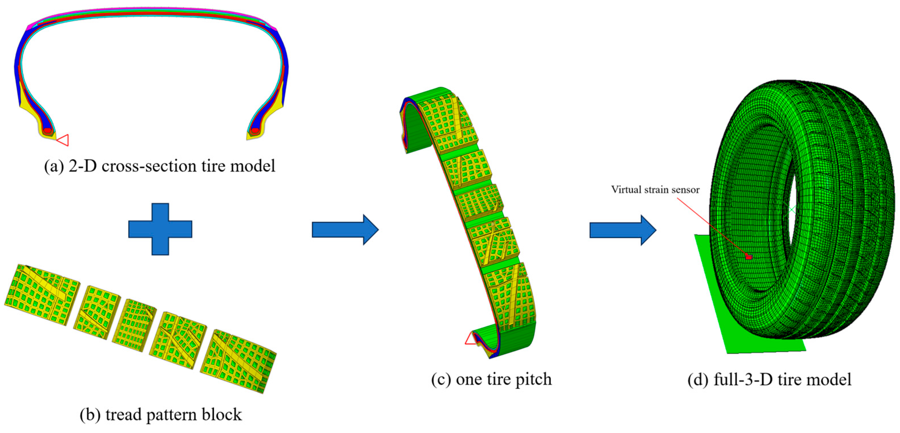
The tire model built in this article is a 205/55R16 radial tire, which is used as the object of simulation research; a tire is not made of a single rubber material but various materials. The structure is relatively complex. Therefore, a finite element model is established, which is divided into structural and tread pattern models. First, the 205/55R16 tire was cut in the laboratory to obtain the cross-sectional structure of the tire. A 2D axisymmetric structure model was established based on the reality tire structure profile and material distribution, in which the rubber element types are CGAX3H and CGAX4H, and the reinforcing materials, such as the carcass and belts, were established by the SFMGA1 plane element. The rubber solid element is embedded with rebar elements to simulate the features of the tire cord rubber composite material. The geometric parameters of the reference tread pattern blocks are used to import a 2D cross-section tire model into ABAQUS 2020 software. The 2D cross-section tire model is rotated to create a 3D solid mesh model with a single pitch using the *REVOLVE keyword.
Secondly, the single-pitch 3D tread pattern solid model is established using the CATIA 2017 software and imported into the HYPERMESH 2019 software to generate the 3D mesh, as shown in Figure 1b. Considering the incompressibility of rubber materials, the corresponding grid type is the hybrid element C3D8RH [17]. Fit the single structure tread pattern model using the tie command to form a sector tire model with 6°. Finally, the 3D tire model, including the complex tread pattern, is shown in Figure 1d, with 123,842 elements and 155,703 nodes, generated using the keyword *SYMMETRIC MODEL GENERATION.
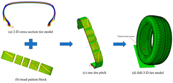
Figure 1.
205/55R16, the process of creating a finite element model for a tire.
The carcass layer, belt layer, and crown belt layer are all composed of cord rubber composites. In the finite element analysis model, the cord material (steel cord and nylon fabric) is defined as linear elastic material, and its mechanical property parameters can be obtained through the uniaxial tensile test. The cord material parameters of 205/55R16 radial tire obtained from the tensile test are shown in Table 1.

Table 1.
Parameters of the cords.
We specify the contact properties between the tire tread and road as hard contact and model the variation in the friction coefficient between the tire tread and road with slip speed using the Coulomb friction model.
The tire’s rubber material exhibits typical viscoelastic, incompressible, and doubly nonlinear characteristics of both material and geometry. The accuracy of the material model significantly impacts the analysis’s convergence during dynamic tire performances. Building upon our team’s prior research, the Yeoh model represents the rubber material [18], as defined in Equation (1):
where , , and are material constants; and is the first strain invariant:
where (i = 1, 2, 3) values are stretch ratios and the square root of the right Cauchy–Green strain tensor (C).
2.2. Experimental Verification
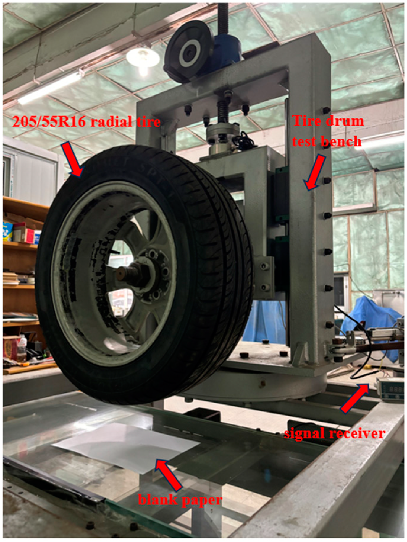
To verify the accuracy of the tire finite element model established, the results were verified using the tire static ground contact distribution characteristics test and tire radial stiffness test. The tire static ground contact test was performed using tire drum testing machine, as shown in Figure 2. During the test, the tire was loaded to a rated load of 3800 N, and the inflation pressure of 210 kPa was selected based on the tire manufacturer’s rated specifications for passenger vehicles under standard loading conditions. The additional 250 kPa case was included in our analysis. The wear of the test tire is 0, the environmental stability is 25 °C, and the pavement roughness is negligible. These conditions are consistent with the simulation conditions of steady rolling in the finite element simulation. The ground contact patch of the tire under static loading was obtained through red ink printing, and the ground contact geometric parameters were extracted, as shown in Figure 3. Table 2 shows that the error between the tire contact sizes obtained by finite element simulation and the test result are less than 2%, which has a high accuracy, indicating that the tire finite element model established in this paper can accurately describe the tire ground contact characteristics.

Figure 2.
Tire stiffness test bench.
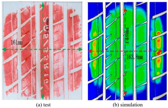
Figure 3.
Comparison of the sizes of the contact patch tire.
Table 2.
Tire ground contact characteristics.
To further verify the accuracy of the tire finite element model, a comprehensive strength testing machine was used to conduct tire radial stiffness test. The test and simulation results of tire sinkage and static loading radius under different test conditions are shown in Table 3, and the test and simulation results of radial stiffness are shown in Figure 4. It can be seen from the table and figure that the tire sinkage, static loading radius, and radial stiffness of the test and simulation show good consistency.
Table 3.
Comparison of test and simulation results of tire sinkage and static loading radius.
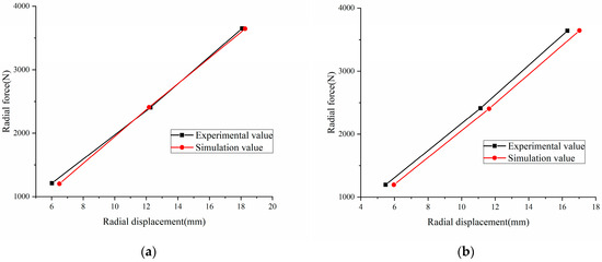
Figure 4.
Comparison of tire radial stiffness under different inflation pressures: (a) 210 kPa and (b) 250 kPa.
2.3. Extraction of Circumferential Strain Signals
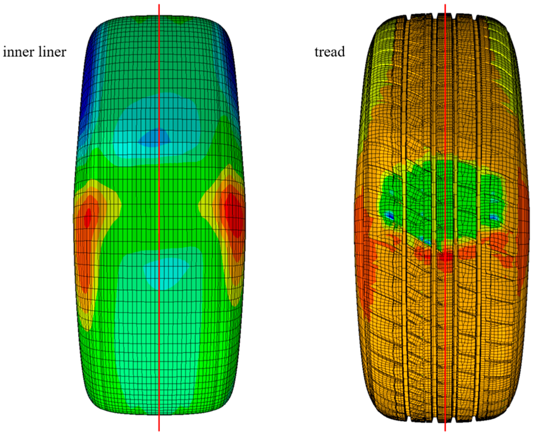
The selection of intelligent tire sensors mainly includes three-axis accelerometers, strain sensors, optical sensors, and others [19]. Strain sensors offer advantages such as high precision, wide measurement range, fast response, durability, reliability, and ease of installation and integration. Compared to accelerometers, the signals from strain sensors are less susceptible to interference from tire noise. Based on the previous research conducted by the research team on the force-sensitive response regions of tires, it was found that, under braking conditions, the deformation caused by the contact between the tire and the ground primarily occurs at the tread. Therefore, in steady-state rolling simulation analysis, with the highest point of the rolling tire as 0 point, the circumferential strain signals of the centerline of the tread and the centerline of the inner liner are extracted, respectively, by rotating for one cycle. Comparative analysis of circumferential strain signal characteristics of tread centerline and liner centerline is as shown in Figure 5. The abscissa represents the distance of the nodes around the tire during one revolution, while the ordinate represents the circumferential strain signal. According to Figure 6, it can be found that the tread pattern significantly influences the circumferential strain signal at the tread centerline, resulting in large fluctuations in the signal, which are particularly evident at the signal’s troughs. This fluctuation hinders the effective extraction of sensitive signal features.
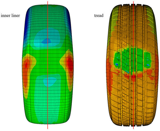
Figure 5.
Strain signal extraction locations.
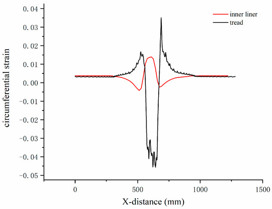
Figure 6.
Comparison of circumferential strain signals between tread and inner liner.
Compared to the circumferential strain signal at the tread centerline, the strain signal at the inner liner centerline is less affected by the tread pattern. The signal curve is smoother and more stable, with its trend opposing the tread centerline strain signal. This discrepancy is primarily related to the tire’s structure, material properties, and load transmission. When the tire is subjected to external loads and in contact with the ground, the tread experiences compression and elongation due to frictional forces, resulting in significant localized deformation. The tire structure is multi-layered and composite, and due to the differing elastic moduli and response characteristics between the tread and the inner liner, the inner liner undergoes deformation that is opposite to that of the tread. Therefore, by extracting the circumferential strain signal of the point in the inner liner centerline under the rolling tire braking condition, the signal is selected to represent the real-time strain sensor signal of the rolling tire [20]. The specific location of this point is shown in Figure 1d.
3. Estimate Contact Patch Length
3.1. Estimating Contact Angles
Using the circumferential strain signal at a point on the longitudinal centerline of the inner liner of a rolling tire as a research object, contact pressure signals were extracted in Abaqus for one week of rolling tire tread midline. A characteristic analysis of circumferential strain signal and contact pressure signal was performed. To obtain circumferential strain signals during braking of 205/55R16 radial tire, set the tire load condition as 3800 N, inflation pressure as 210 kPa, and road friction coefficient as 0.5. Then, adjust the rolling angular velocity of the tire to control the slip rate to 0.08 at a linear speed of 70 km/h. The strain signal curves were interpolated and smoothed to compare the signal characteristics better.
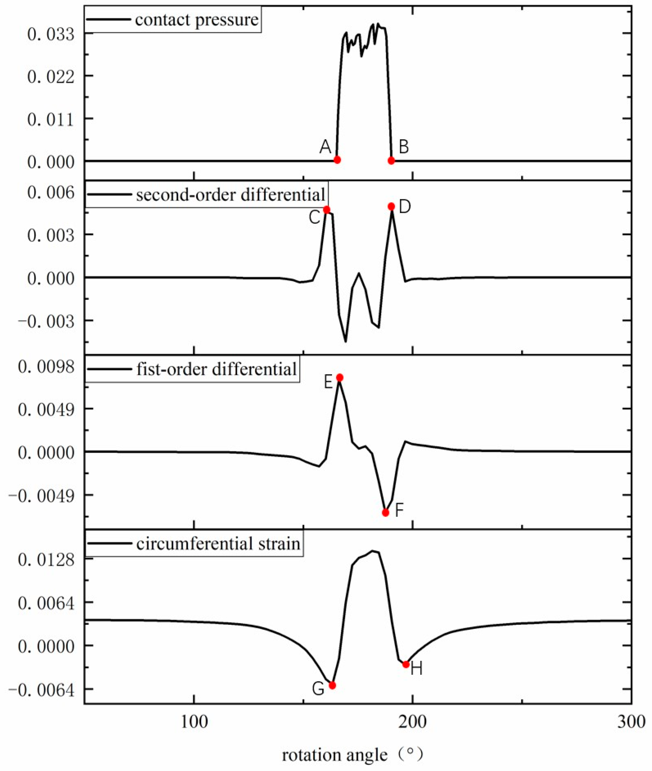
Figure 7 shows the first and second order derivatives of the circumferential strain signal compared to the contact pressure signal. The actual contact angle, , of a rolling tire can be obtained from the boundary conditions of the contact pressure signal. The characteristic angles, , of the circumferential strain signal curve were extracted separately. Then, we extracted the characteristic angle, , of first-order derivative strain signal curve; and the characteristic angle, , of the second-order derivative strain signal curve. The difference between the tire’s actual contact angle and the characteristic angle of the first-order and second-order derivative curves of the circumferential strain is approximately 3°. The characteristic angle of the circumferential strain signal differs from the tire’s actual contact angle by about 10°, as shown in Equation (3).
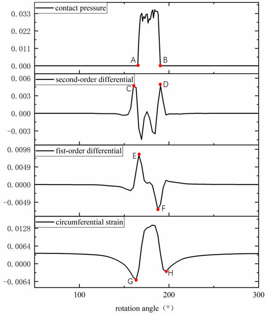
Figure 7.
Comparison between peak angle difference of circumferential strain of tire inner liner and contact angle.
This trend is consistent with the experimental results in Reference [21]; the characteristic angle of the circumferential strain’s first and second derivative curves is selected as the characterization index of the contact angle, as shown in Equation (4).
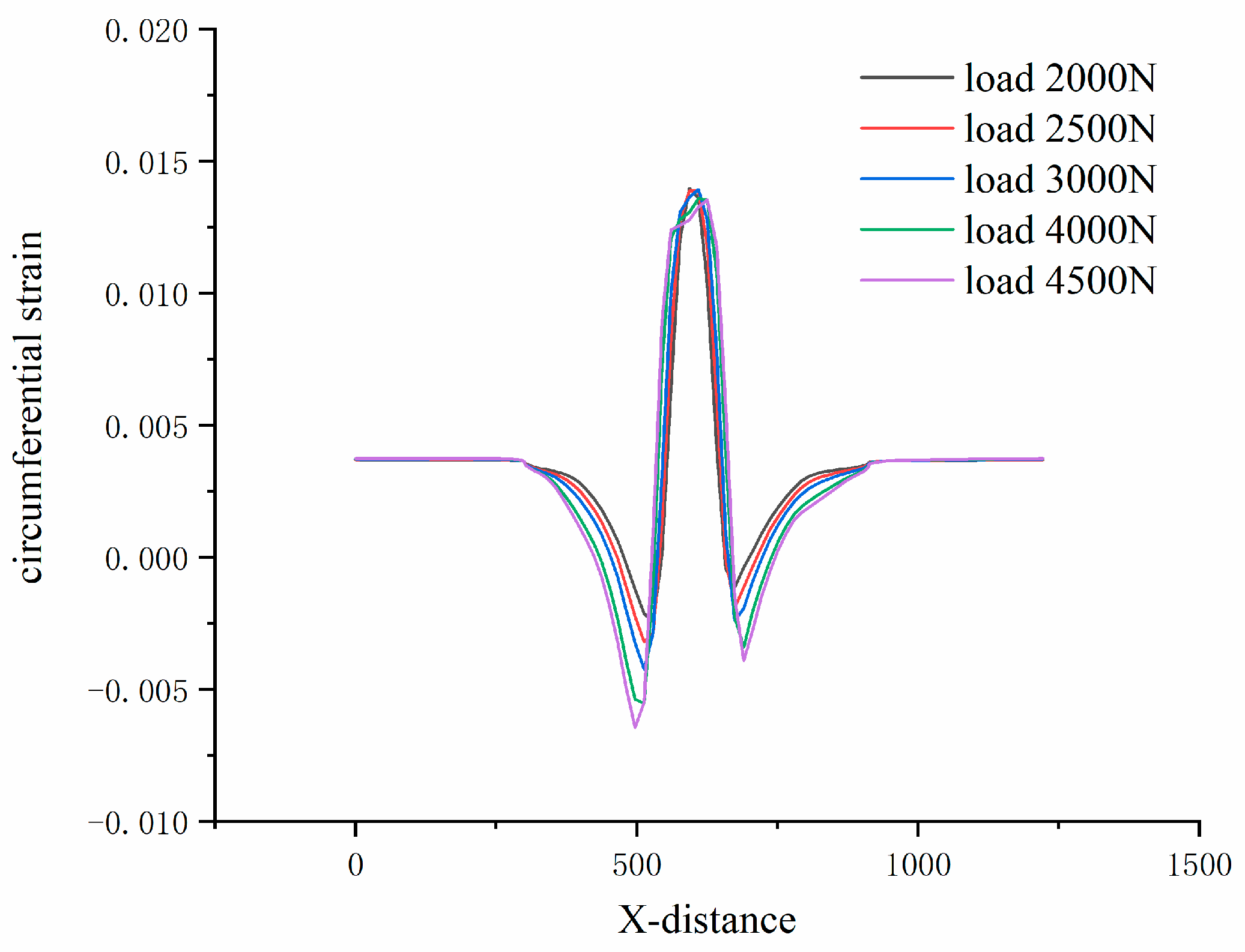
To further analyze the characteristic angles of rolling tire circumferential strain signals, with other tire parameters unchanged, simulation analyses were carried out using finite elements for load conditions of 2000 N, 2500 N, 4000 N, and 4500 N, respectively. Circumferential strain signals were acquired at the midline of the inner liner within the tire contact patch, and the contact angle was simulated, as shown in Figure 8. It was found that the two troughs of the circumferential strain signal increased with increasing loads, and the angular difference between the two troughs increased; this is due to the increased load, increased deformation of rolling tire treads, and the contact angle between the tire and the ground increases. The absolute values of the signals on both sides of the peak also increase with increasing load. However, the circumferential strain signal at the center of the rolling tire–road contact zone decreases with increasing load because the tire has “buckled” [22,23]. The fluctuation of the peak signal is due to the presence of the tire tread pattern; since the extracted signal characteristic value is the angular difference between two troughs, the signal fluctuations of the peaks do not affect the estimation of the rolling tire contact angle.
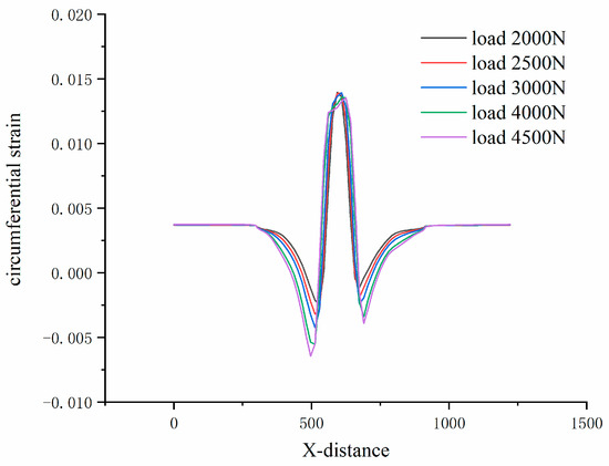
Figure 8.
Circumferential strain signals under different loads.
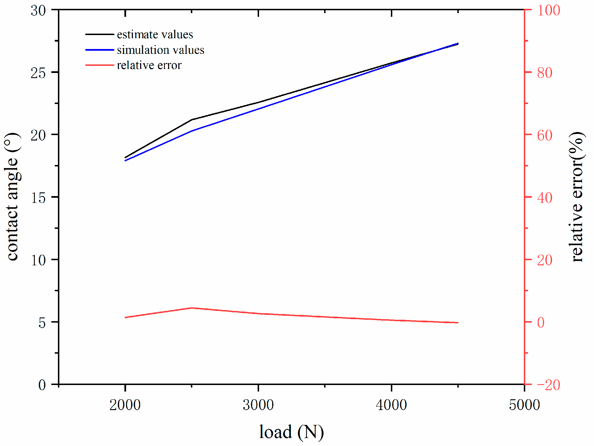
Equation (2) was used to estimate the contact angle between a rolling tire and the ground, compare the estimated and simulation values of the contact angle, and describe the estimation accuracy of this method in terms of relative error. The results are shown in Figure 9. The maximum difference between the estimated and simulated contact angle is about 1°, and the maximum relative error of estimation is not to exceed 5%; it was verified that the contact angle estimation method is feasible.

Figure 9.
Estimated and simulated values of contact angle under different loads.
3.2. Estimating Contact Patch Length
The content in the previous section determines the estimation method of the contact angle of rolling tires; the finite element analysis method was used to simulate the rolling tires with slip rates of 0, 0.02, 0.04, 0.06, 0.08, and 0.1; the load is 3800 N; the inflation pressure is 210 kPa; and the road friction coefficient is 0.5.
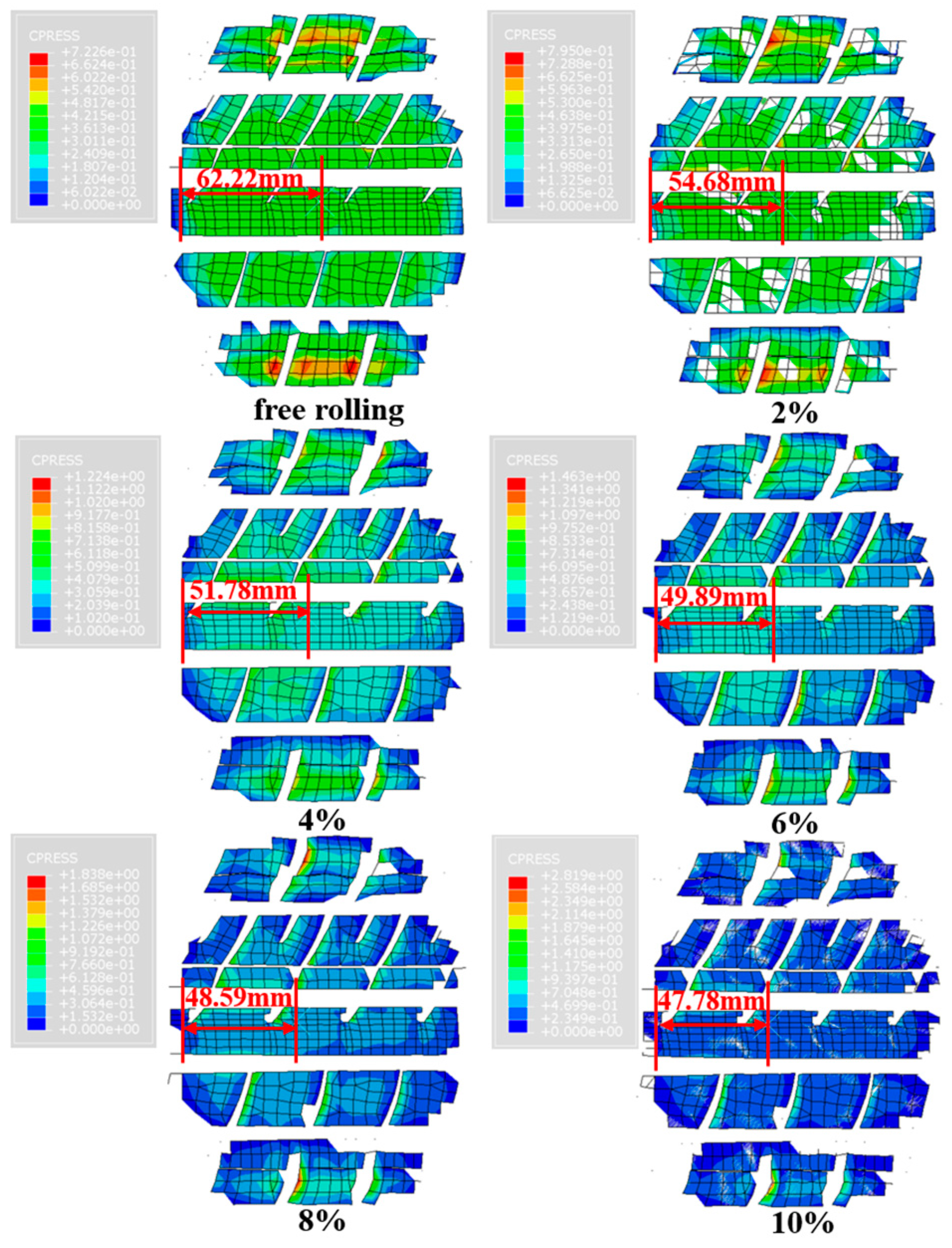
Figure 10 shows the contact patch of the rolling tire under different slip rates. It can be seen that the front and rear contact angles are equal when free-rolling. When the tire begins to slip, the position of the midpoint of the tread in the finite element simulation starts to move forward, and the front contact angle decreases with the increase in slip rate; and the rear contact angle increases with the increase in slip ratio, an increase in asymmetry of contact angle. When the tire is at a high slip rate, the increasing trend of asymmetry of contact angle becomes slow; this is consistent with the results of Reference [24]. Therefore, the assumption that the front and rear contact angles of tires are equal cannot be used to estimate the contact patch length during braking. Using the arc length formula relative to the trigonometric function does not allow us to distinguish the size of the front and rear contact angles; it is more suitable for estimating the contact patch length of rolling tire during braking. The estimation formula of contact patch length is shown in Equation (5).
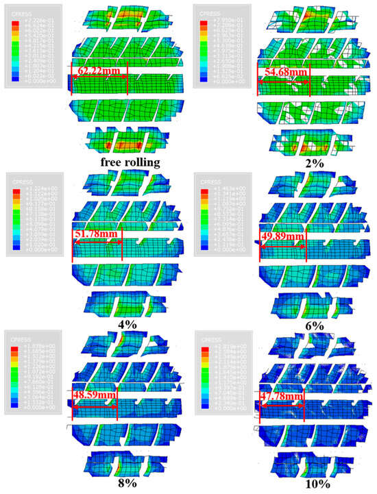
Figure 10.
Comparison of asymmetric contact angles.
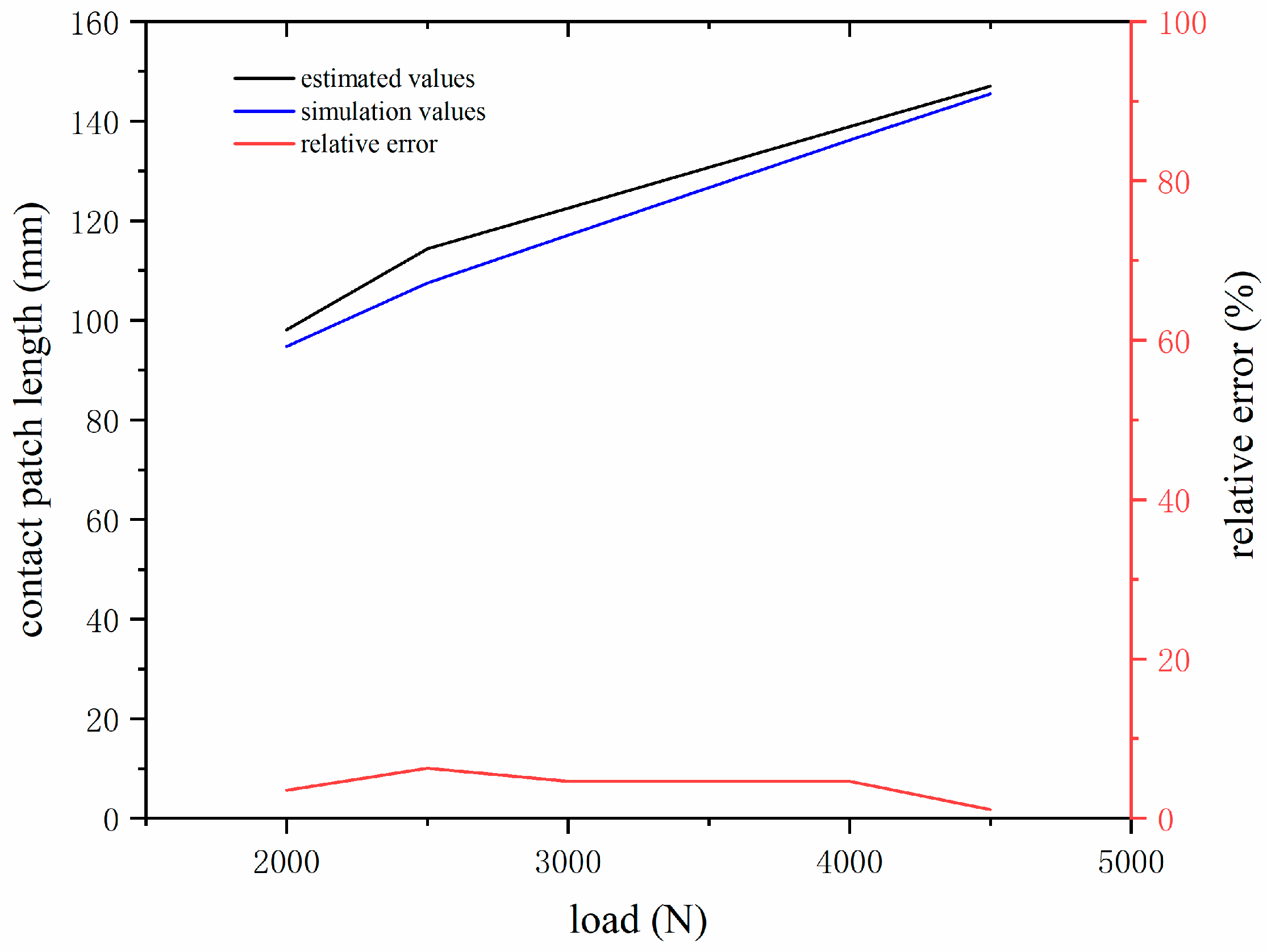
Figure 11 shows the estimated contact patch length of the rolling tire under different loads, compared with the simulation value of contact patch length obtained by finite element simulation. It can be seen that the length of the arc is greater than the length of the straight line, the estimated contact patch length is larger than the simulation result, and the relative error exceeds 6%. When rolling tires under low and high load conditions, the error between the estimated value and the simulated value is small, and it is greater at moderate loads. In order to reduce the error of the estimated contact patch length, we define a correction factor β to eliminate the length difference between the arc length and the straight line, as shown in Equation (6).
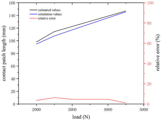
Figure 11.
Estimation and simulation values of contact patch length under different loads.
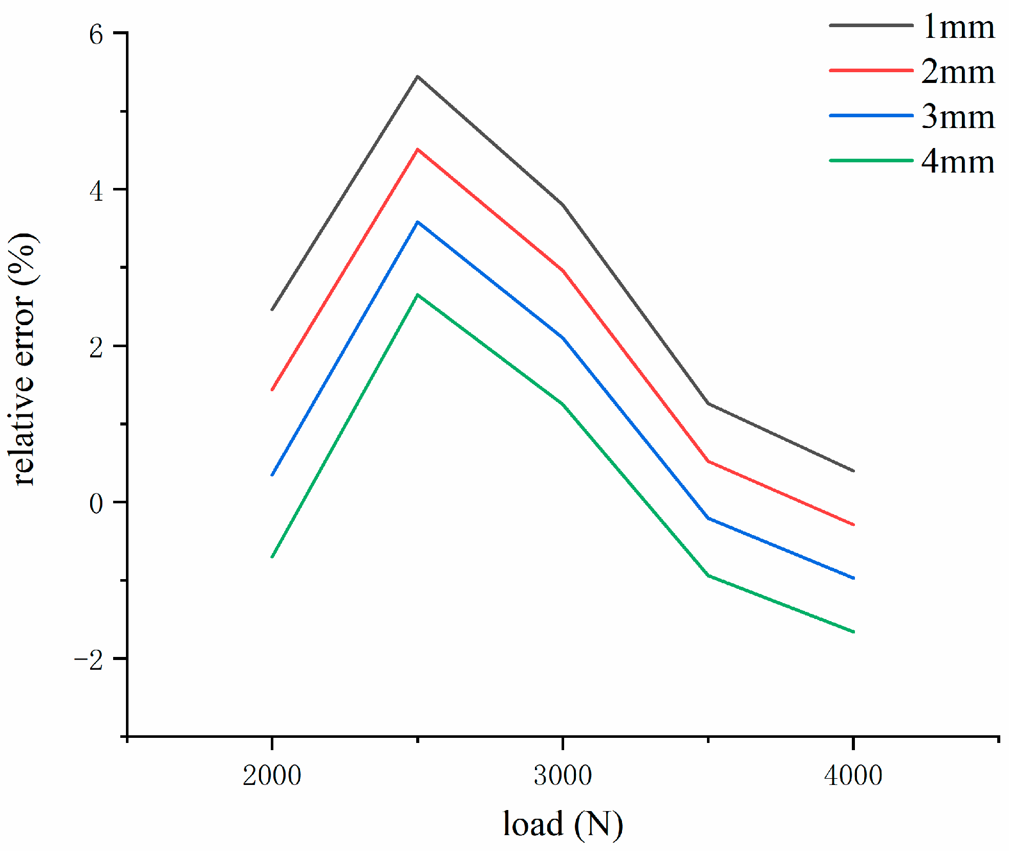
To determine the value of the correction factor, β, values of β were chosen as 1 mm, 2 mm, 3 mm, and 4 mm to calculate the relative error in the contact patch length for each correction factor, as shown in Figure 12. It can be observed that as the value of β increases, the estimation accuracy of the contact patch length improves. However, at higher and lower loads, the relative error of contact patch length estimation first decreases and then increases. When the tire is under extreme conditions of low and high load, the safety requirements of the vehicle are higher, so the active safety control system of the vehicle needs more accurate input. The contrast correction factors are 1 mm, 2 mm, 3 mm, and 4 mm; the average relative error under lower and higher loads was found to be 0.63% at 3 mm; and 0.63% at 1 mm, 2 mm, and 4 mm were 1.43%, 0.865%, 1.18%, respectively. After considering the overall performance for different values of β, a correction factor, β, of 3 mm was selected.
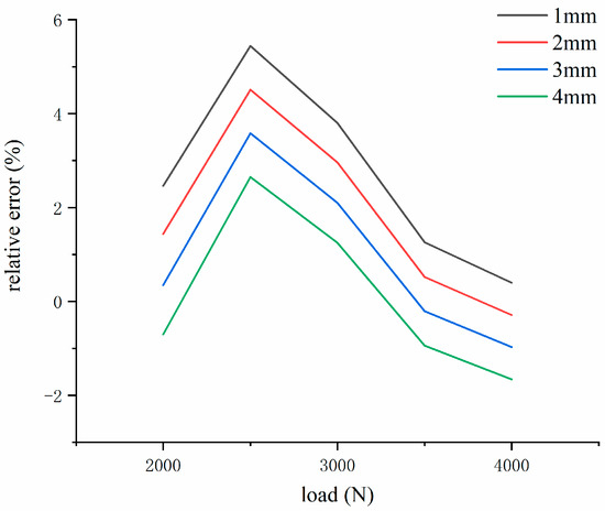
Figure 12.
Relative error of different correction factor values.
3.3. Estimating Contact Patch Length Under Different Working Conditions
In the previous section, the contact angle and contact patch length of a rolling tire under different loads during braking were established and verified. To further validate the generalizability of this method, relative errors were analyzed by comparing the contact angle and contact patch length estimates with the simulated values, changing the operating conditions and physical parameters of the rolling tire during braking.
3.3.1. Road Condition
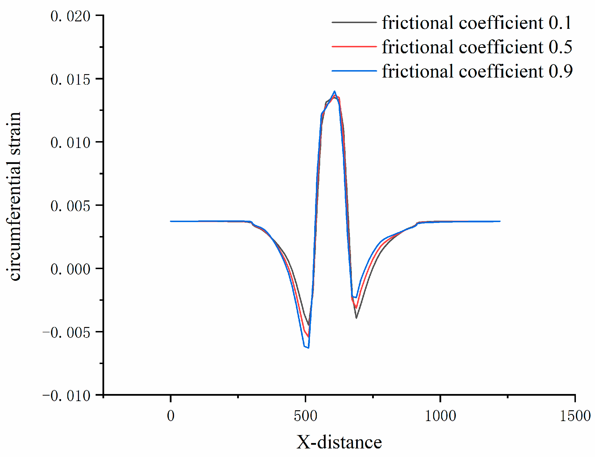
In the finite element modeling of tire ground contact, a two-dimensional plane is defined as an analytical rigid body, and then it is loaded to make it contact with the tire. Considering the complexity of road conditions, this study mainly represents different road conditions by comparing the road with different friction coefficient. Only the friction coefficient is different, and other road condition parameters remain the same in the simulation. Three different friction coefficients of 0.1, 0.5, and 0.9 were set in Abaqus by finite element simulation software to simulate the braking process of rolling tires under three different road conditions. The estimation was completed using the established estimation method of contact angle and contact patch length. The tire load is 3800 N, the inflation pressure is 210 kPa, and the rolling tire slip rate is 8%. Figure 13 shows the circumferential strain signal of the rolling tire under different road conditions. It can be seen that with the increase in road friction coefficient, the peak value of circumferential strain signal in the center of contact patch of rolling tire increases, and the angle difference between the two troughs remains almost unchanged; this shows that the contact patch length of rolling tire is less affected by the road friction coefficient, and the absolute value of the trough also increases with the increase in the road friction coefficient [25].
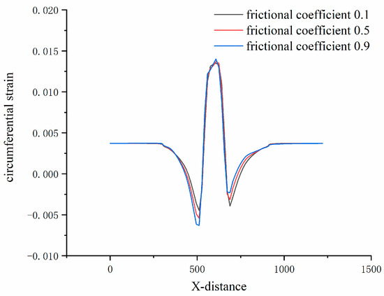
Figure 13.
Circumferential strain signals under different road friction coefficients.
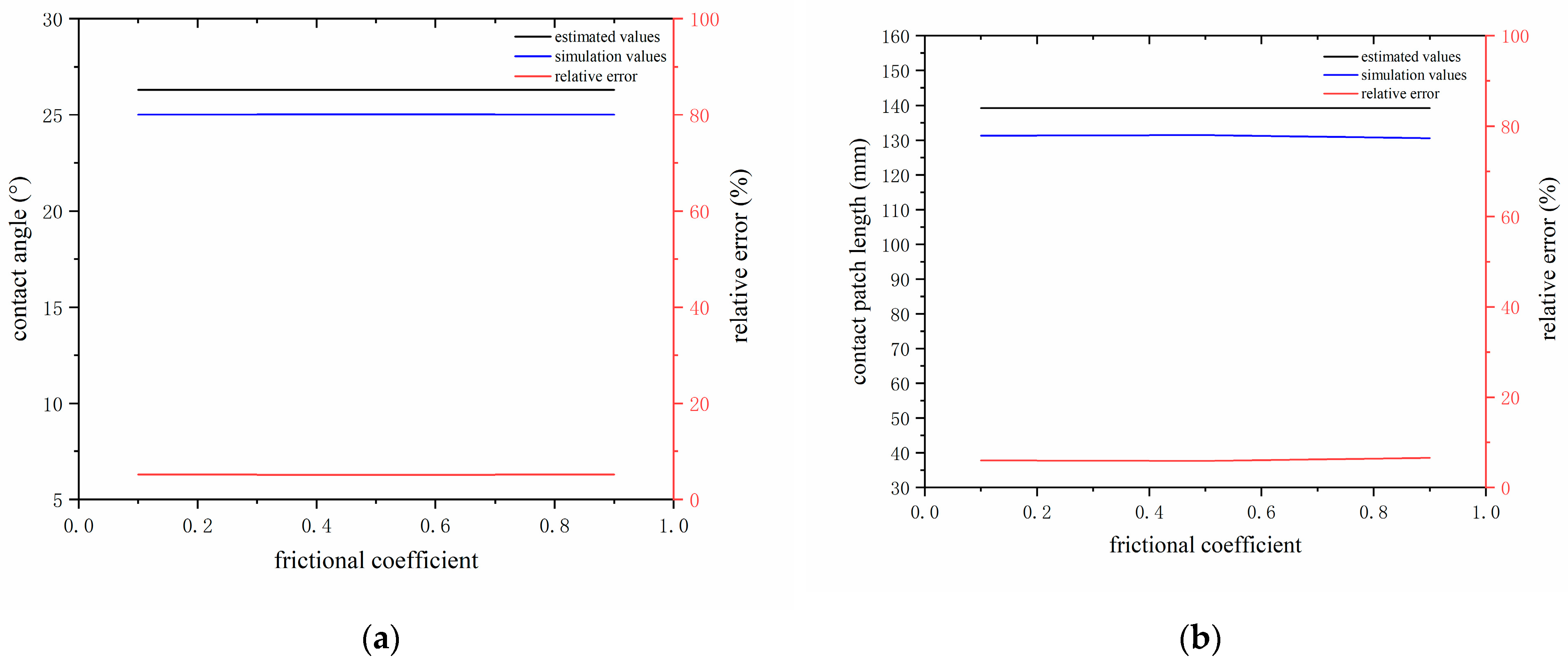
Figure 14 shows the estimated contact angle and contact patch length based on the extracted circumferential strain signal of the centerline of the inner liner. The change in road friction coefficient has little effect on the angle difference between the two troughs of the first- and second-order circumferential strain derivative curves. Therefore, it can be assumed that the estimated contact angles under different road friction coefficients are equal. However, in the finite element simulation software, due to the mesh of the tire model, there are some errors in extracting different road contact angles and contact patch lengths because of changes in road friction coefficients; even if the load does not change, it will also affect the contact pressure distribution in the tire contact patch. However, there are errors in the simulation values of the contact angle and the contact patch length of the rolling tire, but they are consistent. Therefore, it can be proved that when the rolling tire is braked, other operating parameters are consistent, changing pavement conditions only, which will not affect the tire contact angle and contact patch length. The maximum error of tire contact angle estimation is 5.16%, within 2°, and the maximum error of contact patch length estimation is 6.58%, not exceeding 10 mm.
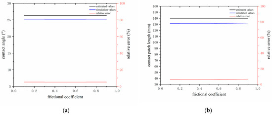
Figure 14.
Estimated and simulated values of grounding parameters under different road friction coefficients: (a) contact angle and (b) contact patch length.
3.3.2. Slip Rate
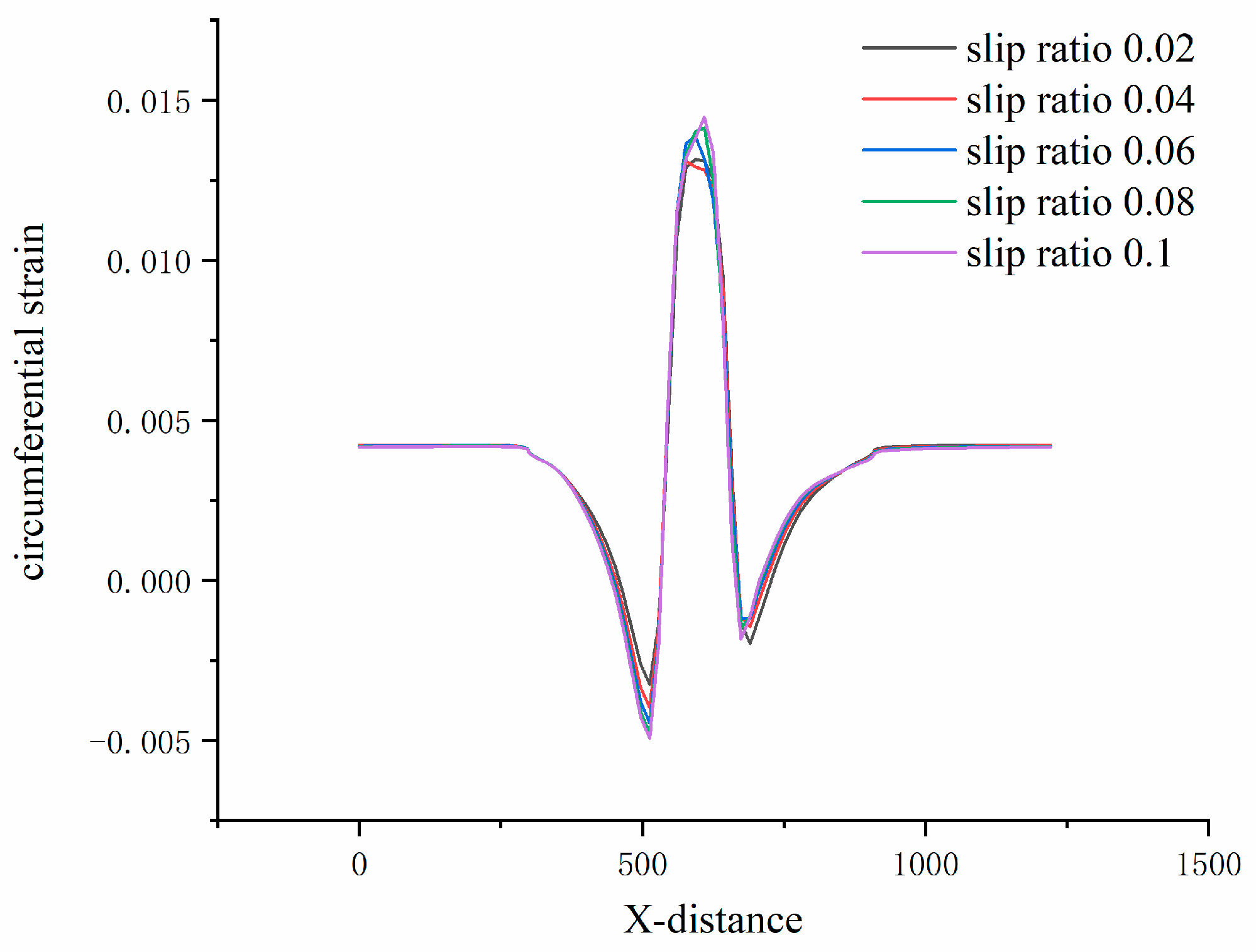
The circumferential strain signals of the tread centerline of rolling tires at slip rates of 0, 0.02, 0.04, 0.06, 0.08, and 0.1 were extracted by finite element simulation, as shown in Figure 15. The load is 3800 N, the inflation pressure is 210 kPa, and the road friction coefficient is 0.5. With the increase in slip rate, the absolute value of the strain signal trough at the front end of the contact patch increases; it moves forward slightly, and the absolute magnitude of the trough of the strain signal at the back end is unchanged [26]. It can be concluded that rolling tires during braking and other conditions remain unchanged, and the change in slip rate has little effect on tire contact angle. However, the asymmetry between the left and right sides will increase with the increase in tire slip rate. The valley value of the circumferential strain signal peak increases with the slip rate increase; however, when the tire reaches 6% slip condition, the valley value changes slightly, which mainly affects the distribution of the strain signal.
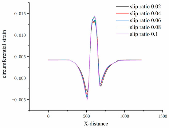
Figure 15.
Circumferential strain signals at different slip rates.
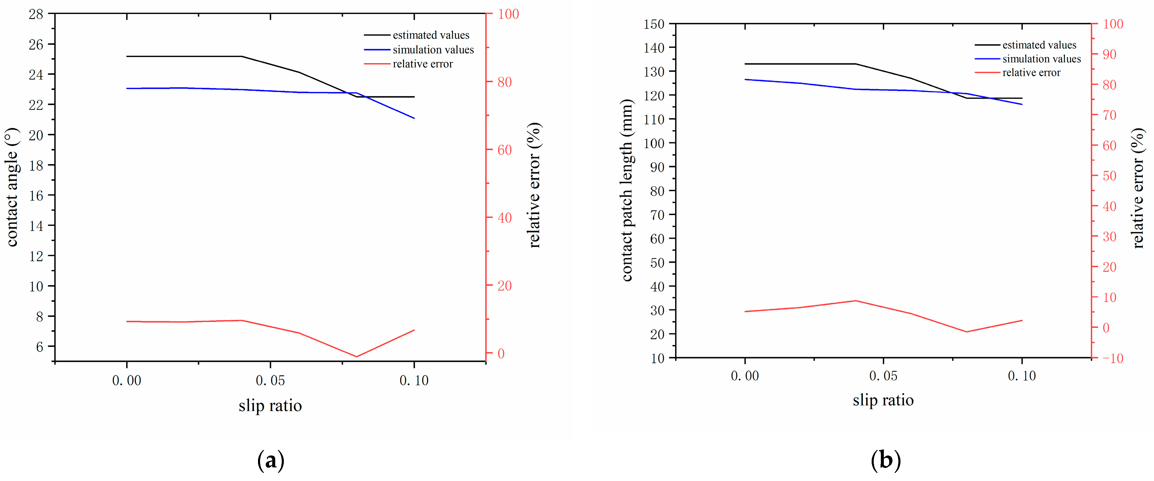
Figure 16 shows the estimated and simulated contact angle and contact patch length values under different slip rates and relative errors. The estimated value of the contact angle is generally significant. However, the maximum relative error is less than 10%, the maximum difference between the estimated contact angle and the simulated value is about 2°, the maximum relative error between the estimated and simulated contact patch length is 8.68%, the minimum error is 1.14%, and the average error is not more than 5%.
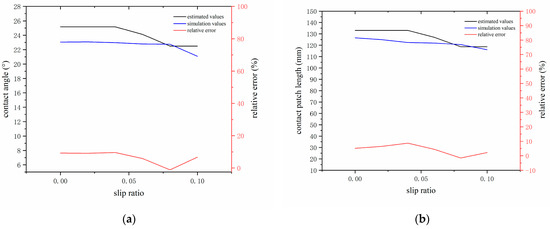
Figure 16.
Estimated and simulated values of grounding parameters under different slip ratios: (a) contact angle and (b) contact patch length.
3.3.3. Inflation Pressure
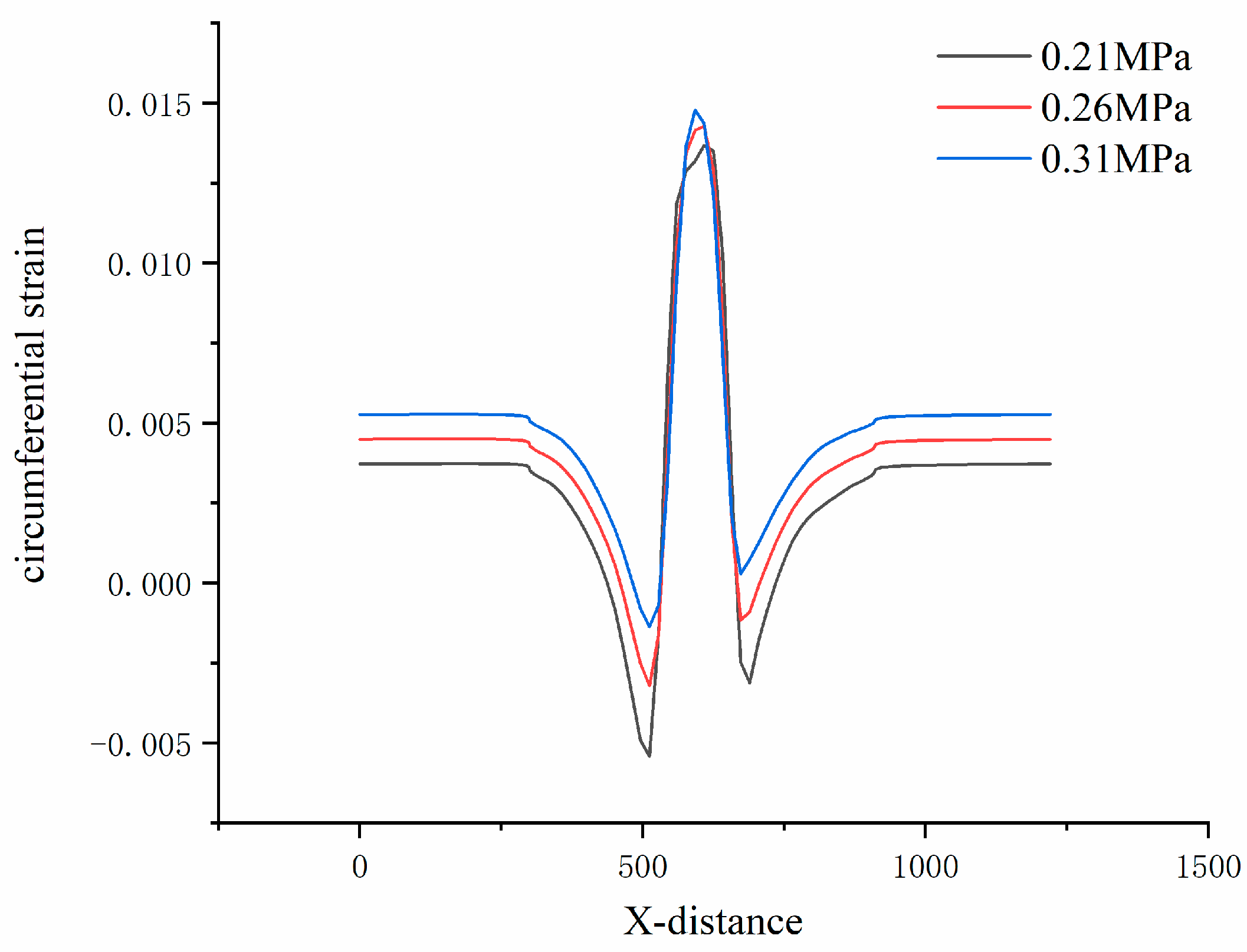
Through finite element simulation, the circumferential strain signals of the rolling tire under the conditions of inflation pressure of 210, 260, and 310 kPa during braking were extracted. The load is 3800 N, the road friction coefficient is 0.5, the slip rate is 8%, and the tire wear is 0 mm, as shown in Figure 17. It can be seen that the absolute value of the trough at the front of the contact patch of the rolling tire decreases with the increase in inflation pressure, and the peak value of the back end wave decreases with the increase in inflation pressure. The difference between the two troughs is also affected by inflation pressure, and the peak value of circumferential strain signal increases with the increase in inflation pressure [27].
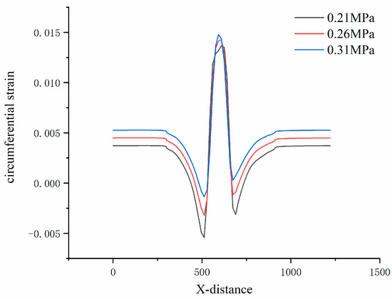
Figure 17.
Circumferential strain signals under different inflation pressures.
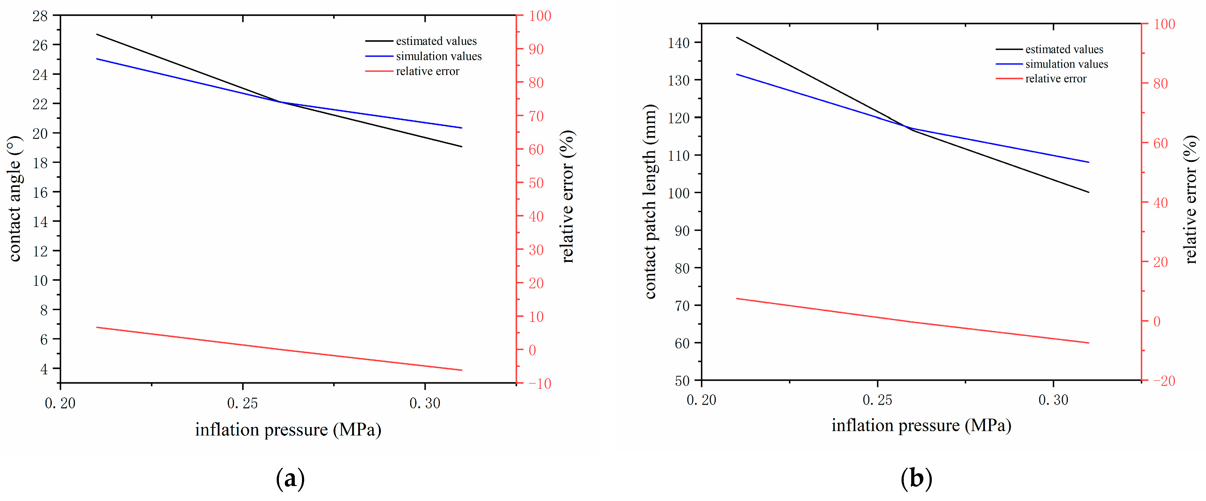
Figure 18 shows the estimated and simulated values and relative errors of contact angle and contact patch length under different inflation pressures. It can be seen that the relative error of the estimated contact angle is the smallest when the inflation pressure is 210 kPa; the relative error is significant under slight inflation pressure and considerable inflation pressure, but not more than 8%. At the same time, the relative error of contact patch length is the smallest at medium inflation pressure, the relative error is significant under small and large inflation pressure, and the maximum error is about 8 mm.
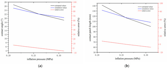
Figure 18.
Estimated and simulated values of grounding parameters under different inflation pressure: (a) contact angle and (b) contact patch length.
4. Estimated Vertical Force
4.1. Feature Extraction of Circumferential Strain Signal
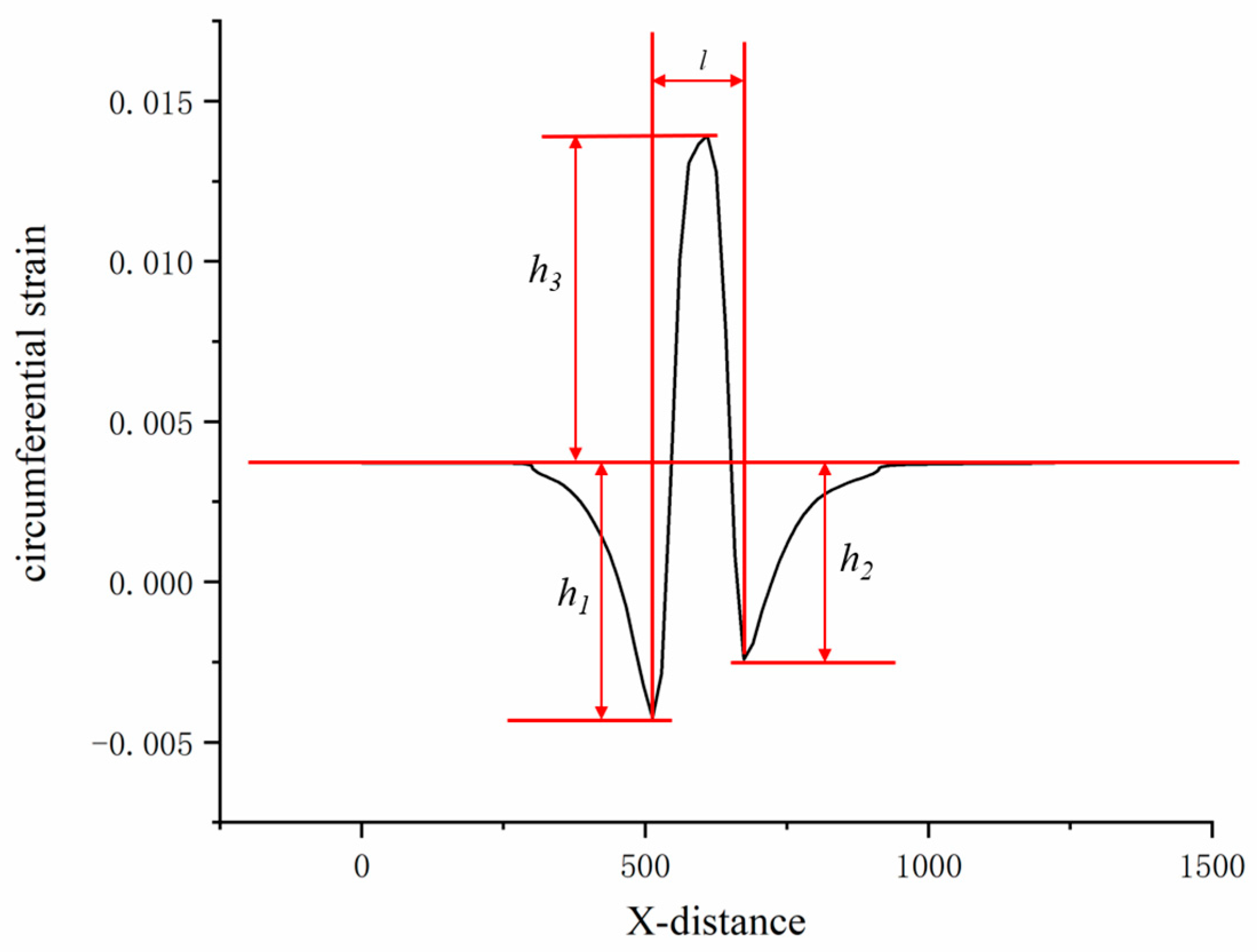
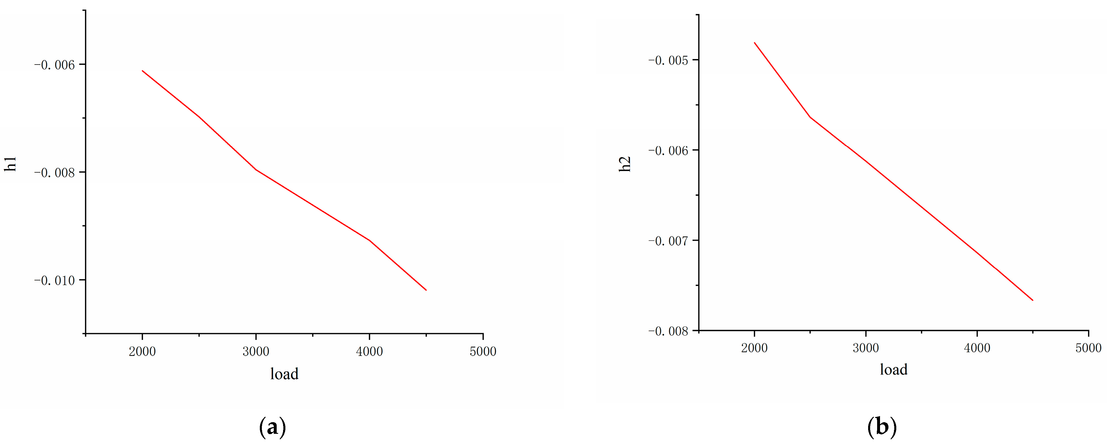
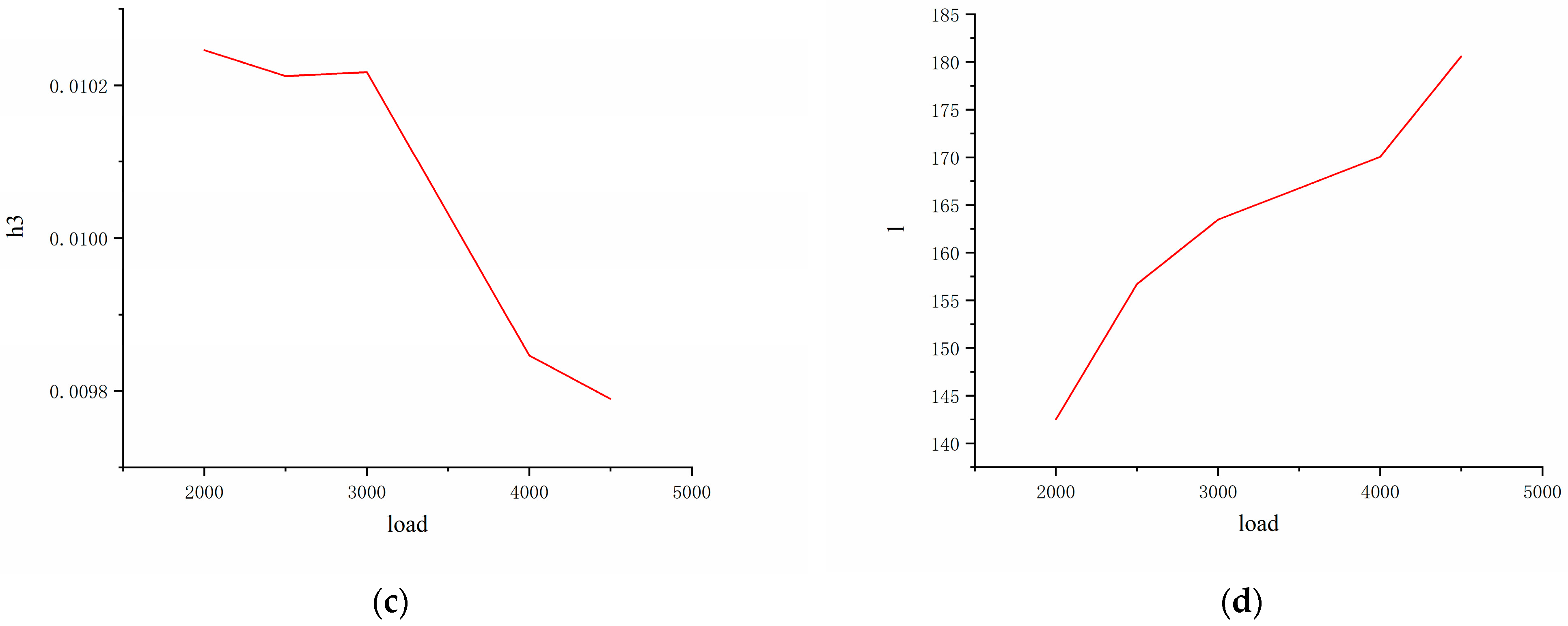
According to the analysis results of sensitive response signals under different loads, select the circumferential strain signal of the centerline of the inner liner of the rolling tire for feature extraction, as shown in Figure 19. The two troughs, h1 and h2, of the circumferential strain signal; the distance, l, between the two troughs; and the peak of the wave, h3, were selected. Feature extraction and analysis of circumferential strain signals in the medial line of tire inner liner under different loads with inflation pressure 210 kPa, slip rate of 0.08, and tread wear of 0 mm were performed by combining finite element simulation. We plotted the relationship between characteristic values and loads as shown in Figure 20.
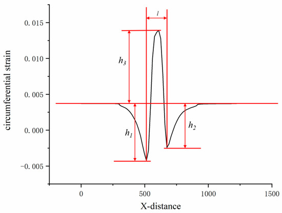
Figure 19.
Feature extraction of circumferential strain signal.
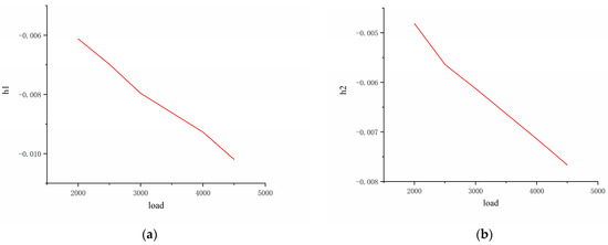
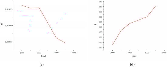
Figure 20.
Relationship between characteristic values of strain signal and vertical force.
Figure 20 shows the following: (1) During the load increase from 2 kN to 4.5 kN, the contact compression deformation between tire and ground increases, and the area of contact area becomes larger. The tensile deformation increases in the noncontact area, reducing the regional deformation outside the noncontiguous area. (2) The peak value, h3, of the circumferential strain signal’s response curve at the inner liner’s center line has an overall increasing trend. However, there is a significant increase when the vertical load is 3 kN, making h3 tend to become irregularly large. This is due to the presence of the tread pattern, which causes the center of the tread to be squeezed by the tread blocks, and the peak pressure in the contact area is thus compromised. (3) The absolute value of h1 in the circumferential strain signal trough of the inner liner centerline decreases approximately linearly with the change in vertical load. The absolute value of the circumferential strain signal trough, h2, in the inner liner also shows an overall approximately linear decreasing trend. Unlike h3, the characteristic values h1 and h2 do not affect the circumferential strain signal due to the transverse grooves of the tire tread; irregularities were observed near the vertical load of 3 kN. (4) The trough spacing, l, increases from 142.513 mm when the vertical load is 2 kN to 180.599 mm when the vertical load is 4.5 kN, showing an approximate linear growth trend of “rapid growth—slow growth—rapid growth”. Considering the influence of the tire tread pattern on the characteristic value, h3, the vertical force estimation model developed in this paper can be adapted to different tire types and complex driving conditions. This paper chooses h1, h2, and l, which have a more precise linear relationship with the vertical force, as the sensitive response eigenvalues of the vertical force training model. To have enough training samples and improve the prediction model’s estimation accuracy, extend the variation in vertical loads from 500 N to 5 kN in simulations. The data set working condition settings are shown in Table 4.
Table 4.
Data set condition setting.
4.2. BP Neural Network Optimized by Particle Swarm Optimization
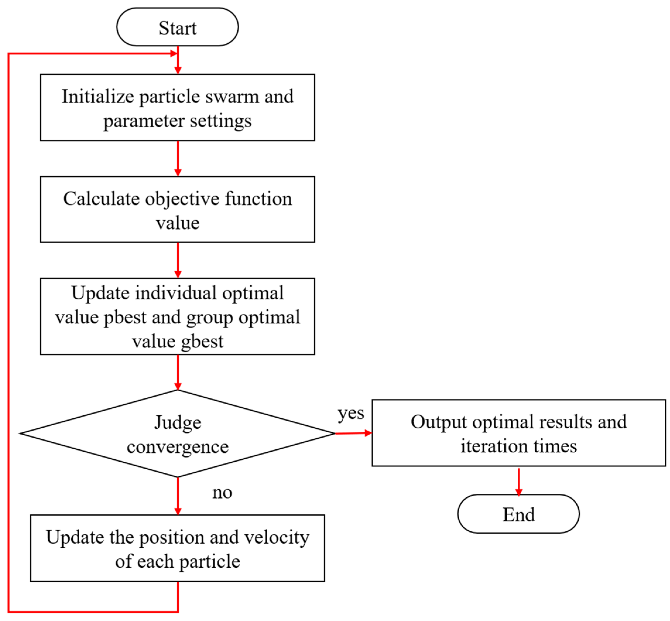
Particle swarm optimization (PSO) is a global optimization algorithm that was proposed by Kennedy and Eberhart in 1995 to simulate the foraging behavior of birds in nature [28]. The basic idea of particle swarm optimization is to find the optimal solution in the search space through each member of the bird swarm; each particle group can exchange information, and the position and velocity of each particle represent a possible solution in the problem solution space. The user updates speed and position during the search based on two extremes: the first is the optimal solution found by the particle itself—this solution is called the individual extreme value best; the other extreme is the optimal solution found so far by the whole population. The computational flow of the particle swarm algorithm is shown in Figure 21.

Figure 21.
Particle swarm algorithm computational flow diagram.
The velocity and position of each particle is defined as follows:
where is the velocity of the particle; is the position of the particle; and are the learning factors, which generally take the value of 2; and are random numbers between (0, 1); N is the total number of particles in the swarm; and is the weight. The first term in Equation (7) is a memory term indicating the effect of the last velocity and direction. The second term is the self-cognition term, which is a vector pointing from the current point to the particle’s own best point, indicating the part of the particle’s action that originates from its own experience. The third term of the formula is a vector pointing from the current point to the best point of the population, reflecting the synergy and knowledge sharing between particles. The article is the one that decides the next movement through its own experience and the best among its peers.
BP neural networks are characterized by both multi-layer feed-forward networks and error backpropagation. They mainly consist of input, hidden, and output layers and can handle nonlinear problems through layer-by-layer transfer and error backpropagation [29]. The training of a BP neural network is divided into two main processes: the forward propagation of data from the input layer through the hidden layer and, finally, to the output layer; and the second is the backpropagation of errors. First, the error between the actual output and the target output is calculated at the output layer; then, from the output layer to the hidden layer and finally to the input layer, the sizes of the weights and thresholds are continuously adjusted for each layer. Learning stops when the training error reaches the training set accuracy or the set number of training sessions; each time, it is computed via the chain rule and uses gradient descent to adjust the weights and bias according to the error gradient.
where is the error gradient, is the loss function, is the network weights, and is the output of the neuron.
where is the learning rate.
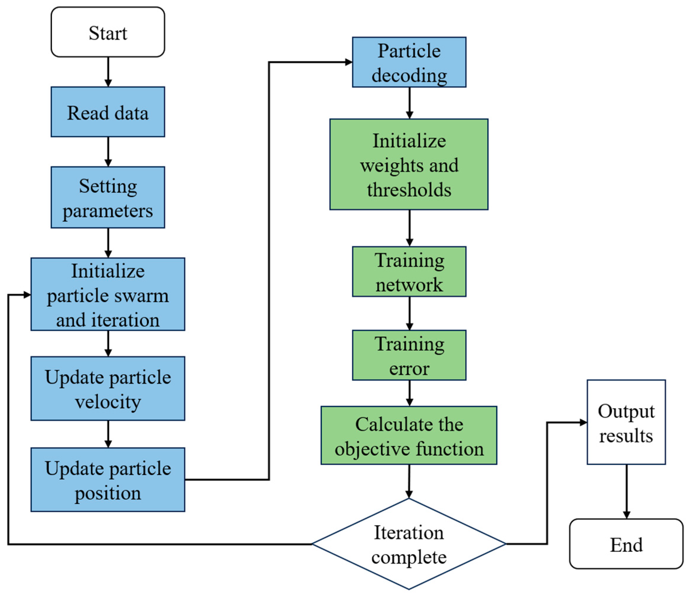
BP neural networks have easy applicability to nonlinear modeling, advantages of better fitting ability for complex input–output relationships, and the ability to improve the fitting ability and accuracy through multi-layer networks [30]. However, it also tends to fall into local optimal solutions, is computationally intensive, takes a long time to train, and is sensitive to the initial weights, which disadvantages the need to find a suitable initialization method. Therefore, in this paper, by combining the particle swarm algorithm and BP neural network, the weights and biases of the neural network can be optimized effectively; this solves the problem that the gradient descent method in traditional BP neural networks may fall into local optima. PSO-BP optimization algorithm uses particle swarm optimization algorithm to find the optimal neural network parameters, and these parameters are used to replace the weight adjustment steps in the traditional gradient descent method training process. The algorithm calculation process is shown in Figure 22.
Figure 22.
PSO-BP calculation flow diagram.
4.3. Training of Vertical Force Estimation Model
During the training of the prediction model, five groups of simulation schemes of the data set, a total of 120 groups of data, are divided into training sets; the last group of simulation schemes, a total of 24 data groups, is the test set [31]. Normalize the input training set and scale the data to 0–1; this is conducive to speeding up the particle swarm optimization BP neural network and improving the stability of the prediction model. According to the input data, including slip rate, inflation pressure, road conditions, h1, h2, and l, the input layer of the network is determined to be 6, output data are loaded, and we set the output layer to 1, and in order to ensure the prediction accuracy of the prediction model, the error threshold is determined to be 1 × 10−40, and the maximum number of iterations is set to 100. The magnitude of the learning rate also affects the training results of the predictive model: if the learning rate is too large or too small, there will be neural network oscillation, and the convergence speed of the phenomenon will be reduced. We usually take the value of the size of the interval of 0.01 to 0.2, so this paper selects the size of 0.01. The initial parameters of PSO-BP neural network are shown in Table 5.
Table 5.
PSO-BP neural network initialization parameters.
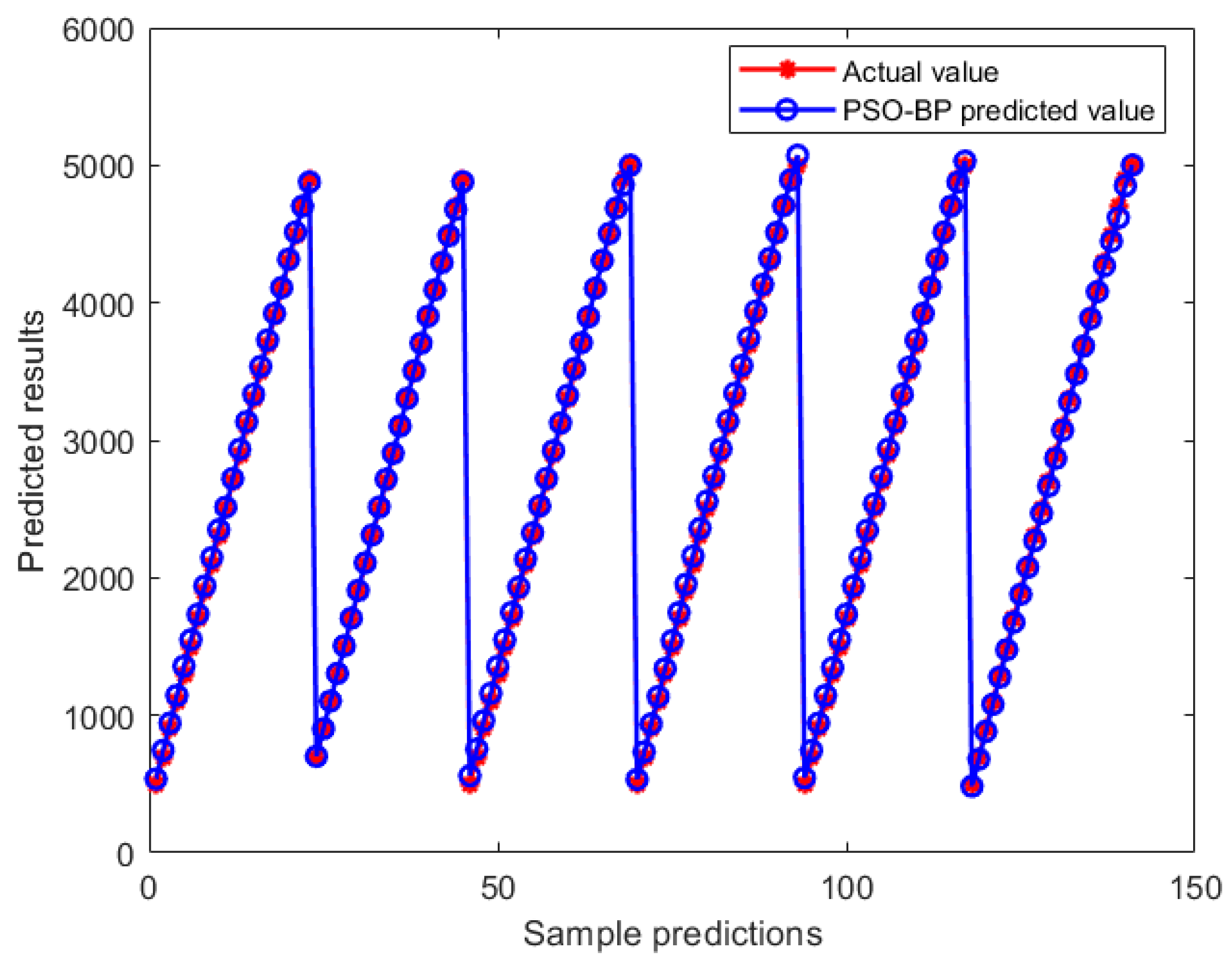
The 120 data sets collected were used as training sets to input the vertical force prediction model. Figure 23 shows the comparison between the predicted results and the true values of the BP neural network vertical force prediction model based on particle swarm optimization. The red line in the figure represents the actual value, and the blue dot line represents the predicted value of the model; through the comparison, it is evident that the vertical force prediction model’s fitting effect on the training set is good. The predicted value almost coincides with the actual value, which shows that the vertical force prediction model can better capture the relationship between input characteristics and target output.
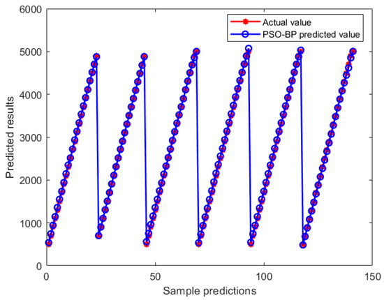
Figure 23.
Comparison of training set prediction.
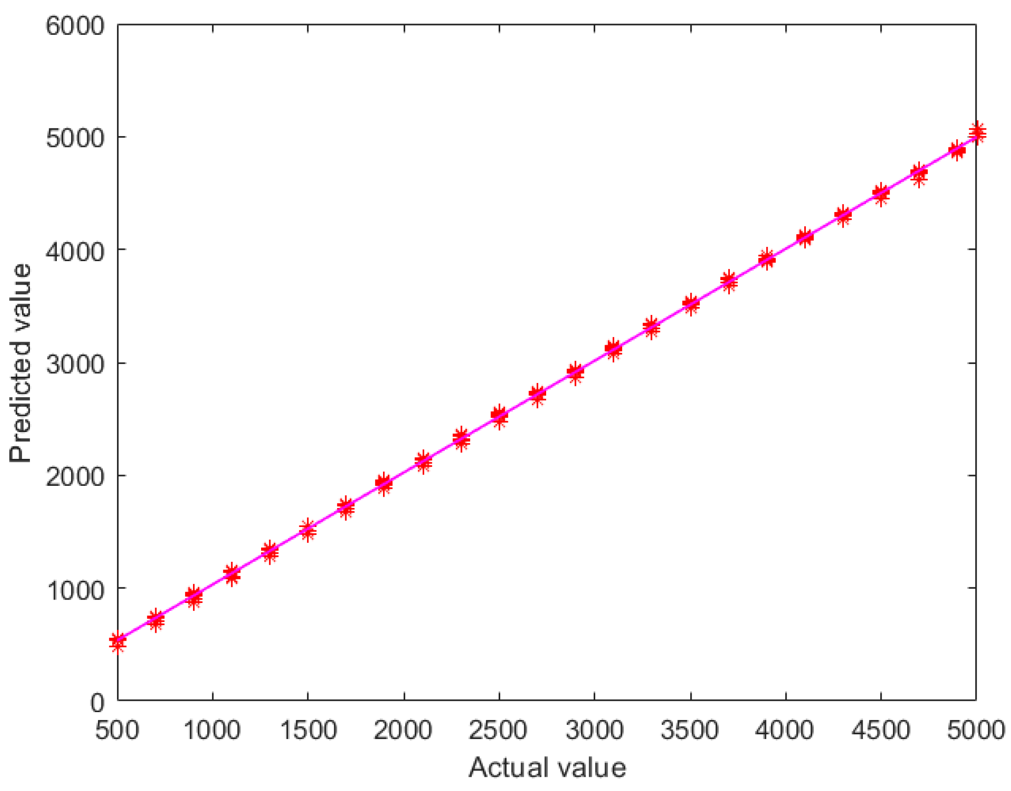
Figure 24 shows the training effect of the BP neural network vertical force prediction model based on particle swarm optimization. In the figure, the abscissa represents the actual value, and the ordinate represents the predicted value. The red symbol in the figure represents the data corresponding to the actual values and predicted values, while the pink line is used to show how the predicted values are distributed and trending overall. The red straight line is close to 45°, with almost no error. The determination coefficient, R2, and root mean square error, RMSE, are the error evaluation indexes of the model output, where the closer the coefficient of determination is to 1, the closer the model’s predictions are to the actual values and the better the fit. Conversely, the smaller it is than 1, the worse the model’s predictions are. The training set coefficient of determination, R2, of the vertical force prediction model is 0.99962, and the root mean square error, RMSE, is 26.3678; thus, the model is well-trained.
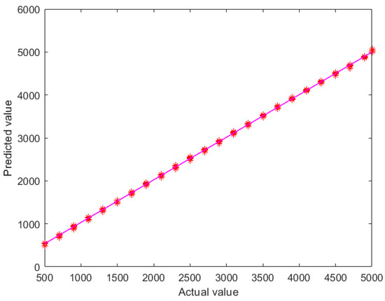
Figure 24.
Training effect diagram.
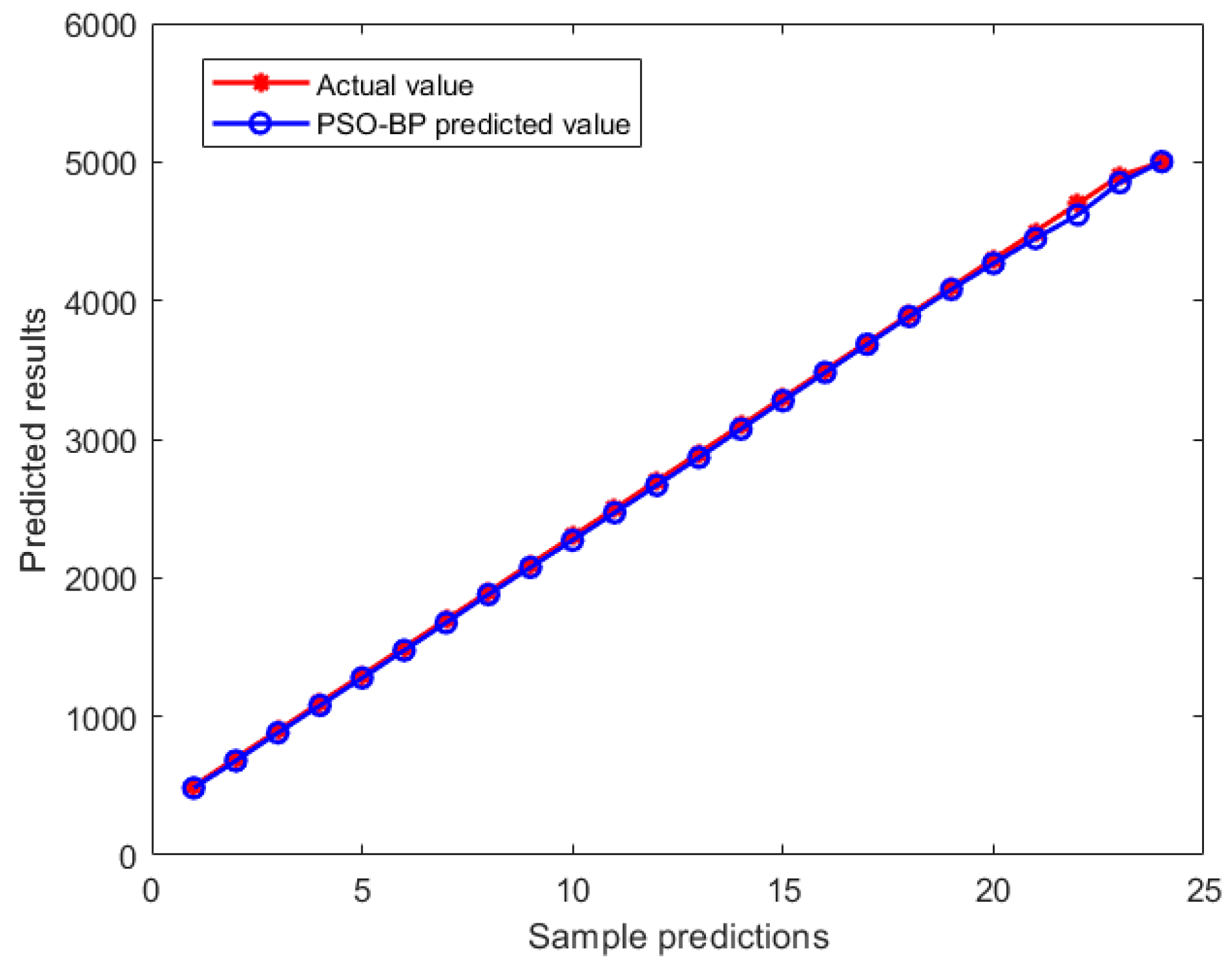
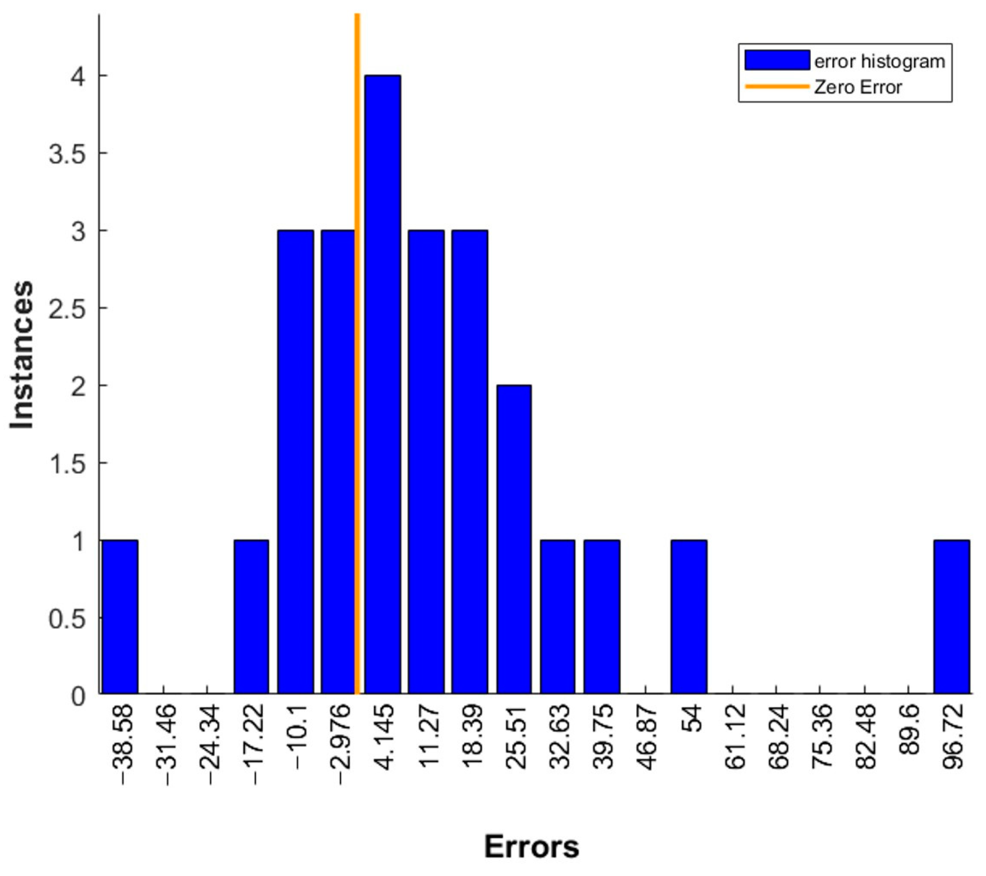
Input the collected 24 groups of data as test sets into the vertical force prediction model. Figure 25, Figure 26 and Figure 27 show the test set results comparison, prediction error histogram, and effect diagram of BP neural network vertical force prediction model based on particle swarm optimization. The error histogram shows the distribution of prediction errors on the test set; it is usually used to check whether there is a significant deviation between the predicted value and the actual value or whether it conforms to some specific distribution rules; if the error distribution is symmetrical, the error is evenly distributed in the positive and negative directions, and is close to zero, which indicates that the prediction result of the model is more accurate if the distribution of errors deviates. It also indicates that there may be some systematic errors in the prediction of the model, which may be higher or lower than the actual value. If the peak value of the histogram is high and concentrated near a specific error value, this shows that most of the error values are concentrated in this range, and the error of the model is relatively consistent; on the contrary, the error distribution is relatively scattered, indicating that the prediction error of the model is relatively scattered, and there may be inaccurate prediction on some samples. The horizontal coordinates in Figure 26 indicate the error values, and the vertical coordinates indicate the frequency of occurrence of each error value. It can be seen that the range of error is concentrated around the zero line, and the range of errors is also mainly concentrated within ±50 and is close to a normal distribution. It means that most of the predicted values are very close to the actual values, the prediction error is small, and the model performs well. It can also be seen that there is some bias in some samples, but the error size of the bias is also only 96.72. Finally, by analyzing Figure 27, the circle symbol in the figure represents the data corresponding to the actual values and predicted values, while the pink line is used to show how the predicted values are distributed and trending overall. We can see that the test set predicted values and the actual values match each other, the test set coefficient of determination R2 of the vertical force prediction model is 0.99955, and the root mean square error RMSE is 29.1858; thus, the model is well trained.
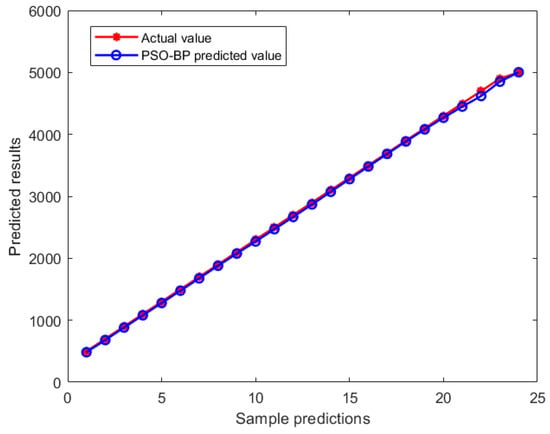
Figure 25.
Comparison of test set prediction results.

Figure 26.
Test set error histogram.
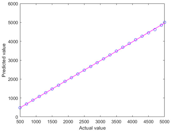
Figure 27.
Test set effect.
5. Conclusions
This paper uses 205/55R16 radial tires as research objects, and the tire grounding parameters and vertical force estimation method were designed using the circumferential strain signal of the inner liner and particle swarm optimization BP neural network algorithm. The main conclusions are as follows:
(1) The average peak spacing angle of the first and second derivative curves of the circumferential strain signal at the centerline of the inner liner of the rolling tire can accurately estimate the contact angle of the rolling tire. When the tire is under acceleration or braking conditions, its grounding characteristics have typical asymmetry, and the length of the contact patch can be effectively estimated by the arc length formula; introducing a correction factor into the arc length formula can reduce the length error between the arc length and the straight line.
(2) The estimation error of a rolling tire’s contact angle and contact patch length under different loads, inflation pressures, road conditions, and slip rates is very small. This shows that the estimation method of rolling tire grounding parameters established in this paper can adapt to different working conditions.
(3) In a characteristic analysis of the circumferential strain signal on the centerline of the inner liner of a rolling tire, there is an apparent linear relationship between the strain signal trough, the trough spacing, and the vertical force; two troughs of circumferential strain signal and a distance between troughs are selected as sensitive characteristic values of vertical force.
(4) The prediction model of rolling tire vertical force based on particle swarm optimization BP neural network can better capture the relationship between input characteristics and target output. The vertical force estimation error is basically within 50 N to realize an accurate estimation of the vertical force of a rolling tire. Different tire patterns, structures, and material parameters can have an impact on the circumferential strain signal, which has little effect on the estimation of ground parameters. However, it will have a certain impact on the vertical force prediction model, and signal data need to be collected again for training and prediction, and the installation position of the strain sensor is important for collecting circumferential strain signals. Meanwhile, during the actual driving process of the vehicle, the collection of strain sensor signals will be affected to some extent by noise, which will have a certain impact on the extraction of circumferential strain signal features. In future work, attention will be paid to solving this problem.
(5) The rolling tire grounding parameters and vertical force estimation method proposed in this article have good estimation effects and can provide accurate inputs for vehicle active safety control systems, which has played a certain role in promoting the development of intelligent chassis technology and the application of intelligent tires. However, this method still has some shortcomings, as it only focuses on the pure longitudinal sliding condition of rolling tires and does not take into account tire side slip and steering conditions. In future work, research will be conducted to address this issue and further improve the universality of this method.
Author Contributions
Article ideas, H.Z., J.Z., Z.J. and G.W.; software: J.Z. and H.L.; experimental verification, J.Z. and H.L.; data analysis, J.Z., H.L. and G.W.; data collection, J.Z. and H.L.; bench, J.Z. and Z.J.; study design, H.Z. and J.Z.; written by J.Z. All authors have read and agreed to the published version of the manuscript.
Funding
Supported by the National Natural Science Foundation of China (Project No. 52272366) and the Postdoctoral Foundation of China (2020M682269).
Data Availability Statement
The raw data supporting the conclusions of this article will be made available by the authors upon request.
Acknowledgments
The author sincerely thanks Haichao Zhou and Zhecheng Jing for their guidance.
Conflicts of Interest
The authors declare no conflicts of interest.
References
- Khaleghian, S.; Emami, A.; Taheri, S. A technical survey on tire-road friction estimation. Friction 2017, 5, 123–146. [Google Scholar] [CrossRef]
- Rajamani, R.; Piyabongkarn, N.; Lew, J.; Yi, K.; Phanomchoeng, G. Tire-Road Friction-Coefficient Estimation. IEEE Control Syst. 2010, 30, 54–69. [Google Scholar] [CrossRef]
- Swami, A.; Liu, C.; Kubenz, J.; Prokop, G.; Pandey, A.K.; Dresden, G.T.U. Germany Experimental Study on Tire Contact Patch Characteristics for Vehicle Handling with Enhanced Optical Measuring System. SAE Int. J. Veh. Dyn. Stab. NVH 2021, 5, 333–350. [Google Scholar] [CrossRef]
- Yuexia, C.; Long, C.; Ruochen, W.; Xing, X.; Yujie, S.; Yanling, L. Modeling and test on height adjustment system of electrically-controlled air suspension for agricultural vehicles. Int. J. Agric. Biol. Eng. 2016, 9, 40–47. [Google Scholar] [CrossRef]
- Liu, H.; Yan, S.; Shen, Y.; Li, C.; Zhang, Y.; Hussain, F. Model predictive control system based on direct yaw moment control for 4WID self-steering agriculture vehicle. Int. J. Agric. Biol. Eng. 2021, 14, 175–181. [Google Scholar] [CrossRef]
- Kongrattanaprasert, W.; Nomura, H.; Kamakura, T.; Ueda, K. Detection of Road Surface States from Tire Noise Using Neural Network Analysis. IEEJ Trans. Ind. Appl. 2010, 130, 920–925. [Google Scholar] [CrossRef]
- Kuno, T.; Sugiura, H. Detection of road conditions with CCD cameras mounted on a vehicle. Syst. Comput. Jpn. 1999, 30, 88–99. [Google Scholar] [CrossRef]
- Wang, Y.; Liang, G.; Gui, Y. Support vector machine based pavement recognition algorithm for smart tyres. Automot. Eng. 2021, 42, 1671–1678. [Google Scholar] [CrossRef]
- Li, J.; Wu, Z.; Li, M.; Shang, Z. Dynamic Measurement Method for Steering Wheel Angle of Autonomous Agricultural Vehicles. Agriculture 2024, 14, 1602. [Google Scholar] [CrossRef]
- Liu, Y.S.; Liu, Z.H.; Gao, Q.H.; Ma, C.Q.; Liu, X.X.; Zhang, J.L. A joint estimation algorithm of vertical force and lateral bias force for heavy-duty tyres based on in-tire strain analysis. J. Beijing Univ. Aeronaut. Astronaut. 2023, 50, 3532–3541. [Google Scholar] [CrossRef]
- Gu, T.; Li, B.; Quan, Z.; Bei, S.; Yin, G.; Guo, J.; Zhou, X.; Han, X. The Vertical Force Estimation Algorithm Based on Smart Tire Technology. World Electr. Veh. J. 2022, 13, 104. [Google Scholar] [CrossRef]
- Wang, Y.; Song, Y.; Wang, Y.; Zhang, J.; He, Z.Z.; Li, Z. Research on the optimization algorithm of off road tire vertical load inversion based on tire circumferential strain. J. Agric. Mach. 2025, 56, 463–473. [Google Scholar] [CrossRef]
- Sun, R.; Wang, Y.; Li, Y.; He, Z.; Zhu, Z.; Li, Z. Parameter identification method of agricultural tire flexible ring model based on particle swarm optimization. J. Agric. Mach. 2024, 55, 402–410. [Google Scholar]
- Erdogan, G.; Alexander, L.; Rajamani, R. Estimation of Tire-Road Friction Coefficient Using a Novel Wireless Piezoelectric Tire Sensor. IEEE Sens. J. 2010, 11, 267–279. [Google Scholar] [CrossRef]
- Xiong, Y.; Yang, X. A review on in-tire sensor systems for tire-road interaction studies. Sens. Rev. 2018, 38, 231–238. [Google Scholar] [CrossRef]
- Xu, N.; Askari, H.; Huang, Y.; Zhou, J.; Khajepour, A. Tire Force Estimation in Intelligent Tires Using Machine Learning. IEEE Trans. Intell. Transp. Syst. 2020, 23, 3565–3574. [Google Scholar] [CrossRef]
- Rajamani, R.; Phanomchoeng, G.; Piyabongkarn, D.; Lew, J.Y. Algorithms for Real-Time Estimation of Individual Wheel Tire-Road Friction Coefficients. IEEE/ASME Trans. Mechatron. 2011, 17, 1183–1195. [Google Scholar] [CrossRef]
- Nishihara, O.; Masahiko, K. Estimation of Road Friction Coefficient Based on the Brush Model. J. Dyn. Syst. Meas. Control 2011, 133, 041006. [Google Scholar] [CrossRef]
- Matsuzaki, R.; Kamai, K.; Seki, R. Intelligent tires for identifying coefficient of friction of tire/road contact surfaces using three-axis accelerometer. Smart Mater. Struct. 2014, 24, 025010. [Google Scholar] [CrossRef]
- Zhou, H.; Li, H.; Yang, J.; Chen, Q.; Wang, G.; Han, T.; Ren, J.; Ma, T. A Strain-Based Method to Estimate Longitudinal Force for Intelligent Tires by Using a Physics-Based Model. Stroj-Vestnik-J. Mech. Eng. 2021, 67, 153–166. [Google Scholar] [CrossRef]
- Li, B.; Quan, Z.; Bei, S.; Zhang, L.; Mao, H. An estimation algorithm for tire wear using intelligent tire concept. Proc. Inst. Mech. Eng. Part D J. Automob. Eng. 2021, 235, 2712–2725. [Google Scholar] [CrossRef]
- Xia, K. Finite element modeling of tire/terrain interaction: Application to predicting soil compaction and tire mobility. J. Terramech. 2010, 48, 113–123. [Google Scholar] [CrossRef]
- Chen, Y.; Chen, L.; Huang, C.; Lu, Y.; Wang, C. A dynamic tire model based on, HPSO-SVM. Int. J. Agric. Biol. Eng. 2019, 12, 36–41. [Google Scholar] [CrossRef]
- Gerthoffert, J.; Cerezo, V.; Thiery, M.; Bouteldja, M.; Do, M.-T. A Brush-based approach for modelling runway friction assessment device. Int. J. Pavement Eng. 2020, 21, 1694–1702. [Google Scholar] [CrossRef]
- Rajendran, S.; Spurgeon, S.K.; Tsampardoukas, G.; Hampson, R. Estimation of road frictional force and wheel slip for effective antilock braking system (ABS) control. Int. J. Robust Nonlinear Control 2019, 29, 736–765. [Google Scholar] [CrossRef]
- Wang, H.; Al-Qadi, I.L.; Stanciulescu, I. Effect of surface friction on tire–pavement contact stresses during vehicle maneuvering. J. Eng. Mech. 2014, 140, 04014001. [Google Scholar] [CrossRef]
- Riehm, P.; Unrau, H.J.; Gauterin, F.; Torbrügge, S.; Wies, B. 3D brush model to predict longitudinal tyre characteristics. Veh. Syst. Dyn. 2019, 57, 17–43. [Google Scholar] [CrossRef]
- Mavros, G.; Rahnejat, H.; King, P.D. Transient analysis of tyre friction generation using a brush model with interconnected viscoelastic bristles. Proc. Inst. Mech. Eng. Part K J. Multi-Body Dyn. 2005, 219, 275–283. [Google Scholar] [CrossRef]
- Li, J.; Cheng, J.; Shi, J.; Huang, F. Brief introduction of back propagation (BP) neural network algorithm and its improvement. In Advances in Computer Science and Information Engineering; Springer: Berlin/Heidelberg, Germany, 2012; Volume 2, pp. 553–558. [Google Scholar] [CrossRef]
- Yu, S.; Zhu, K.; Diao, F. A dynamic all parameters adaptive BP neural networks model and its application on oil reservoir prediction. Appl. Math. Comput. 2008, 195, 66–75. [Google Scholar] [CrossRef]
- Chandio, F.A.; Li, Y.; Xu, L.; Ma, Z.; Ahmad, F.; Cuong, D.M.; Lakhiar, I.A. Predicting 3D forces of disc tool and soil disturbance area using fuzzy logic model under sensor based soil-bin. Int. J. Agric. Biol. Eng. 2020, 13, 77–84. [Google Scholar] [CrossRef]


Disclaimer/Publisher’s Note: The statements, opinions and data contained in all publications are solely those of the individual author(s) and contributor(s) and not of MDPI and/or the editor(s). MDPI and/or the editor(s) disclaim responsibility for any injury to people or property resulting from any ideas, methods, instructions or products referred to in the content. |
© 2025 by the authors. Licensee MDPI, Basel, Switzerland. This article is an open access article distributed under the terms and conditions of the Creative Commons Attribution (CC BY) license (https://creativecommons.org/licenses/by/4.0/).