Abstract
In response to the uncertainty of delay parameters within the servo control system, an adaptive estimation framework grounded in Bayes–Monte Carlo Markov chain fusion (Bayes-MCMC) is proposed. Subsequently, an uncertain delay estimation model was constructed, and a gain optimization method is put forward. An optimal gain state observer tailored to uncertain delays is derived, and a compound control strategy is established to counteract the delay. Experimental findings demonstrate that the observation error of the optimized observer is effectively mitigated. Compared with Smith and the unoptimized gain compensation system, the phase margin, delay margin and gain margin of the system after the gain optimization are increased by 22.8%, 1 order of magnitude, 23.6% and 13.07%, 1 order of magnitude, 1.12%, respectively. Under the condition of delay uncertainty, the system’s output can closely track the given input. The overshoot is effectively reduced, the system’s output response is expedited, the steady-state error is substantially decreased, and the time to reach the steady-state is shortened by around 12.5%. The system’s performance in both the time domain and the frequency domain is remarkably improved, thereby validating the effectiveness and superiority of the proposed method.
1. Introduction
A servo system is a control system designed to accurately track or reproduce a given process, ensuring that the output precisely follows specified changes in quantity. In the domains of industrial automation, robotics, automotive engineering, aerospace, precision machining, and others, a common issue is the presence of a time delay in the servo system of servo motors. This uncertain time delay can result in system instability, degrade the control performance of traditional control strategies, and increase the observation error of observers. This paper investigates the uncertain time delay inherent in the operation of servo systems to ensure they meet stringent precision requirements. In this paper, a high-precision delay estimation module is developed for servo systems with uncertain time delays. Additionally, an adaptive observer gain optimization approach and a composite feedback delay compensation strategy are proposed to reduce the reliance of classical control compensation methods on model accuracy, thereby enhancing the dynamic performance of the system under complex operating conditions.
The Smith predictor, initially proposed by [1] for time delay compensation, transforms time delayed closed-loop systems into delay-free configurations through input delay compensation. However, as demonstrated in subsequent studies [2,3,4,5], its effectiveness crucially depends on precise system modeling, with performance degradation occurring under parameter variations and uncertain delays characteristic of practical servo applications. This limitation motivates our development of an adaptive gain-optimized feedback state observer architecture for enhanced robustness. Bayesian inference demonstrates superior performance in addressing model uncertainty through probabilistic reasoning and adaptive learning mechanisms, having established mature applications across diverse domains including urban water demand forecasting [6], subsurface transportation risk assessment [7], and financial volatility modeling [8,9]. Concurrently, Markov Chain methodologies [10,11,12,13] exhibit exceptional computational efficiency in sampling complex probability distributions, as evidenced by applications in thermal dynamics prediction for water supply systems [10], wind power generation modeling [11], and probabilistic inertia assessment in renewable energy-integrated power grids [12]. The existing literature [14,15,16,17,18,19,20] has documented the integration of Bayesian approaches with Markov chain methodologies, yet systematic investigation into uncertain time delay estimation and modeling for servo systems remains unexplored. For the uncertain time delay of the steering gear servo system, the Bayesian Monte Carlo Markov method is considered for accurate estimation to compensate for the dependence of the classical compensation strategy on the time delay parameters. Aiming at the uncertain time delay compensation of a servo system, according to the estimated uncertain time delay dynamic model, the observer gain is adjusted, and the integrated design of time delay estimation and compensation is constructed to form an adaptive high-precision composite control strategy.
Taking the steering gear servo system with uncertain time delay as the research object, the Bayesian-MCMC and observer gain optimization methods are innovatively proposed to solve two core challenges: (1) Dynamic estimation of uncertain time delay; (2) A gain-optimized feedback observer for uncertain time delay is designed; (3) An adaptive composite control delay compensation strategy is designed. Firstly, the state space expression of the servo system with time delay is listed. Secondly, the time delay estimation module was used to collect the time delay data, and the Bayesian-MCMC was used to accurately model the uncertain time delay. Finally, a composite control strategy combining gain optimization adaptive observer and time delay compensation state feedback is proposed. This method can reduce the observation error while breaking the barrier of time delay uncertainty, and effectively suppress the problem of robustness reduction caused by time delay through compensator design.
2. Problem Description
Using a permanent magnet DC motor as the servo actuator of a steering gear system, and ignoring motor dynamics and nonlinear friction characteristics, the mathematical model of the steering gear servo system with uncertain delay can be obtained as shown in Equation (1).
where is the motor armature current, A; is the armature loop inductance, mh; is the armature circuit resistance, ; is the input armature voltage, V; is the motor output angular speed, ; is the total moment of inertia of motor shaft and load, ; is the viscous damping coefficient; is the Torque coefficient, .
Define the X as shown in Equation (2).
To facilitate the design of the observer, Formula (1) is arranged as follows (3):
Equation (3) is written as a state space equation as Equation (4).
According to state space Equation (4), the system matrix, input matrix, output matrix, and direct transmission matrix can be obtained, as shown in Equation (5) as follows:
said to its derivative feedback effect, reflect in the circuit resistance and inductance of current state suppression. represents the coupling effect of on , reflecting the correlation effect of the motor’s back electromotive force coefficient and inductance on the current . represents the driving effect of on , reflecting the influence of torque coefficient and moment of inertia on mechanical speed . represents the negative feedback effect of on its own derivative, reflecting the attenuation of the mechanical damping coefficient and the moment of inertia on the speed . represents the direct action coefficient of input to , reflecting the transfer relationship of inductance to input voltage. indicates that input has no direct effect on , and the mechanical speed needs to be influenced by input through the electro-mechanical coupling.
The objective of this paper is to design a controller that can adapt to the uncertain time delay of the servo system on the basis of estimating the uncertain time delay, and ensure the fast and stable tracking of the reference signal under the condition of τ(t). According to the controllability and observability criteria in modern control theory, it can be seen that (A,B) is controllable, (A,C) is observable, and the system is affected by uncertain time lag.
3. Uncertain Time Delay Research
3.1. Establishment of Uncertain Time Delay Model
3.1.1. Discussion on Uncertain Delay Types
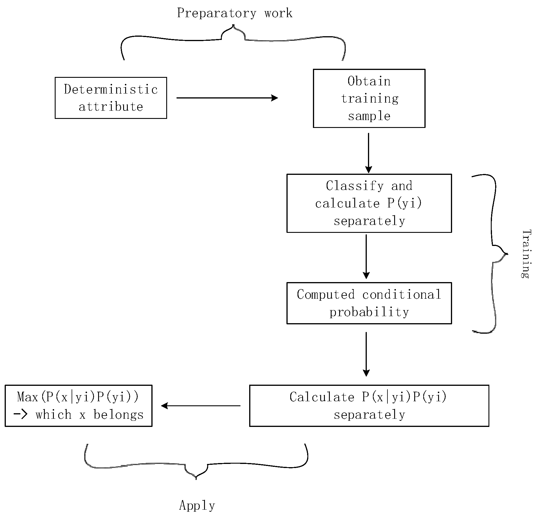
In this paper, we employ the Bayesian method to analyze uncertain delay types within servo systems. Under the assumption that the features of the servo system are mutually independent, we calculate the conditional probabilities of items falling into relevant categories of the servo system for predictive purposes. During the classification process, posterior probabilities of different delay types are compared, and the category with the highest probability is selected as the prediction outcome for uncertain delays. The detailed steps are shown in Figure 1.

Figure 1.
Discussion flow of time delay types.
- ①
- The definition assumes that : The delay parameters of servo system follow normal distribution; The delay parameters follow the white noise distribution completely randomly. The delay parameter of is fixed constant and invariable.
- ②
- Prior probability: To facilitate the calculation of the posterior probability, set .
- ③
- Likelihood function:
For , the likelihood function is based on a normal distribution, where μ is the mean and σ2 is the variance.
For , is based on white noise and the data points are independently and equally distributed.
For , the likelihood function is calculated based on the assumption that the data point is constant.
- ④
- Bayesian analysis:
This paper discusses the types of uncertain delay in the servo system of the steering gear, and preliminarily predicts them to be a normal distribution type and fixed constant type by the Bayesian method.
3.1.2. Time Delay Parameter Model Establishment
The uncertainty delay normal distribution and fixed constant parameters of the servo system estimated in the above section are discussed, and MCMC is proposed.
- (1)
- Estimation of expectation and variance under normal distribution
For the normal distribution type, it is assumed that the prior satisfies conditions , , . Consequently,
For a dataset comprising n observation points, the likelihood function of the entire dataset is expressed as follows:
In accordance with Bayes’ theorem, the posterior distribution satisfies the following relationship:
According to Formulas (6)–(11), the preliminary analysis indicates that the delay distribution conforms to a normal distribution. To estimate the expectation and variance of the delay under this distribution, we employed the Markov Chain Monte Carlo (MCMC) method. Specifically, the sample mean and sample variance were utilized as approximations for the expected value and variance, respectively.
- (2)
- Specific iteration of MCMC
Determine the target posterior distribution and the proposal distribution.
A normal distribution centered on the current sample is usually chosen as the proposal distribution, , where is the variance of the proposal distribution, which needs to be adjusted according to the actual situation. If it is too big, the acceptance rate will be low; however, if it is too small, the Markov chain moves slowly and converges slowly.
Assuming the initial delay value , when time t is reached, the current sample value is , from candidate sample is generated.
Calculate the acceptance probability , since the proposed distribution is a normal distribution, then , so
Generate a uniformly distributed random number , if , then , otherwise , and repeat the above iterative process until the Markov chain converges, setting the scaling factor.
Set the number of iterations to 10,000 times and sort out the resulting τ value.
According to the collected data, because of the huge amount of data, the combination of Formulas (9)–(14) was used for computer analysis. We combine Bayes and Algorithm 1 in this part and get the estimated delay as τ(t).
Finally, the estimated delay τ(t)~N(0.47333,6.4662) was obtained, and the estimated delay model distribution was used as the simulation delay to build the simulation system.
| Algorithm 1 MCMC Process | |
| 1 | iter = 0 |
| 2 | while (iter < 10000): |
| 3 | //tau_star <- candidate_example |
| 4 | //u <-random_number_ between_0_and_1 |
| 5 | calculate_prior_tau_star_value |
| 6 | calculate_prior_tau_current_value |
| 7 | calculate_likelihood_function_value_at_tau_star and tau_current |
| 8 | calculate_acceptance_probability(tau_current, tau_star) |
| 9 | if (u <= accept_prob): |
| 10 | tau_current = tau_star |
| 11 | tau_samples[iter] = tau_current |
| 12 | iter = iter + 1 |
| 13 | mu_p = calculate_average_of_tau_samples_array |
4. Delay Compensation System Design
4.1. Structure of Time Delay Compensation System
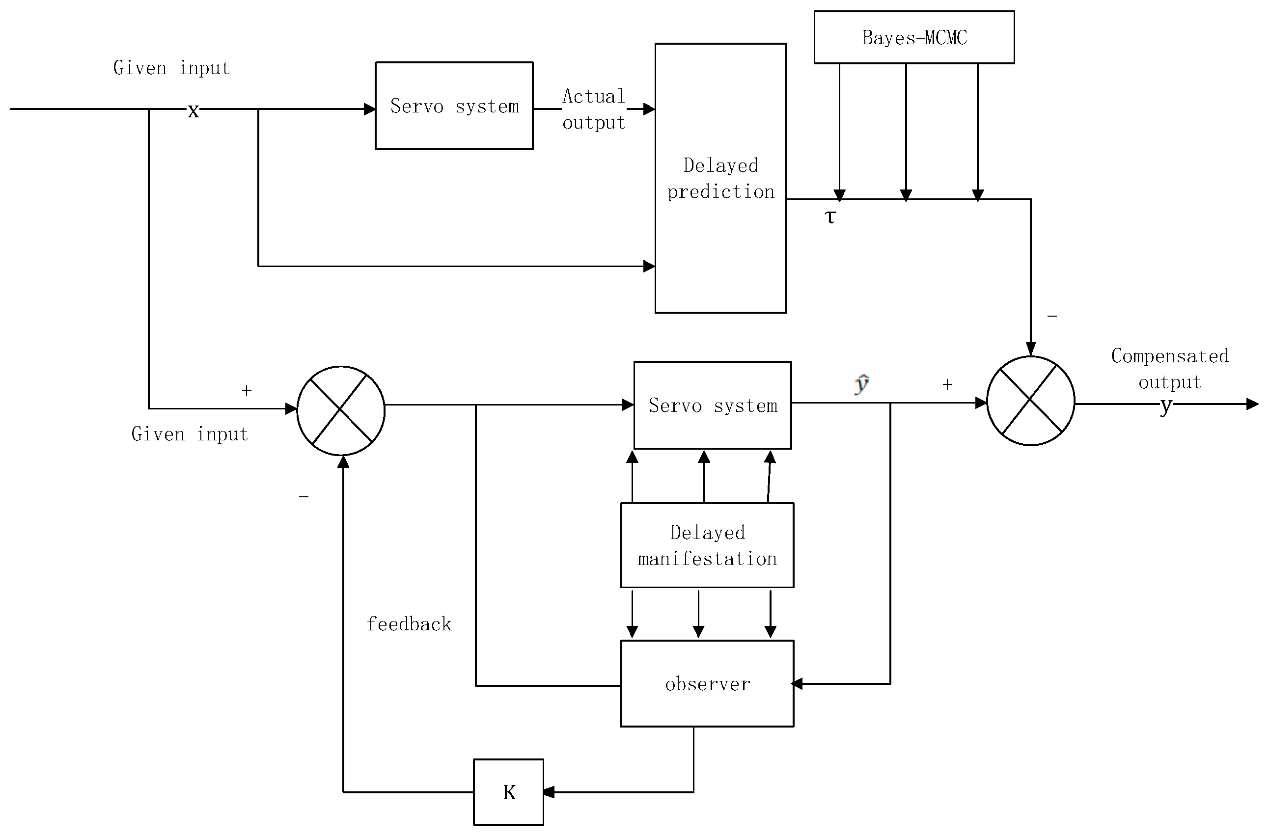
In Section 3, the Bayesian MCMC method has been used to estimate and model the uncertain delay based on the collected data of the servo system. As shown in Figure 2, the time delay compensation system is studied and analyzed in Section 4.
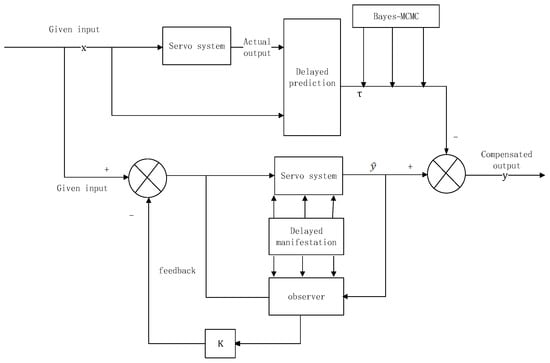
Figure 2.
Structure diagram of time-delay compensation system.
The dependence relation makes the time-delay system mathematically modellable as an infinite-dimensional system [21]. However, in the actual system analysis and controller design, the infinite-dimensional model is more complex, so it is necessary to find a method to convert the infinite-dimensional system into an equivalent finite-dimensional system. An innovative strategy for optimizing and adjusting the system matrix is proposed. This strategy introduces a time delay term and explicitly constructs a new state space model that can reflect the dynamic influence of time delay on the system. The adjusted new symmetric matrix was used to calculate the observer gain and feedback matrix, so that the observer can better perform state estimation in the presence of time delay, and the composite control compensation strategy can better perform time delay compensation.
4.2. Delayed Prediction
In Formula (15), where is the signal to be analyzed, is the reference signal, and represents the time delay, representing the delay of the signal relative to , stands for normalized cross-correlation values. The closer the normalized cross-correlation value is to 1, the higher the similarity between the two signals at the delay . We apply Algorithm 2 to this part.
| Algorithm 2 Delayed Prediction | |
| 1 | Function estimate_delay(x, d) |
| 2 | Input: |
| 3 | x: Input signal |
| 4 | d: Reference signal |
| 5 | Calculate the cross-correlation between input signal x and reference signal d |
| 6 | Find the maximum of the absolute value of the cross-correlation function |
| 7 | Estimate the delay |
| 8 | Obtain the cross-correlation peak value |
| 9 | correlation_peak |
| 10 | Return the result |
| 11 | End function |
4.3. Gain Optimization Feedback State Observer
The state equation of a state observer [22] with feedback is as follows:
when the uncertain delay exists, becomes equation .
After delay manifestation, the equation of state becomes the following:
The observer state equation for compensating time lag is simplified to Equation (18).
Next, judge the convergence of the observer.
In order to ensure the asymptotic stability of the system, must be negative definite. Combined with a series of derivations, the Formula (20) can be obtained.
At the same time, in order to ensure the positive definiteness of the functional, then . Under this condition, if all LMI constraints are satisfied, the observer is asymptotically stable.
The transformation of the system state Equation (3) with time delay can obtain the poles of the system as follows (21):
According to Routh criterion, the real part of all eigenvalues is negative and the original system is asymptotically stable.
For each eigenvalue, set .
The transformation of matrix gives ,
V is the eigenvector matrix of the system matrix A, is the eigenvalue of A, and the uncertain delay is estimated, and represents the real part of the eigenvalue.
Thus, a new equation of state of the system is obtained.
After the transformation, the poles of the delay servo system are changed into Formula (28).
The system is still asymptotically stable after delay manifestation.
In comparison, it is evident that as the absolute value of the real part of the pole increases, the response of the servo system decays to the theoretical value more rapidly, thereby effectively mitigating the impact of time delay on the dynamic performance of the servo system to a significant extent.
To address the uncertain time delay issue inherent in the steering gear’s servo system, this paper proposes a method for determining observer parameters based on the adjusted system matrix and introduces a time delay compensation approach. Consequently, the controller can preemptively respond before experiencing actual time delay, ensuring the system maintains optimal performance even under time delay conditions.
We apply Algorithm 3 to this part. Based on the new state equation after delay manifestation, the observer matrix and feedback matrix are obtained by setting appropriate Q and R, as shown in Equation (33).
| Algorithm 3 Gain Optimization | |
| 1 | Input: |
| 2 | Q: Status weight |
| 3 | R: Control weight |
| 4 | System matrix A, B, C |
| 5 | Function design_compensator(A, B, C, tau, Q, R): |
| 6 | set the matrix(A, B, C, Q, R, tau) |
| 7 | //Judge the observability and controllability of system |
| 8 | If the system (A, B, C) is not observable or not controllable then |
| 9 | Print “The system is either unobservable or uncontrollable”. |
| 10 | Return null |
| 11 | End If |
| 12 | Calculate V and D from A |
| 13 | Calculate the eigenvalues and eigenvectors of the system |
| 14 | Delayed manifestation: |
| 15 | //V is the eigenvalue of A, D is the eigenvector of A |
| 16 | Calculate the adjusted system matrix A_hat: |
| 17 | A_hat = V*diag(λ_i + τ*max(Re(λ_i)))*V^’ |
| 18 | //λ_i <- Diagonal elements of D |
| 19 | //Re(λ_i) <- Take the real part of λ_i |
| 20 | //max(Re(λ_i)) <- Find the maximum value of the real part of the diagonal element |
| 21 | //diag(W) <- Extract the diagonal elements of matrix W |
| 22 | //V^’ <- V transpose |
| 23 | Design observer gain matrix L0 |
| 24 | Design LQR controller |
| 25 | Construct the observation error system |
| 26 | Define the LMI variable |
| 27 | Construct Lyapunov-Krasovskii functional dependent LMI constraints |
| 28 | Solving LMI |
| 29 | Judge observer stability |
| 30 | return L,K |
5. Experimental Verification
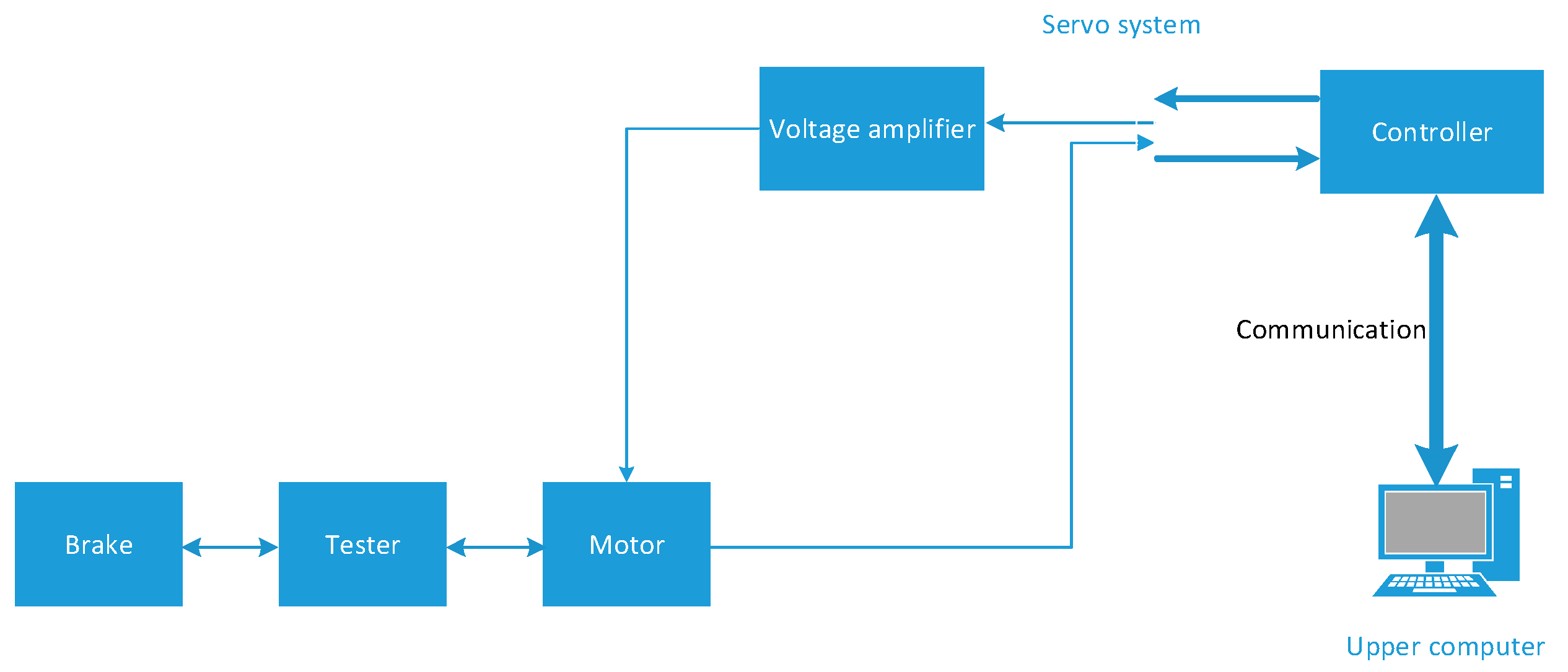
In order to verify the effectiveness of the control algorithm proposed in this paper, the above simulation was implemented on the servo motor drive control platform. The schematic diagram and the actual object of the servo motor drive control platform are shown in Figure 3 and Figure 4, respectively. The experiment builds the control algorithm through MATLAB R2024a/Simulink and adopts CCS 9.1.0 programming. DSP TMS320F28377D was used to realize the development and application of servo drive control of motor. The TMS320F28377D has dual-core cpus, each 32-bit, 200 MHz, equipped with floating-point units, TMU\VCU-11, and two CLAs.
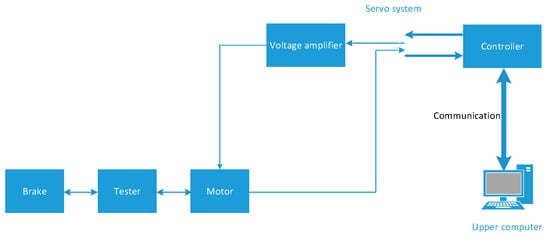
Figure 3.
Servo motor drive control platform.

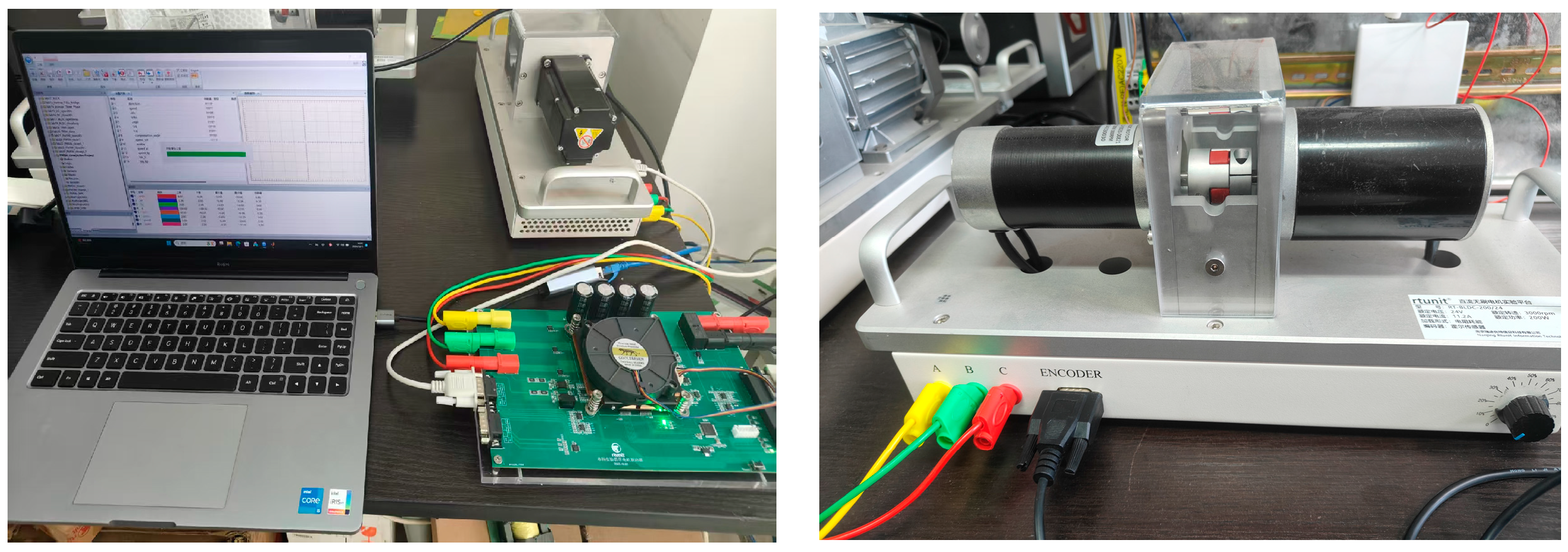
Figure 4.
Physical diagram of the experimental platform.
MOTOR: KIZI BLDC MOTOR
57BL115-Y30220-D0821
Sensor: LEM’s Hall current sensor LAH25-NP
The device parameters are shown in Table 1.

Table 1.
Servo system platform parameter Settings.
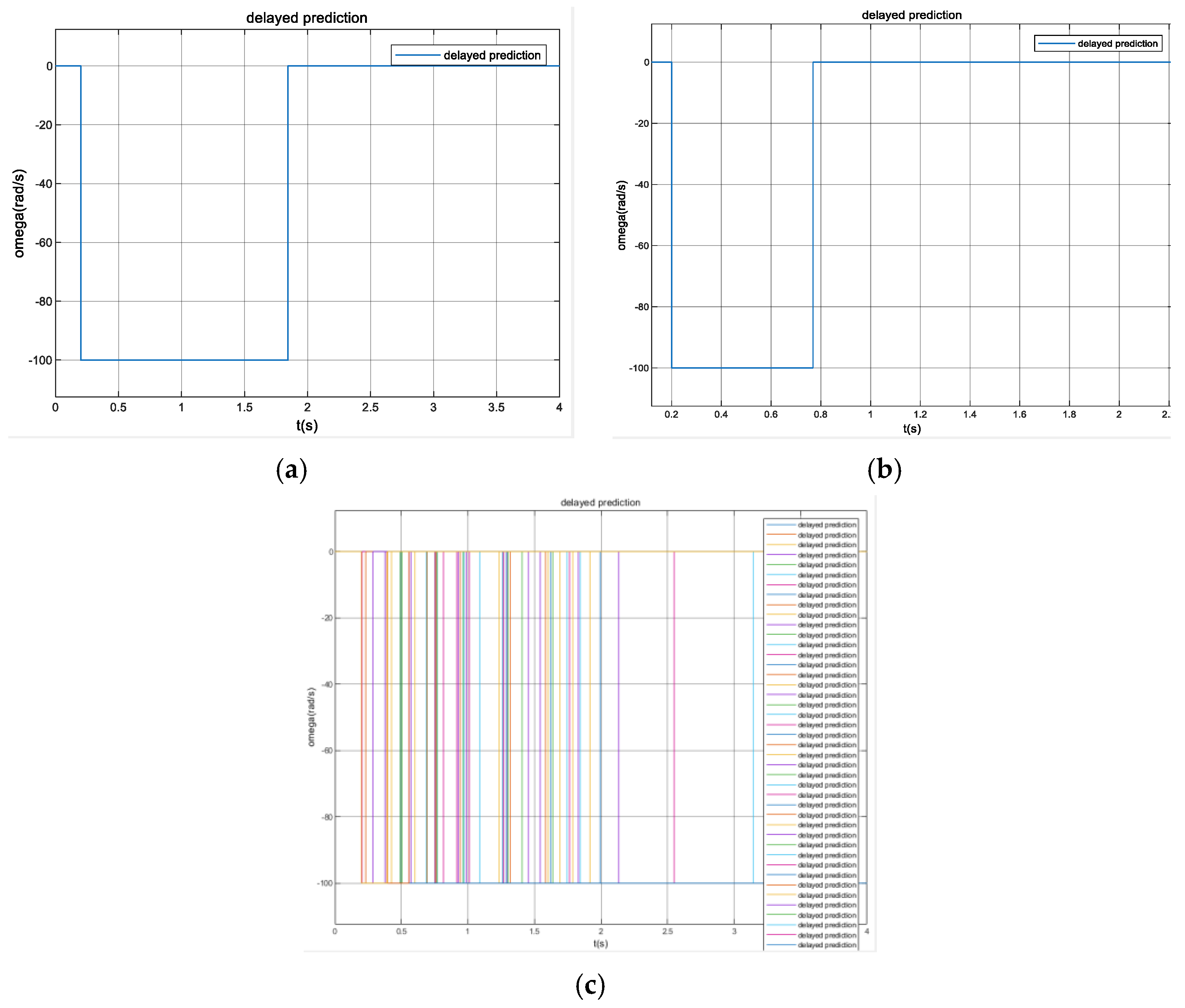
According to the given input and actual output response time, 100 groups of delay data are estimated to draw waveforms as shown in Figure 5.
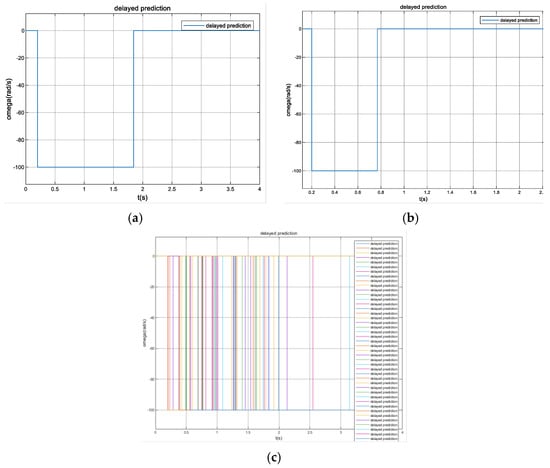
Figure 5.
Estimated time delay parameter data presentation: (a) Tau = 2.6438; (b) Tau = 0.5682; (c) More than 100 sets of time-delay data acquisition (Presentation section).
6. Analysis and Comparison of Experimental Results
6.1. Time Domain Analysis of System Response
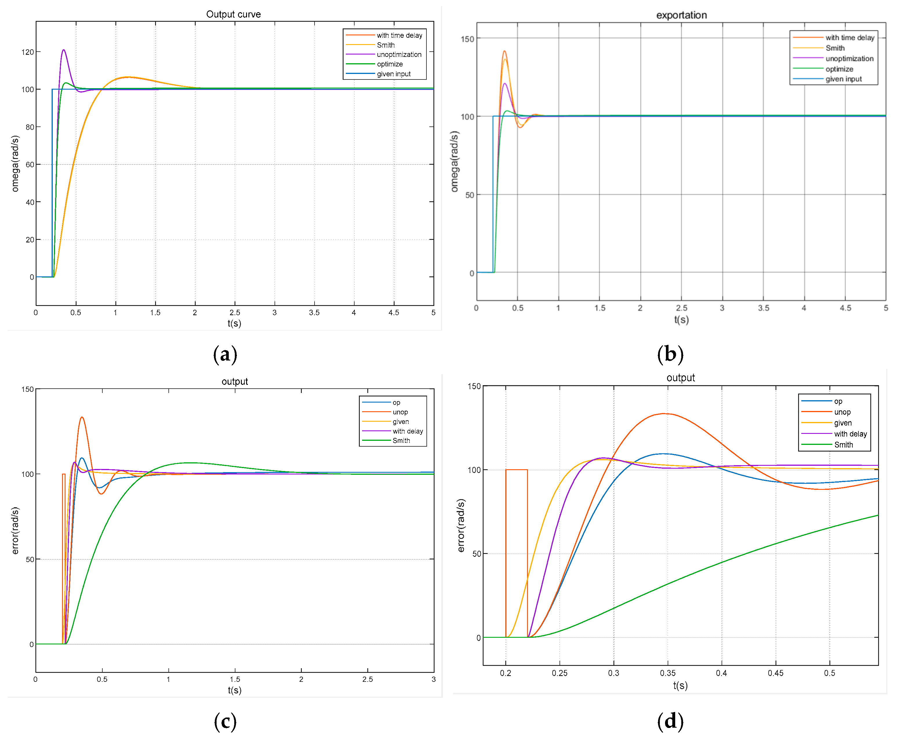
The time-domain angle of the control servo system before compensation and the proposed control compensation method were analyzed and compared, as shown in Figure 6.
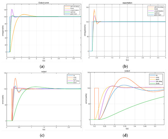
Figure 6.
The output comparison diagram with the same delay parameter: (a) Adjust the output comparison under different PID parameters; (b) Adjust the output comparison under the same PID parameters; (c) Change lag output comparison diagram; (d) Output (c) enlarged image.
From the perspective of overshoot analysis and comparison, under the time delay condition, as shown in Figure 6a,b, the output curve shows a significant peak before reaching a steady state, showing a large overshoot. Before gain optimization, the compensated time delay systems showed reduced output fluctuations and overshoot decreases by 13.2% and 12.5%, respectively, compared with the uncompensated state. Compared with Smith, the output curve overshoot after gain optimization is reduced by about 2.7% and 19.2%, respectively.
Analysis of Figure 6c,d shows that the uncompensated system shows a significant response delay after the input step change. The lag phenomenon is obviously weakened by time delay compensation.
This optimization strategy has obvious advantages in enhancing system responsiveness, effectively suppressing overshoot and significantly reducing steady-state error. The improvement of comprehensive performance verifies its technical advantages.
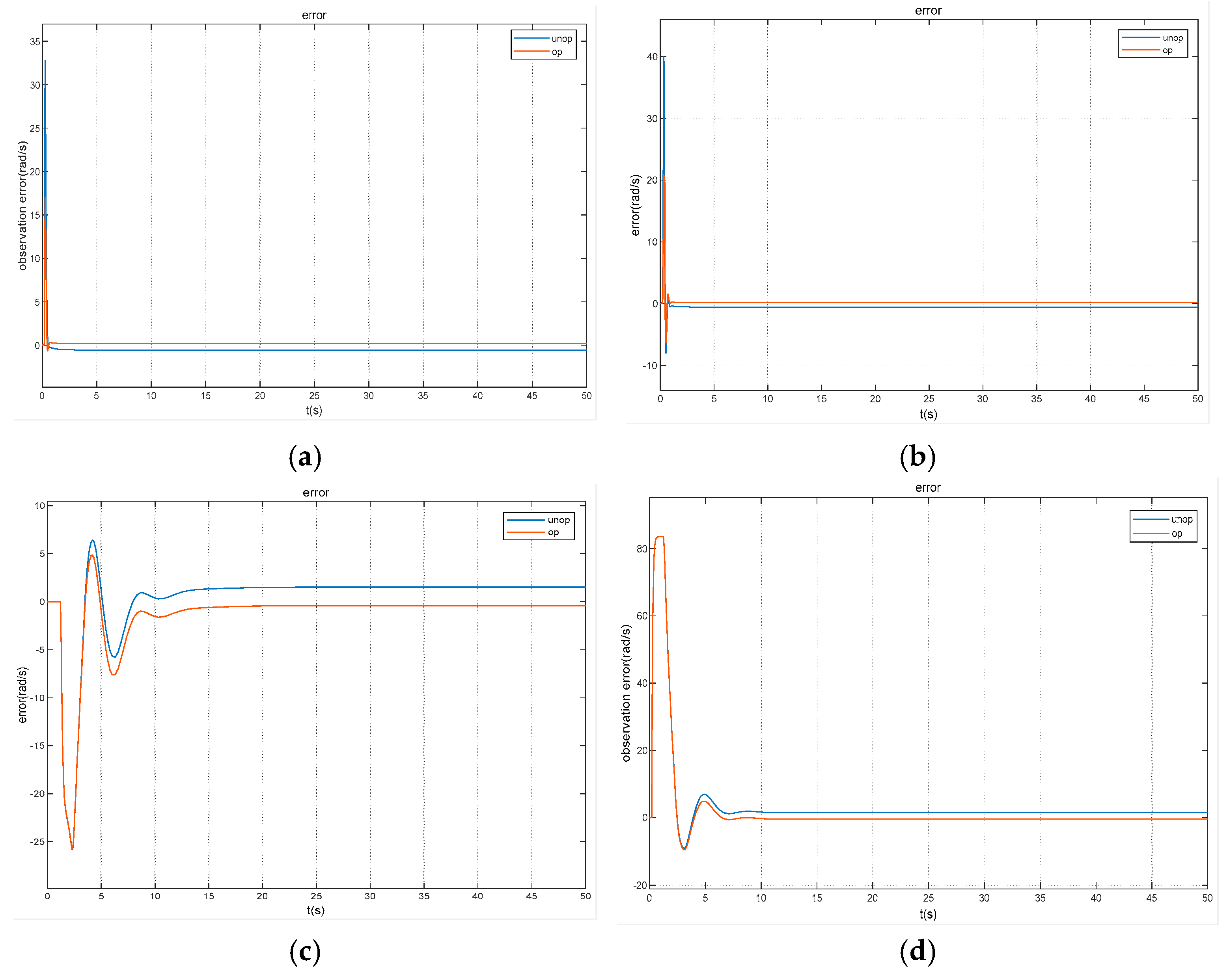
By comparing the observation errors of the observer before and after gain optimization, the simulation results of the observation errors are shown in Figure 7 and Figure 8 respectively when the input is a step signal and a sinusoidal signal.
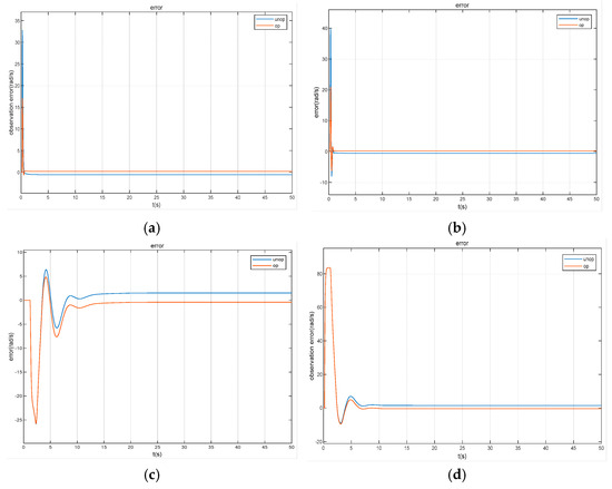
Figure 7.
Comparison of observation errors under different time-delay parameters with step input: (a) Tau is 0.0206, x-xhat; (b) Tau is 0.0206, y-yhat; (c) Tau is 1.321, x-xhat; (d) Tau is 1.321, y-yhat.
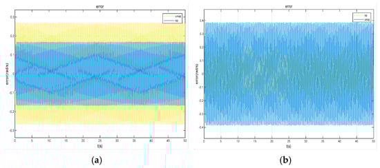
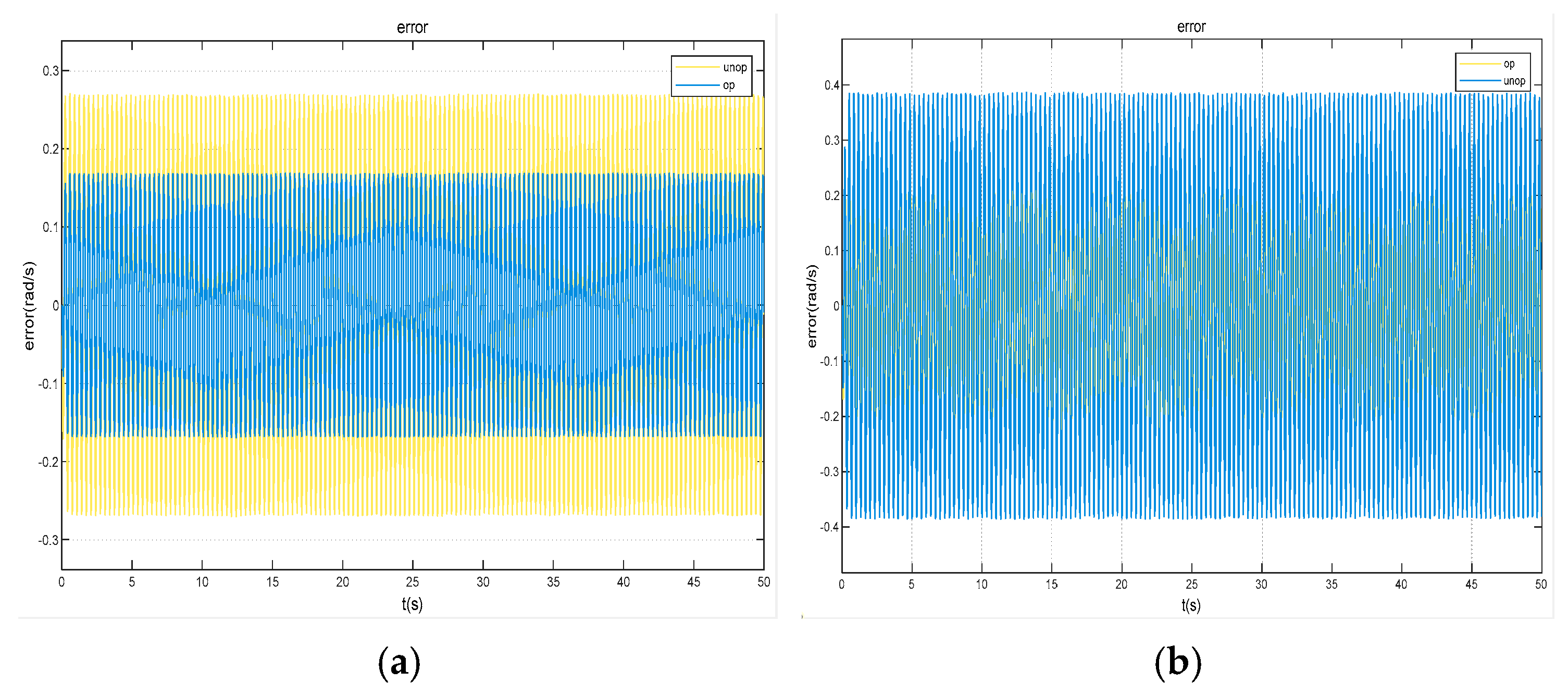
Figure 8.
Comparison of observation errors under different time delay parameters of chord wave input: (a) Tau is 0.0206, x-xhat; (b) Tau is 0.0206, y-yhat.
According to the comprehensive comparative analysis shown in Figure 7 and Figure 8, when there is a time delay, the observation error of the observer optimized by the time delay representation principle is effectively reduced by 33.3% and the observation error of y is effectively reduced by 42.1%, and the observation value is more accurate.
6.2. Frequency Domain Analysis of System Response
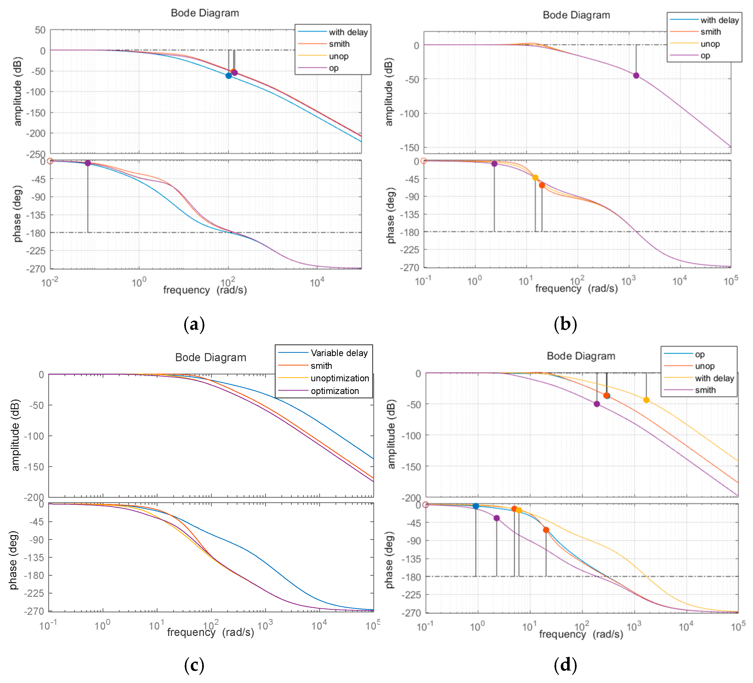
The compensation system is built according to the estimated delay parameters, and the Bode diagram under different delay conditions is drawn, as shown in Figure 9.
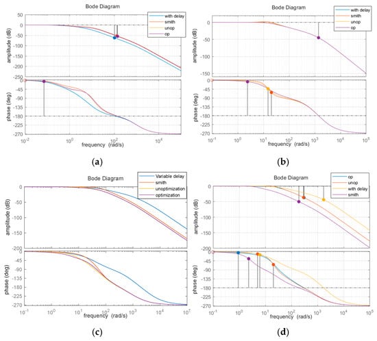
Figure 9.
Bode diagram: (a) Tau is 1.321; (b) Tau is 0.0206; (c) Delay stochastic; (d) Delay stochastic.
As shown in Figure 9c,d, when the time-varying delay is used to simulate the actual time delay deviating from the prior, the Smith compensation effect is quite poor, while the composite control compensation strategy proposed in this paper still maintains a high compensation accuracy.
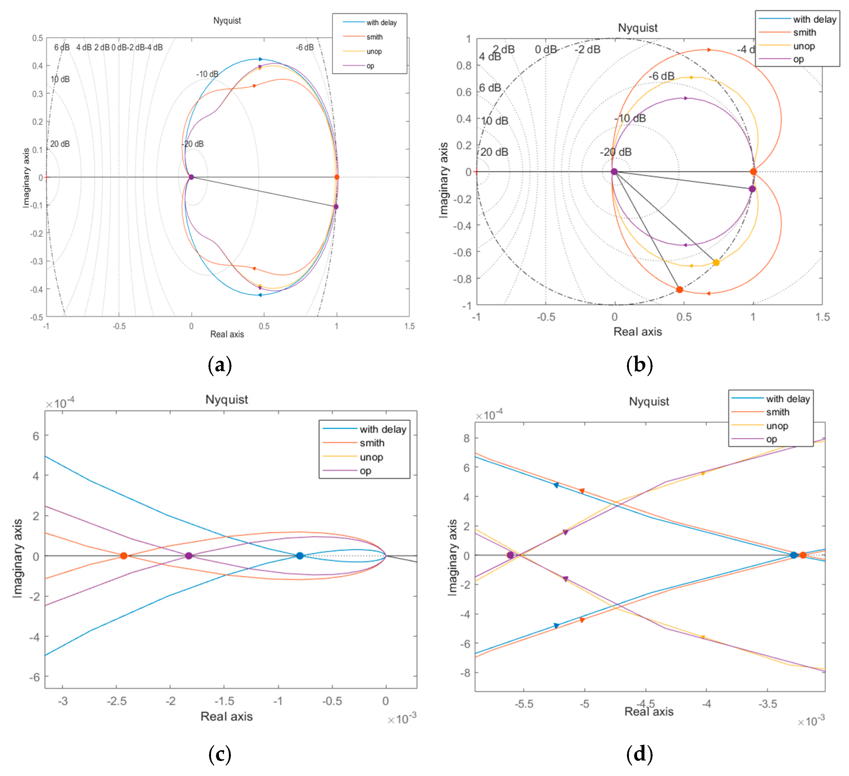
Extract important features from the Bode chart shown in Figure 9 and Figure 10 and list the data as shown in Table 2.
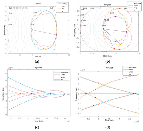
Figure 10.
Nyquist: (a) tau is 1.321; (b) tau is 0.0206; (c) a partial enlarged view of Figure (a); (d) partial enlarged view of Figure (b).
Table 2.
Comparison of Bode Chart curve characteristic records before and after compensation.
The critical parameters of the Bode plot before and after compensation were analyzed and compared, with a comprehensive evaluation of the delay margin, phase margin, and gain margin. The delay margin is particularly significant in practical applications because each component in real-world control systems introduces time delays that can severely compromise system stability. A larger delay margin indicates greater tolerance to these delays, thereby enhancing the system’s stability and robustness. After Smith compensation, the delay margin remains nearly unchanged. In contrast, the delay margin increases by 228% following feedback state observer compensation compared to pre-compensation levels, and it increases by an order of magnitude after gain optimization compensation relative to non-optimized conditions. This suggests that the system exhibits higher tolerance to time delays and improved stability and robustness.
The phase margin increased by 13.07% after gain optimization compensation compared to pre-optimization levels, indicating enhanced tolerance to phase changes post-optimization. This improvement effectively reduces phase lag within the system and optimizes the phase characteristics of the closed-loop system at the cutoff frequency. The enhanced phase margin not only improves the system’s adaptability to parameter perturbations but also ensures sufficient stability margins in the frequency domain, which is crucial for suppressing high-frequency oscillations.
Following gain optimization compensation, the gain margin increased by 1.12% compared to pre-optimization levels, expanding the stable operating range of the system. An increase in gain margin implies that the critical point of open-loop gain shifts to a higher frequency band, translating into stronger resistance to gain disturbances in practical applications.
These experimental results demonstrate that the proposed gain optimization method enables the controller to anticipate responses without experiencing actual time lags, maintaining optimal performance even under time delayed conditions.
7. Conclusions
This study investigates adaptive control strategies for servo systems operating under uncertain time delay conditions. To address the challenge of delay uncertainty, we developed a probabilistic framework integrating Bayesian inference with Markov Chain Monte Carlo (MCMC) simulations, enabling robust parameter estimation and uncertainty quantification. Building upon the transformed state-space representation of servo dynamics, we propose a novel delay-compensation mechanism through an adaptive observer-based framework that systematically integrates optimized state variables with time delay characteristics.
Experimental validation reveals substantial performance improvements through our compensation strategy. The proposed methodology offers three key contributions: (1) A systematic approach for uncertainty modeling in time delay systems; (2) An observer-based compensation framework featuring optimized gain adaptation; (3) Quantifiable evidence of performance enhancements in both temporal and spectral domains. These findings highlight the practical applicability of our approach in industrial automation scenarios where time delay uncertainties significantly impact control stability and observation accuracy, while establishing a novel optimization pathway for complex system design through probabilistic modeling and adaptive compensation techniques.
Author Contributions
Methodology, M.M.; Software, M.M.; Data curation, W.M.; Writing—original draft, M.M.; Writing—review & editing, M.M.; Visualization, M.M.; Project administration, S.Y.; Funding acquisition, S.Y. All authors have read and agreed to the published version of the manuscript.
Funding
This research received no external funding.
Data Availability Statement
The original contributions presented in this study are included in the article. Further inquiries can be directed to the corresponding author.
Conflicts of Interest
The authors declare no conflict of interest.
References
- Han, J.Q. Self-Tuning Anti-Disturbance Control for Time-Delay Objects. Control Eng. 2008, S2, 7–10+18. [Google Scholar]
- Tao, L.; Chen, S.; Fang, G.; Zu, G. Smith Predictor-Taylor Series-Based LQG Control for Time Delay Compensation of Vehicle Semiactive Suspension. Shock Vib. 2019, 2019, 1–12. [Google Scholar] [CrossRef]
- Nie, Y.; Zhang, P.; Cai, G.; Zhao, Y.; Xu, M. Unified Smith predictor compensation and optimal damping control for time-delay power system. Int. J. Electr. Power Energy Syst. 2020, 117, 105670. [Google Scholar] [CrossRef]
- Fan, Y.S.; Luo, E.Y.; Wang, G.F. Simulation of Position Control of Pneumatic System Based on Time-Delay Compensation. Sci. Technol. Eng. 2021, 21, 10680–10689. [Google Scholar]
- Ji, J.B.; Xu, J.C.; Wang, D.Y. Research on Sub-Structure Test Method of Vibration Table Based on Improved Smith Predictor. Mach. Tool Hydraul. 2024, 52, 14–21. [Google Scholar]
- Chen, L. Probability Prediction of Daily Water Consumption Based on Bayesian Theory. Syst. Eng. Theory Pract. 2017, 37, 761–767. [Google Scholar]
- Song, J.W.; Zhang, S.; Li, K.X. Adaptive Bayesian Model Updating Method with Variable Observation Domain. J. Beihang Univ. 2025, 1–13. [Google Scholar] [CrossRef]
- Shang, T.; Guo, M.Y.; Tang, B.M.; Xu, Y.T. Driving Risk Assessment of Underground Roads Based on Dynamic Bayesian Network. Transp. Syst. Eng. Inf. 2025, 1–22. [Google Scholar]
- Wang, C.X.; Wang, R.Q. Short-Term Trend Prediction Model of Stock Market Based on Pattern Recognition and Bayesian Decision-Making. Stat. Decis. 2024, 40, 154–158. [Google Scholar] [CrossRef]
- Yuan, X.Y.; Zhao, Y.D. Prediction of Water Supply Temperature in Heat—Exchange Station Based on Grey Markov Chain Prediction Model. Electron. Meas. Technol. 2015, 38, 32–34. [Google Scholar] [CrossRef]
- Zhu, C.X.; Zhang, Y.; Yan, Z.; Zhu, J.; Zhao, T. Modeling of Wind Power Sequence Using Improved Markov Chain Monte Carlo Method. Trans. China Electrotech. Soc. 2020, 35, 577–589. [Google Scholar] [CrossRef]
- Wang, Q.Q.; Yao, L.Z.; Xu, J.; Cheng, F.; Mao, B.; Wen, Z.; Chen, R. Probabilistic Assessment of Equivalent Inertia of High—Proportion Renewable Energy Power Systems Based on Slice Sampling—Markov Chain Monte Carlo Simulation. Power Syst. Technol. 2024, 48, 140–152. [Google Scholar] [CrossRef]
- Ye, L.; Jiang, H.K.; Zou, Y.Q.; Chen, H.P.; Wang, L.P. Bayesian Finite Element Model Updating Based on Markov Chain Population Competition. J. Mech. Strength 2025, 85–93. [Google Scholar]
- Miao, H.; Guo, W.L.; Liu, Z.Y.; Wang, R.J. Ultraviolet LED Lifetime Prediction Based on Bayesian MCMC and Other Models. Acta Opt. Sin. 2024, 44, 170–177. [Google Scholar]
- Padilla, G.J.L.; Azevedo, C.L.; Lachos, V.H. Parameter recovery of skew multidimensional multiple-group item response models (MGM-MIRT): A comparison of MCMC algorithms and assessment of effects of interest. J. Stat. Comput. Simul. 2025, 95, 467–489. [Google Scholar] [CrossRef]
- Chen, H.G.; Xu, L.L.; Tang, X.Q. Implicit Markov HDP Non-Parametric Bayesian Video Anomaly Detection. Control Eng. 2019, 26, 1763–1769. [Google Scholar] [CrossRef]
- de Oliveira, J.T.; de Carvalho Costa, L.R.; Estumano, D.C.; Féris, L.A. Applying Bayesian statistics and MCMC to ozone reaction kinetics: Implications for water treatment models. Chemosphere 2025, 373, 144164. [Google Scholar]
- Miao, J.; Duan, L.; Liu, J.M.; Lin, S.W.; Zhao, J.C. Structural Simulation Model Updating Based on Improved MCMC Method and Surrogate Model. J. Shanghai Jiao Tong Univ. Sci. 2025, 67, 1–17. [Google Scholar] [CrossRef]
- Arabpour, A.; Moghadam, H.R.; Niri, E.M. Geophysical bayesian inverse problem solving with tuning-free adaptive MCMC sampler. Earth Sci. Inform. 2025, 18, 186. [Google Scholar]
- Wang, L.Y.; Xi, C. An Improved MCMC Algorithm for Inverting Source Parameters Using GPS Data in Bayesian Framework. Chin. J. Geophys. 2024, 67, 3367–3385. [Google Scholar]
- Hu, J.M.; Liu, W.; Yan, F.; Hu, Y.J. Robust Optimal Reinsurance and Investment Strategies with Time-Delay under the Mean-Variance Premium Principle. Chin. J. Eng. Math. 2024, 41, 1–16. [Google Scholar]
- Chang, X.H.; Pan, T.T.; Xiong, J. A New Method for the Analysis and Design of State Observers. J. Jilin Norm. Univ. Nat. Sci. Ed. 2024, 45, 53–61. [Google Scholar]
Disclaimer/Publisher’s Note: The statements, opinions and data contained in all publications are solely those of the individual author(s) and contributor(s) and not of MDPI and/or the editor(s). MDPI and/or the editor(s) disclaim responsibility for any injury to people or property resulting from any ideas, methods, instructions or products referred to in the content. |
© 2025 by the authors. Licensee MDPI, Basel, Switzerland. This article is an open access article distributed under the terms and conditions of the Creative Commons Attribution (CC BY) license (https://creativecommons.org/licenses/by/4.0/).