
Numerical and Experimental Investigation of the Ultra-Low Head Bidirectional Shaft Extension Pump Under Near-Zero Head Conditions

Abstract
1. Introduction
2. Numerical Simulation and Experimental Setup
2.1. Governing Equations and Cavitation Model
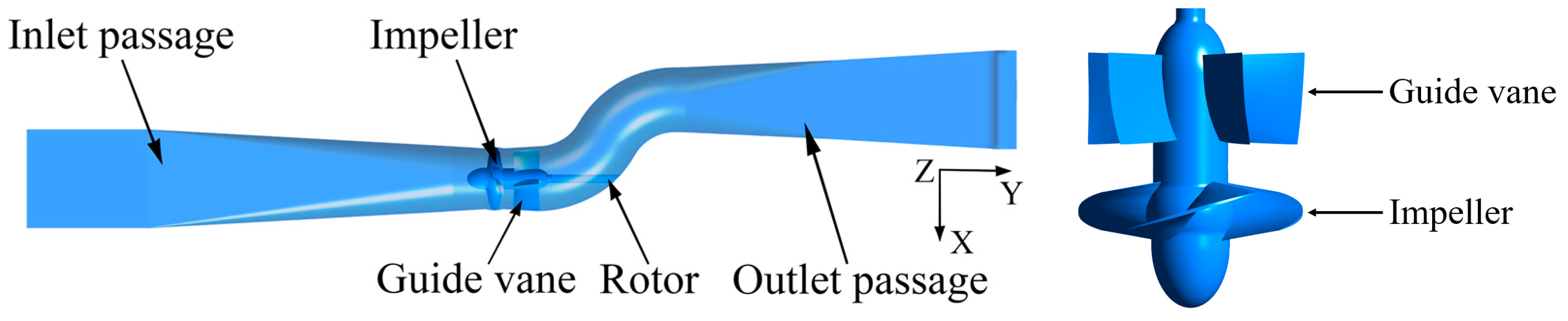
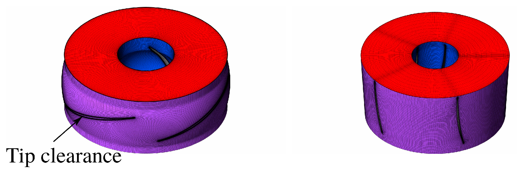
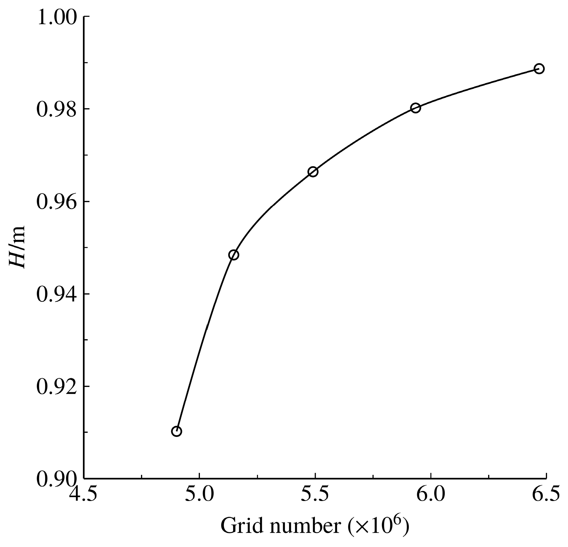
2.2. Computational Domain, Mesh, and Numerical Setup
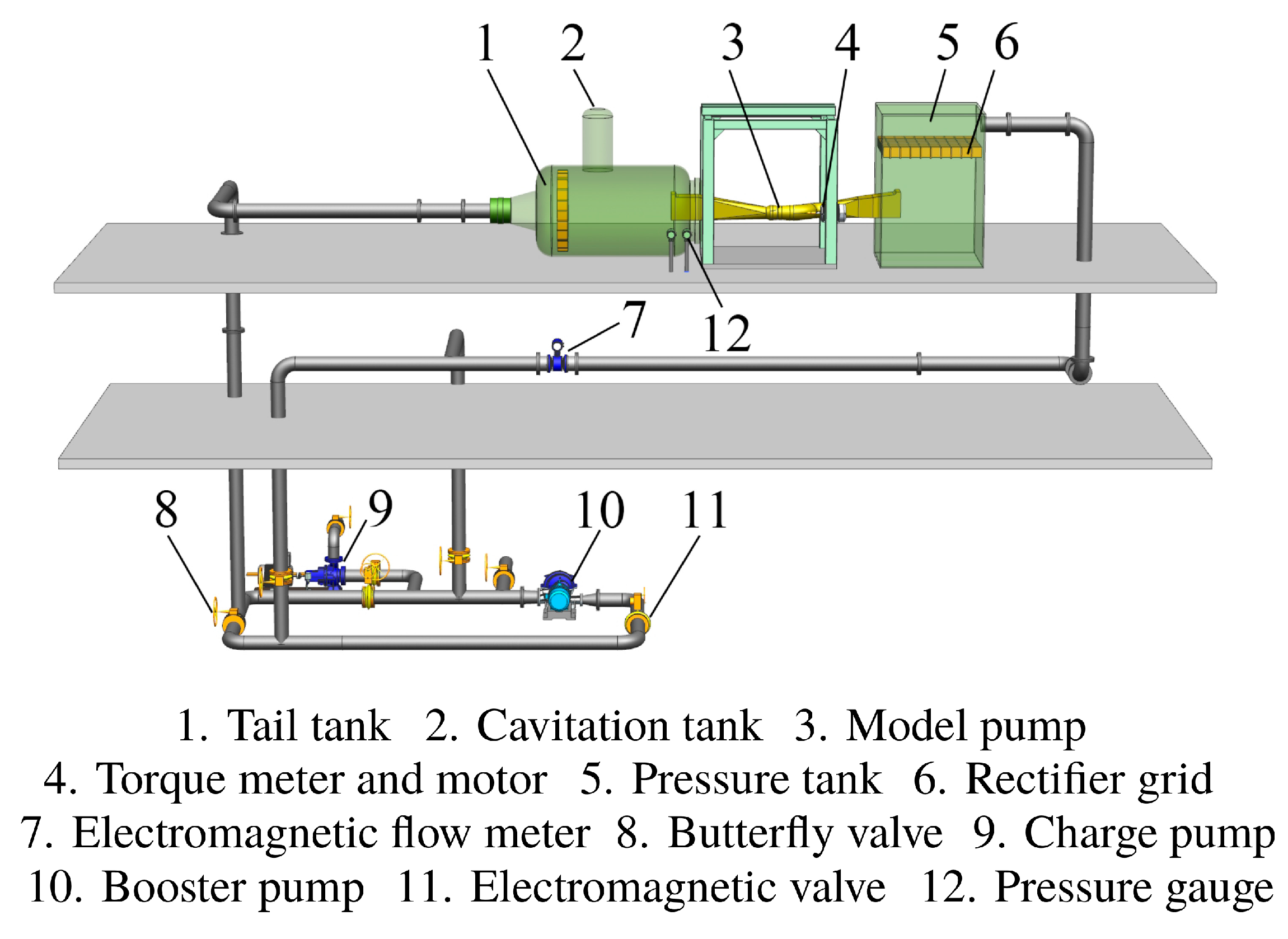
2.3. Experimental Setup
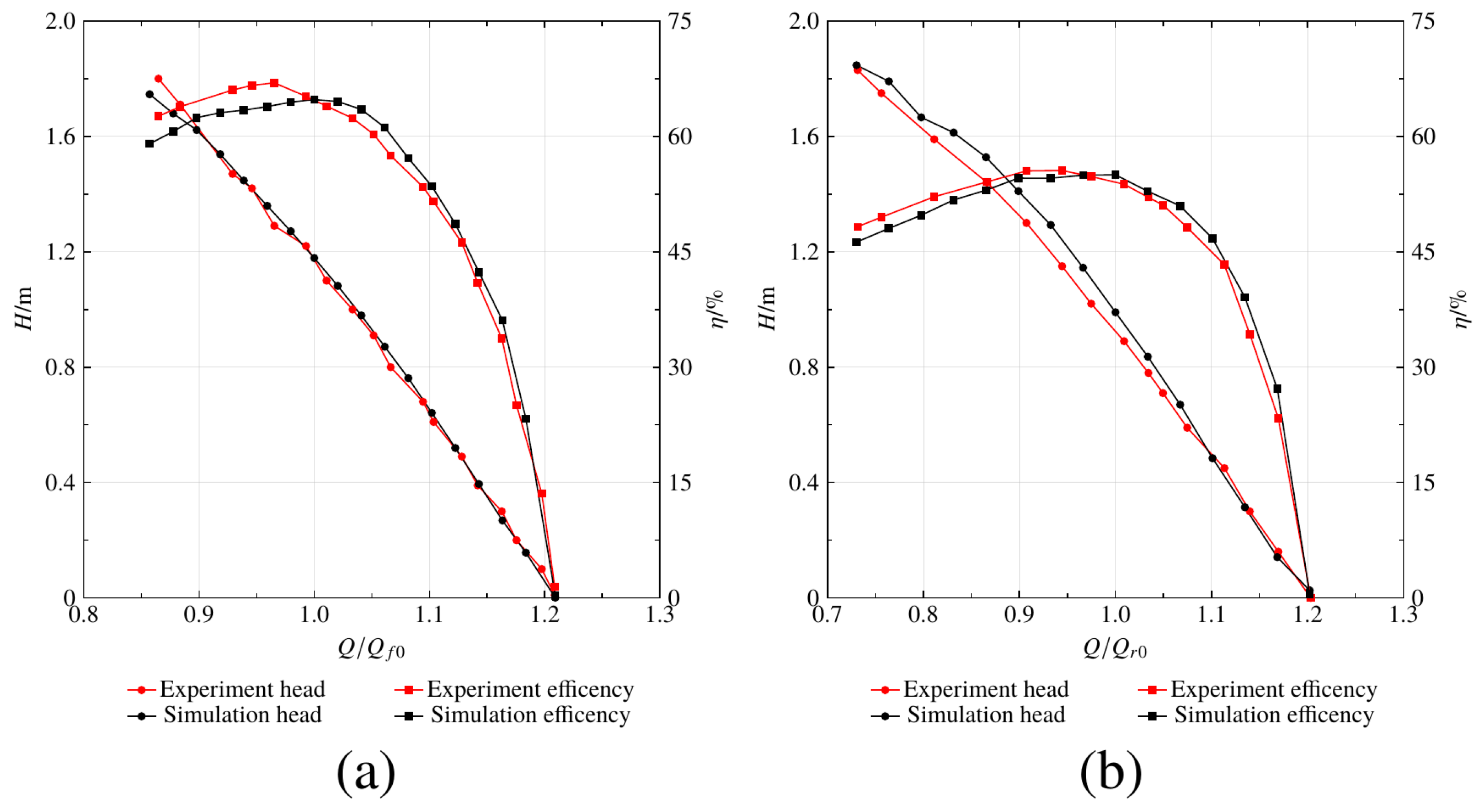
2.4. Validation
3. Results and Discussion
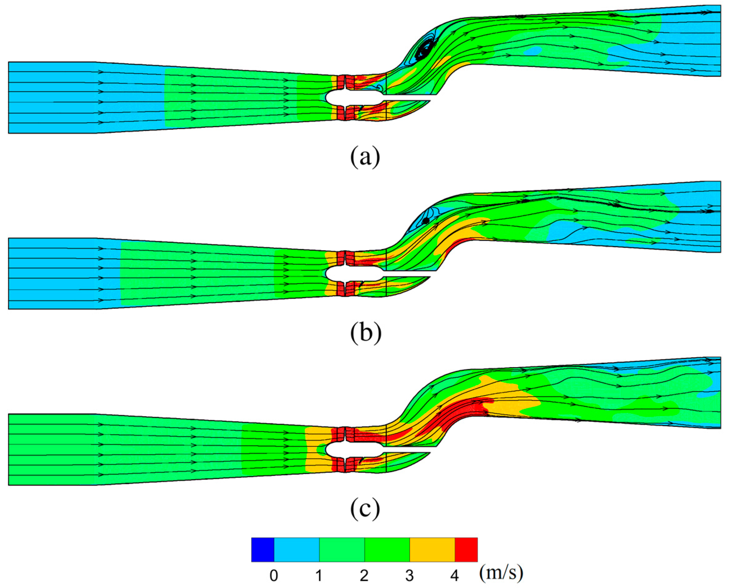
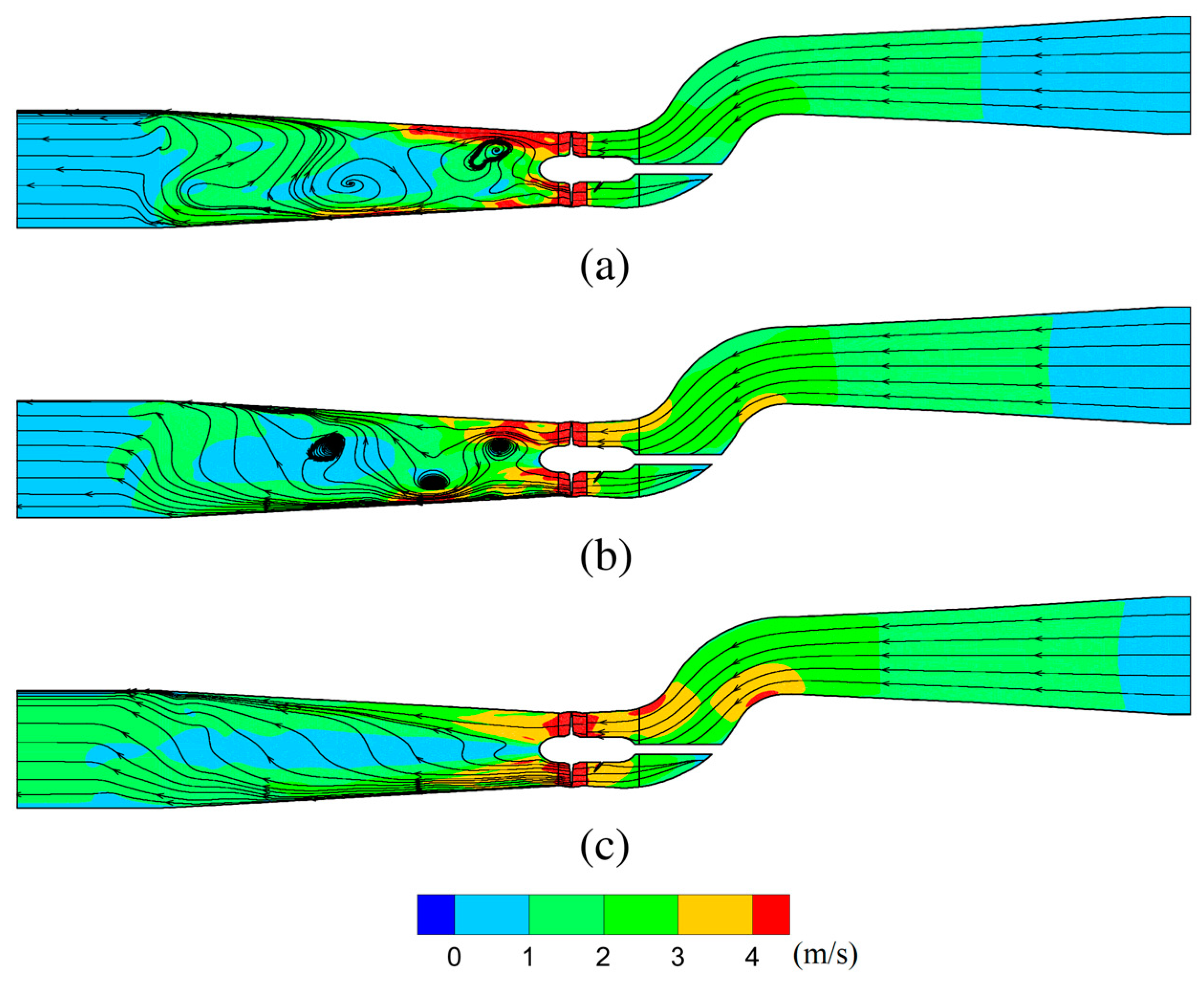
3.1. Flow Field in the Entire Domain
3.2. Flow Field Inside the Impeller and Guide Vane
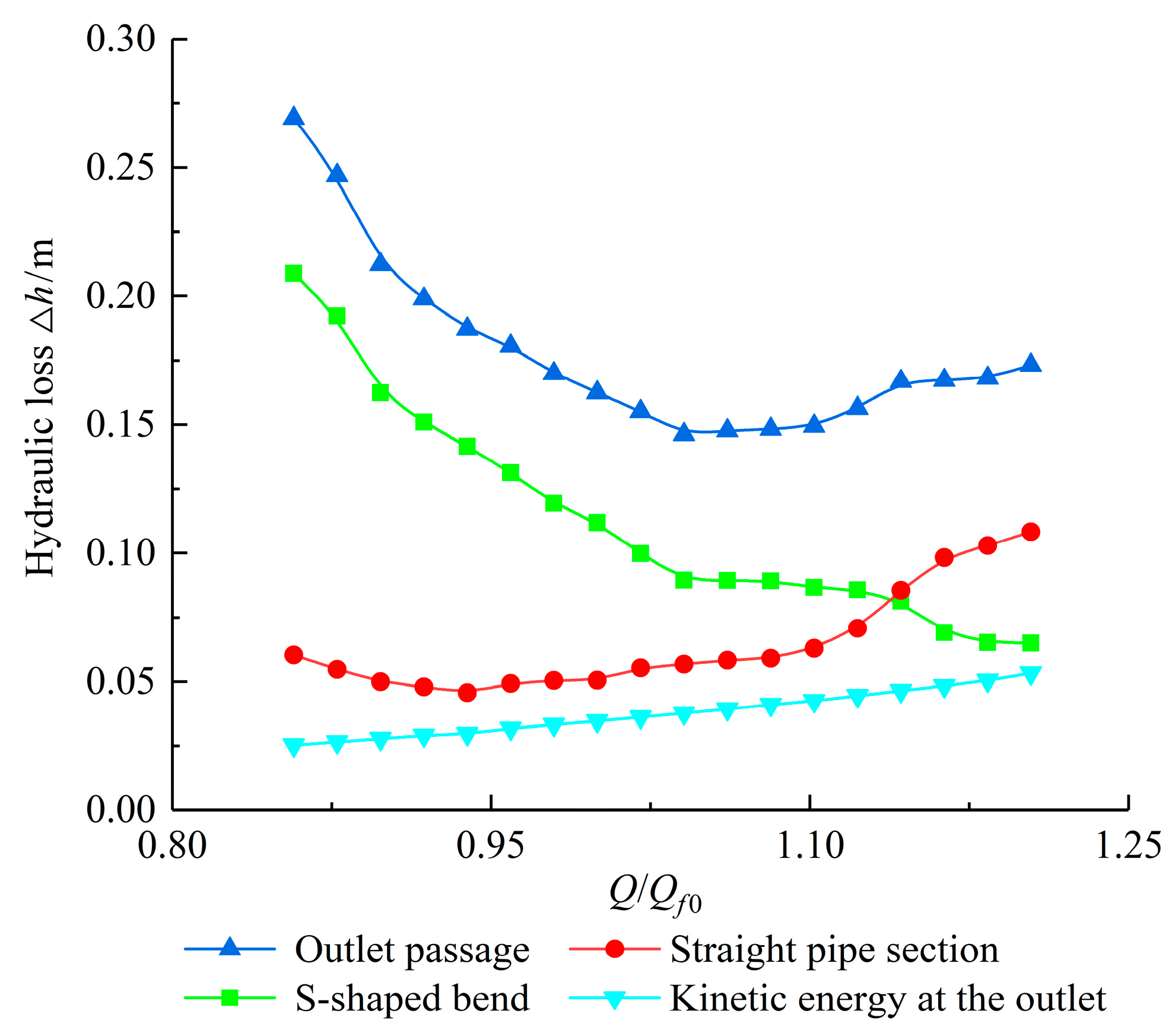
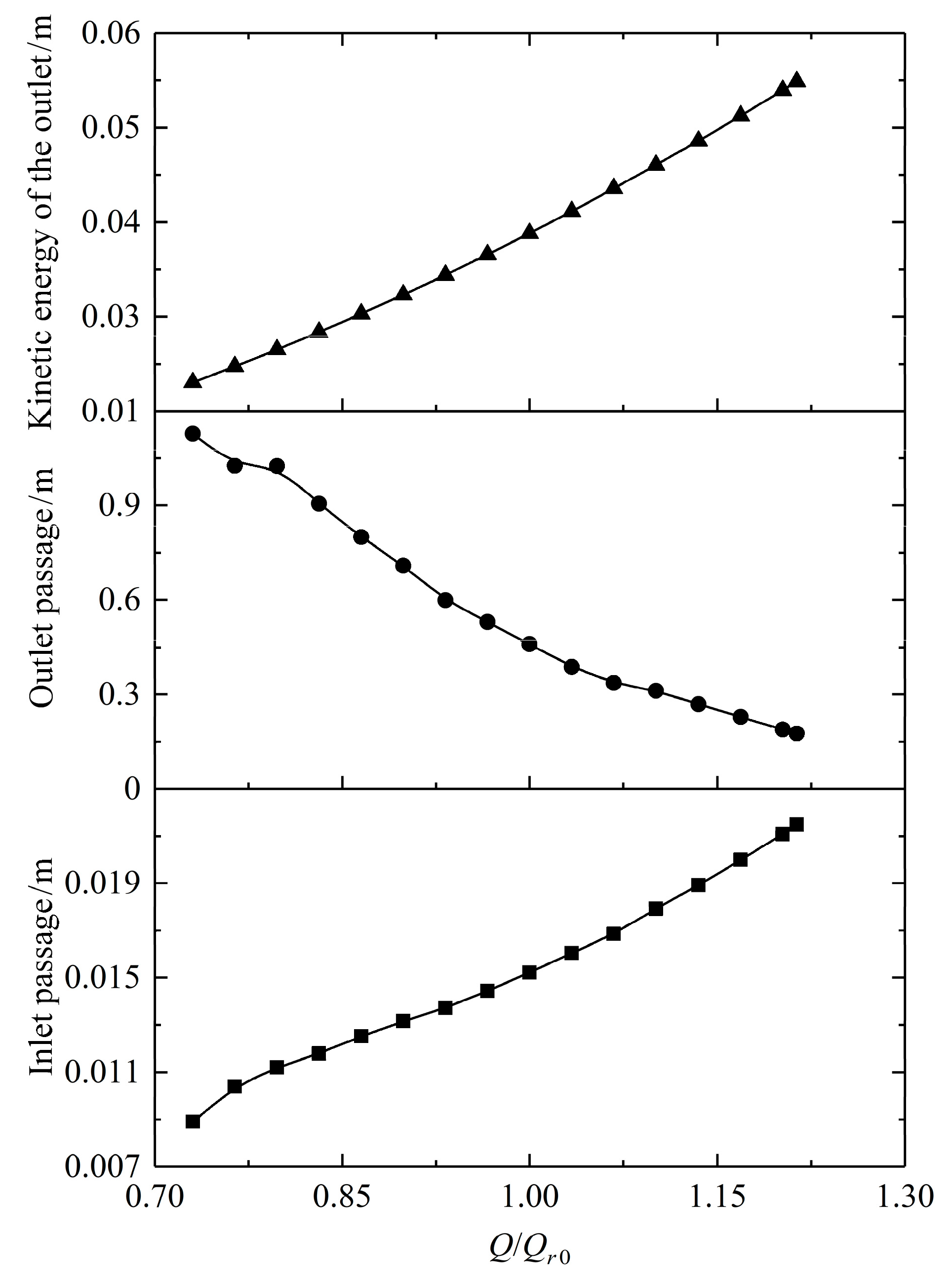
3.3. Hydraulic Loss of Flow Passages
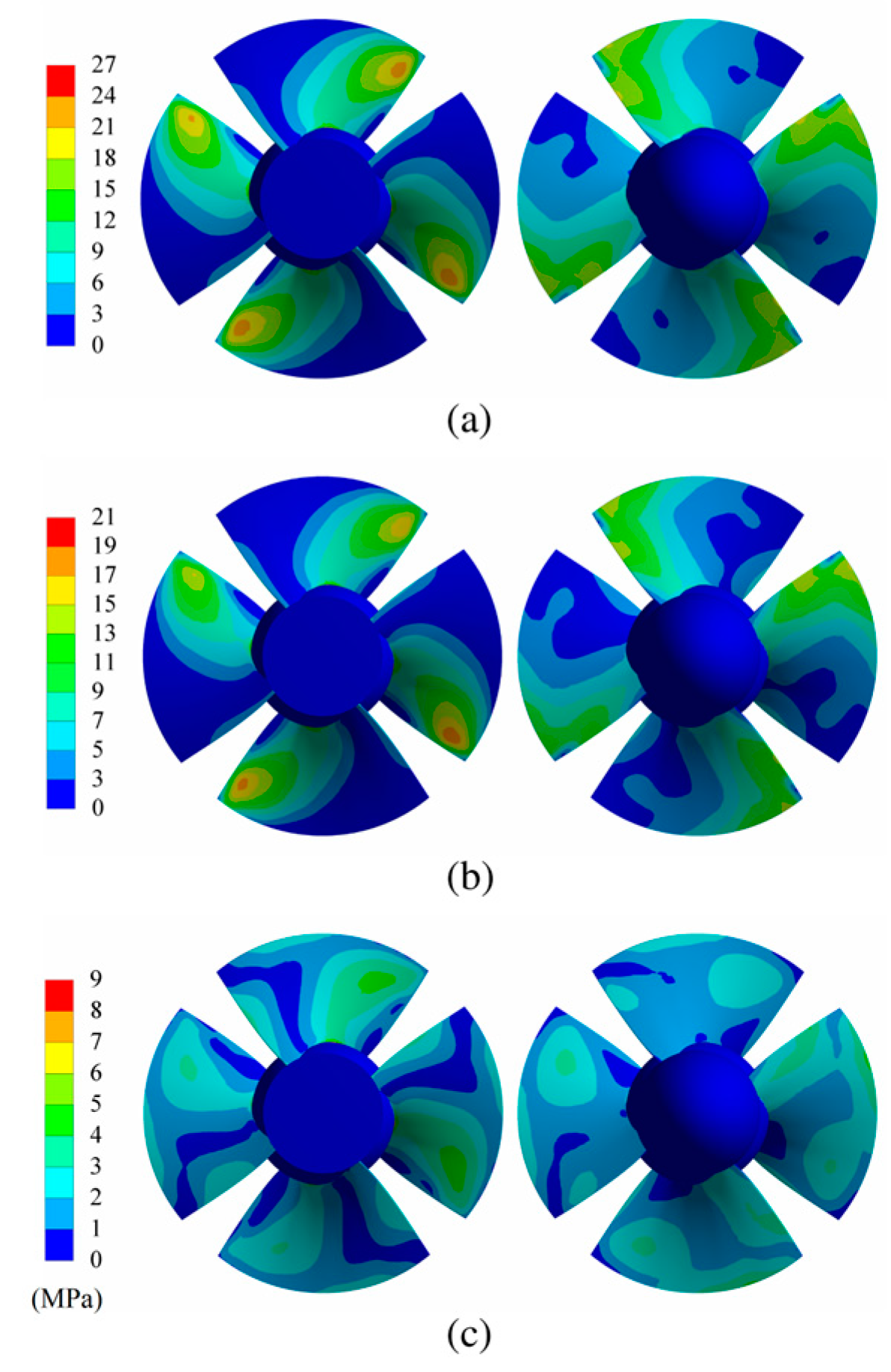
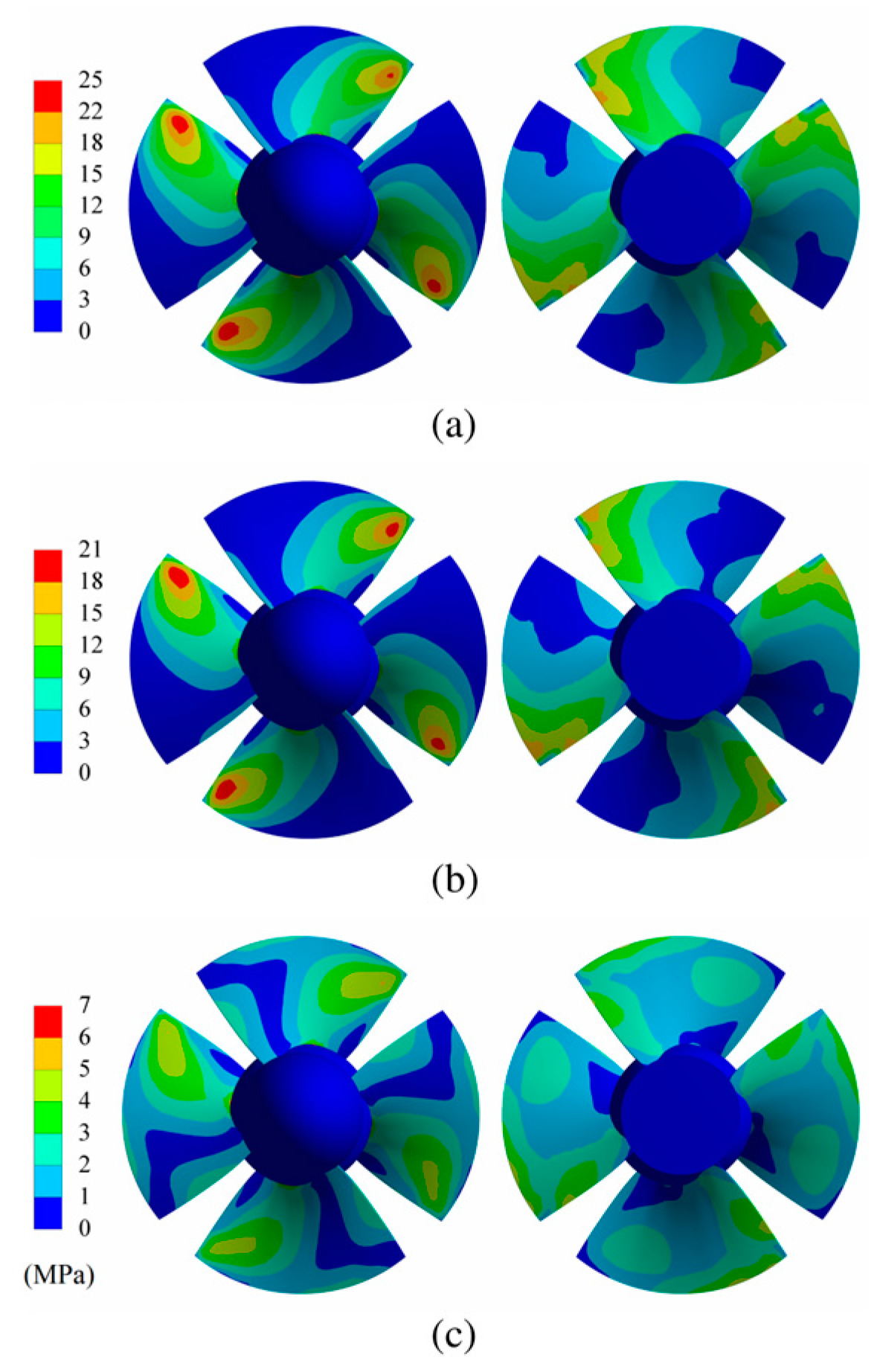
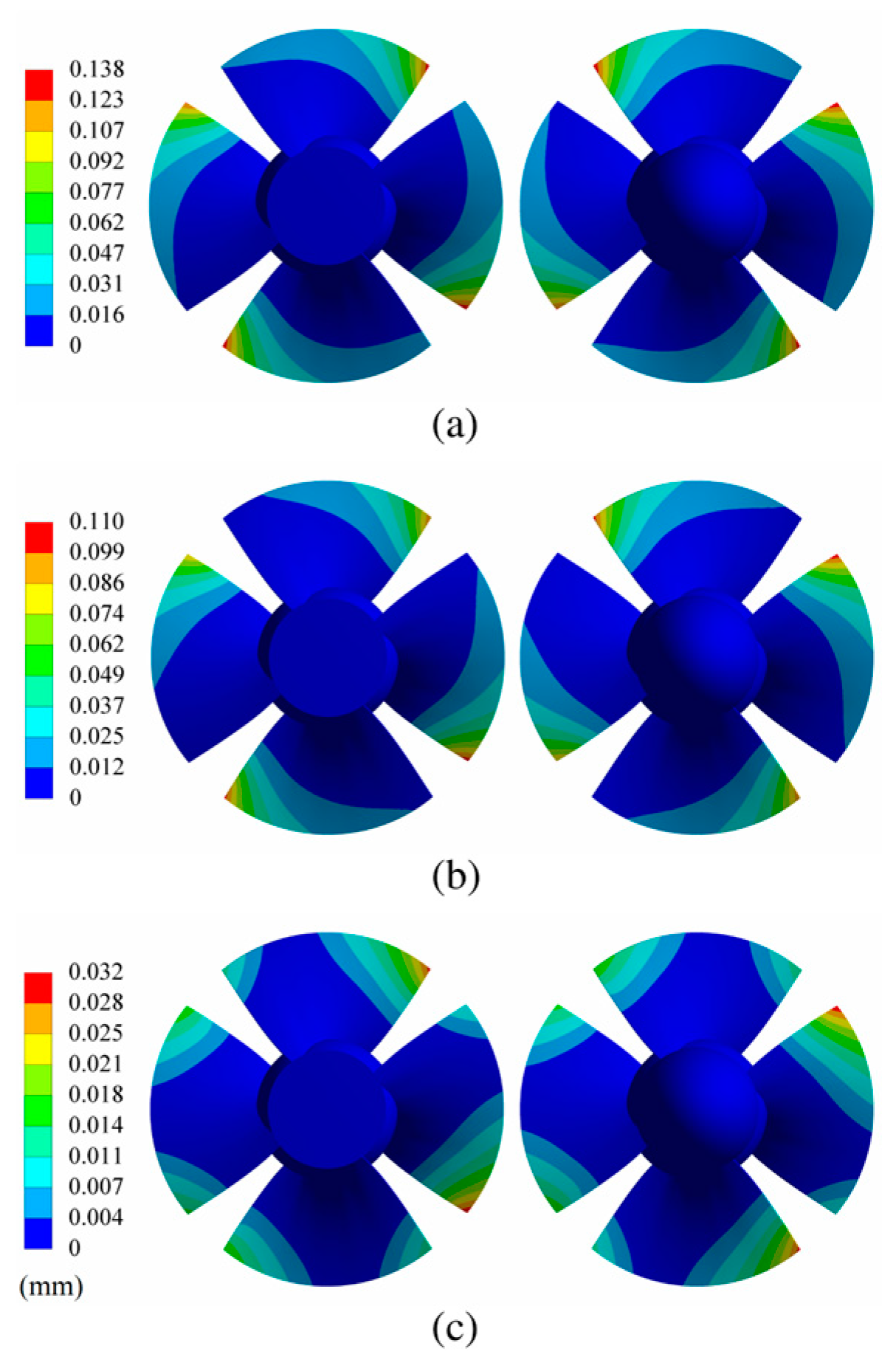
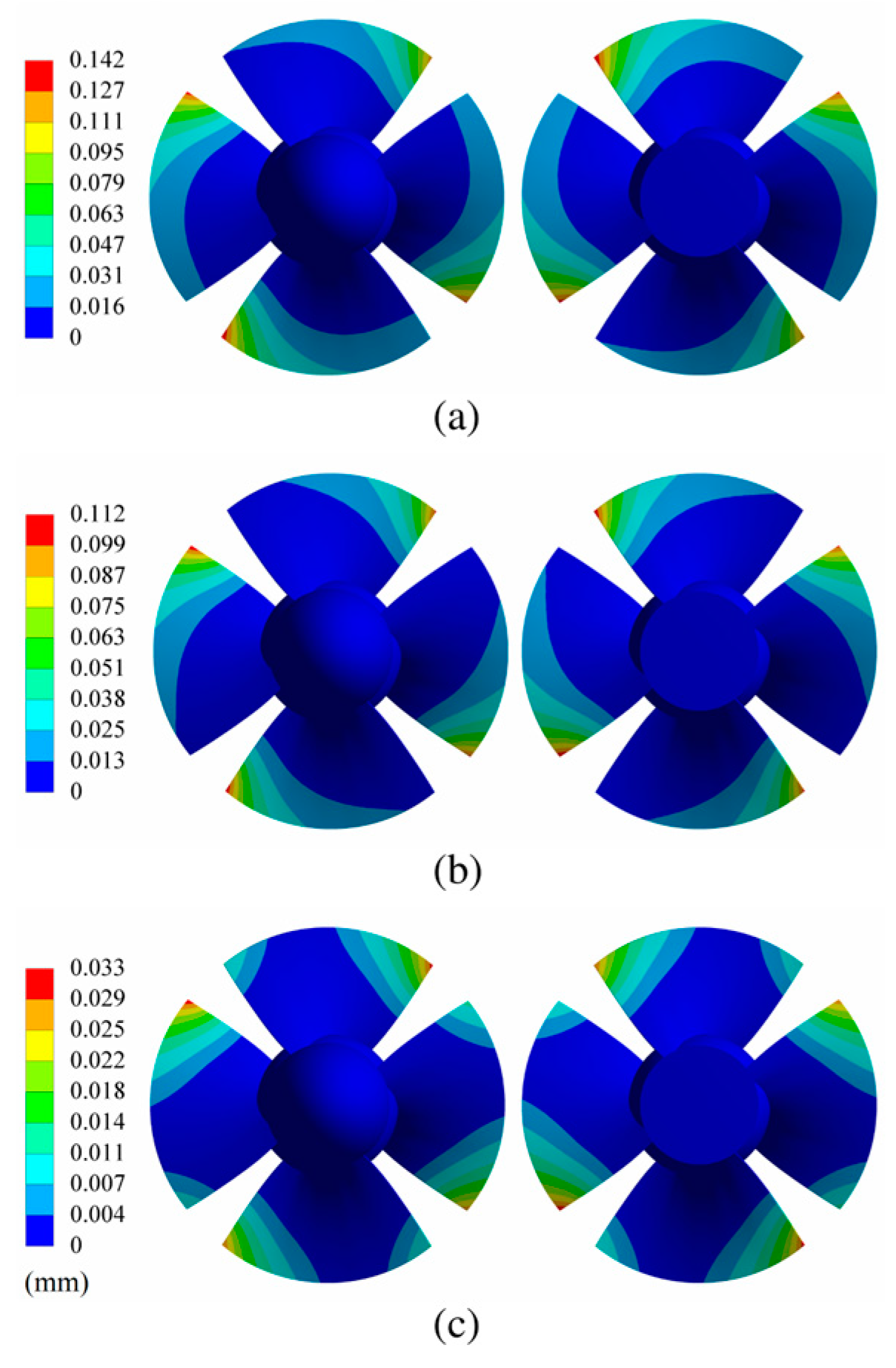
3.4. FSI
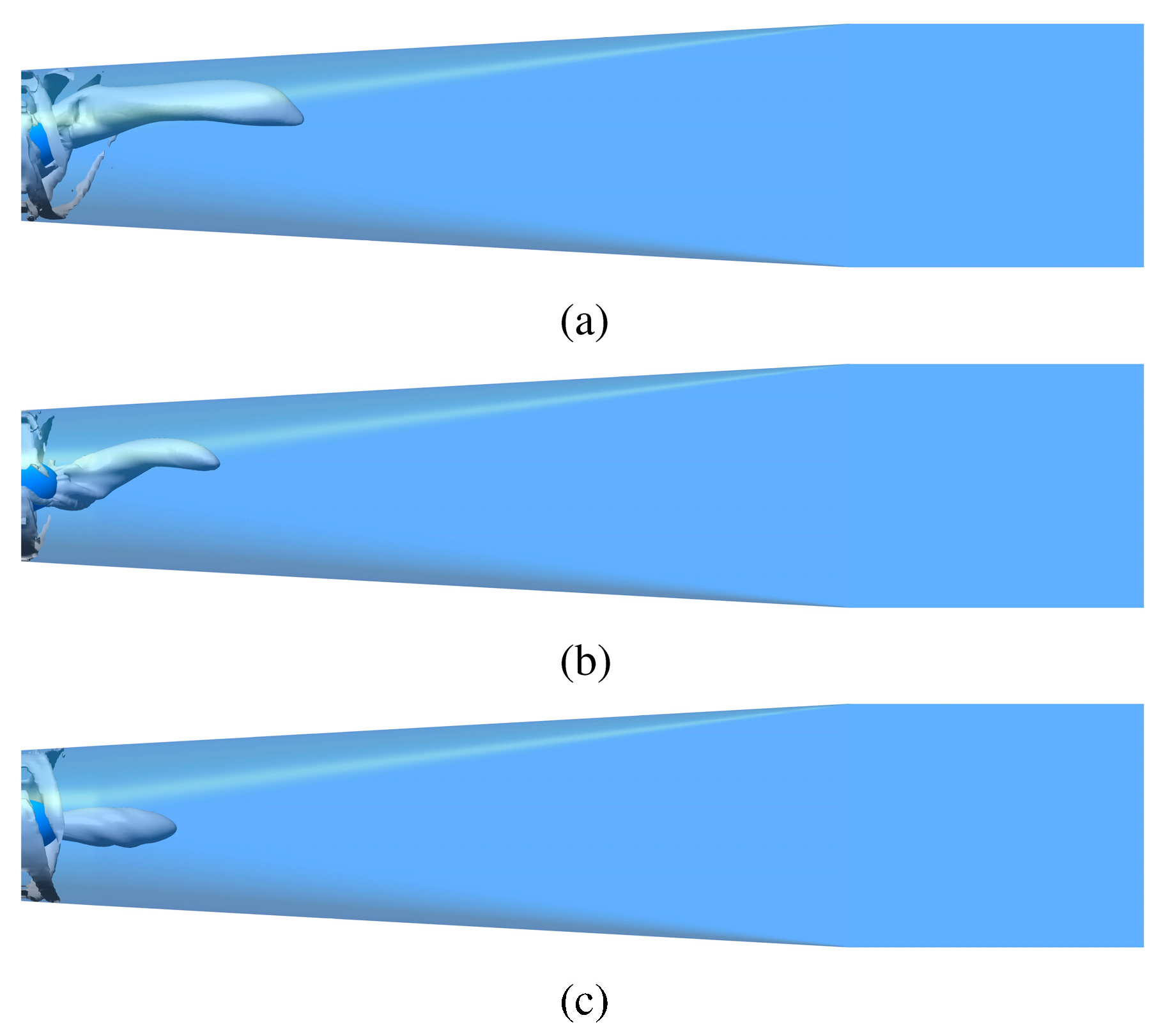
3.5. Cavitation
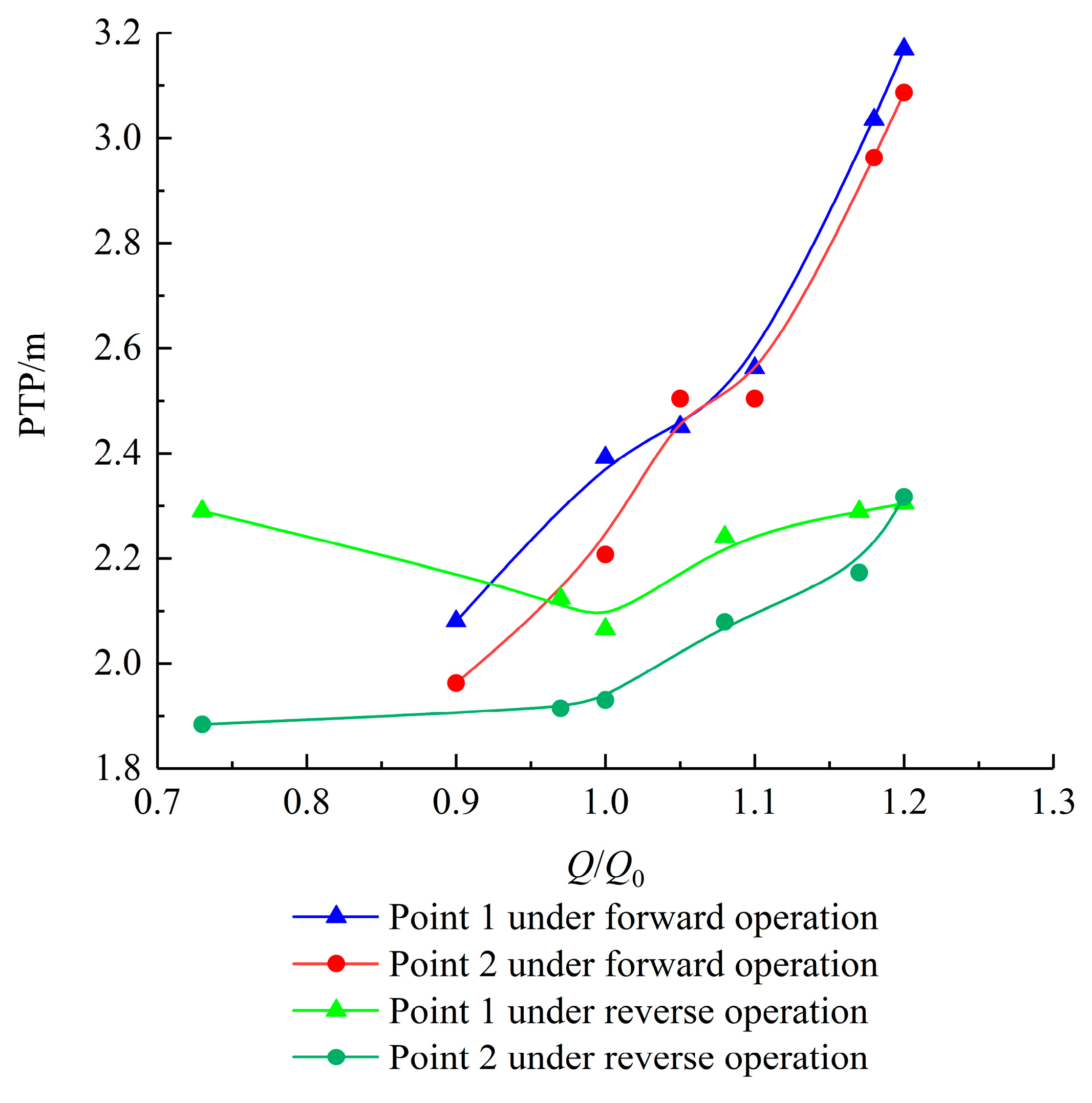
3.6. Pressure Fluctuation
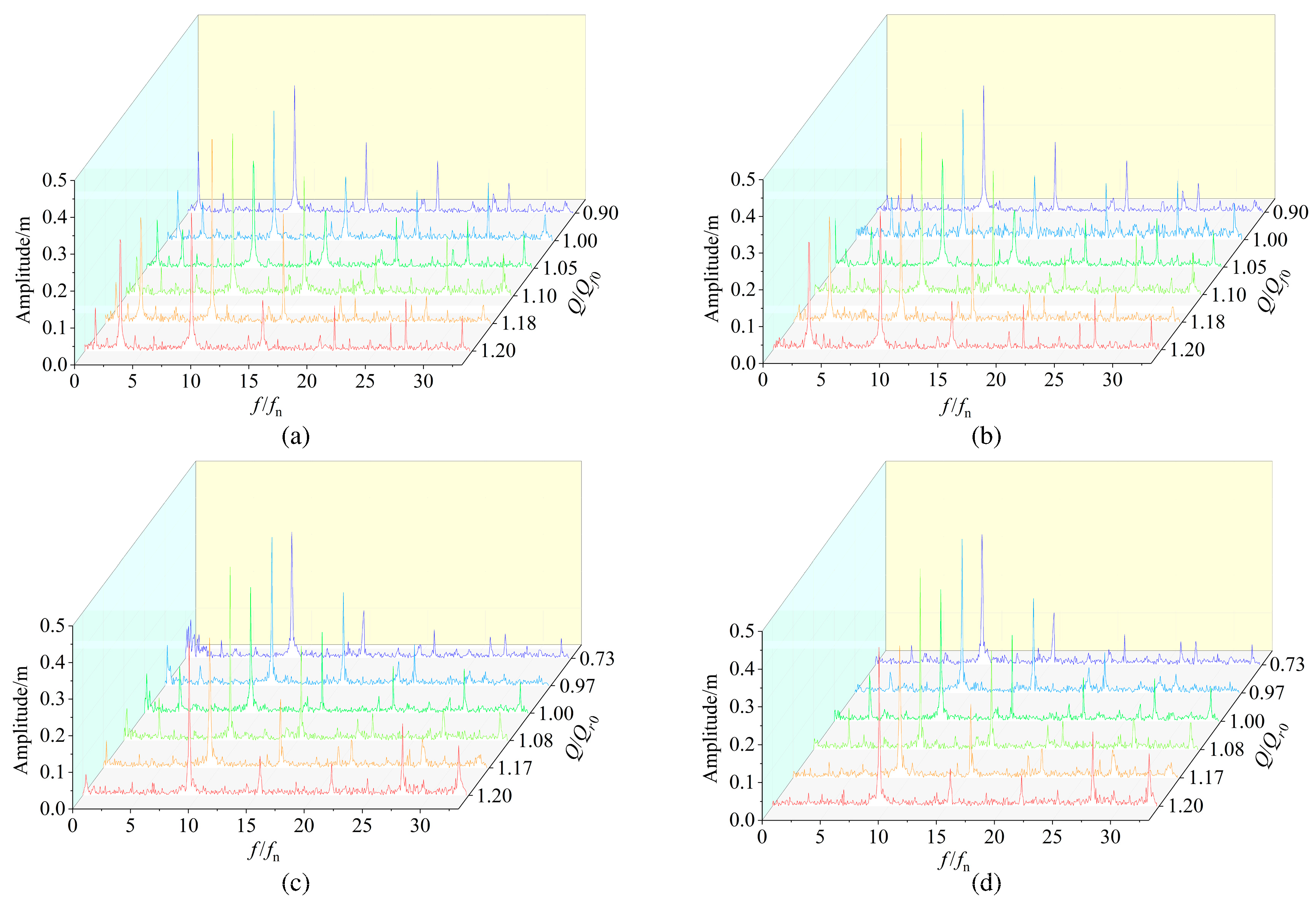
3.7. Vibration
4. Conclusions
Author Contributions
Funding
Data Availability Statement
Conflicts of Interest
References
- Liu, C. Pumps and Pumping Stations; China Water & Power Press: Beijing, China, 2003. [Google Scholar]
- Goltz, I.; Kosyna, G.; Stark, U.; Saathoff, H.; Bross, S. Stall inception phenomena in a single-stage axial-flow pump. Proc. Inst. Mech. Eng. Part A J. Power Energy 2003, 217, 471–479. [Google Scholar] [CrossRef]
- Li, Y.; Wang, F. Numerical investigation of performance of an axial-flow pump with inducer. J. Hydrodyn. 2007, 19, 705–711. [Google Scholar] [CrossRef]
- Zhang, D.; Shi, W.; Bin, C.; Guan, X. Unsteady flow analysis and experimental investigation of axial-flow pump. J. Hydrodyn. Ser B 2010, 22, 35–43. [Google Scholar] [CrossRef]
- Prasad, V. Numerical simulation for flow characteristics of axial flow hydraulic turbine runner. Energy Procedia 2012, 14, 2060–2065. [Google Scholar] [CrossRef]
- Kan, K.; Zheng, Y.; Chen, Y.; Xie, Z.; Yang, G.; Yang, C. Numerical study on the internal flow characteristics of an axial-flow pump under stall conditions. J. Mech. Sci. Technol. 2018, 32, 4683–4695. [Google Scholar] [CrossRef]
- Yang, F.; Lin, Z.; Li, J.; Nasr, A.; Cong, W.; Li, C. Analysis of internal flow characteristics and structure optimization of vertical submersible axial flow pump device. Adv. Mech. Eng. 2022, 14, 1–23. [Google Scholar] [CrossRef]
- Pozarlik, A.K.; Kok, J.B.W. Numerical investigation of one-and two-way fluid-structure interaction in combustion systems. In Proceedings of the International Conference on Computational Methods for Coupled Problems in Science and Engineering, Ibiza, Spain, 21 May–23 May 2007. [Google Scholar]
- Benra, F.K.; Dohmen, H.J.; Pei, J.; Schuster, S.; Wan, B. A comparison of one-way and two-way coupling methods for numerical analysis of fluid-structure interactions. J. Appl. Math. 2011, 2011, 853560. [Google Scholar] [CrossRef]
- Lerche, A.H.; Moore, J.J.; White, N.M.; Hardin, J. Dynamic stress prediction in centrifugal compressor blades using fluid structure interaction. Turbo Expo Power Land Sea Air 2012, 44724, 191–200. [Google Scholar]
- Birajdar, R.; Keste, A. Prediction of flow-induced vibrations due to impeller hydraulic unbalance in vertical turbine pumps using one-way fluid- structure interaction. J. Vib. Eng. Technol. 2020, 8, 417–430. [Google Scholar] [CrossRef]
- Shi, L.; Zhu, J.; Wang, L. Analysis of Strength and Modal Characteristics of a Full Tubular Pump Impeller Based on Fluid-Structure Interaction. Res. Sq. 2021. [Google Scholar] [CrossRef]
- Zhang, D.; Shi, W.; Van Esch BP, M.B.; Shi, L.; Dubuisson, M. Numerical and experimental investigation of tip leakage vortex trajectory and dynamics in an axial flow pump. Comput. Fluids 2015, 112, 61–71. [Google Scholar] [CrossRef]
- Zhang, D.; Shi, W.; Pan, D.; Dubuisson, M. Numerical and experimental investigation of tip leakage vortex cavitation patterns and mechanisms in an axial flow pump. J. Fluids Eng. 2015, 137, 121103. [Google Scholar] [CrossRef]
- Feng, H.; Wan, Y.; Fan, Z. Numerical investigation of turbulent cavitating flow in an axial flow pump using a new transport-based model. J. Mech. Sci. Technol. 2020, 34, 745–756. [Google Scholar] [CrossRef]
- Wang, C.; Wu, S.; Shi, W.; Yao, J. Numerical calculation and experimental research of pressure fluctuation in the pump under different operating conditions. J. Vibroeng. 2013, 15, 2049–2056. [Google Scholar]
- Ma, P.; Wang, J.; Li, H. Numerical analysis of pressure pulsation for a bidirectional pump under positive and reverse operation. Adv. Mech. Eng. 2014, 6, 730280. [Google Scholar] [CrossRef]
- Xie, C.; Tang, F.; Zhang, R.; Zhou, W.; Zhang, W.; Yang, F. Numerical calculation of axial-flow pump’s pressure fluctuation and model test analysis. Adv. Mech. Eng. 2018, 10, 1687814018769775. [Google Scholar] [CrossRef]
- Shervani-Tabar, M.T.; Ettefagh, M.M.; Lotfan, S.; Safarzadeh, H. Cavitation intensity monitoring in an axial flow pump based on vibration signals using multi-class support vector machine. Proc. Inst. Mech. Eng. Part C J. Mech. Eng. Sci. 2018, 232, 3013–3026. [Google Scholar] [CrossRef]
- Menter, F.R. Review of the shear-stress transport turbulence model experience from an industrial perspective. J. Comput. Fluid Dyn. 2009, 23, 305–316. [Google Scholar] [CrossRef]
- Feng, W.; Cheng, Q.; Guo, Z.; Qian, Z. Simulation of cavitation performance of an axial flow pump with inlet guide vanes. Adv. Mech. Eng. 2016, 8, 1687814016651583. [Google Scholar] [CrossRef]
- Shi, W.; Wang, C.; Wang, W.; Pei, B. Numerical calculation on cavitation pressure pulsation in centrifugal pump. Adv. Mech. Eng. 2014, 6, 367631. [Google Scholar] [CrossRef]
- Marsh, P.; Ranmuthugala, D.; Penesis, I.; Thomas, G. Numerical investigation of the influence of blade helicity on the performance characteristics of vertical axis tidal turbines. Renew. Energy 2015, 81, 926–935. [Google Scholar] [CrossRef]
- Tan, L.; Zhu, B.; Wang, Y.; Shuliang, C.; Gui, S. Numerical study on characteristics of unsteady flow in a centrifugal pump volute at partial load condition. Eng. Comput. 2015, 32, 1549–1566. [Google Scholar] [CrossRef]
- Zheng, Y.; Li, P.; Chen, X.; Wang, C. Hydraulic design on circulation pipe system for hydraulic machinery multifunctional model test bench. Fluid Mach. 2001, 29, 16–18. [Google Scholar]
- Lu, L. Optimized Hydraulic Design of High Performance Large Low Head Pump Units; China Water & Power Press: Beijing, China, 2013; Volume 91. [Google Scholar]
- Zhang, R.; Chen, H. Numerical Simulation and Flow Diagnosis of Axial-Flow Pump at Part-Load Condition; De Gruyter: Berlin, Germany, 2012; Volume 29, pp. 1–7. [Google Scholar]
- Zhang, D.; Geng, L.; Shi, W. Experimental investigation on pressure fluctuation and vibration in axial-flow pump model. Nongye Jixie Xuebao/Trans. Chin. Soc. Agric. Mach. 2015, 46, 66–72. [Google Scholar]


| Nodes | Elements | Maximum Stress (MPa) |
|---|---|---|
| 1,328,790 | 408,440 | 21.314 |
| 799,963 | 251,839 | 20.947 |
| 447,851 | 144,995 | 20.118 |
| 316,158 | 107,761 | 18.837 |
| 247,435 | 83,375 | 17.364 |
| Direction | Q/Q0 | X Direction | Y Direction | Z Direction | |||
|---|---|---|---|---|---|---|---|
| PTP Values | PF | PTP Values | PF | PTP Values | PF | ||
| Forward operation | 1.20 | 0.742 | 3 | 0.732 | 3 | 1.665 | 3 |
| 1.16 | 0.757 | 15 | 0.566 | 3 | 1.514 | 15 | |
| 1.10 | 0.723 | 9 | 0.625 | 4 | 1.870 | 4 | |
| 0.90 | 0.796 | 3 | 0.830 | 3 | 1.963 | 3 | |
| Reverse operation | 1.20 | 0.645 | 3 | 0.615 | 3 | 1.533 | 3 |
| 1.05 | 0.474 | 3 | 0.513 | 3 | 1.230 | 4 | |
| 0.97 | 0.547 | 3 | 0.581 | 4 | 1.475 | 1 | |
| 0.73 | 0.947 | 1 | 1.104 | 1 | 2.891 | / | |
Disclaimer/Publisher’s Note: The statements, opinions and data contained in all publications are solely those of the individual author(s) and contributor(s) and not of MDPI and/or the editor(s). MDPI and/or the editor(s) disclaim responsibility for any injury to people or property resulting from any ideas, methods, instructions or products referred to in the content. |
© 2025 by the authors. Licensee MDPI, Basel, Switzerland. This article is an open access article distributed under the terms and conditions of the Creative Commons Attribution (CC BY) license (https://creativecommons.org/licenses/by/4.0/).
Share and Cite
Zhang, F.; Zheng, Y.; Li, G.; Dai, J. Numerical and Experimental Investigation of the Ultra-Low Head Bidirectional Shaft Extension Pump Under Near-Zero Head Conditions. Machines 2025, 13, 220. https://doi.org/10.3390/machines13030220
Zhang F, Zheng Y, Li G, Dai J. Numerical and Experimental Investigation of the Ultra-Low Head Bidirectional Shaft Extension Pump Under Near-Zero Head Conditions. Machines. 2025; 13(3):220. https://doi.org/10.3390/machines13030220
Chicago/Turabian StyleZhang, Fulin, Yuan Zheng, Gaohui Li, and Jing Dai. 2025. "Numerical and Experimental Investigation of the Ultra-Low Head Bidirectional Shaft Extension Pump Under Near-Zero Head Conditions" Machines 13, no. 3: 220. https://doi.org/10.3390/machines13030220
APA StyleZhang, F., Zheng, Y., Li, G., & Dai, J. (2025). Numerical and Experimental Investigation of the Ultra-Low Head Bidirectional Shaft Extension Pump Under Near-Zero Head Conditions. Machines, 13(3), 220. https://doi.org/10.3390/machines13030220