Method of Dynamic Modeling and Robust Optimization for Chain Transmission Mechanism with Time-Varying Load Uncertainty

Abstract

Time-varying driving loads and uncertain structural parameters affect the transmission accuracy of chain transmission mechanisms. To enhance the transmission accuracy and placement consistency of these mechanisms, a robust optimization design method based on Karhunen–Loeve expansion and Polynomial Chaos Expansion (KL-PCE) is proposed. First, a dynamic model of the chain transmission mechanism, considering multiple contact modes, is established, and the model’s accuracy is verified through experiments. Then, based on the KL-PCE method, a mapping relationship between uncertain input parameters and output responses is established. A robust optimization design model for the chain transmission process is formulated, with transmission accuracy and consistency as objectives. Finally, case studies are used to verify the effectiveness of the proposed method. Thus, the transmission accuracy of the chain transmission mechanism is improved, providing a theoretical foundation for the design of chain transmission mechanisms under time-varying load uncertainties and for improving the accuracy of other complex mechanisms.

1. Introduction

Chain transmission mechanisms are widely used in mechanical structures, such as machine tools, special equipment, industrial machinery, agricultural machinery, construction machinery, aerospace, and medical devices. They offer high reliability and efficient transmission, with strong adaptability to heavy loads and harsh environments. However, due to random uncertainties in structural, physical, and drive parameters, the delivery precision and positional consistency of the transmitted objects are affected during operation. To enhance the robustness of chain transmission mechanisms during the design phase, robust optimization design methods can reduce the sensitivity of the mechanism’s movement to random uncertainties while ensuring motion accuracy.

In previous studies, researchers have conducted a series of investigations on chain drive mechanisms. Li et al. [1] proposed a feasible solution for the robust optimization of multi-gap chain transmission mechanisms by using a data-driven modeling framework based on deep neural networks, but without considering the influence of time-varying loads. Zhuang et al. [2] optimized the design of mechanical chain drives using wireless sensor network data algorithms, thereby improving the reliability and stability of scraper conveyors, and providing a theoretical reference for the robust optimization of chain transmission mechanisms. Chai et al. [3] introduced a new method based on multi-disciplinary design optimization, and then established system optimization objectives and subsystems to obtain the kinematic principles and optimal parameter values of chain drives, without considering the effect of parameter uncertainty. To analyze the operational stability of chain transmission scraper conveyors, Jiang et al. [4] established a combined simulation model for the chain transmission mechanism, analyzing the system’s dynamic characteristics and failure causes. In order to reduce the polygonal effect in chain transmission mechanisms, Hong et al. [5] proposed a compensation method to optimize the design of the chain transmission mechanism, thereby effectively improving the transmission performance of the chain transmission system. To enhance the control and guiding capabilities of the in-wheel motor steering transmission mechanical chain transmission and improve the transmission efficiency of the in-wheel engine steering mechanical chain transmission, Da et al. [6] proposed a control method for an in-wheel motor-guided transmission mechanical chain gearbox, thereby enhancing the robustness and adaptability of the hub motor steering transmission mechanical chain transmission. To analyze the noise characteristics and structural design of chain transmission systems under complex working conditions, such as high-speed and overload, Cheng et al. [7] studied the system design and noise characteristics of a new dual-clutch automatic transmission with a double-tooth chain, achieving structural optimization design.

It can be seen that the above references have conducted research on the parameter optimization design of chain transmission mechanisms, which can provide a solid foundation for the robust optimization of chain transmission mechanisms. There has been relatively little research on the robust optimization design of chain transmission mechanisms. However, in other engineering fields, relevant research on robust optimization design has been conducted, which can provide references for the robust design of chain transmission mechanisms. Addressing the problem of improving the aerodynamic performance of drone wings and bodies, Wang et al. [8] used the Gradient-Enhanced Polynomial Chaos Expansion (GPCE) method to construct statistical moments related to the mean and variance, and established a gradient-based robust optimization design model, validating its effectiveness. To avoid the curse of dimensionality in the robust optimization design process, Zhang et al. [9] combined the polynomial chaos expansion method and proposed a technique called R-Opt, a robust aerodynamic optimization method that improved average aerodynamic performance and reduced the standard deviation of the objective. Najlawi et al. [10] developed a combined multi-objective imperialist competitive algorithm and Monte Carlo method for the multi-objective robust optimization design of sewing machine needle rods and take-up rods (NBTTL), significantly reducing the sensitivity of the mechanism’s performance to design parameters. For the challenges of strong non-linearity and long experimental and simulation prediction times in the ammunition loading mechanism, Zhang et al. [11] proposed a data-driven modeling method based on artificial neural networks, and performed a robust optimization design for the ammunition loading process using the data-driven model. In robot mechanism research, current robust optimization studies mainly focus on planar closed-loop or open-chain mechanisms [12,13]. For example, Wu and Rao [14] proposed a tolerance allocation optimization technique through interval uncertainty analysis, which effectively saves manufacturing costs while ensuring positioning accuracy. Du et al. [15] proposed a planar mechanism robust optimization method based on dual-loop Monte Carlo simulation, improving the robustness of motion accuracy. To solve the general design problems of complex engineering systems, several uncertainty optimization methods have been developed [16,17,18,19]. For instance, Lee [20] and others introduced the so-called point estimation method in robust optimization to improve structural efficiency. Chatterjee [21] and others proposed a universal robust design framework integrating surrogate modeling techniques to address complex and highly non-linear problems. Lee and Rahman [22] proposed a new robust optimization method based on polynomial chaos expansion, considering the correlation of uncertain variables. Zafar et al. [23] considered the time-varying reliability of systems and proposed a dynamic robust optimization method. Jiang et al. [24] combined parallel efficient global optimization with adaptive Kriging techniques, introducing time-varying uncertainty in robust optimization. Cheng et al. [25] proposed a robust balancing optimization method, improving the robustness of structural dynamic characteristics by introducing the overlap coefficient between the interval boundary angles. These general uncertainty optimization techniques provide algorithmic insights for the robust optimization of chain transmission mechanisms.

In summary, previous studies have shown relatively little research on the robust design of chain transmission mechanisms considering time-varying load uncertainties. Therefore, in order to achieve a robust design of chain transmission mechanisms considering time-varying load uncertainties, this paper proposes a robust optimization design method for chain transmission mechanisms based on K-L expansion and PCE. The main contributions and innovations are as follows:

(1)

A dynamic model of the chain transmission mechanism considering multiple clearances was established, and the accuracy of the simulation model was verified through experiments.

(2)

A robust optimization design method for the chain transmission mechanism based on K-L expansion and PCE was proposed. First, the K-L expansion method was used for the dimensionality reduction of the random driving loads. Then, based on the PCE method, a fast uncertainty propagation analysis of the chain transmission mechanism was conducted, and a robust optimization design model for the chain transmission mechanism was established.

(3)

The effectiveness of the proposed method was verified through engineering examples, providing theoretical reference for the robust optimization design of complex engineering chain transmission problems.

The structure of this paper is as follows. Section 2 presents the dynamic modeling and experimental validation of the chain transmission mechanism. Section 3 discusses the robust optimization design of the chain transmission mechanism considering random loads. Section 4 provides a case study analysis, and Section 5 presents the conclusions.

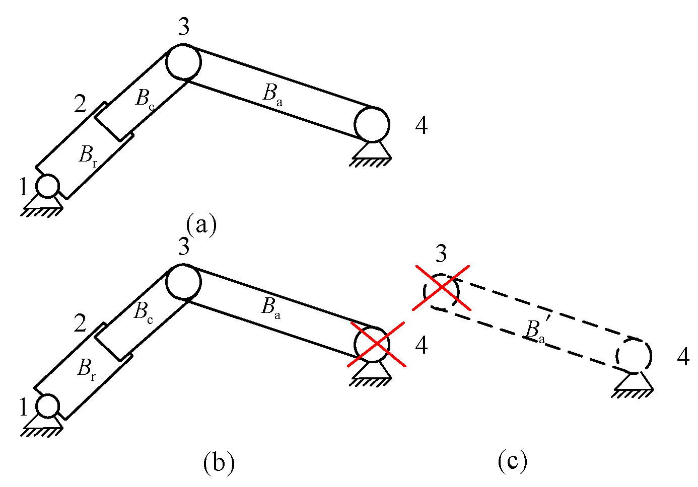
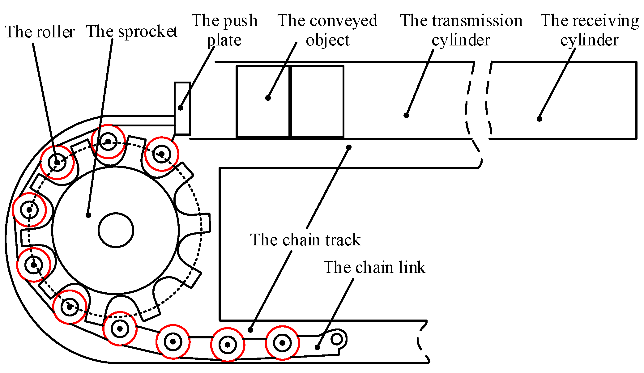
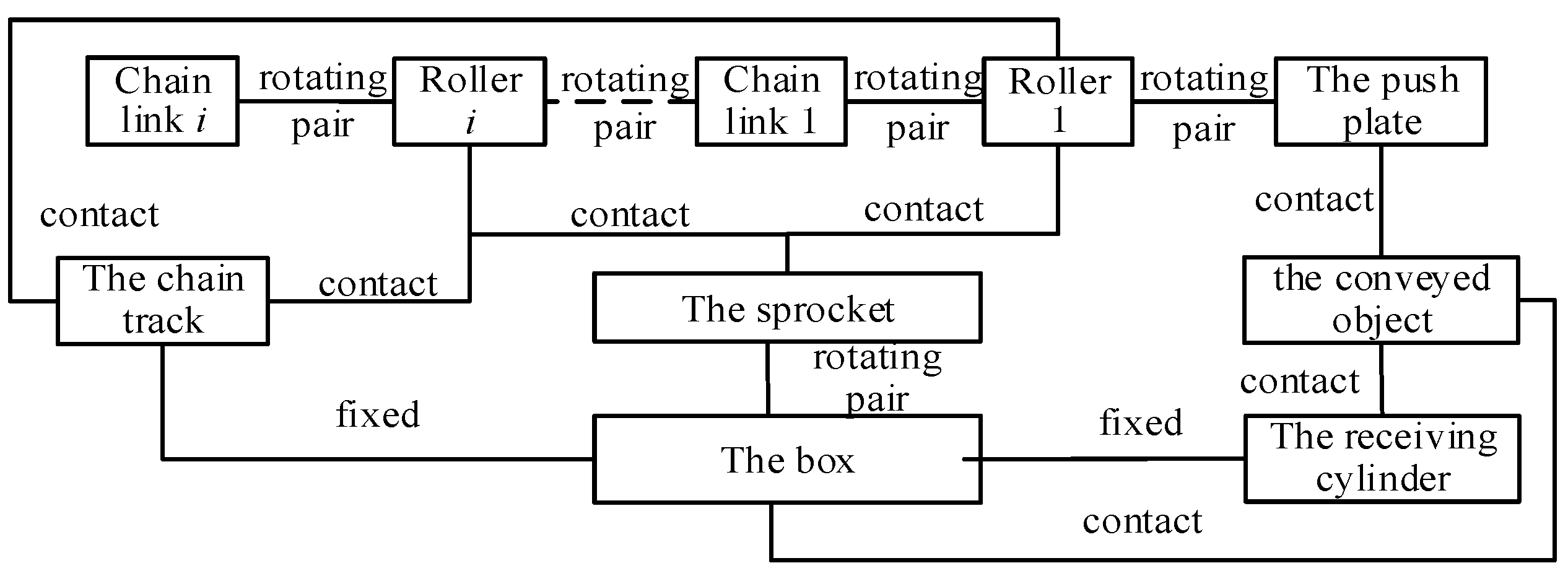
2. Dynamic Modeling of Chain Transmission Mechanism

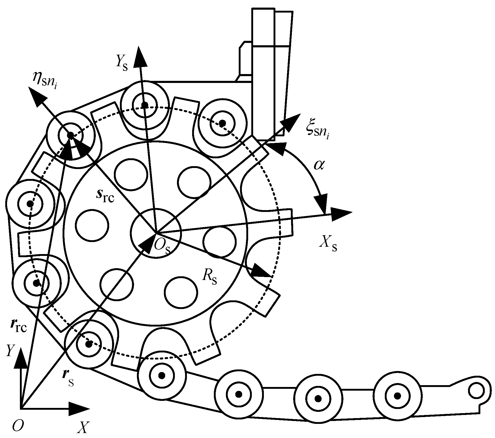
2.1. Model Description of Chain Transmission Mechanism

The research object of this paper is a chain transmission mechanism in a practical engineering application, as shown in Figure 1. It consists of an open-chain transmission system with non-interconnected ends (including rollers, chain links, pins, sprockets), a push plate, a transmission cylinder, chain track, the conveyed object, and a receiving cylinder. Driven by a transmission motor, the sprocket rotates and drives the chain forward. Ultimately, the push plate pushes the conveyed object into the receiving cylinder. The chain transmission system is a multi-degree-of-freedom system composed of multiple chain links connected by pins, where the pins’ two ends are rollers that contact the sprocket to achieve transmission, while the track constrains the rollers’ motion direction.

Based on the relative positions and connection relationships of the components of the chain transmission mechanism, the topological relationship is analyzed and shown in Figure 2. In the figure, the dashed lines represent the omitted chain links and rollers. The sprocket is installed on the box with a rotating pair, and there is a contact relationship between the sprocket and the roller. The roller is connected to the chain link through a rotating pair. The first chain link is a pushing plate, which contacts the conveyed object and pushes it forward. The track is fixed on the box and contacts the roller to constrain its movement.

2.2. Basic Assumptions

Based on the structural description, in order to establish a relatively accurate dynamic model of the chain transmission mechanism, the following assumptions need to be made first:

(1)

The system operates under steady-state conditions, and external disturbances are assumed to be negligible;

(2)

The chain transmission system is treated as a rigid body system, with no deformation of components during operation;

(3)

The friction between chain links, sprockets, and rollers is assumed to be constant for simplification;

(4)

The relationship between the rotational motion of the sprocket and the translational motion of the chain is idealized, assuming no slipping or stretching of the chain;

(5)

The chain transmission mechanism is treated as a planar system, considering only the motion within the plane and rotation about its axis of rotation.

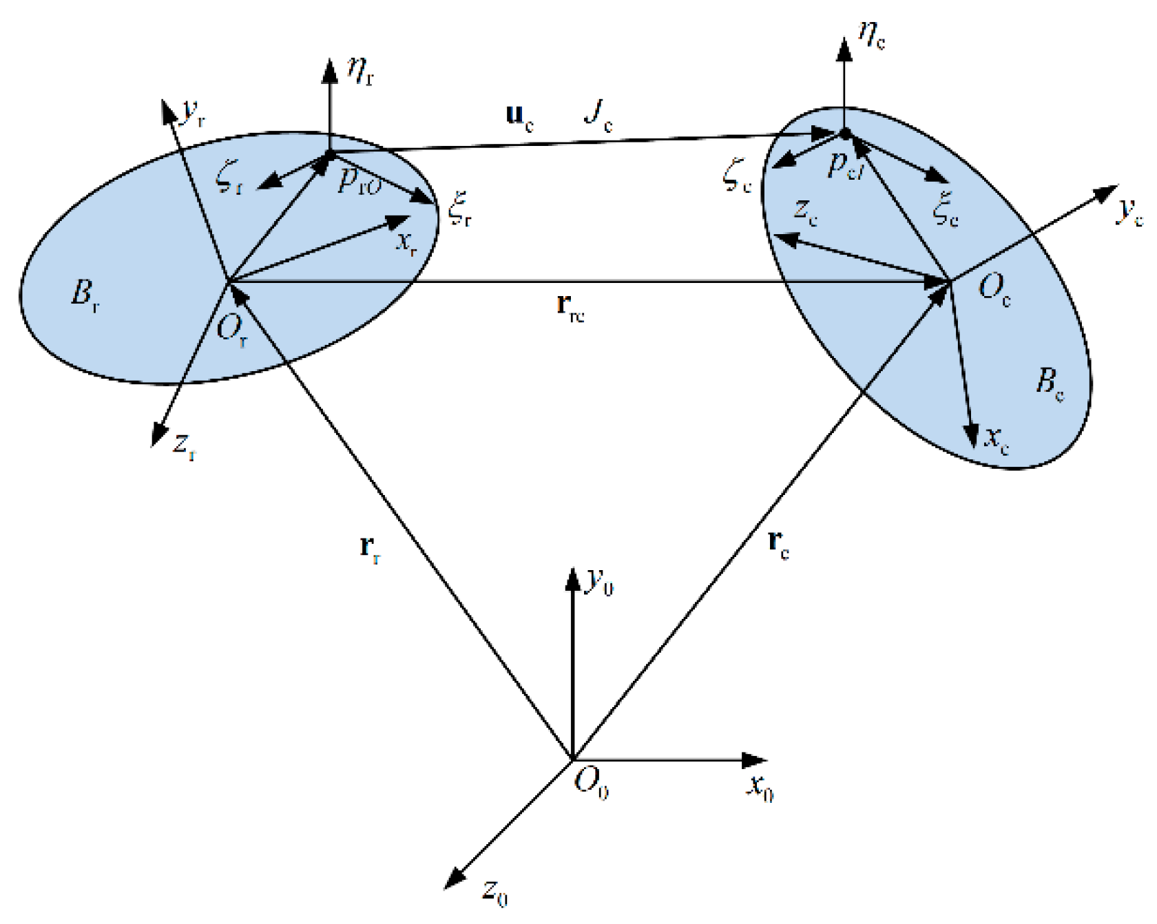
2.3. Motion and Contact Analysis of Open Chain System

From the topological relationship, it can be seen that there are numerous contact collisions in the model, including the contact collisions between the rollers and the sprocket teeth, between the rollers and the track, between the chain links, between the push plate and the conveyed object, etc. In order to establish a more accurate dynamic model of the chain transmission mechanism, it is necessary to analyze the above-mentioned contact collision processes.

The characteristics of the sprocket include the number of teeth $n_{\mathrm{t}}$, the original radius of the sprocket $R_{\mathrm{s}}$, and the pitch angle $\alpha$. A schematic diagram of the chain system is shown in Figure 3. In the figure, ${\mathit{r}}_{\mathrm{s}}={\left[x_{\mathrm{s}},y_{\mathrm{s}}\right]}^{\mathrm{T}}$ and represents the position vector of the sprocket’s center in the global coordinate system; ${\mathit{r}}_{\mathrm{rc}}={\left[x_{\mathrm{rc}},y_{\mathrm{rc}}\right]}^{\mathrm{T}}$ and represents the position vector of the roller $i$ in the global coordinate system $O-XY$; and ${\mathit{S}}_{\mathrm{rc}}$ represents the vector from the sprocket center to the roller center. The sprocket coordinate system $O_{\mathrm{s}}-X_{\mathrm{s}}{Y}_{\mathrm{s}}$ is located at the center of the sprocket, with the teeth numbered from $n_i=1$ counterclockwise, and $n_i$ represents the n-th tooth. For convenience, a local coordinate system $O_{\mathrm{s}}-{\xi }_{\mathrm{s}{n}_i}{\eta }_{\mathrm{s}{n}_i} ,\left(n_i=1,\cdots ,n_{\mathrm{t}}\right)$ for the tooth groove is established, and the rotation angle relative to the sprocket coordinate system at the origin $O_{\mathrm{s}}$ is denoted as ${\theta }_{\mathrm{s}}=\left(n_i-1\right)\alpha$. The coordinate transformation matrix from the $O_{\mathrm{s}}-{\xi }_{\mathrm{s}{n}_i}{\eta }_{\mathrm{s}{n}_i}$ to the $O_{\mathrm{s}}-X_{\mathrm{s}}{Y}_{\mathrm{s}}$ is given by

$${\mathit{A}}_{s{n}_i}=\left[\begin{array}{cc}\cos {\theta }_s& -\sin {\theta }_s\\ \sin {\theta }_s& \cos {\theta }_s\end{array}\right]$$

(1)

For convenience in calculation, all contact relationships between the rollers and the sprocket teeth are defined in the tooth groove coordinate system. When a vector is represented in the tooth groove coordinate system, any vector $\left(·\right)$ is expressed as ${\left(·\right)}^{″}$. For example, the vector from the center of the sprocket to the center of the roller is defined as

$${\mathit{s}}_{\mathrm{rc}}={\mathit{r}}_{\mathrm{rc}}-{\mathit{r}}_s$$

(2)

and represented in the tooth groove coordinate system as

$${\mathit{s}}_{\mathrm{rc}}^{″}={\mathit{A}}_{s{n}_i}^T{\mathit{s}}_{\mathrm{rc}}$$

(3)

The schematic diagram of the sprocket tooth profile is shown in Figure 4. To reduce the impact during the meshing process between the roller and the sprocket tooth groove, the sprocket tooth groove is typically composed of several continuous curved surfaces [26,27]. To accurately represent the contact relationship between the roller and the sprocket tooth groove, the tooth groove is divided into three regions: the tooth groove positioning curve (bottom curve) bc, and the top transition curve ab and cd. The center of the curvature is defined as $o_{ab}$, $o_{bc}$, and $o_{cd}$, and the radius of the circular arcs in the respective segments ab and cd are $R_1$, and in the respective segment bc is $R_2$, respectively.

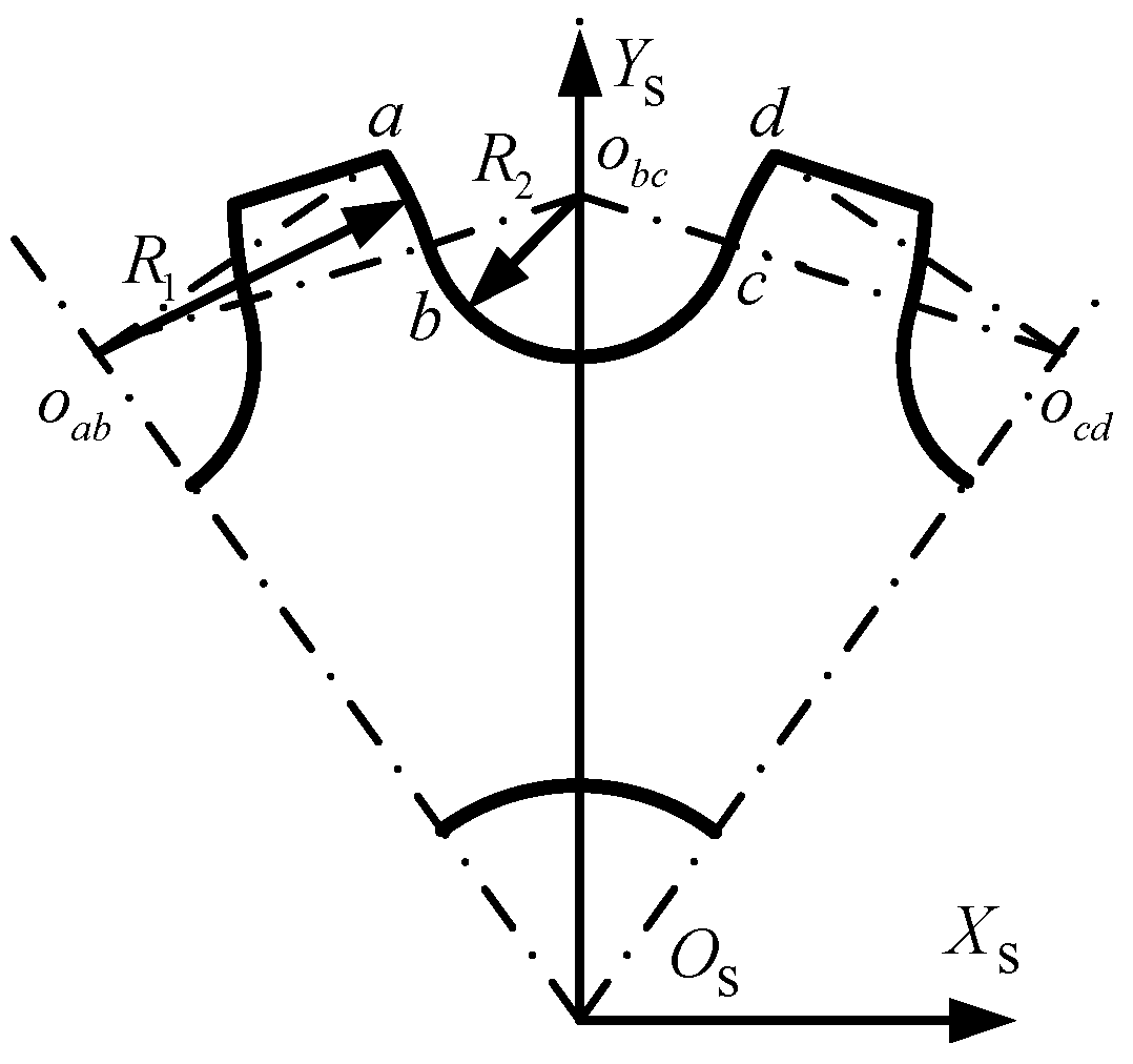
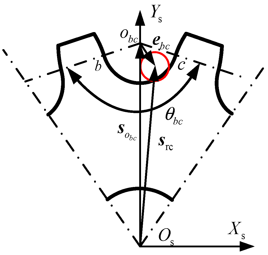
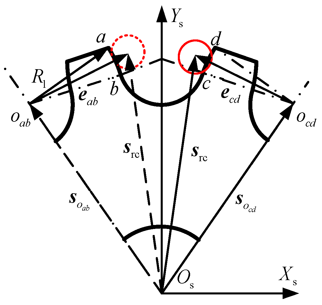
2.3.1. Geometric Relationship Between the Sprocket Tooth Groove and the Roller Contact

Under normal operating conditions, the contact between the roller and the sprocket occurs at different positions on the sprocket tooth groove. Therefore, to accurately calculate the kinematic and dynamic relationship between the roller and the sprocket tooth groove, it is necessary to describe the contact relationship between the roller and the different arc segments separately.

As shown in Figure 5, the schematic diagram illustrates the contact relationship between the roller and the sprocket tooth groove positioning curve. The eccentric vector ${\mathit{e}}_{bc}$ is the vector between the center of the roller and the center of the bottom arc, expressed as

$${\mathit{e}}_{bc}={\mathit{s}}_{\mathrm{rc}}-{\mathit{s}}_{o_{bc}}$$

(4)

where ${\mathit{s}}_{o_{bc}}$ is the vector from the center of the bottom arc to the center of the sprocket.

In Figure 5, ${\theta }_{bc}$ represents the angle of arc segment bc relative to the center $o_{bc}$.

Let ${\theta }_2$ represent the angle between ${\mathit{e}}_{bc}$ and $-{\mathit{s}}_{o_{bc}}$, then

$${\theta }_2=\arccos {\displaystyle \frac{-{\mathit{s}}_{o_{bc}}{\mathit{e}}_{bc}}{‖-{\mathit{s}}_{o_{bc}}‖‖{\mathit{e}}_{bc}‖}}$$

(5)

The contact constraint occurring at the bottom arc is

$$-{\displaystyle \frac{1}{2}}{\theta }_{bc}<{\theta }_2<{\displaystyle \frac{1}{2}}{\theta }_{bc}$$

(6)

If the above equation is not satisfied, check whether contact occurs at other positions; if ${\theta }_2$ is positive, check if contact occurs on the arc segment cd; if ${\theta }_2$ is negative, check if contact occurs on the other arc segment ab. If the above equation is satisfied, calculate the penetration ${\delta }_{bc}$ between the roller and the sprocket tooth groove positioning curve according to Equation (7)

$${\delta }_{bc}=‖{\mathit{e}}_{bc}‖-\left(R_2-R_{\mathrm{r}}\right)$$

(7)

where $R_{\mathrm{r}}$ is the radius of the roller.

If both Equation (6) and the condition ${\delta }_{bc}\ge 0$ are satisfied, the contact between the roller and the sprocket tooth groove occurs on the arc segment bc; otherwise, there is no contact between the roller and the sprocket tooth groove on the arc segment bc.

Figure 6 is a schematic diagram of the contact relationship between the roller and the top transition curve of the sprocket tooth groove. The top transition curve of the sprocket tooth groove consists of an arc segment ab and another arc segment cd, so both arc segments need to be analyzed separately.

In Figure 6, ${\mathit{e}}_{ab}$ and ${\mathit{e}}_{cd}$ represent the eccentric vectors from the center of the arc segment ab to the center of the roller, and from the center of the arc segment cd to the center of the roller, respectively. ${\mathit{s}}_{o_{ab}}$ and ${\mathit{s}}_{o_{cd}}$ represent the position vectors from the center of the arc segment ab and the center of the arc segment cd to the center of the sprocket, respectively.

Based on the different arc segments, the positional relationship between the roller and the top transition curve of the sprocket tooth groove can be described as follows:

(1) When the roller contacts the top transition curve of the sprocket tooth groove, assuming contact occurs at arc segment ab, we obtain

$${\mathit{e}}_{ab}={\mathit{s}}_{\mathrm{rc}}-{\mathit{s}}_{o_{ab}}$$

(8)

Let $T_{\mathrm{e}}$ represent the angle between ${\mathit{s}}_{o_{ab}a}$ and ${\mathit{e}}_{ab}$, where ${\mathit{s}}_{o_{ab}a}$ represents the position vector from the point $o_{ab}$ to the point a, then

$${\theta }_1=\arccos \left({\displaystyle \frac{{\mathit{s}}_{o_{ab}a}{\mathit{e}}_{ab}}{‖{\mathit{s}}_{o_{ab}a}‖‖{\mathit{e}}_{ab}‖}}\right)$$

(9)

Let $R_{\mathrm{r}}$ represent the angle between ${\mathit{s}}_{o_{ab}b}$ and ${\mathit{e}}_{ab}$, where ${\mathit{s}}_{o_{ab}b}$ represents the position vector from the point $R_{\mathrm{m}}$ to the point b, then

$${\theta }_1^{\prime }=\arccos \left({\displaystyle \frac{{\mathit{s}}_{o_{ab}b}{\mathit{e}}_{ab}}{‖{\mathit{s}}_{o_{ab}b}‖‖{\mathit{e}}_{ab}‖}}\right)$$

(10)

The contact constraint occurring at arc segment ab is

$$\left\{\begin{array}{l}0\le {\theta }_1<{\theta }_{ab}\\ 0\le {\theta }_1^{\prime }<{\theta }_{ab}\end{array}\right.$$

(11)

where ${\theta }_{ab}$ represents the angle corresponding to arc segment ab relative to the center $T_{\max }$ of the circle.

If Equation (11) is satisfied, the penetration ${\delta }_{ab}$ between the roller and the top transition curve of the sprocket tooth groove for arc segment ab is calculated as

$${\delta }_{ab}=R_1-\left(‖{\mathit{e}}_{ab}‖-R_{\mathrm{r}}\right)$$

(12)

If both Equation (11) and the condition ${\delta }_{ab}\ge 0$ are satisfied, the roller contacts the top transition curve of the sprocket tooth groove at arc segment ab. Otherwise, there is no contact between the roller and the top transition curve of the sprocket tooth groove at arc segment ab.

(2) When the roller contacts the top transition curve of the sprocket tooth groove at arc segment cd, the contact constraint for arc segment cd is given by

$$\left\{\begin{array}{l}0<{\theta }_3\le {\theta }_{cd}\\ 0<{\theta }_3^{\prime }\le {\theta }_{cd}\end{array}\right.$$

(13)

where ${\theta }_{cd}$ represents the angle corresponding to arc segment cd relative to the center $o_{cd}$ of the circle.

If Equation (13) is satisfied, the penetration between the roller and the top transition curve of the sprocket tooth groove for arc segment cd is calculated as

$${\delta }_{cd}=R_1-\left(‖{\mathit{e}}_{cd}‖-R_{\mathrm{r}}\right)$$

(14)

If both Equation (13) and the condition ${\delta }_{cd}\ge 0$ are satisfied, the roller contacts the top transition curve of the sprocket tooth groove at arc segment cd; otherwise, there is no contact between the roller and the top transition curve of the sprocket tooth groove at arc segment cd.

2.3.2. Contact Between Chain Links

In order to use the chain links to drive an object forward, it is necessary to add planar constraints between the chain links. At the initial moment, the chain links are in the chain box. When the chain links rotate over the sprocket and reach above the sprocket, under the action of planar constraints, the planes of the two-chain links will come into contact. The critical condition for contact is when the upper surfaces of the two-chain links are parallel. As shown in Figure 7, for two adjacent chain links $O_{\mathrm{c}k}$ and $O_{\mathrm{c}\left(k+1\right)}$, the angle between the two coordinate axes $O_{\mathrm{c}k}{Y}_{\mathrm{c}k}$ and $O_{\mathrm{c}\left(k+1\right)}{Z}_{\mathrm{c}\left(k+1\right)}$ is $\gamma$, and the condition for contact between the two chain links is as follows

$$\gamma \le {\displaystyle \frac{\mathsf{\pi }}{2}}$$

(15)

In Figure 7, points P and Q are the points at the top of the chain link contact plane. ${\mathit{r}}_{PQ}$ is the position vector from point P to point Q; ${\mathit{r}}_Q$ is the position vector from the origin of the global coordinate system to point Q; and ${\mathit{r}}_P$ is the position vector from the origin of the global coordinate system to point P. When the two-chain links come into contact, the contact area is a planar rectangular region. Since the connection between the chain link and the roller is a rotating pair, the contact between the two-chain links will always occur at the upper end first. Due to the influence of the rotational angle, in order to ensure the rationality of the penetration calculation, the penetration depth at the upper end is taken as half of the actual penetration depth (as shown in Figure 7). Therefore, the penetration is given by

$${\mathsf{\delta }}_{\mathrm{p}}={\displaystyle \frac{{\mathit{r}}_{PQ}}{2}}={\displaystyle \frac{{\mathit{r}}_Q-{\mathit{r}}_P}{2}}$$

(16)

Based on Equation (16), the magnitude of the penetration is given by

$${\delta }_{\mathrm{p}}=\sqrt{{\mathsf{\delta }}_{\mathrm{p}}^{\mathrm{T}}{\mathsf{\delta }}_{\mathrm{p}}}$$

(17)

Furthermore, based on the magnitude and direction of the penetration, the contact collision force between the chain links can be calculated.

2.4. Contact Force Model

The motion constraints between the roller and the sprocket, as well as between the roller and the track, are established through contact theory [28,29]. The contact force model for the arc surface is described using the Lankarani–Nikravesh model, as shown in Equation (18). The planar contact force [30] is described as in Equation (19), and the tangential friction force [31] is modeled using Coulomb’s model, as shown in Equation (20). The kinematic relationship between the head and tail components, as well as the last component of the closed-loop transmission chain, is established using the cut-joint method [32].

$$F_{\mathrm{n}}=K{h}^n+C\dot{h}$$

(18)

$$F_{\mathrm{np}}=K_{\mathrm{p}}{\mathsf{\delta }}_{\mathrm{p}}$$

(19)

$$F_{\mathrm{t}}=-c_{\mathrm{f}}{c}_{\mathrm{d}}{F}_{\mathrm{n}}{\displaystyle \frac{{\mathit{v}}_{\mathrm{t}}}{‖{\mathit{v}}_{\mathrm{t}}‖}}$$

(20)

where, $F_{\mathrm{n}}$ is the normal collision force; K is the stiffness coefficient of the two contacting bodies; h is the penetration depth of the contact bodies; n is the contact index; C is the contact damping coefficient; $\dot{h}$ is the relative collision velocity at the contact point; ${\delta }_{\mathrm{p}}$ is the planar contact penetration depth; $K_{\mathrm{p}}$ is the equivalent stiffness of the planar contact; $F_{\mathrm{t}}$ is the tangential friction force; $c_{\mathrm{f}}$ is the coefficient of sliding friction; $c_{\mathrm{d}}$ is the dynamic correction factor; and ${\mathit{v}}_{\mathrm{t}}$ is the relative tangential velocity.

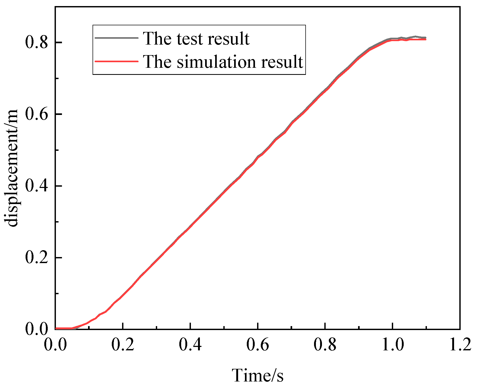
2.5. Dynamic Model and Experimental Validation of Chain Transmission Mechanism

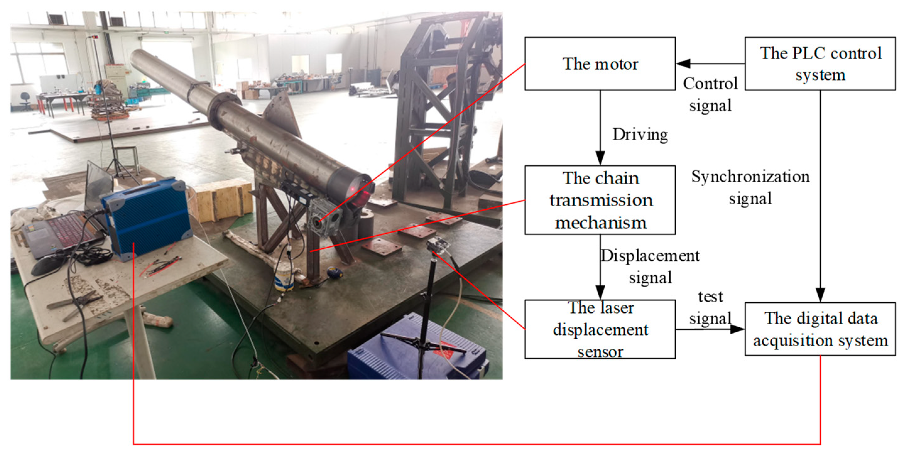
Based on the kinematic relationships, forces, and constraints of the chain transmission mechanism, and using the principle of virtual work [31], the dynamic equations of the chain transmission mechanism are established as follows: (see Appendix A for modeling details)

$$\left\{\begin{array}{l}\mathit{M}\left(\mathit{q},t\right)\ddot{\mathit{q}}+\mathit{C}\left(\mathit{q},\dot{\mathit{q}},t\right)\dot{\mathit{q}}+{\mathit{\Phi }}_{\mathit{q}}^{\mathrm{T}}\lambda =\mathit{Q}\\ \mathit{\Phi }\left(\mathit{q},t\right)=\mathit{0}\end{array}\right.$$

(21)

where, t is the motion time of the transmission process, $\mathit{q}$, $\dot{\mathit{q}}$, and $\ddot{\mathit{q}}$ represent the relative displacement, relative velocity, and relative acceleration of the rotational joints in the chain transmission mechanism, respectively. $\mathit{\Phi }\left(\mathit{q},t\right)=\mathit{0}$ is the constraint equation of the chain transmission mechanism, ${\mathit{\Phi }}_{\mathit{q}}$ denotes the derivative of $\mathit{\Phi }\left(\mathit{q},t\right)$ with respect to $\mathit{q}$, and ${\left(·\right)}^{\mathrm{T}}$ represents the transpose of the matrix. $\lambda$ is the Lagrange multiplier, $\mathit{M}\left(\mathit{q},t\right)$ is the mass matrix of the chain transmission mechanism, $\mathit{C}\left(\mathit{q},\dot{\mathit{q}},t\right)$ is the generalized damping matrix of the chain transmission mechanism, and $\mathit{Q}$ is the external force acting on the chain transmission mechanism.

To verify the accuracy and effectiveness of the simulation model, experimental tests are conducted on the chain transmission process. The experimental setup mainly consists of a chain transmission mechanism test rig, a PLC control system, a digital data acquisition system, a laser displacement sensor, etc., as shown in Figure 8. The PLC control system serves as the drive execution system for the chain transmission mechanism and records the motor current in real time. The digital acquisition device reads and records the displacement of the conveyed object as measured by the laser displacement sensor, while also receiving synchronization signals from the PLC.

The experimental process is as follows:

(1)

According to the schematic diagram in Figure 8, arrange the experimental setup and connect the testing system. The data acquisition system is connected to the PLC control system to ensure the synchronization of the data signals. The displacement sensor is mounted at the rear of the chain transmission mechanism using a bracket. The sensor captures the laser signal of the moving conveyed object, and the displacement sensor is connected to the data acquisition system.

(2)

Power up the control system. Under the drive of the motor, the chain transmission mechanism moves the conveyed object forward. The PLC control system collects the current, while the data acquisition system collects the signals from the displacement sensor and the PLC’s synchronization signals.

(3)

To minimize the impact of external disturbances on parameter uncertainty, perform the test three times under the same conditions.

(4)

Data collection and processing: Export data from the PLC control system and data acquisition software (TranAX_3.4.1.1222, the USA). Extract valid data during the motion process of the conveyed object to conduct subsequent dynamic simulations and experimental comparisons. Then, take the average of the three data sets under the same operating conditions.

Through bench tests, the current $i_{\mathrm{q}}$ of the chain transmission mechanism is obtained. Based on the motor electromagnetic torque equation, the motor torque $T_{\mathrm{e}}$ can be expressed as

$$T_{\mathrm{e}}=K_{\mathrm{T}}{i}_{\mathrm{q}}$$

(22)

where $K_{\mathrm{T}}$ is the motor torque constant. The motor torque is transmitted to the sprocket shaft through the worm gear transmission mechanism, with a transmission ratio of k. Therefore, the torque on the sprocket is given by

$$T_{\mathrm{s}}=k{T}_{\mathrm{e}}$$

(23)

The current driven by the motor during the transmission process is obtained through bench tests. The motor torque is then converted into the sprocket torque using Equation (23). As shown in Figure 9, for ease of analysis, the sprocket torque is approximated and represented by the red line in the figure. The converted sprocket torque is then input into the simulation dynamic model of the chain transmission mechanism, and the simulation results for the displacement of the transmitted object are compared with experimental results, as shown in Figure 10. From Figure 10, it can be seen that the simulation results are in good agreement with the experimental data. This validates the correctness and effectiveness of the model. In subsequent calculations, this simulation model will be used to replace the real physical model for analysis.

3. Robust Optimization Design Model for Chain Transmission Process Considering Random Loads

3.1. Random Parameters of the Chain Transmission Process

Based on design requirements and engineering experience, the random parameters considered in this paper for the chain transmission mechanism include the following.

(1)

Structural dimension parameters: roller radius $R_{\mathrm{r}}$, sprocket tooth groove radius $R_1$, sprocket transition arc radius $R_2$, initial position of the transmitted object relative to the end face of the receiving cylinder $L_{\mathrm{m}}$, transmission cylinder radius $R_{\mathrm{t}}$, and the inner diameter of the receiving cylinder $R_{\mathrm{s}}$. To enhance the robustness of the chain transmission mechanism, the above structural dimension parameters are treated as design parameters, while considering the influence of parameter random fluctuations.

(2)

Physical property parameters: the coefficient of friction between the transmitted object and the transmission track and receiving cylinder ${\mu }_s$, and the mass of the transmitted object $m_{\mathrm{m}}$. These parameters also have an influence on the positioning consistency of the transmitted object but are difficult to design. Therefore, they are not considered as design parameters, and only the effect of random fluctuations in these parameters is taken into account.

(3)

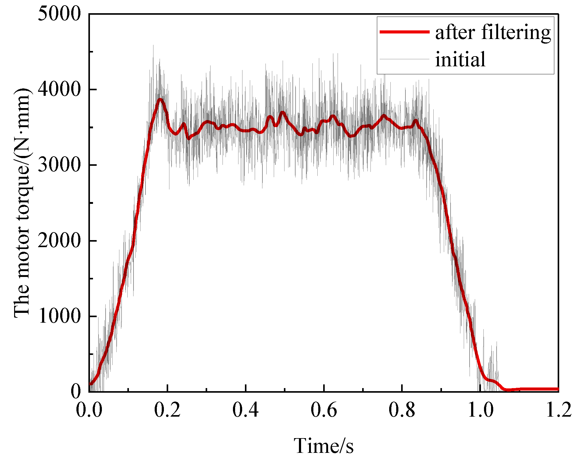
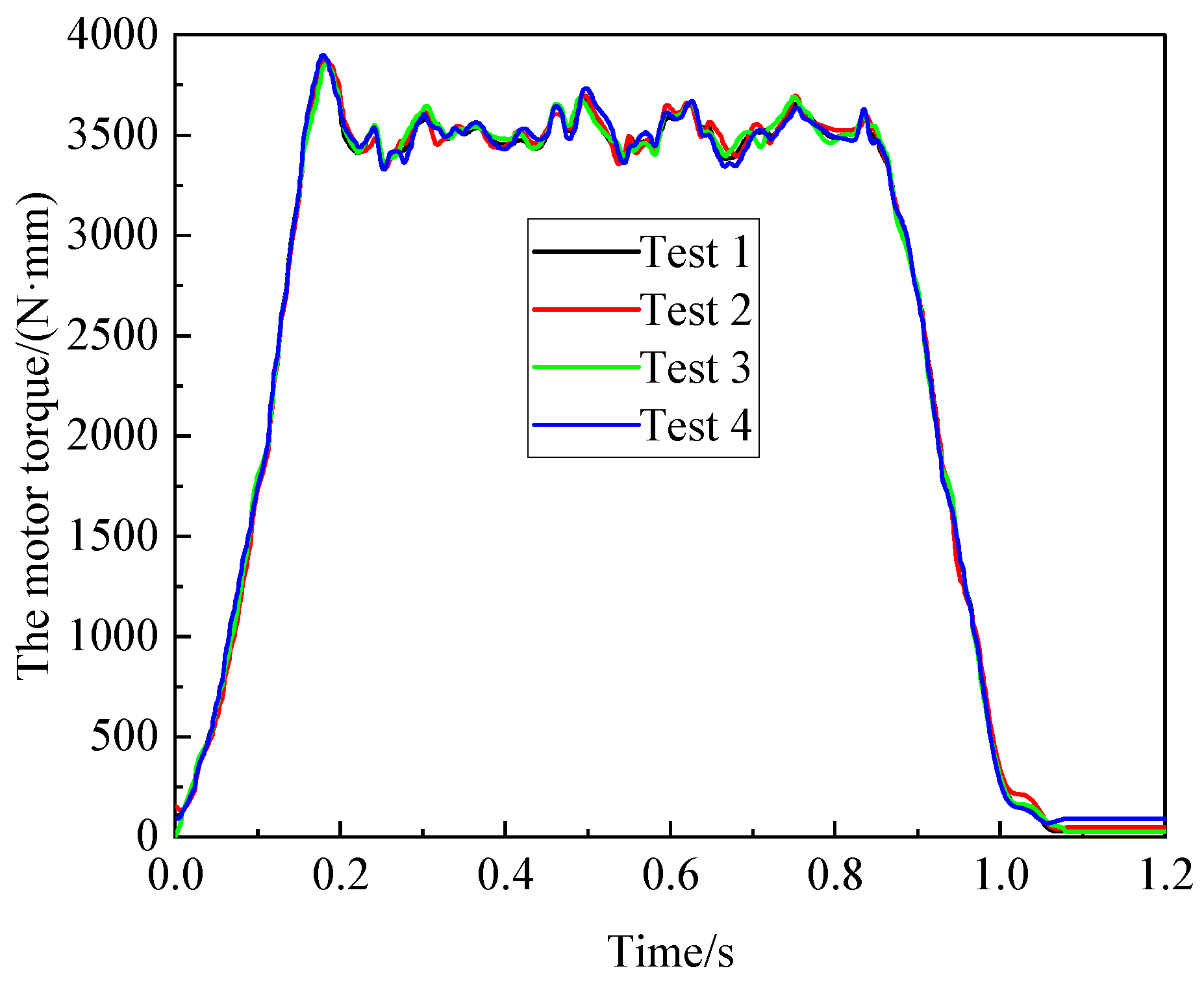
Time-varying random loads: Based on the multiple torque curves after tests (Figure 11), it is observed that although the same motor speed is given, the driving load exhibits time-varying uncertainty. The fluctuations in the load have a significant effect on the positioning accuracy of the chain transmission mechanism. Therefore, the effect of time-varying random loads is considered.

To achieve robust design of the chain transmission mechanism, the parameters are classified into controllable and uncontrollable parameters based on whether the uncertain input parameters can be controlled. Controllable parameters refer to those that can be easily altered during the design and manufacturing process, while uncontrollable parameters are those that are difficult or impossible to change during design and manufacturing. Among the controllable parameters, there are random variables ${\mathit{X}}_{\mathrm{v}}=\left[R_1,R_2,R_{\mathrm{t}},R_{\mathrm{s}},R_{\mathrm{r}},L_{\mathrm{m}}\right]$ and non-random variables ${\mathit{X}}_{\mathrm{c}}=\left[\right]$. Similarly, the uncontrollable parameters are also classified into random variables ${\mathit{P}}_{\mathrm{v}}=\left[m_{\mathrm{m}},{\mu }_{\mathrm{s}}\right]$ and non-random variables ${\mathit{P}}_{\mathrm{c}}=\left[R_{\mathrm{m}}\right]$.

3.2. Random Driving Load Analysis Based on Karhunen–Loeve Expansion

In multiple chain transmission processes under the same working conditions, the driving load exhibits certain fluctuations, and thus, can be treated as a dynamic random process. To ensure the accuracy of the effect of the driving load on the positioning accuracy of the conveyed object, the sampling time interval is generally set to 0.001 s. As a result, the entire random process of the driving load is discretized into thousands of random variables, which poses significant challenges for the subsequent uncertainty propagation of this dynamic uncertain parameter. To address this, this paper adopts the Karhunen–Loeve expansion (K-L expansion) method [33], which reduces the dimensionality of the time series random driving load with correlation, thereby providing strong support for the subsequent uncertainty propagation. It should be noted that the K-L expansion relies on the covariance matrix, which requires knowledge of the complete covariance structure in the problem. In the theory of random processes, the K-L expansion represents the random dynamic load as an infinite linear combination of orthogonal functions based on the spectral decomposition of the covariance function. Considering the probability space of the driving load, the covariance function of the random process $P\left(t\right)$ within the bounded interval [0, T] is $C\left(t_m,t_n\right)$, and the process can be expressed as

$$P\left(t\right)={\mu }_P\left(t\right)+{\displaystyle \sum _{i=1}^{\infty }\sqrt{{\gamma }_i}{\xi }_i{\phi }_i\left(t\right)}$$

(24)

where, $t\in \left[0,T\right]$, ${\mu }_P\left(t\right)$ is the mean function of the driving load random process, and ${\xi }_i$ represents i-th mutually independent standard random variable. ${\gamma }_i$ and ${\phi }_i\left(t\right)$ are the i-th eigenvalue and eigenfunction of the covariance function of the driving load random process, respectively. According to Mercer’s theorem [33], the covariance function has the following spectral decomposition:

$$C\left(t_m,t_n\right)={\displaystyle \sum _{i=1}^{\infty }{\gamma }_i{\phi }_i\left(t_m\right){\phi }_i\left(t_n\right)}$$

(25)

The eigenvalues ${\gamma }_i$ and eigenfunctions ${\phi }_i\left(t\right)$ can be obtained by solving the following second-kind Fredholm integral equation

$${\displaystyle {\int }_0^{T}C\left(t_m,t_n\right){\phi }_i\left(t_n\right)}d{t}_m={\gamma }_i{\phi }_i\left(t_n\right)$$

(26)

and satisfies

$${\displaystyle \sum _{j=1}^{\infty }{\gamma }_j}=\left|T\right|$$

(27)

The eigenfunctions in Equation (26) form a complete orthogonal set that satisfies the equation.

$${\displaystyle {\int }_0^T{\phi }_i\left(t\right){\phi }_j\left(t\right)}={\delta }_{ij}$$

(28)

In Equation (28), ${\delta }_{ij}$ is the Kronecker delta function. For uncorrelated standard random variables ${\xi }_i$, they can be obtained by the following equation:

$${\xi }_i={\displaystyle \frac{1}{\sqrt{{\gamma }_i}}}{\displaystyle {\int }_0^T\left[P\left(t\right)-{\mu }_P\left(t\right)\right]{\phi }_i\left(t\right)dt}$$

(29)

In the analysis of random driving loads in the chain transmission mechanism, the eigenvalues are often arranged in descending order, and the random process is approximated by a finite number of terms. For example, the truncated random process after M terms can be expressed as

$$\tilde{P}\left(t\right)={\mu }_P\left(t\right)+{\displaystyle \sum _{i=1}^M\sqrt{{\gamma }_i}{\xi }_i{\phi }_i\left(t\right)}$$

(30)

Its covariance expansion function is

$$C\left(t_m,t_n\right)={\displaystyle \sum _{i=1}^M{\gamma }_i{\phi }_i\left(t_m\right){\phi }_j\left(t_n\right)}$$

(31)

The error ${\epsilon }_{\mu }\left(t\right)$ in the mean function of the approximate random process $\tilde{P}\left(t\right)$ of the load and the mean squared error ${\overline{\epsilon }}_U^2\left(t\right)$ can be expressed as

$${\epsilon }_{\mu }\left(t\right)={\mu }_P\left(t\right)-{\tilde{\mu }}_P\left(t\right)\equiv 0$$

(32)

$${\overline{\epsilon }}_U^2\left(t\right)={\displaystyle \frac{1}{T}}{\displaystyle {\int }_T\left(\frac{{\displaystyle \sum _{i=1}^{\infty }\sqrt{{\gamma }_i}{\xi }_i{\phi }_i\left(t\right)}}{\sigma \left(t\right)}-\frac{{\displaystyle \sum _{i=1}^M\sqrt{{\gamma }_i}{\xi }_i{\phi }_i\left(t\right)}}{\sigma \left(t\right)}\right)}dt\le 1-{\displaystyle \frac{1}{\left|T\right|}}{\displaystyle \sum _{i=1}^{\infty }{\lambda }_j}$$

(33)

Therefore, the approximation degree $\kappa$ of the load random process can be defined as

$$\kappa ={\displaystyle \frac{1}{\left|T\right|}}{\displaystyle \sum _{j=1}^M{\lambda }_j}$$

(34)

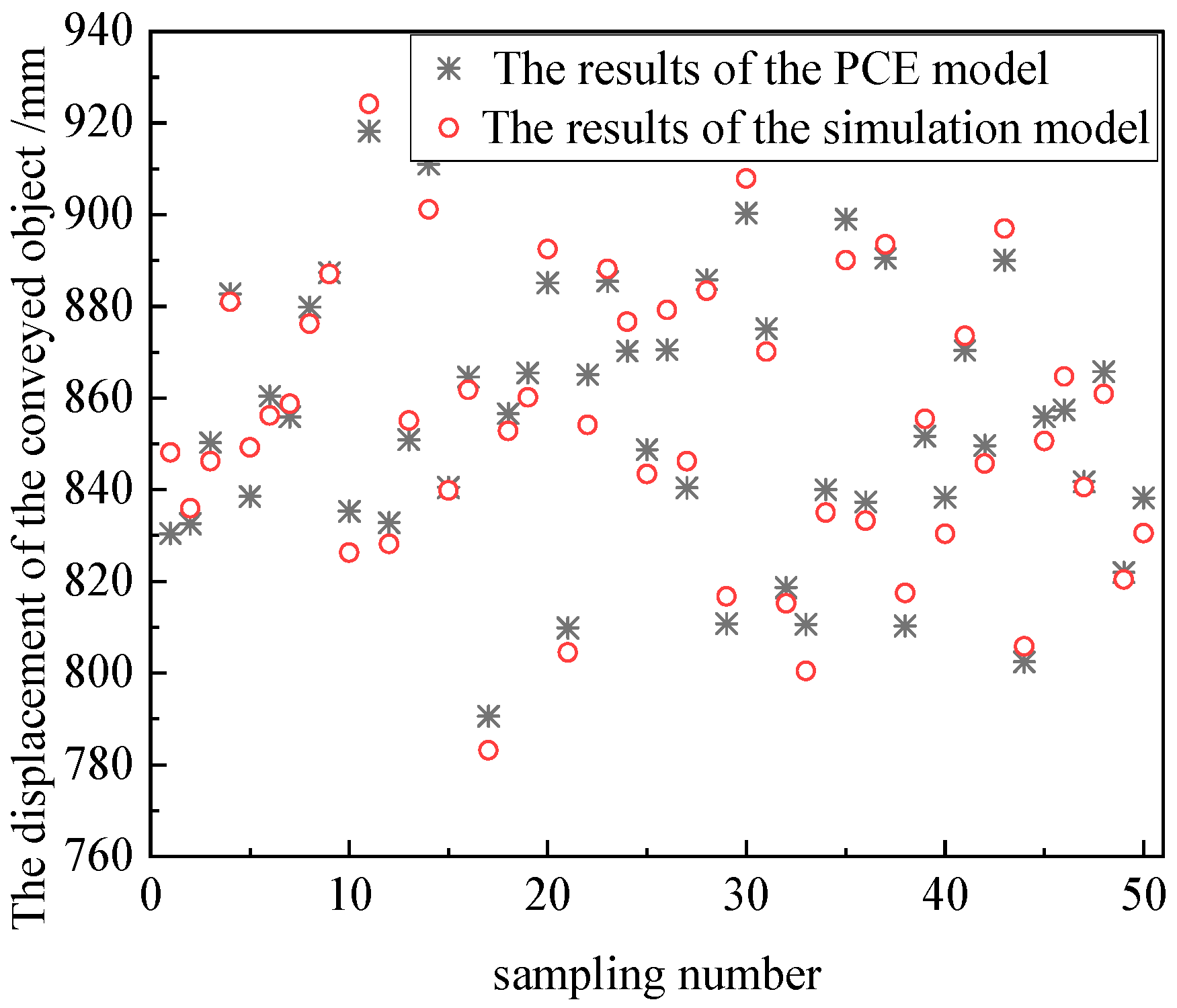
3.3. Chain Transmission Mechanism Surrogate Model Based on Polynomial Chaos Expansion

Due to the high non-linearity of the chain transmission mechanism model and the long computation time for each run, multiple model evaluations are required during the robust optimization design process, which significantly increases the computational cost. To reduce the computational cost while ensuring accuracy, this paper uses the Polynomial Chaos Expansion (PCE) model to establish a surrogate model for the chain transmission mechanism. It should be noted that high-order polynomial terms in PCE will rapidly increase computational complexity, especially when there are many random variables in the problem, the number of expanded terms will increase exponentially. Moreover, PCE assumes that random variables follow certain known probability distributions (usually normal or uniform), and its effectiveness may be poor for uncertainties with heavy tailed distributions (such as Laplace distributions).

The idea of constructing a surrogate model for the chain transmission mechanism using PCE [34] is to expand the output response of the chain transmission mechanism into a form of orthogonal polynomials corresponding to e uncertainty input parameters. Let the i-th input parameter of the chain transmission mechanism be denoted as $x_i=\left[a_i,b_i\right],\left(i=1,2,\cdots ,e\right)$, and its probability distribution function corresponding to the standard orthogonal polynomial $\Psi \left({\tilde{x}}_i\right)$. Here, ${\tilde{x}}_i$ represents the definition of the input parameter ${\tilde{x}}_i$ in the corresponding chaos polynomial space, and the corresponding value range is ${\tilde{x}}_i=\left[c_i,d_i\right],\left(i=1,2,\cdots ,e\right)$.

The input parameters $x_i$ of the chain transmission mechanism and their corresponding definitions ${\tilde{x}}_i$ in the chaos polynomial space satisfy the following relationship:

$${\tilde{x}}_i={\displaystyle \frac{d_i-c_i}{b_i-a_i}}{x}_i+{\displaystyle \frac{c_i{b}_i-a_i{d}_i}{b_i-a_i}}$$

(35)

Based on the idea of sparse chaos polynomials, the output response $y=f\left(\mathit{x}\right)$ of the chain transmission mechanism is expanded into a series of finite order $s$, expressed as a sum of orthogonal polynomials of the input parameters, as follows:

$$y=f\left(\mathit{x}\right)={\displaystyle \sum _{g=1}^s{\beta }_g{\varphi }_{{\mathit{u}}_g}\left(\tilde{\mathit{x}}\right)}$$

(36)

$${\varphi }_{{\mathit{u}}_g}\left(\tilde{\mathit{x}}\right)={\displaystyle \prod _{h=1}^e{\Psi }_{u_{gh}}\left({\tilde{x}}_h\right)}$$

(37)

where, ${\beta }_g$ is the polynomial expansion coefficient, ${\varphi }_{{\mathit{u}}_g}\left(\tilde{\mathit{x}}\right)$ is the multi-variate polynomial, $u_{gh}$ is the degree of the polynomial ${\Psi }_{u_{gh}}\left({\tilde{x}}_h\right)$, s is the total number of chaos polynomial expansion terms, and ${\mathit{u}}_g$ is the set of polynomial degrees.

According to the orthogonality property of the orthogonal polynomials, the following can be obtained:

$$〈{\varphi }_{{\mathit{u}}_g}\left(\tilde{\mathit{x}}\right),{\varphi }_{{\mathit{u}}_h}\left(\tilde{\mathit{x}}\right)〉=〈{\varphi }_{{\mathit{u}}_g}{\left(\tilde{\mathit{x}}\right)}^2〉{\delta }_{gh}$$

(38)

where $〈·〉$ denotes the inner product with the joint probability density function as the weight function, ${\delta }_{gh}$ is the Kronecker delta function, and if g = h, then ${\delta }_{gh}=1$; otherwise, ${\delta }_{gh}=0$.

Based on Equation (36), the PCE model of the chain transmission mechanism can be obtained. However, due to the large number of PCE terms, the computational load has increased. To address this issue, reference [35] proposes a sparse chaos polynomial expansion strategy to reduce the number of PCE terms. The Elastic Net (EN) method is used to identify the terms in the PCE model that are important to the result, thus improving computational efficiency while maintaining accuracy. The polynomial coefficient ${\tilde{\mathit{\beta }}}_{\mathrm{EN}}$ is then represented as

$${\tilde{\mathit{\beta }}}_{\mathrm{EN}}=\arg \underset{\beta }{\min }\left({‖Y-{\mathit{\varphi }}_{\mathit{u}}^{\mathrm{T}}\tilde{\mathit{\beta }}‖}_2+{\lambda }_1{‖\tilde{\mathit{\beta }}‖}_1+{\lambda }_2{‖\tilde{\mathit{\beta }}‖}_2\right)$$

(39)

where $\arg \underset{\beta }{\min }\left(·\right)$ denotes the minimization functional, ${\lambda }_1$ and ${\lambda }_2$ are adjustment parameters, Y is the output, ${\mathit{\varphi }}_{\mathit{u}}^{\mathrm{T}}$ is the transpose of the multi-variate polynomial set, and $\tilde{\mathit{\beta }}$ represents the set of polynomial coefficients. The Least Angle Regression (LAR) algorithm [36] is used to improve the computational efficiency of the EN method. The final SPCE surrogate model is then expressed as

$$y={\mathit{\varphi }}_{\mathit{B}}^{\mathrm{T}}\left(\tilde{\mathit{x}}\right){\tilde{\mathit{\beta }}}_{\mathrm{EN}}$$

(40)

where ${\mathit{\varphi }}_{\mathit{B}}^{\mathrm{T}}\left(\tilde{\mathit{x}}\right)$ is the set of multi-variate polynomials retained after EN selection.

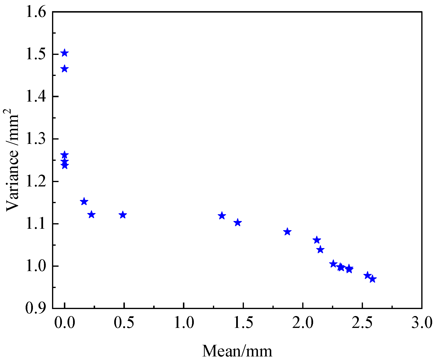
3.4. Robust Optimization Design Model for Chain Transmission Mechanism

Considering the effect of the random variation of uncontrollable parameters ${\mathit{P}}_{\mathrm{v}}$, and given the value of the non-random variation of the uncontrollable parameters ${\mathit{P}}_{\mathrm{c}}$, with controllable parameters $\mathit{X}$ (including both ${\mathit{X}}_{\mathrm{v}}$ and ${\mathit{X}}_{\mathrm{c}}$) as design parameters, setting the target position as $y_0$, the actual position $y_{\mathrm{end}}$ of the transmitted object at arrival and the difference from the target position is $Y_{\mathrm{m}}=y_{\mathrm{end}}-y_0$. The optimization objective is to minimize the mean ${\mu }_{Y_{\mathrm{m}}}$ of $Y_{\mathrm{m}}$ and the variance ${\sigma }_y$ of $y_{\mathrm{end}}$, with constraints on the arrival speed, arrival position, and the range of uncertain input parameters. The robust optimization design model for the position consistency of the chain transmission mechanism is established as follows:

$$\left\{\begin{array}{cc}\mathrm{find}& {\mathit{X}}_{\mathrm{v}},{\mathit{X}}_{\mathrm{c}}\\ \min & \left({\mu }_{Y_{\mathrm{m}}},{\sigma }_y\right)\\ \mathrm{s}.\mathrm{t}.& \left\{\begin{array}{l}{\dot{y}}_{\mathrm{end}}\approx 0,\\ {\mathit{X}}_{\mathrm{l}}\le \mathit{X}\le {\mathit{X}}_{\mathrm{u}},\\ y_{end}-a{\sigma }_y\ge y_{\min }\end{array}\right.\end{array}\right.$$

(41)

where, ${\dot{y}}_{\mathrm{end}}$ represents the arrival speed of the conveyed object, ${\mathit{X}}_{\mathrm{l}}$ and ${\mathit{X}}_{\mathrm{u}}$ represent the sets of the lower and upper bounds of the design parameters, respectively, $a$ represents the constraint index for measuring robustness, and $y_{\min }$ represents the minimum critical value for the conveyed object arrival.

From Equation (41), it can be seen that the robust optimization design objective for the conveyed object arrival consistency requires the displacement of the conveyed object to reach a specific position, while ensuring that the variance of the arrival position of the conveyed object is minimized. This is a typical multi-objective optimization problem. For the multi-objective robust optimization problem of the conveyed object arrival, there is generally no unique optimal solution, but rather a set of effective solutions for the conveyed object arrival and its variance, known as the Pareto optimal solution set. The Pareto optimal solution set refers to a set of solutions where at least one objective function is better than the other solution outside the set, while the other objective functions of the solution are not worse than those of solutions outside the set. Based on the combination of the Pareto optimal solution set, multiple objectives can be considered comprehensively to select the appropriate solutions.

Commonly used multi-objective optimization algorithms include the Non-dominated Sorting Genetic Algorithm II (NSGA-II) and the Multi-objective Particle Swarm Optimization (MOPSO) algorithm. The latter is widely used due to its advantages of fast runtime and good convergence of the solution set. This paper uses the widely applied MOPSO algorithm to solve the multi-objective robust optimization problem.

The computational steps in this paper are as follows:

(1)

Obtain multiple sets of dynamic driving loads through experiments and quantify the uncertainties, obtaining random dynamic load characteristics, such as mean, variance, autocorrelation function, and other stochastic features.

(2)

Solve the Fredholm integral equation using Equation (26) and arrange the obtained eigenvalues in descending order. Based on the given approximation degree, select the top M eigenvalues and their corresponding eigenfunctions.

(3)

For the reduced-dimensional random dynamic loads and uncertain input parameters, perform sampling and input them into the dynamic model to calculate the output response.

(4)

Use Equation (40) to establish the surrogate model of the chain transmission mechanism, relating the uncertain input parameters to the output response.

(5)

Combine Equation (41) and the surrogate model of the chain transmission mechanism to establish the robust optimization design model for the chain transmission mechanism.

(6)

Apply the MOPSO algorithm to solve the robust optimization design model of the chain transmission mechanism and obtain the optimal arrival displacement and its corresponding design parameters.

4. Case Study Analysis

As an example, a chain transmission mechanism used in engineering is taken, and its dynamic model is established for the study of robust optimization design. The input parameters are shown in

Table 1. Uncertainty input parameters of the propellant transport process.

Serial Number	Parameters	Nominal Value	Error Type	Error	Design Range
1	$m_{\mathrm{m}}$/kg	3	Normal	0.03	—
2	${\mu }_s$	0.2	Uniform	[0.19, 0.21]	—
3	$R_1$	12.7	Uniform	[0, 0.002]	[12.6, 12.8]
4	$R_2$	27.29	Uniform	[0, 0.002]	[25, 30]
5	$R_{\mathrm{t}}$	82	Uniform	[0, 0.002]	[80, 84]
6	$R_{\mathrm{s}}$	82	Uniform	[0, 0.002]	[80, 84]
7	$R_{\mathrm{m}}$	78	—	—	—
8	$R_{\mathrm{r}}$/mm	12.5	Uniform	[0, 0.002]	[12.4, 12.6]
9	$L_{\mathrm{m}}$/mm	0	Uniform	[0, 0.1]	[0, 5]

Notes: “—” indicates no data.

. The statistical characteristics of the load uncertainty are obtained from multiple sets of experimental data.

Considering both computational accuracy and efficiency, the uncertainty input parameters in Table 1, along with the motor drive parameters after dimensionality reduction through K-L expansion, are sampled using the optimized Latin Hypercube Sampling technique to generate 500 combinations of uncertain input parameters within the parameter ranges. These are input into the simulation dynamic model of the chain transmission mechanism to obtain the corresponding displacement output results. Based on the surrogate model method described in Section 3.3, a surrogate model for the chain transmission mechanism is established. Subsequently, 50 sets of parameters are randomly sampled and input into both the original dynamic model and the PCE surrogate model. A comparison of the results is shown in Figure 12. The comparison of calculation accuracy between the proposed method and other methods is shown in

Table 2. The comparison of calculation accuracy between the proposed method and other methods.

Methods	Correlation Coefficient ${\mathit{R}}^2$
PCE	0.1528
KL-PCE	0.9558
KL-Kriging	0.8547
KL-RBF	0.9234

. The commonly used multiple correlation coefficient $R^2$ is employed to validate the accuracy of the surrogate model. The computed value of $R^2=0.9558$ with the proposed method indicates that the surrogate model obtained by PCE has a higher accuracy than others and meets engineering requirements, making it suitable for use in the robust optimization design solution.

Considering both computational efficiency and accuracy, the parameters for the MOPSO algorithm are set as follows: the number of particles is 100, and the number of iterations is 300. The robust target parameter values are set to $y_0=820 \mathrm{mm}$, $a=3$, $y_{\min }=800 \mathrm{mm}$. The final Pareto optimal solution set is obtained, and the results are shown in Figure 13.

Based on the Pareto optimal solution set, different optimized parameter combinations can be obtained, providing convenience for designers to make selections.

Table 3. The results of robust optimization of propellant transport.

Serial Number	${\mathit{R}}_1$	${\mathit{R}}_2$	${\mathit{R}}_{\mathbf{t}}$	${\mathit{R}}_{\mathbf{s}}$	${\mathit{R}}_{\mathbf{r}}$	${\mathit{L}}_{\mathbf{m}}$
1	12.6548	26.5823	83.0432	83.0384	12.4935	0.089
2	12.6544	26.5583	82.1473	82.1504	12.4933	0.043
3	12.6539	26.5476	83.0571	83.0413	12.4935	0.037
4	12.6489	26.5716	83.0147	83.0274	12.4945	0.049
5	12.6435	26.5804	82.7831	82.5731	12.4946	0.015
6	12.6601	26.5749	82.4397	82.3176	12.4945	0.085
7	12.6573	26.5614	83.0312	83.1047	12.4935	0.016
8	12.6683	26.5743	82.8734	82.7496	12.4935	0.0014
9	12.6415	26.5827	83.0187	83.0674	12.4945	0.0023
10	12.6573	26.5479	83.0243	83.0249	12.4934	0.0018

shows a portion of the Pareto solution set corresponding to the optimized input parameter combinations. It can be observed that the consistency of the optimized design parameters is relatively good.

Five hundred sets of samples are taken within the error range of the initial values (nominal values) in Table 1, and these are input into the chain transmission mechanism dynamic model to obtain 500 sets of the conveyed object arrival values. A statistical analysis of the conveyed object arrival values at the initial values is conducted to derive the probability density function (as shown by the curve on the right side of Figure 14). Then, the optimized design parameters (with the average of the 10 optimized results in Table 3 taken as the optimal solution) replace the nominal values in Table 1 for resampling 500 sets. These are then input into the chain transmission mechanism dynamic model to calculate 500 sets of the conveyed object arrival values. A statistical analysis of the optimized conveyed object arrival values is conducted to derive the new probability density function (as shown by the curve on the left side of Figure 14).

From Figure 14, it can be seen that both before and after optimization, the conveyed object arrival positions are approximately normally distributed. The optimized conveyed object arrival position ensures that the target value is reached, and the variance of the conveyed object arrival position is reduced from the original 3.1515 to 1.1615. The optimized variance is 63.14% smaller than the initial variance, indicating a significant improvement in the consistency of the conveyed object arrival. By rounding the design parameters in Table 3 and comparing them with the initial design parameters, it can be observed that based on the nominal values, $R_1$ and $R_2$ can be slightly reduced, and $R_{\mathrm{r}}$ and $L_{\mathrm{m}}$ can be basically unchanged, while $R_{\mathrm{t}}$ and $R_{\mathrm{s}}$ can be slightly increased. These adjustments can serve as a reference in the design process.

5. Conclusions

This paper addresses the robust optimization design problem of chain transmission mechanisms considering time-varying load uncertainties. A robust optimization design method for chain transmission mechanisms based on K-L expansion and PCE methods is proposed. The motion mechanism of multi-contact modes in chain transmission systems is revealed, and a dynamic model of the chain transmission mechanism is established and validated through experiments. The time-varying random loads are dimensionally reduced using the K-L expansion, and then, based on the PCE method, a fast-mapping relationship between uncertainty parameters and output responses is established. Finally, with the objective of minimizing the mean and standard deviation of the conveyed object positioning accuracy, and with position and velocity at the destination as constraints, a robust optimization design model for the position consistency of the chain drive conveyor is established. The multi-objective particle swarm optimization algorithm is applied for solving the model, and the following conclusions can be obtained:

(1)

The K-L expansion method can effectively reduce the dimensionality of time-varying random loads, solving the high-dimensional modeling difficulties by the PCE method.

(2)

A surrogate model for the chain transmission mechanism is established based on the PCE method, which greatly improves computational efficiency and saves computational costs while ensuring calculation accuracy.

(3)

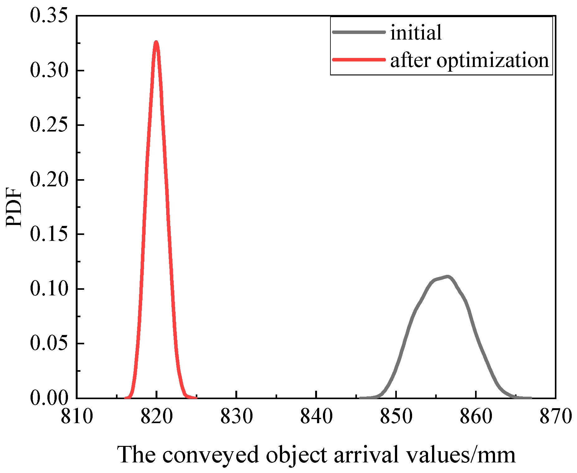
The robust optimization design method can effectively improve the transmission accuracy of the chain transmission mechanism. Compared to the initial design, the variance of the transported object is reduced by 63.14%.

(4)

The optimized results prove the effectiveness of the proposed method in improving the consistency of the conveyed object positioning. This method and its results provide theoretical guidance for the design of chain transmission mechanisms.

This article also has certain limitations. Due to the complexity of the chain transmission mechanism model, certain simplifications and assumptions were made during the dynamic modeling process, which had a slight effect on the accuracy of the dynamic model. In future work, the method proposed in this paper can be extended to the design process of other chain transmission mechanisms to improve motion robustness. Furthermore, to enhance the service reliability of chain transmission mechanisms, further research can focus on time-varying robust optimization design based on reliability. This will better promote the application and development of chain transmission systems in complex environments, providing stronger theoretical support and technical assurance for the engineering design of chain transmission mechanisms.

References

1. Li, Y.; Qian, L.; Chen, G.; Huang, W. Multiple clearance robustness optimization of a chain ramming machine based on a data-driven model. Nonlinear Dyn. 2023, 111, 13807–13828. [Google Scholar] [CrossRef]
2. Zhuang, M.; Li, G.; Ding, K.; Xu, G. Optimized design of mechanical chain drive based on a wireless sensor network data algorithm. J. Sens. 2021, 2021, 2901624. [Google Scholar] [CrossRef]
3. Chai, M.; Yuan, Y.; Zhao, W. An improved particle swarm optimization algorithm for dynamic analysis of chain drive based on multidisciplinary design optimization. Adv. Mech. Eng. 2019, 11, 1687814019829611. [Google Scholar] [CrossRef]
4. Jiang, S.B.; Huang, S.; Zeng, Q.L.; Wang, C.L.; Gao, K.D.; Zhang, Y.Q. Dynamic properties of chain drive system considering multiple impact factors. Int. J. Simul. Model 2022, 21, 284–295. [Google Scholar] [CrossRef]
5. Hong, L.; Li, X.J. Structural optimization of a chain transmission with constraints. Appl. Mech. Mater. 2014, 687, 523–526. [Google Scholar] [CrossRef]
6. Da, L.; Ying, L.; Zheng, G.; Sun, M.; Liang, Z. Design of mechanical chain drive based on particle swarm optimization. In Proceedings of the 2022 International Conference on Intelligent Transportation, Big Data & Smart City (ICITBS), Hengyang, China, 26–27 March 2022; IEEE: New York, NY, USA, 2022; pp. 97–101. [Google Scholar]
7. Cheng, Y.; Guo, H.; Fu, Z.; Wan, N.; Li, L.; Wang, Y. Design and analysis of the Gemini chain system in dual clutch transmission of automobile. Chin. J. Mech. Eng. 2015, 28, 38–45. [Google Scholar] [CrossRef]
8. Wang, Y.; Du, J.; Yang, T.; Zhou, J.; Wang, B.; Shi, Y.; Bai, J. Robust Optimization Design of a Blended Wing-Body Drone Considering Influence of Propulsion System. Aerosp. Sci. Technol. 2024, 156, 109751. [Google Scholar] [CrossRef]
9. Zhang, W.; Qiang, W.; Fanzhi, Z.; Chao, Y. A novel robust aerodynamic optimization technique coupled with adjoint solvers and polynomial chaos expansion. Chin. J. Aeronaut. 2022, 35, 35–55. [Google Scholar] [CrossRef]
10. Najlawi, B.; Nejlaoui, M.; Affi, Z.; Romdhane, L. Multi-objective robust design optimization of a sewing mechanism under uncertainties. J. Intell. Manuf. 2019, 30, 783–794. [Google Scholar] [CrossRef]
11. Zhang, Y.; Chen, L.; Chen, G.; Liu, T. Data-Driven Modeling and Robust Optimization of the Ammunition Ramming Mechanism Based on Artificial Neural Network. In Proceedings of the International Conference on Mechanical System Dynamics, Beijing, China, 1–5 September 2023; Springer Nature: Singapore, 2023; pp. 691–705. [Google Scholar]
12. Gao, H.; Sun, G.; Liu, Z.; Sun, C.; Li, N.; Ding, L.; Yu, H.; Deng, Z. Tension distribution algorithm based on graphics with high computational efficiency and robust optimization for two-redundant cable-driven parallel robots. Mech. Mach. Theory 2022, 172, 104739. [Google Scholar] [CrossRef]
13. Guo, F.; Sun, Z.; Zhang, S.; Cao, R.; Li, H. Optimal design and reliability analysis of a compliant stroke amplification mechanism. Mech. Mach. Theory 2022, 171, 104748. [Google Scholar] [CrossRef]
14. Wu, W.; Rao, S.S. Uncertainty analysis and allocation of joint tolerances in robot manipulators based on interval analysis. Reliab. Eng. Syst. Saf. 2007, 92, 54–64. [Google Scholar] [CrossRef]
15. Du, X.; Venigella, P.K.; Liu, D. Robust mechanism synthesis with random and interval variables. Mech. Mach. Theory 2009, 44, 1321–1337. [Google Scholar] [CrossRef]
16. Krüger, J.C.; Kranz, M.; Schmidt, T.; Seifried, R.; Kriegesmann, B. An efficient and non-intrusive approach for robust design optimization with the first-order second-moment method. Comput. Methods Appl. Mech. Eng. 2023, 414, 116136. [Google Scholar] [CrossRef]
17. Meng, Z.; Wu, Y.; Wang, X.; Ren, S.; Yu, B. Robust topology optimization methodology for continuum structures under probabilistic and fuzzy uncertainties. Int. J. Numer. Methods Eng. 2021, 122, 2095–2111. [Google Scholar] [CrossRef]
18. Kriegesmann, B.; Lüdeker, J.K. Robust compliance topology optimization using the first-order second-moment method. Struct. Multidiscip. Optim. 2019, 60, 269–286. [Google Scholar] [CrossRef]
19. Cheng, J.; Lu, W.; Liu, Z.; Wu, D.; Gao, W.; Tan, J. Robust optimization of engineering structures involving hybrid probabilistic and interval uncertainties. Struct. Multidiscip. Optim. 2021, 63, 1327–1349. [Google Scholar] [CrossRef]
20. Lee, S.H.; Chen, W.; Kwak, B.M. Robust design with arbitrary distributions using Gauss-type quadrature formula. Struct. Multidiscip. Optim. 2009, 39, 227–243. [Google Scholar] [CrossRef]
21. Chatterjee, T.; Chowdhury, R.; Ramu, P. Decoupling uncertainty quantification from robust design optimization. Struct. Multidiscip. Optim. 2019, 59, 1969–1990. [Google Scholar] [CrossRef]
22. Lee, D.; Rahman, S. Robust design optimization under dependent random variables by a generalized polynomial chaos expansion. Struct. Multidiscip. Optim. 2021, 63, 2425–2457. [Google Scholar] [CrossRef]
23. Zafar, T.; Zhang, Y.; Wang, Z. An efficient Kriging based method for time-dependent reliability based robust design optimization via evolutionary algorithm. Comput. Methods Appl. Mech. Eng. 2020, 372, 113386. [Google Scholar] [CrossRef]
24. Jiang, Z.; Wu, J.; Huang, F.; Lv, Y.; Wan, L. A novel adaptive Kriging method: Time-dependent reliability-based robust design optimization and case study. Comput. Ind. Eng. 2021, 162, 107692. [Google Scholar] [CrossRef]
25. Cheng, J.; Wang, R.; Liu, Z.; Tan, J. Robust equilibrium optimization of structural dynamic characteristics considering different working conditions. Int. J. Mech. Sci. 2021, 210, 106741. [Google Scholar] [CrossRef]
26. Pereira, C.; Ambrósio, J.; Ramalho, A. Dynamics of chain drives using a generalized revolute clearance joint formulation. Mech. Mach. Theory 2015, 92, 64–85. [Google Scholar] [CrossRef]
27. Pedersen, S.L. Model of contact between rollers and sprockets in chain-drive systems. Arch. Appl. Mech. 2005, 74, 489–508. [Google Scholar] [CrossRef]
28. Ma, J.; Bai, M.; Wang, J.; Dong, S.; Jie, H.; Hu, B.; Yin, L. A novel variable restitution coefficient model for sphere–substrate elastoplastic contact/impact process. Mech. Mach. Theory 2024, 202, 105773. [Google Scholar] [CrossRef]
29. Ma, J.; Wang, J.; Peng, J.; Yin, L.; Dong, S.; Tang, J. Data-driven modeling for complex contacting phenomena via improved neural networks considering link switches. Mech. Mach. Theory 2024, 191, 105521. [Google Scholar] [CrossRef]
30. Movahedi-Lankarani, H. Canonical Equations of Motion and Estimation of Parameters in the Analysis of Impact Problems. Ph.D. Thesis, University of Arizona, Tucson, AZ, USA, 1988. [Google Scholar]
31. Liu, T.; Niu, Y.; Chen, G. A general methodology for simulation model validation and model updating of the coordination mechanism with uncertainty. J. Mech. Sci. Technol. 2023, 37, 6271–6286. [Google Scholar] [CrossRef]
32. Bae, D.S.; Han, J.M.; Choi, J.H. An implementation method for constrained flexible multibody dynamics using a virtual body and joint. Multibody Syst. Dyn. 2000, 4, 297–315. [Google Scholar] [CrossRef]
33. Tong, M.N.; Zhao, Y.G.; Zhao, Z. Simulating strongly non-Gaussian and non-stationary processes using Karhunen–Loève expansion and L-moments-based Hermite polynomial model. Mech. Syst. Signal Process. 2021, 160, 107953. [Google Scholar] [CrossRef]
34. Blatman, G.; Sudret, B. Adaptive sparse polynomial chaos expansions based on Least Angle Regression. J. Comput. Phys. 2011, 230, 2345–2367. [Google Scholar] [CrossRef]
35. Chen, G.S. The Study on the Dynamic of the Projectile-Barrel Coupled System and the Corresponding Key Parameters. Ph.D. Thesis, University of Science and Technology, Nanjing, China, 2016. [Google Scholar]
36. Efron, B.; Hastie, T.; Johnstone, I.; Tibshirani, R. Least Angle Regression. Annels Stat. 2004, 32, 407–499. [Google Scholar] [CrossRef]
Figure 1. Schematic diagram of chain transmission mechanism (in the plane).
Machines 13 00166 g001
Figure 2. Topological relationship of the chain transmission mechanism.
Machines 13 00166 g002
Figure 3. Schematic diagram of chain system.
Machines 13 00166 g003
Figure 4. Geometrical diagram of sprocket tooth groove.
Machines 13 00166 g004
Figure 5. Contact relationship between roller and positioning curve of sprocket tooth groove.
Machines 13 00166 g005
Figure 6. Contact relationship between roller and top curve of sprocket tooth groove.
Machines 13 00166 g006
Figure 7. Contact relationship between adjacent chain links.
Machines 13 00166 g007
Figure 8. The test schematic diagram of the propellant transport process.
Machines 13 00166 g008
Figure 9. The torque curve for the sprocket.
Machines 13 00166 g009
Figure 10. The comparison of simulation displacement and experiment displacement for the modular charge.
Machines 13 00166 g010
Figure 11. The torque design curve for the sprocket.
Machines 13 00166 g011
Figure 12. The test result of the propellant transport mechanism’s PCE model.
Machines 13 00166 g012
Figure 13. The Pareto optimal solution set of the propellant transport process.
Machines 13 00166 g013
Figure 14. PDF of the modular charge displacement before and after optimization.
Machines 13 00166 g014